Abstract
Urban spatial structures (USS) play an essential role in urbanization. Understanding the impact of USS patterns on their socioeconomic benefits is crucial to evaluating urban structure quality. Previous studies have, primarily, relied on statistical data and have significant temporal consistency and spatial accuracy limitations. Moreover, previous evaluation methods mainly determined the weight of indicators based on subjective assessments, such as the Delphi method, without integrating the actual socioeconomic benefits of complex urban systems. By measuring the two-dimensional (2D) urban functional landscape patterns and three-dimensional (3D) building forms of the city and considering the level of urban socioeconomic vitality as revealed by nighttime light intensity (NTLI), this study explores the influence of urban spatial structure on socioeconomic vitality. It provides a new perspective for evaluating the USS level. Furthermore, a comprehensive index, namely the Spatial Structure Socioeconomic Benefit Index (SSSBI), was constructed to quantify the socioeconomic benefits of USS. The results showed that (1) the impact of spatial structure on NTLI differs significantly with the distribution of urban functional landscape patterns and building forms. (2) The combined effect of any two spatial structure factors on NTLI was higher than the effect of each factor separately, indicating that multiple dimensions can improve urban spatial construction. (3) This study quantitatively extracts the characteristics of USS from multiple scales, which helps to find the optimal evaluation scale and build a scientific and objective evaluation model. The results showed that the USS assessment based on the SSSBI index is practical. This study could provide a reference for the government’s urban planning and land-use decisions.
1. Introduction
In the 21st century, the level of urbanization has been unprecedentedly developed, but at the same time, some urban problems in economic, social, resource, and environmental aspects have emerged [1,2]. Currently, the international community has put forward higher demands for urban development, and scholars have paid increasing attention to research on urban development [3,4]. Therefore, it has become increasingly important to measure the state of urban development scientifically.
The physical environment and socioeconomic space development are crucial to the urban development process [5,6]. The former is mainly manifested in the expansion of urban boundaries and the change of internal spatial structure [7]. The latter is considered to be socioeconomic changes generated by the activities of urban residents, such as economic growth, lifestyle changes, etc., [8,9]. The physical environment and socioeconomic development of cities are mainly driven by population clustering, and the results of their development are also reflected in the lives of urban residents; these two aspects have the same roots and are inseparable [10,11]. Therefore, in urban development research, focusing on the coupling relationship between the two is essential for a comprehensive evaluation of the state of urban development.
Over the past 20 years, remote sensing technology has developed rapidly, and remote sensing data have been widely used in urban spatial research. On the one hand, Landsat satellites, Sentinel series satellites, and Gaofen series satellites have been launched, and some medium- and high-resolution remote sensing data are shared for free, which has made the study of urban spatial structure (USS) based on remote sensing data a hot topic of current research [12]. However, with the availability of night light remote sensing data, remote sensing technology can be used to detect urban socioeconomic development [13]. Since remote sensing data carry spatial information and have better spatial expression ability than statistical data, luminous remote sensing data have become the link between the physical and socioeconomic environment levels in urban development research and play an essential role in urban socioeconomic spatial analysis [14,15,16,17,18,19]. In addition, an increasing number of researchers have recognized the application of the Internet and communication technologies to geography [20]. Compared with traditional data, new data, such as Point of Interest (POI) and map navigation, usually have the characteristics of a large amount of data, fast transmission, rich information, and low cost, which can be used to analyze the spatiotemporal patterns of human activities and provide new ideas for revealing the spatial structure characteristics and socioeconomic features of urban areas [21,22]. Advancements in high-resolution remote sensing and the abundance of data sources have provided great convenience for researchers to evaluate the quality of urban space at a finer scale and from a more dimensional perspective [23,24].
In this context, many researchers are working to explore the relationship between USS patterns and the socioeconomic environment. Many studies have considered land-use patterns as important assessment indicators for the development of USS [25]. They have produced various land-use products based on traditional classification methods, including the index, supervised, unsupervised, and emerging classification methods (i.e., machine learning and deep learning) [26,27,28]. However, these studies mainly classified land cover directly based on the physical attributes of features, and there are few studies related to the identification and distribution of urban functional scenes. Urban functional areas are geographical spaces that show the functions of urban areas and contain a series of social and economic attributes of land use [29]. However, thus far, few attempts have been made to study the impact of the functional structure of land use on urban socioeconomics. Therefore, analyzing the functional pattern of urban land use can help evaluate USS and its socioeconomic benefits more comprehensively.
Urban buildings are also essential to the USS and are important carriers of human social and economic activities [30]. The studies of edge extraction of urban buildings and building height extraction based on high-resolution remote sensing images have also become research hotspots [31,32,33,34,35]. With accelerated urbanization, the expansion pattern of cities has shifted from horizontal to vertical directions, while higher urban building heights accommodate more people and their socioeconomic activities [36,37]. Although some studies have incorporated three-dimensional (3D) information into the analysis of urban spatial structures, research on the driving effect of 3D building form on socioeconomic vitality is insufficient [38,39,40]. Therefore, it is crucial to explore the characteristics of 3D spatial structures and their impact mechanism on urban socioeconomic development.
In summary, this study first used high-resolution remote sensing images, POI data, and 3D building data to express urban spatial structure patterns, including functional landscape patterns and building forms. It also used nighttime light remote sensing data to express the intensity of urban socioeconomic activities. Then, feature extraction was performed at ten scales to achieve a multi-scale, multi-dimensional spatial expression of the city’s spatial structure and socioeconomic vitality. Finally, correlation, geographic probe, and random forest regression analyses were used to further explore the influence mechanisms of urban spatial structure and socioeconomic vitality. To this end, this study explores and answers the following questions: (1) How large is the spatial scale of the influence of urban spatial structure on urban socioeconomic activities? (2) What is the intensity of the influence of different urban spatial structure features on urban socioeconomic activities? (3) How can a more objective and practical evaluation index of urban spatial structure quality be developed? (4) What are the spatial characteristics of the spatial structure distribution in the study area?
2. Materials and Methods
2.1. Study Area
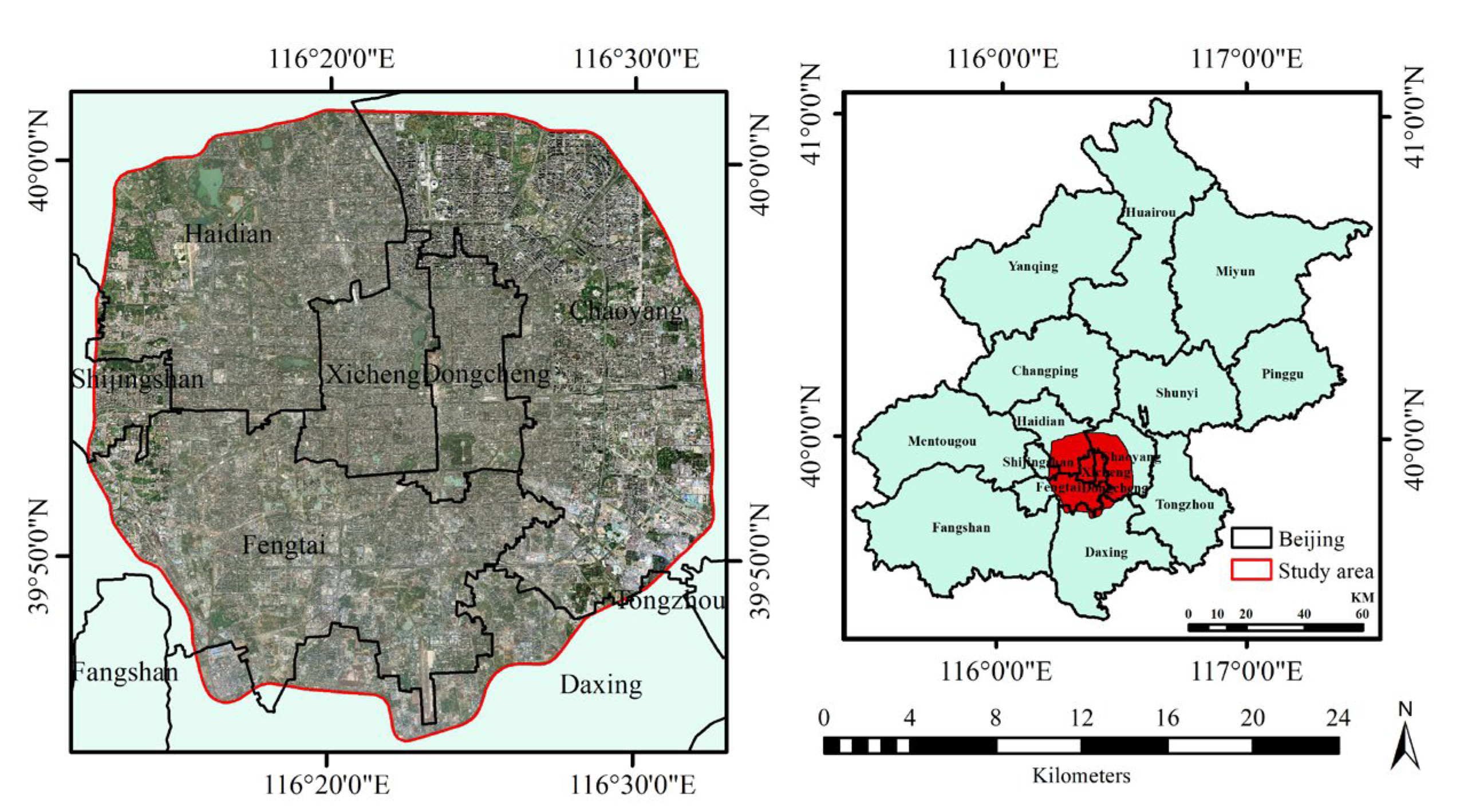
Beijing (39.9042°N, 116.4074°E) is the capital, political, economic, international communication, science, and technology innovation center of China. As of 2021, Beijing has a total area of 16,410.54 km2 and 16 districts, with a resident population of 21.893 million and an urbanization level of 86.2%, making it one of the seven megacities in China. We focus on the area within Beijing’s Fifth Ring Road (Figure 1), which is the core area, accounting for only approximately 4% of the city’s total area but is inhabited by nearly half of the city’s population.
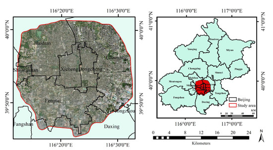
Figure 1.
The study area, within the Fifth Ring Road of Beijing, includes the city’s urban area.
In the context of increasingly prominent urban diseases in China, in recent years, the Beijing government has made great efforts to improve the quality of the urban environment using urban physical examination and urban renewal and has achieved remarkable results. Nevertheless, since urban diseases in Beijing have accumulated for many years and are relatively difficult to solve, there is a great need to launch an accurate measure, rational analysis, and evaluation of the spatial structure of Beijing to provide ideas for the management of urban diseases in Beijing.
2.2. Used Data
Five geographic data points were considered to analyze the spatial structure pattern of the general study area: satellite image data, POI data, OSM data, building data, and nighttime light data. The first three identify the functional characteristics of urban land use, the fourth is used to explore the urban 3D building morphology, and the last extracts the nighttime light intensity.
- Satellite images. We obtained a satellite image from the ESRI image product, which was generated by splicing images from different sensors. It was produced in 2021 with three bands (red, green, and blue) with a spatial resolution of 4.11 m. The original image has been corrected and stitched, and projection conversion and cropping are required to provide accurate image feature information before use.
- POI data. We collected 359,659 POI in 2021 from Amap (https://www.amap.com/ (accessed on 22 November 2021)), a leading digital mapping, navigation, and location service company in China, whose data are updated frequently so that accurate and reliable information on the location and function of POIs is available. In this paper, Arcgis10.7 software is first used to preprocess POI data, including vector transformation, coordinate transformation, removal of duplication, and missing information points. Then, these POIs were reclassified into 11 categories: government institutions, medical service facilities, sports facilities, educational and cultural service facilities, commercial service facilities, business service facilities, business residences, residential areas, transportation facilities, industrial facilities, and scenic and recreational service facilities. POI is closely related to the activities of residents and the configuration of urban facilities and thus contributes to the analysis of the urban spatial structure.
- Road network data. OpenStreetMap (https://www.openstreetmap.org/ (accessed on 8 September 2021)) is a free, open-source, editable nonprofit mapping service data. This study selected primary, secondary, tertiary, trunk, and residential road network line data from the 2021 OSM data. Arcgis10.7 software was used for clipping, topology checking, line turning polygon, and buffer processing, and then constructed the urban block unit data based on road network data to assist the functional area classification labeling samples.
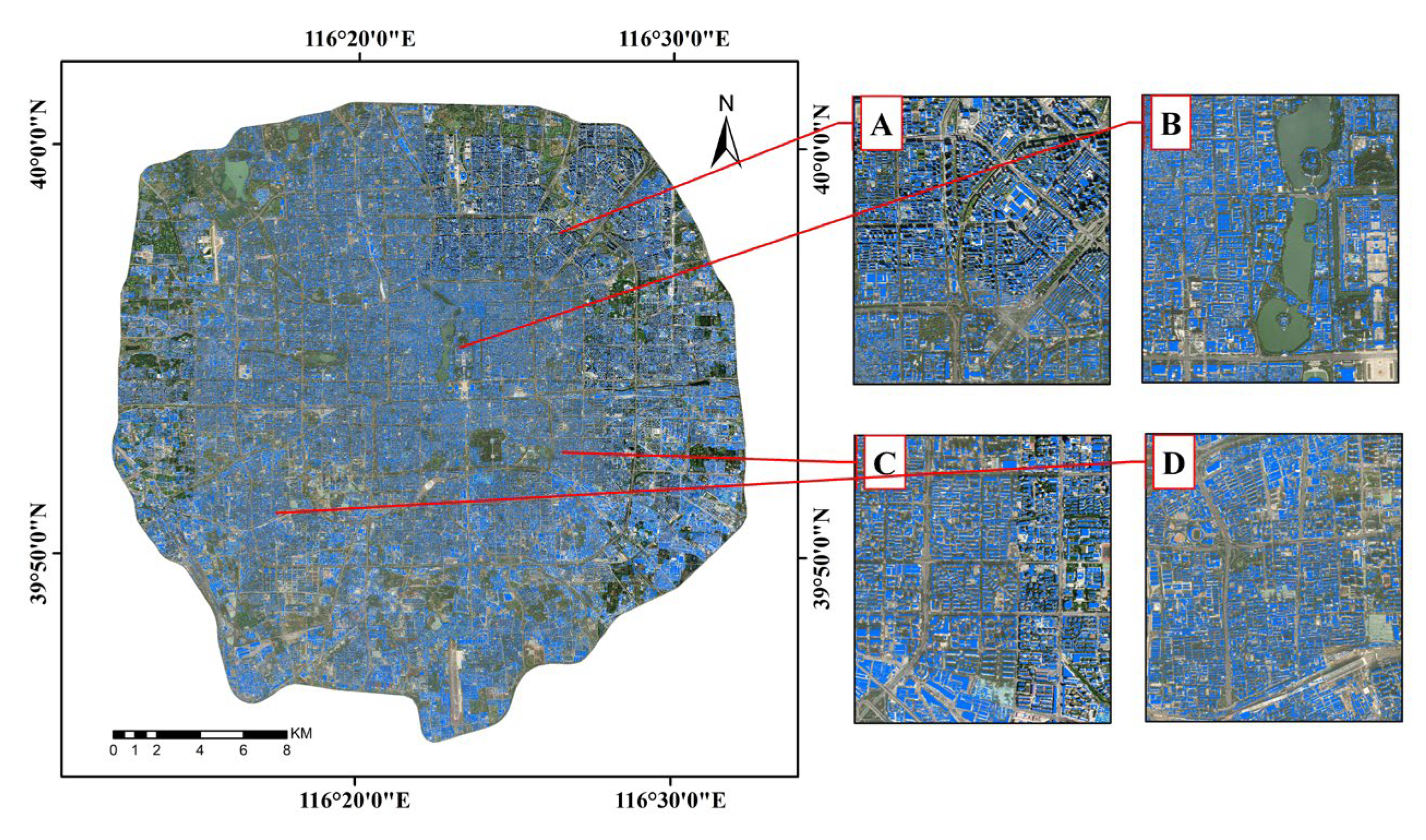
- Buildings data. In May 2021, we collected information on 402,927 buildings from AMap, which are presented as vector polygons. This can provide the bottom profile and height of buildings for urban studies. As shown in Figure 2, overlaying the buildings with satellite images shows that almost all the buildings in the study area are included.
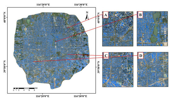 Figure 2. Building data overlaid with satellite images. ((A–D) are the four sample regions for display.)
 - Nighttime light data. Nighttime light intensity (NTLI) has been widely used to estimate socioeconomic metrics, such as gross domestic product (GDP), population, total freight, housing vacancy rate, poverty, and CO2 emissions [41,42,43,44,45]. Numerous investigations have confirmed the ability of the NTLI to reflect human socioeconomic activities, which can be a better alternative for urban socioeconomic activity intensity [46,47,48]. In this study, we used nighttime light remote sensing data from the Luojia1-01 star from the high-resolution Earth observation system (EOS), technology, and application (https://www.hbeos.org.cn/ (accessed on 6 November 2021)). The image was acquired in November 2018 with a spatial resolution of 130 m, which can be used to characterize socioeconomic activities at a fine scale within urban areas. To obtain valid light values, ENVI 5.3 software was used for pre-processing, including coordinate system conversion, radiance conversion, data clipping, partition statistics, and data connection.
2.3. Methods
This study investigated the influence of urban spatial structure on socioeconomic development status. First, to explore the spatial distribution and landscape pattern characteristics of urban land-use functions, a convolutional deep learning method is used to propose a classification method for land-use functional areas. Second, we need to extract features from the data to explore the relationship between urban functional landscape patterns, building forms, and socioeconomic vitality. This section proposed a multi-scale feature statistics method to extract the urban spatial structure and economic features from ten scales. Third, we applied various analytical methods, such as random forest regression analysis and geographic detector analysis, to analyze the driving effects of urban spatial structures on socioeconomic vitality. Finally, the analytic hierarchy process (AHP) method was used to comprehensively evaluate the quality of the urban spatial structure and construct the spatial structure socioeconomic benefit index.
Figure 3 shows the flow chart of this study, and the key methods used are described in detail in this section.
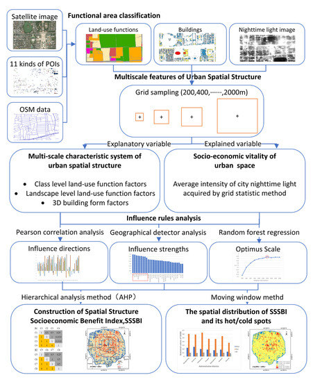
Figure 3.
Flowchart of this study.
2.3.1. Land-Use Function Classification Method
Land-use functional areas are highly heterogeneous and difficult to identify using traditional classification methods. Multi-source data fusion classification can identify more data features and achieve better results than the corresponding single-source data. Therefore, this study used remote sensing images and POI data, combined with deep learning methods, to classify urban functional areas.
Figure 4 shows the segmentation framework for recognizing land use functions. First, we converted the 11 POI datasets into kernel density images with a radius of 700 m [49]. Then, the POI density maps were separately normalized to [0, 1] and superimposed into an overall map as input. Next, the image features were encoded through the Atrous Spatial Pyramid Pooling (ASPP) module [50]. Four parallel convolutions with different expansion rates were used to process the feature maps. Small-scale input responses controlled the semantics and large-scale input responses controlled the details, the features are resampled at different scales, allowing accurate and efficient classification of regions at arbitrary scales. Finally, the generated feature maps were further processed by convolution and upsampling operations to predict the classification results of land-use functions for each pixel.

Figure 4.
Segmentation framework for recognizing land-use functions.
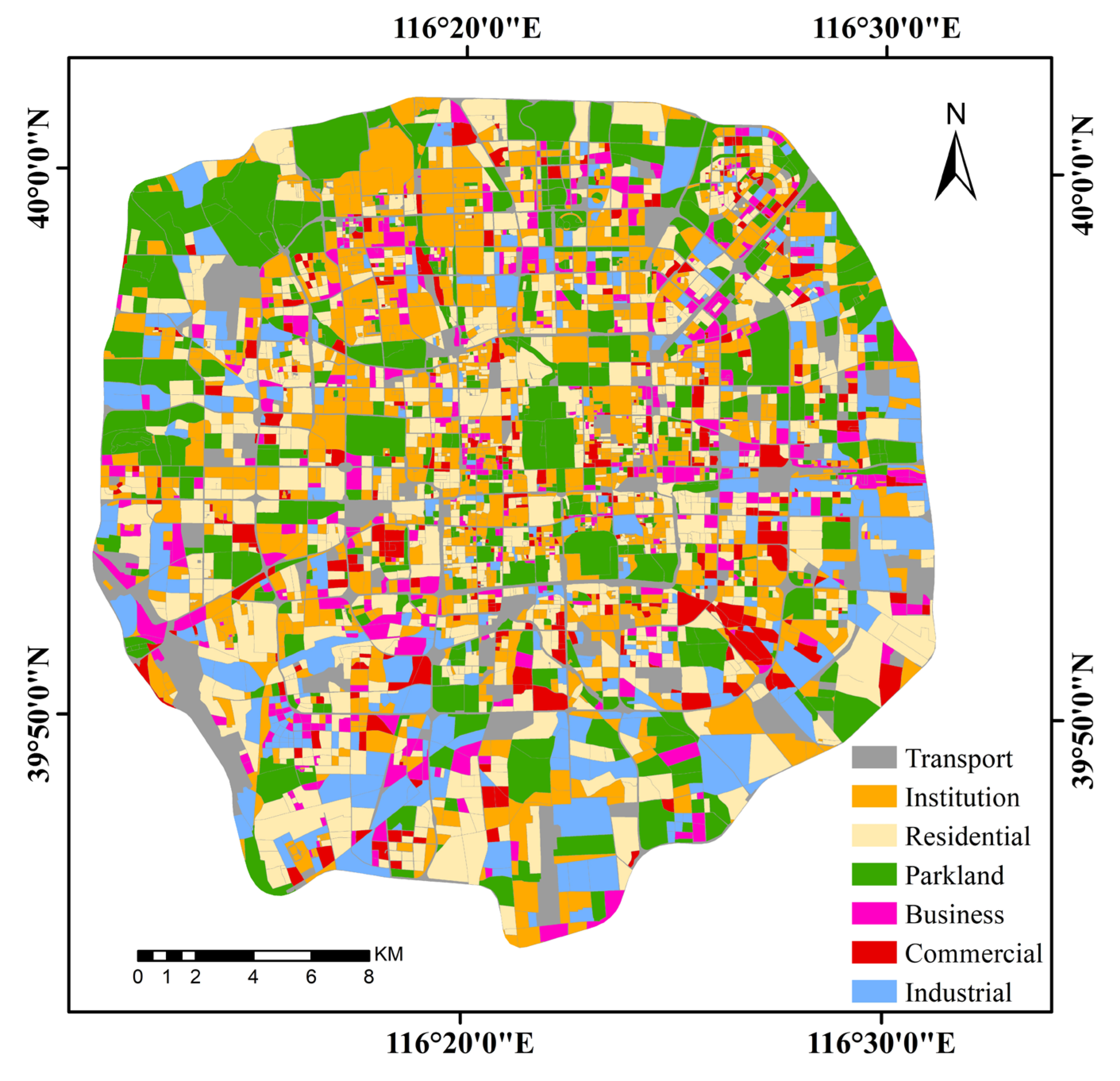
Supervised samples are required to train the model. In this paper, OSM vector data are firstly processed by data filtering, topology checking, data cropping, and buffering to construct the basic units of urban functional areas based on parcel polygons. Then, referring to satellite images and Baidu maps, four thousand three hundred eighty-seven (4387) functional area samples were assigned to categories. Finally, the vector data is transformed into raster image and input into neural networks, which can provide boundary constraints and sample labels for classification of functional areas, and help to complete model training and category prediction. The overall classification accuracy is 86.72%. Figure 5 shows the distribution of functional areas, and Table 1 shows the confusion metrics of classification result accuracy evaluation.

Figure 5.
The generated land-use function map.

Table 1.
Sample numbers and accuracies of functional zone classification results.
As shown in Table 1, most categories were accurately identified with an accuracy rate greater than 80%. Still, the accuracy rate of commercial areas was relatively poor because of their complex structure and different representations. The overall accuracy of the classification was 86.43%, indicating that the land-use functional map was accurate enough to be used for USS analysis.
The land-use function map shows the regional divisions of urban functions. To further study the spatial connection and distribution characteristics among various landscapes, this study used Fragstats 4.2 software to calculate the landscape pattern index of functional areas based on the land-use function classification map [51]. The calculation of the landscape pattern index was divided into class-level and landscape-level metrics, which described the single category and overall spatial layout of the landscape, respectively. Class-level and landscape-level metrics provided complementary information to refine the quantitative description of landscape pattern characteristics.
2.3.2. Multi-Scale Feature Statistical Method
As shown in Table 2, fourteen indicators were selected to characterize the city’s spatial structure. Among them, eight widely used landscape indicators were selected to measure the distribution of urban functional patterns, except for the Shannon Diversity Index (SHDI), which was analyzed at the landscape level, and all other indicators were analyzed at both the landscape and class levels. In addition, considering the accuracy and practicality, six building morphology indicators, including two two-dimensional (2D) and four three-dimensional (3D) indicators, were selected to analyze the 3D form of urban buildings, quantitatively. Finally, the average NTLI measured a city’s socioeconomic activity level.

Table 2.
Introduction of statistical analysis metrics.
In Table 2, Hi, Vi, and Fi are the height (m), volume (m3), and building footprint (m2) of the i-th building, respectively; n is the number of buildings, and A is the area of the analysis area (m2). c = 3.0 m is a constant, Hmax is the maximum height of buildings in the area (m), and Hmin is the minimum height of buildings in the area (m). Li is the nighttime light intensity.
To quantitatively measure urban spatial structure features, this study proposed a multi-scale statistical method to express these features. Grid sizes of 200 m × 200 m, 400 m × 400 m, 600 m × 600 m, 800 m × 800 m, 1000 m × 1000 m, 1200 m × 1200 m, 1400 m × 1400 m, 1600 m × 1600 m, 1800 m × 1800 m, 2000 m × 2000 m were used for multi-scale sampling to comprehensively analyze the scale, direction, and intensity of the effect of urban spatial structure on NTLI.
2.3.3. Geographical Detector Method
A geographical detector is a statistical method for detecting spatial differentiation and revealing its influences [52]. It can detect the extent to which factors explain a phenomenon and analyze its causes [53]. Geographical detector models have two main advantages. First, the model can detect numerical and qualitative data [54]. Another advantage is the ability to calculate the explanatory power of the interaction between the two factors.
In this study, factor detection was used to assess the extent to which factor X (USS indicators) explain the spatial variance of the dependent variable Y (NTLI). Here, the q statistic can be used to measure.
Here, q is the explanatory power of the requested driver, k (k = 1, 2, 3, …, m) is the number of strata of factor X or independent variable Y; Nk and N are the number of units in strata k and the whole region, respectively; δk2 and δ2 are the variances of Y for layer h and the whole region, respectively. The value of q indicates that X explains q% of Y. A larger value of q indicates that the independent variable X explains more of attribute Y and vice versa. At the extreme, q = 1 indicates that factor X completely controls the spatial distribution of Y, whereas q = 0 indicates that factor X has no relationship with Y.
In addition, interaction detection can be used to identify interactions between different factors (XS); for example, to evaluate whether factors X1 and X2 together increase or decrease the explanatory ability of the dependent variable Y. Central to this is the comparison of q-values driven by two separate factors and by the interaction of the two.
2.3.4. Random Forest Regression (RFR) Method
This study investigated the impact of USS on socioeconomic vitality and modeled the correlation between the USS features and the mean NTLI, which can be achieved by establishing regression models. The random forest regression (RFR) model is an integrated learning algorithm based on decision trees. Compared to traditional multiple regression analysis, RFR can effectively handle high-dimensional data and has better regression fitting with fewer parameters to adjust in the model.
Regression in random forest is performed by combining several regression trees fitted to the training samples and predicted as regression results. First, from each regression tree, a series of samples were randomly selected, and then trained using the bagging technique, whereas other non-selected out-of-bag samples (OOB) were used to evaluate the regression error [55]. If putback sampling is selected during tree-building, approximately 1/3 of the records are not sampled, which naturally form a control dataset that can be used for model validation. Therefore, the random forest does not need to set aside an additional portion of data for cross-validation, its algorithm is similar to cross-validation [56].
In this study, the USS features were considered independent variables, NTLI was the dependent variable for building an RFR model. Regression coefficients (R2) and OOB errors determine the model fit’s accuracy. Accordingly, an optimal analysis scale with the highest fitting accuracy was obtained.
2.3.5. Analytic Hierarchy Process (AHP) Method
Hierarchical analysis is a multi-criteria decision-making method that combines qualitative and quantitative analysis [57]. The basic idea is to construct a simple hierarchical structural model after an in-depth analysis of a complex decision’s core requirements, influencing factors, and intrinsic relationships. In this study, AHP was used to convert the results of the geographical detector into the weights of the evaluation indicators.
Specifically, the hierarchical analysis method starts by decomposing the complex problem into individual indicators, and then grouping these indicators into the target, criterion, and solution levels [58]. A stratified discussion is then conducted to compare the importance of the metrics within and between levels, and using Saaty’s idea of the 1–9 scale method to obtain a judgment matrix A [59]. Finally, based on matrix A, the weight values of each indicator were calculated. In addition, the consistency of judgment matrix A must be tested against its maximum characteristic roots.
where λmax is the maximum eigenvalue of the comparison matrix and n is the order of the matrix. CI is the consistency indicator of the calculated matrix; the larger the CI, the greater the deviation from the consistency of the judgment matrix A. RI is the average random consistency indicator, which corresponds to n. When n is 1–10, RI is 0, 0.58, 0.90, 1.12, 1.24, 1.32, 1.41, 1.45, and 1.49, respectively. If CR < 0.1, judgment matrix A is considered to have acceptable consistency; otherwise, the values of each element in A need to be reset.
Thus, the weights of all the indicators in the stratification were obtained. The analysis results of the geographic detector were used to quantitatively evaluate the stratification and weights of the model to better balance the subjectivity and objectivity of the weight setting.
3. Results
3.1. Optimal Scale for USS Analysis
As mentioned in Section 2.3.2, this study measured the coupling between USS characteristics and NTLI at multiple scales. Therefore, at which scale do USS characteristics more accurately reflect the level of socioeconomic activity? The relationship between urban spatial structure patterns and NTLI was modeled by random forest regression in Section 2.3.4 so that the regression errors are useful for assessing multiple scales.
In total, we created a sampling grid at 10 scale levels to select the optimal scale for analyzing the socioeconomic benefits of USS. The features of the spatial structure patterns listed in Table 2 were measured at each of the 10 scales and integrated with NTLI for training the random forest regression models and, ultimately, to calculate OOB errors and R2. As shown in Figure 6, R2 gradually increased at 200 m ≤ scale ≤ 1400 m, reaching a maximum value of 93.9% at the 1400 m scale, while the OOB error decreased to the lowest value. This indicates that the regression results become increasingly accurate in this scale range, suggesting that within 1400 m, the change in the statistical scale significantly impacts the evaluation of USS’s socioeconomic benefits. Subsequently, after the 1400 m scale, the R2 value remains relatively stable, and the OOB error also fluctuated around the lowest value, indicating that the change in the statistical scale does not affect the socioeconomic benefits of USS when the statistical scale exceeds 1400 m.
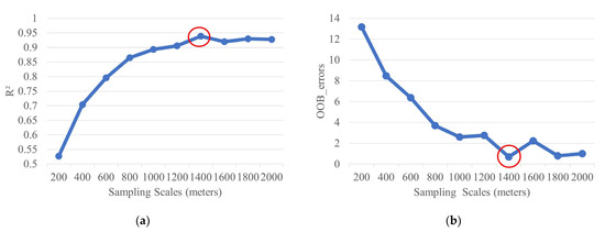
Figure 6.
(a) The dynamic changes of the regression coefficients (R2) with increasing the scale; (b) The dynamic changes of the out-of-bag (OOB) error with increasing the scale. Both OOB error and R2 are calculated by the random forest method.
Accordingly, the influence of USS features on NTLI was significant, and 1400 m, which has the lowest fitting error and highest regression coefficient, was the best scale for analyzing the impact of the USS model on NTLI. Therefore, in the next section, we continue to analyze the correlation and driving strength of each USS factor on NTLI at the 1400 m scale.
3.2. Analysis of the Relationship between USS Features and NTLI
3.2.1. Correlation of Diverse USS Features on NTLI
The Pearson correlation coefficient and the Spearman correlation coefficient are two commonly used correlation analysis methods, which can detect both the correlation degree and direction. between the dependent and independent variables. In this study, we tested the normality of the data and found that it did not conform to the standard normal distribution. Therefore, the Spearman correlation analysis is more suitable for this study.
Table 3 shows that more than 85% of the indicators were significantly correlated with the NTLI, and the number of positively correlated indicators and the correlation coefficients are much larger than those of the negatively correlated indicators. All indicators at the building-form level were positively correlated with NTLI, and 3D indicators with height information had higher correlation coefficients than 2D indicators. AM had the strongest correlation with NTLI, with a correlation coefficient of 0.703. Among the landscape pattern indicators, those under commercial, business, residential, and institutional categories were positively correlated with NTLI. Among them, the highest correlation coefficient was found for indicators under the category level of the business area.

Table 3.
Correlation coefficient between USS features and NTLI. Red represents positive correlation; green represents negative correlation; the darker the color, the stronger the correlation.
As can be seen from Table 3, SPLIT at the landscape level showed a positive correlation with NTLI, with a correlation coefficient of 0.702, which was the highest value of all landscape pattern index levels. However, at the class level, the SPLIT of transport had a negative correlation with NTLI, indicating that road connectivity plays an important role in the economic and social development of the city.
At the landscape level, MESH and LPI were negatively correlated with NTLI; at the class level, the MESH and LPI of parkland and industrial areas were also negatively correlated with NTLI. This indicates that as the area of land patches increases, the landscape type with a larger area becomes the dominant factor of local socioeconomic activities. Industrial areas and parklands have low land utilization rates and few traces of urbanization, which is not conducive to the large concentration of population and socioeconomic activities. Therefore, large concentrations of industry and green areas tend not to promote NTLI.
The correlation coefficients show that constructing high-rise buildings, increasing the functional categories of the city, and concentrating on commercial and business districts while paying attention to the rational allocation of green spaces and factories, are conducive to enhancing NTLI and the dynamic socioeconomic development of the city.
3.2.2. Driving Effects of Diverse USS Features on NTLI
Sixty-three drivers were quantified using a factor detector. These indicators contained three categories, class, landscape, and built form, with 49, 8, and 6 indicators in each category, respectively. Table 2 in Section 2.3.2 shows these indicators. All indicators were drivers of NTLI (p < 0.01). There were different explanatory rates for NTLI spatially stratified heterogeneity. Among the land-use functional pattern indicators, the interpretation rates were as follows: landscape-level indicators > class-level indicators. Among the building form-level indicators, the explanatory rate was ordered as follows: 3D building form indicators > 2D building form indicators.
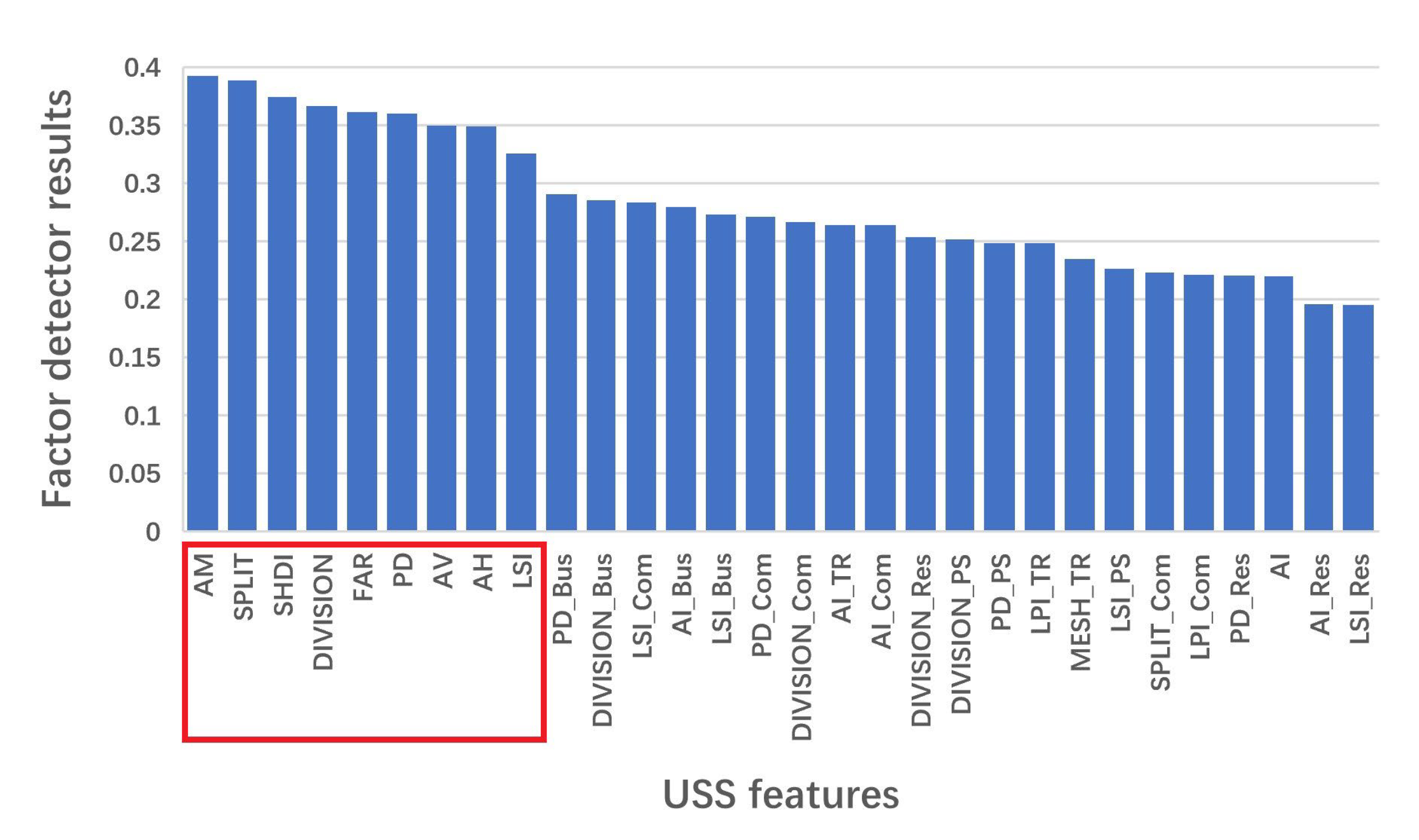
Figure 7 shows the 30 USS indicators with the strongest explanatory power for NTLI using the factor detector. The top nine consist of the landscape level indicator and 3D building form indicator, which are ranked as follows in terms of their explanatory power for the spatial heterogeneity of the NTLI: AM > SPLIT > SHDI > DIVISION > FAR > PD > AV > AH > LSI. Among all the indicators, AM is the factor that contributes the most to NTLI. Plots with large fluctuations in building height tend to have various features and types, typically accommodating more socioeconomic activities.

Figure 7.
The factor detector results of USS features on NTLI.
3.2.3. Interaction Detection of Diverse USS Factors on NTLI
Interaction detection was performed between a total of 14 factors at the landscape level and the built form level, and according to the results of the interaction detection, each pair of indicators enhanced the effect of the individual factors on NTLI in a binary enhanced or nonlinear enhanced form (Figure 8). Among these, q (SPLIT ∩ AV), q (PD ∩ AV), and q (AM ∩ AV) had the highest values of 0.595, 0.578, and 0.553, respectively.

Figure 8.
The interaction detector results of USS features on NTLI.
Table 4 presents the top ten q-values for the interaction detection results. It can be seen that although the interpretation rate of AA in factor detection is low, the interpretation rate, such as q (AA ∩ SPLIT) and q (AA ∩ AM), can increase the interpretation rate by more than 10% on a single factor basis. Among the top ten interaction q-values, eight resulted from the interaction between landscape pattern indicators and building form indicators. There are various landscape pattern indicators, while the building form indicators are mostly AV, indicating that combining urban landscape patterns and built form distribution is more powerful for explaining NTLI. Adjusting the pattern distribution of the functional structure of the city is an approach to socioeconomic development, especially in large cities with relatively saturated building heights and volumes.

Table 4.
Ten interaction detector results with the highest q-values.
3.3. Socioeconomic Benefits Evaluation of the Urban Spatial Structure
3.3.1. Model Construction
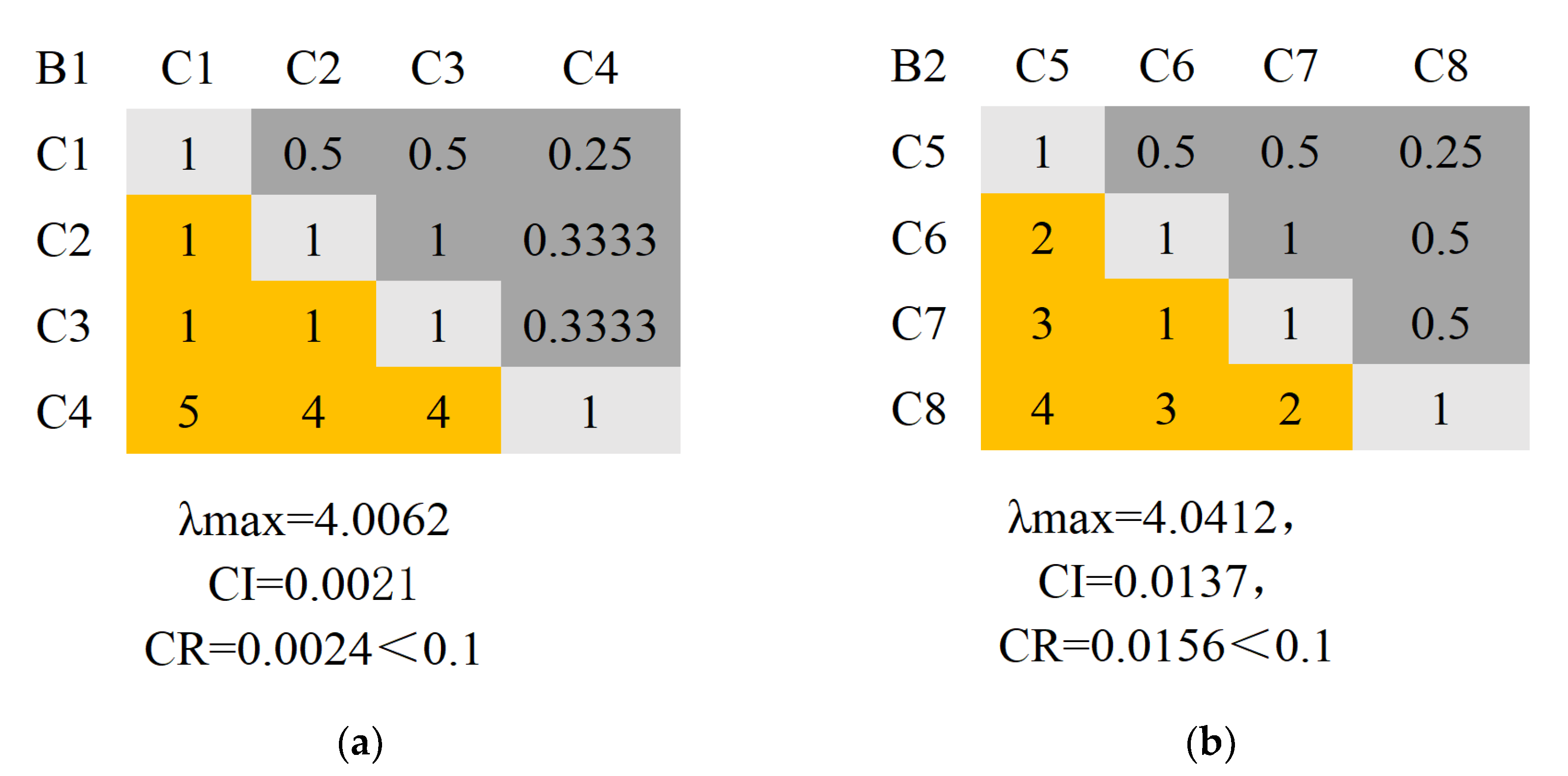
Considering the explanatory rate of USS on the factor detection of NTLI, we chose four landscape pattern indicators (B1) and four 3D building form indicators (B2) to construct the comparison matrix of evaluation indicators, including AH (C1), AV (C2), FAR (C3), AM (C4), PD (C5), DIVISION (C6), SHDI (C7), and SPLIT (C8). When the q-value of Ca is 0–0.1, 0.1–0.2, or 0.2–0.3 larger than that of Cb, the comparison matrix value of (Ca, Cb) is 2, 3, 4, and the value of (Cb, Ca) is 1/2, 1/3, 1/4, and so on. The corresponding comparison matrices were obtained based on the above principle, as illustrated in Figure 9. Finally, Table 5 presents the hierarchy of the model and calculated weights. Each factor must be normalized when calculating the weights to ensure that the calculated Spatial Structure Socioeconomic Benefit Index (SSSBI) is between 0 and 1.

Figure 9.
(a) Pairwise comparison matrix of building structures; (b) Pairwise comparison matrix of land-use function patterns.

Table 5.
Hierarchy and metric weight of SSSBI model.
In summary, the formula for SSSBI is as follows:
SSSBI = 0.0659 × AH + 0.0697 × AV + 0.0697 × FAR + 0.2948 × AM + 0.0483 × PD
+ 0.0967 × DIVISION + 0.1184 × SHDI + 0.2367 × SPLIT
+ 0.0967 × DIVISION + 0.1184 × SHDI + 0.2367 × SPLIT
3.3.2. SSSBI Distribution and Its Hot/Cold spots
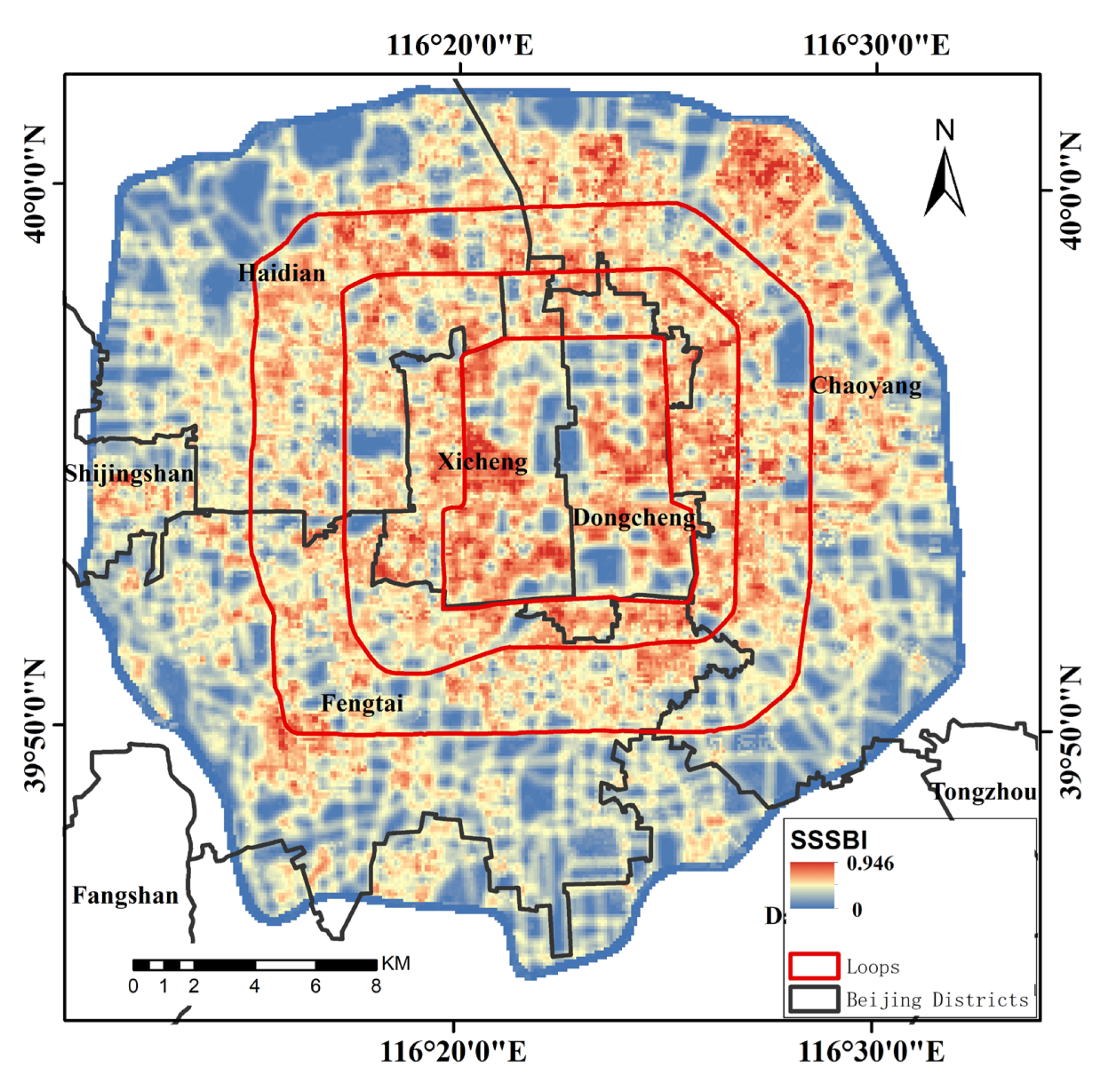
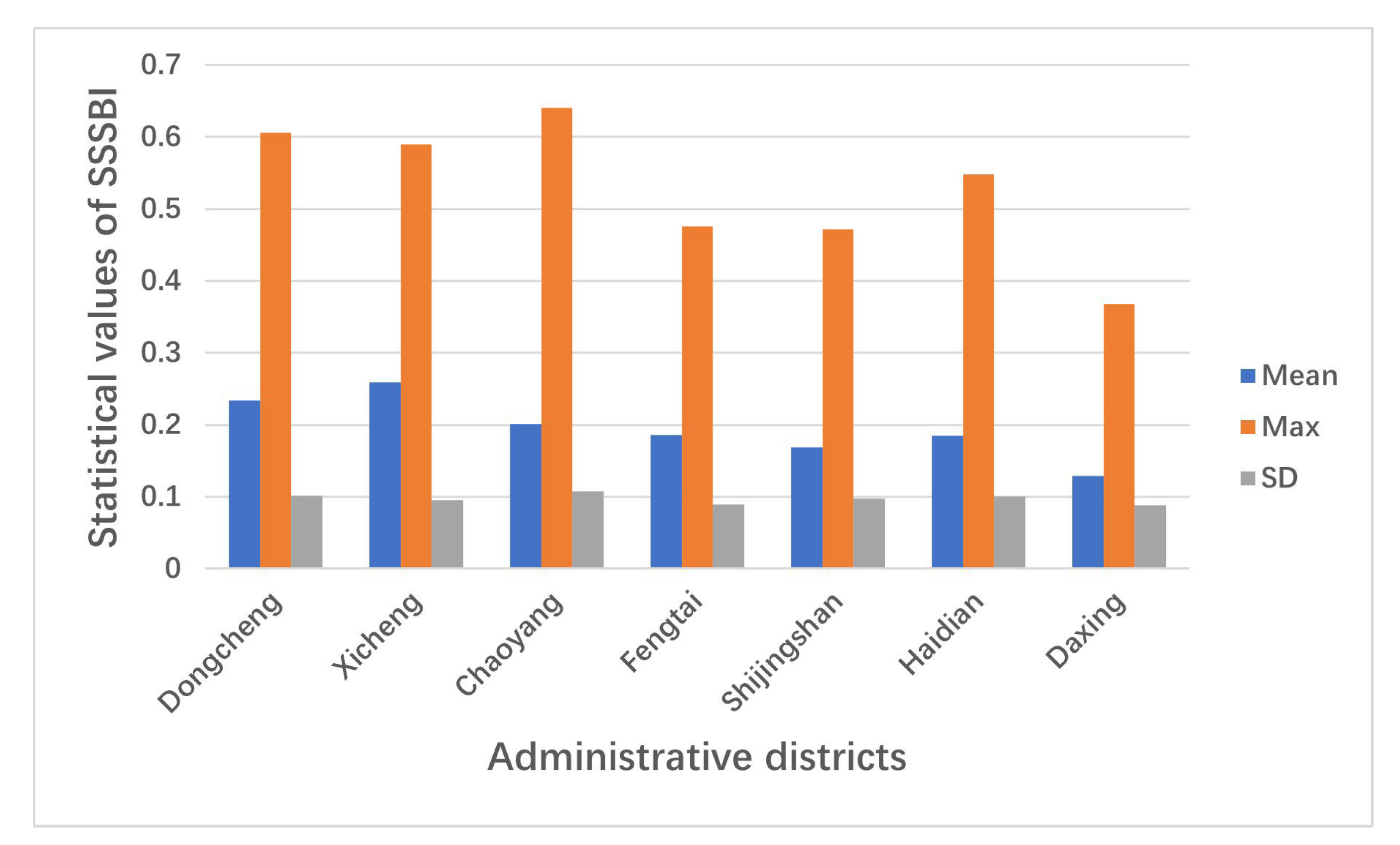
Figure 10 shows the SSSBI distribution. The SSSBI is highly spatially heterogeneous, with values decreasing from the center outwards according to the ring line. Figure 11 shows the statistical values of the mean, maximum (Max), and standard deviation (SD) of the SSSBI for different administrative districts. Dongcheng and Xicheng districts have the smallest mean values of SSSBI, indicating a relatively balanced overall urban socioeconomic development in both districts. Chaoyang District has the maximum SSSBI value, but its mean value is smaller than that of the Dongcheng and Xicheng Districts, and its standard deviation is larger, indicating that the Chaoyang District has a high level of socioeconomic development. However, the uneven distribution varies greatly within the region, and there may be hot spots.

Figure 10.
Spatial distributions of SSSBI.

Figure 11.
Mean, maximum (Max), and standard deviation (SD) of the SSSBI for different administrative districts within different administrative districts.
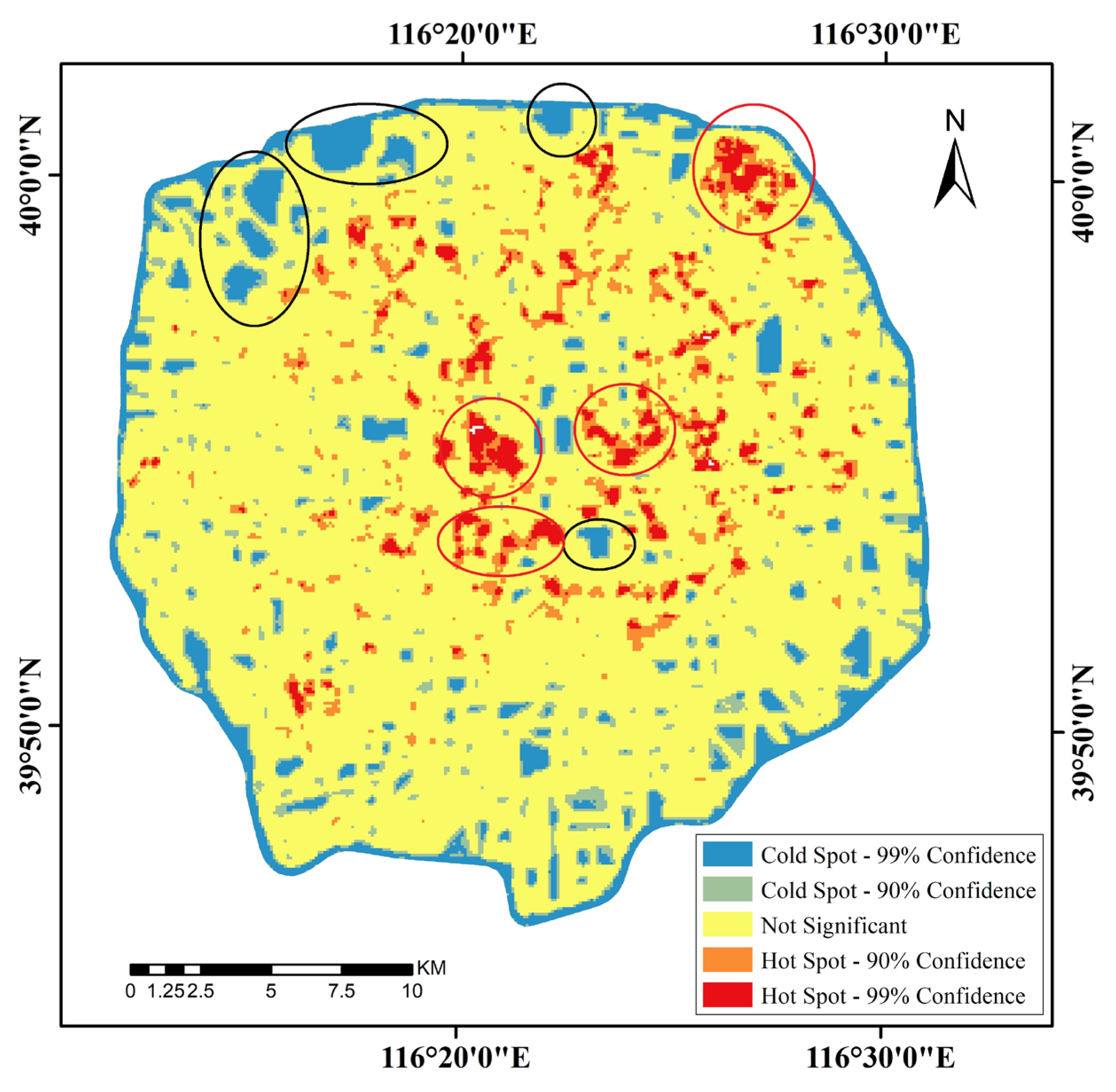
We represented the spatial distribution of statistically significant SSSBI high values (hot spots) and SSSBI low values (cold spots). The hot- and cold-spot regions with 90% and 99% confidence intervals are shown in Figure 12. Furthermore, four hot spots with z > 3.5 and four cold spots with z < –3 were found to focus on specific locations [60]. Three of the hotspots are located in the city’s central areas, and the cold spots are mainly located at the edges of the study area, all shown to be parks or recreational areas with abundant green areas. According to the order from west to east, the four cold spots are famous large parks in Beijing: The Summer Palace, Yuanmingyuan, Olympic Forest Park, and Tiantan Park. Referring to the Baidu map, the hotspot in the northeastern part of the study area is the Wangjing Development Zone in Chaoyang District, an important high-end international business and innovative urban complex in Beijing clustered with many commercial and business service facilities.
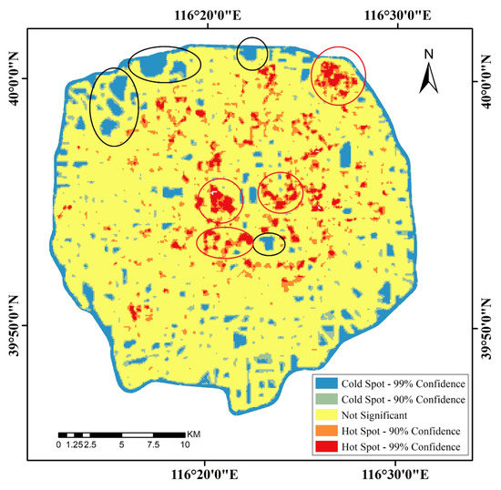
Figure 12.
Hot and cold spots of SSSBI. The red circle part is the hot spot area, and the black circle part is the cold spot area.
4. Discussion
4.1. Methodological Contributions
This study presents an exploratory method that combines urban spatial structure expressed based on physical environmental indicators with socioeconomic vitality levels reflected by nighttime brightness, aiming to explore the coupling relationship and driving benefits between USS and socioeconomic vitality levels. Few previous studies have considered the functional distribution of urban areas when calculating landscape indicators. This study combined high-resolution images and POI data to classify urban functional areas and obtain different functional landscape metrics of urban areas.
Furthermore, vertical urban expansion represented by the increase in high-rise buildings is an important feature of urban development. By integrating building surface data and height information, the 3D building form characteristics of the city were obtained and added to this study to construct a complete USS evaluation system.
In addition, the geographical detector was used for spatial statistical analysis. This study shows that the geo-detector can effectively study the different influencing factors and coupling effects between the USS and urban nighttime light intensity. Based on the results of the driving impact of USS features on UTL, an evaluation model of the USS was constructed. In contrast to previous evaluation models, this model considers the relationship and influence between the objective physical environment and socioeconomic factors of urban development, which is more objective and practical.
This study provides a valuable case framework for evaluating the urban spatial structure and its impact on socioeconomic dynamics. The SSSBI proposed based on an in-depth exploration of the relationship between USS and the socioeconomic environment. Landscape indicators and building form features can be used as an explanatory basis for evaluating USS.
4.2. Strategies for Optimizing Urban Spatial Structure Patterns
4.2.1. Correlation between USS and NTLI
From the results of this study, it can be concluded that the USS pattern is significantly correlated with NTLI, and different functional landscape and building form factors have different effects on NTLI. MESH and LPI in industrial areas are negatively related to NTLI, which is consistent with the findings of previous studies [61]. However, some studies found that increased industrial land in mountainous towns benefits socioeconomic development [62]. Our study noticed a weak negative correlation between SPLIT and NTLI in urban industrial areas. It is indicated that for cities in the early stage of urbanization, the increase in industrial land area is an essential positive driving force for socioeconomic development. In contrast, in large cities, the concentration of large industrial areas can impose certain constraints on the socioeconomic vitality of urban space. In conclusion, there are differences in the impact of the urban landscape on NTLI development under different city sizes and urbanization stages.
In addition, this study considers the diversity of the functional structure of a city based on the classification of the functional areas of the city. By analyzing SHDI and SPLIT indicators, we argue that an increase in the scale of urban buildings, the integrated enrichment of functions, and the decentralized distribution of different functional spaces can better enhance socioeconomic vitality.
4.2.2. Optimize the Spatial Structure at the Indicator Level
The socioeconomic benefits of USS are the result of the interaction between various urban land use functions and building forms. In factor detection, landscape-level metrics influence socioeconomic vitality more than class-level metrics. In interaction detection, the interactions among various landscape-level indicators were also found to enhance their impact on NTLI. This suggests that interactions between different functional landscape structures in the city enhance their effects on NTLI levels.
Factor detection also indicated that the impact of USS on NTLI was 3D metrics > 2D metrics. This was consistent with the findings of previous studies [63]. In addition, from the interaction detection results, the interaction between landscape form indicators and both 2D and 3D building form indicators could significantly increase the explanatory power of single indicators on NTLI. Therefore, the association between 3D building forms and socioeconomic levels should be valued, and the integrated consideration of 2D and 3D spatial structural features often allows for a more comprehensive exploration of their relationship with socioeconomic levels.
Therefore, from the perspective of the overall landscape pattern, increasing the type of the various functional areas could generate more socioeconomic benefits. In addition, the interaction of various drivers increases the driving force for the socioeconomic benefits of various structural indicators. The combination and overlay of multiple optimization approaches help improve the quality of the USS more comprehensively.
4.2.3. USS Quality Improvement in the SSSBI Cold Spots Region
The SSSBI assessment showed that most of the four cold spot areas are large green parks outside the 4th ring. The main element of these parks is their natural form, and the purpose of visitors is generally touring and ornamental. As a result, human activities in parks lack a strong intrinsic connection with the functions of the surrounding urban buildings. In addition, previous studies showed that parks have a significant effect on the average height of buildings. The closer to the park, the fewer high-rise buildings, inhibiting the surrounding socioeconomic activities to a certain extent [64]. Thus, the distribution pattern of large green parks can be optimized to improve the quality of USS and promote socioeconomic vitality.
The following recommendations can be made considering the experimental results of this study and actual local conditions:
- (1)
- Enrichment of the hierarchical structure of green spaces. Integrated planning of different types and scales of parks to build a hierarchical and comprehensive green space system. Large landscape parks could meet the needs of public excursions, and small green spaces could improve the accessibility of urban open spaces.
- (2)
- Strengthen night tour programs. Adding night tour projects can not only extend the tour time of visitors and increase the park’s capacity for same-day visitors but also attract visitors to shop and stay near the park. Gradually improve the night tour product system and promote the development of the tourism industry.
- (3)
- Introduce more urban public activities. Based on the open space and pleasant park environment, the internal site design was adjusted to transform the simple green garden into a green urban square with composite functions. Form a new model of diversified park tours combined with cultural experience, fitness and leisure, industrial sightseeing, and other themes.
4.3. Limitations
Unlike evaluations based on subjective perceptions, this study uses a geographic detector to research the impact of USS on socioeconomics, which helps to develop evaluation indicators more objectively. Nevertheless, this study had some limitations.
The technological innovation of experimental methods is very important. In future studies, it is necessary to further improve the neural network structure of functional area classification by combining multimodal data sources while selecting more refined samples. Furthermore, there is a need to increase the innovativeness and generalizability of data analysis methods.
In addition, a variety of network data sources, such as POI data and OSM data, were used in this study. Although preprocessing is done before use, category confusion and data redundancy may still exist due to the huge amount of data and diverse categories. Therefore, improving the accuracy of the data remains an important issue. In future research, more effective data preprocessing methods should be studied to enhance the accuracy of data and the reliability of results.
This study focused only on Beijing. However, under different urban scales and urban development stages, not only do the urban landscape and functions vary greatly, but also the distribution characteristics of building forms. In future research, we look forward to exploring mechanisms and adaptive analysis through more case studies, finding several general indicators for evaluating USS through more case studies, and specifying which indicators can be used specifically when the spatial structure of a study area meets which conditions.
5. Conclusions
Urbanization has led to a series of urban problems, and the rational layout of the USS plays an essential role in promoting urban development. Different landscape patterns and building forms in USS give rise to different socioeconomic benefits. In this context, this study investigates the effects of different functional urban landscape patterns and 3D-building forms on the socioeconomic benefits of urban areas using a geographic detector that describes their features on a multi-scale basis and establishes an objective and quantitative assessment model of USS, which has important practical implications for the planning and optimization of USS. Based on the results of this study, the following conclusions were drawn.
First, by analyzing the fitting results of USS features and NTLI at different statistical scales, it was found that the fitting accuracy of USS and NTLI varied significantly with scales up to 1400 m, while the scale factor had little influence on the fitting results of USS and NTLI beyond 1400 m. Therefore, adopting an evaluation scale of 1400 m is helpful for systematically evaluating the socioeconomic benefits of urban spatial structures.
Second, the explanatory power of landscape-level factors in the landscape pattern index is higher than that of category-level factors in evaluating the socioeconomic benefits of USS; the explanatory power of 3D indicators in the building form index is higher than that of 2D indicators. Spatial structure patterns with high land utilization and comprehensive and compact functions are more conducive to developing socioeconomic activities.
Third, the combined effect of any two spatial structure factors on NTLI is higher than the effect of each factor. The level of urban spatial structure distribution can be improved from multiple perspectives, such as integrating 2D and 3D spatial structures, enhancing the combination of various spatial structural forms, and increasing the diversity of urban functions, especially in developed cities where the development of built spaces has reached its peak.
Fourth, this study quantitatively evaluates the quality of USS based on SSSBI and identifies four large park green space areas in the study area that need structural optimization in combination with cold spot analysis, providing strategies for urban quality assessment and development planning.
Due to data and technical limitations, this paper still has some limitations. However, the findings still emphasize the importance of focusing on the impact mechanisms of socioeconomic benefits of USS to improve the urban structure and enhance livability. Further investigation into the effects of more detailed and diverse USS characteristics is warranted. A mechanism exploration and adaptability analysis based on multiple city experiments is also needed.
Author Contributions
Conceptualization, Y.L. and Q.M.; methodology, Y.L.; software and writing—original draft, Y.L.; data curation, Y.L. and Q.M.; writing—review and editing, Y.L., Q.M., J.Z., L.Z., M.A., X.H. and C.Z.; visualization, Y.L.; supervision, Q.M.; funding acquisition, Q.M. All authors have read and agreed to the published version of the manuscript.
Funding
This research was funded by the National Key Research and Development Program of China, grant number 2020YFC0833100; the research on the multi-perspective evaluation of urban green space based on remote sensing and street view data, grant number 42171357; Study on the spatial-temporal heterogeneity of urban anthropogenic heat and its environmental effects simulation in multi-scenes, grant number 42201384.
Data Availability Statement
The data presented in this study are available on request from the corresponding website.
Conflicts of Interest
The authors declare no conflict of interest.
References
- Hoekstra, A.Y.; Wiedmann, T.O. Humanity’s Unsustainable Environmental Footprint. Science 2014, 344, 1114–1117. [Google Scholar] [CrossRef] [PubMed]
- Bhatta, B. Analysis of Urban Growth and Sprawl from Remote Sensing Data; Advances in Geographic Information Science; Springer: Heidelberg, Germany; New York, NY, USA, 2010; ISBN 978-3-642-05298-9. [Google Scholar]
- Al-Mulali, U.; Ozturk, I.; Lean, H.H. The Influence of Economic Growth, Urbanization, Trade Openness, Financial Development, and Renewable Energy on Pollution in Europe. Nat. Hazards 2015, 79, 621–644. [Google Scholar] [CrossRef]
- Bai, X.; Chen, J.; Shi, P. Landscape Urbanization and Economic Growth in China: Positive Feedbacks and Sustainability Dilemmas. Environ. Sci. Technol. 2012, 46, 132–139. [Google Scholar] [CrossRef] [PubMed]
- Clark, D. Book Review: Internal Structure of the City: Readings on Urban Growth, form and Policy. Prog. Hum. Geogr. 1984, 8, 453–455. [Google Scholar] [CrossRef]
- Bourne, L.S. Internal Structure of the City: Readings on Urban Form, Growth, and Policy; Oxford University Press: New York, NY, USA, 1982. [Google Scholar]
- Angel, S.; Parent, J.; Civco, D.L.; Blei, A.; Potere, D. The Dimensions of Global Urban Expansion: Estimates and Projections for All Countries, 2000–2050. Prog. Plan. 2011, 75, 53–107. [Google Scholar] [CrossRef]
- Chong, Z.; Qin, C.; Ye, X. Environmental Regulation and Industrial Structure Change in China: Integrating Spatial and Social Network Analysis. Sustainability 2017, 9, 1465. [Google Scholar] [CrossRef]
- Deng, X.; Huang, J.; Rozelle, S.; Uchida, E. Economic Growth and the Expansion of Urban Land in China. Urban Stud. 2010, 47, 813–843. [Google Scholar] [CrossRef]
- De Espindola, G.M.; da Costa Carneiro, E.L.N.; Façanha, A.C. Four Decades of Urban Sprawl and Population Growth in Teresina, Brazil. Appl. Geogr. 2017, 79, 73–83. [Google Scholar] [CrossRef]
- Buhaug, H.; Urdal, H. An Urbanization Bomb? Population Growth and Social Disorder in Cities. Glob. Environ. Chang. 2013, 23, 1–10. [Google Scholar] [CrossRef]
- Huang, X.; Wang, Y. Investigating the Effects of 3D Urban Morphology on the Surface Urban Heat Island Effect in Urban Functional Zones by Using High-Resolution Remote Sensing Data: A Case Study of Wuhan, Central China. ISPRS J. Photogramm. Remote Sens. 2019, 152, 119–131. [Google Scholar] [CrossRef]
- Chen, Z.; Yu, B.; Song, W.; Liu, H.; Wu, Q.; Shi, K.; Wu, J. A New Approach for Detecting Urban Centers and Their Spatial Structure With Nighttime Light Remote Sensing. IEEE Trans. Geosci. Remote Sens. 2017, 55, 6305–6319. [Google Scholar] [CrossRef]
- Zhang, Q.; Seto, K.C. Mapping Urbanization Dynamics at Regional and Global Scales Using Multi-Temporal DMSP/OLS Nighttime Light Data. Remote Sens. Environ. 2011, 115, 2320–2329. [Google Scholar] [CrossRef]
- Li, Q.; Zheng, H.; Zhang, G.; Guo, X.; Liu, W. Analysis of luojia1-01 index based on nighttime light imagery. J. Geomat. 2020, 45, 8–15. [Google Scholar] [CrossRef]
- Yu, B.; Lian, T.; Huang, Y.; Yao, S.; Ye, X.; Chen, Z.; Yang, C.; Wu, J. Integration of Nighttime Light Remote Sensing Images and Taxi GPS Tracking Data for Population Surface Enhancement. Int. J. Geogr. Inf. Sci. 2019, 33, 687–706. [Google Scholar] [CrossRef]
- Jean, N.; Burke, M.; Xie, M.; Davis, W.M.; Lobell, D.B.; Ermon, S. Combining Satellite Imagery and Machine Learning to Predict Poverty. Science 2016, 353, 790–794. [Google Scholar] [CrossRef]
- Tan, Z.; Wei, D.; Yin, Z. Housing Vacancy Rate in Major Cities in China: Perspectives from Nighttime Light Data. Complexity 2020, 2020, 5104578. [Google Scholar] [CrossRef]
- Elvidge, C.D.; Baugh, K.E.; Kihn, E.A.; Kroehl, H.W.; Davis, E.R.; Davis, C.W. Relation between Satellite Observed Visible-near Infrared Emissions, Population, Economic Activity and Electric Power Consumption. Int. J. Remote Sens. 1997, 18, 1373–1379. [Google Scholar] [CrossRef]
- Liu, Y.; Liu, X.; Gao, S.; Gong, L.; Kang, C.; Zhi, Y.; Chi, G.; Shi, L. Social Sensing: A New Approach to Understanding Our Socioeconomic Environments. Ann. Assoc. Am. Geogr. 2015, 105, 512–530. [Google Scholar] [CrossRef]
- Li, D.R. Towards geo-spatial information science in big data era. Acta Geod. Cartogr. Sin. 2016, 45, 379–384. [Google Scholar] [CrossRef]
- Shan, J.; Qin, K.; Huang, C.Q.; Hu, X.Y.; Yu, Y.; Hu, Q.W.; Lin, Z.Y.; Chen, J.P.; Jia, T. Methods of Crowd Sourcing Geographic Data Processing and Analysis. Geomat. Inf. Sci. Wuhan Univ. 2014, 39, 390–396. [Google Scholar] [CrossRef]
- Wang, X.; Meng, Q.; Zhang, L.; Hu, D. Evaluation of urban green space in terms of thermal environmental benefits using geographical detector analysis. Int. J. Appl. Earth Obs. Geoinf. 2021, 105, 102610. [Google Scholar] [CrossRef]
- Wang, B.; Liu, Z.; Mei, Y.; Li, W. Assessment of Ecosystem Service Quality and Its Correlation with Landscape Patterns in Haidian District, Beijing. Int. J. Environ. Res. Public Health 2019, 16, 1248. [Google Scholar] [CrossRef] [PubMed]
- Yu, B.; Shu, S.; Liu, H.; Song, W.; Wu, J.; Wang, L.; Chen, Z. Object-Based Spatial Cluster Analysis of Urban Landscape Pattern Using Nighttime Light Satellite Images: A Case Study of China. Int. J. Geogr. Inf. Sci. 2014, 28, 2328–2355. [Google Scholar] [CrossRef]
- Huang, X.; Hu, T.; Li, J.; Wang, Q.; Benediktsson, J.A. Mapping Urban Areas in China Using Multisource Data With a Novel Ensemble SVM Method. IEEE Trans. Geosci. Remote Sens. 2018, 56, 4258–4273. [Google Scholar] [CrossRef]
- Liu, X. Mapping Urban Extent at Large Spatial Scales Using Machine Learning Methods with VIIRS Nighttime Light and MODIS Daytime NDVI Data. Remote Sens. 2019, 11, 1247. [Google Scholar] [CrossRef]
- Yu, L.; Wang, J.; Gong, P. Improving 30 m Global Land-Cover Map FROM-GLC with Time Series MODIS and Auxiliary Data Sets: A Segmentation-Based Approach. Int. J. Remote Sens. 2013, 34, 5851–5867. [Google Scholar] [CrossRef]
- Tian, Y. The Effect of Urban 2D and 3D Morphology on Air Temperature in Residential Neighborhoods. Landsc. Ecol. 2019, 34, 1161–1178. [Google Scholar] [CrossRef]
- Small, C. Multisensor Characterization of Urban Morphology and Network Structure. Remote Sens. 2019, 11, 2162. [Google Scholar] [CrossRef]
- Chen, K.; Zou, Z.; Shi, Z. Building Extraction from Remote Sensing Images with Sparse Token Transformers. Remote Sens. 2021, 13, 4441. [Google Scholar] [CrossRef]
- Chen, M.; Wu, J.; Liu, L.; Zhao, W.; Tian, F.; Shen, Q.; Zhao, B.; Du, R. DR-Net: An Improved Network for Building Extraction from High Resolution Remote Sensing Image. Remote Sens. 2021, 13, 294. [Google Scholar] [CrossRef]
- Lv, N.; Zhang, Z.; Li, C.; Deng, J.X.; Su, T.; Chen, C. A hybrid-attention semantic segmentation network for remote sensing interpretation in land-use surveillance. Int. J. Mach. Learn. Cyber. 2022. [Google Scholar] [CrossRef]
- Wang, J.; Hu, X.; Meng, Q.; Zhang, L.; Wang, C.; Liu, X.; Zhao, M. Developing a Method to Extract Building 3D Information from GF-7 Data. Remote Sens. 2021, 13, 4532. [Google Scholar] [CrossRef]
- Bullinger, S.; Bodensteiner, C.; Arens, M. 3D Surface Reconstruction From Multi-Date Satellite Images. arXiv 2021, arXiv:2102.02502. [Google Scholar] [CrossRef]
- Wu, B.; Yu, B.; Wu, Q.; Chen, Z.; Yao, S.; Huang, Y.; Wu, J. An Extended Minimum Spanning Tree Method for Characterizing Local Urban Patterns. Int. J. Geogr. Inf. Sci. 2018, 32, 450–475. [Google Scholar] [CrossRef]
- Xie, J.; Feng, C.-C. An Integrated Simplification Approach for 3D Buildings with Sloped and Flat Roofs. IJGI 2016, 5, 128. [Google Scholar] [CrossRef]
- Zhang, P.F.; Hu, Y.M.; Xiong, Z.P. Variation pattern and its affecting factors of three-dimensional landscape in urban residential community of Shenyang. Chin. J. Appl. Ecol. 2011, 2011, 453–459. [Google Scholar] [CrossRef]
- Wu, Q.; Guo, F.X.; Li, H.Q.; Kang, J.Y. Measuring landscape pattern in three dimensional space. Landsc. Urban Plan. 2017, 167, 49–59. [Google Scholar] [CrossRef]
- Long, Y.; Li, P.; Hou, J.X. Three-dimensional Urban Form at the Street Block Level for Major Cities in China. Shanghai Urban Plan. Rev. 2019, 3, 1673–8985. [Google Scholar] [CrossRef]
- Bennett, M.M.; Smith, L.C. Advances in Using Multitemporal Night-Time Lights Satellite Imagery to Detect, Estimate, and Monitor Socioeconomic Dynamics. Remote Sens. Environ. 2017, 192, 176–197. [Google Scholar] [CrossRef]
- Wang, L.; Fan, H.; Wang, Y. Improving Population Mapping Using Luojia 1-01 Nighttime Light Image and Location-Based Social Media Data. Sci. Total Environ. 2020, 730, 139148. [Google Scholar] [CrossRef]
- Chen, Z.; Yu, B.; Hu, Y.; Huang, C.; Shi, K.; Wu, J. Estimating House Vacancy Rate in Metropolitan Areas Using NPP-VIIRS Nighttime Light Composite Data. IEEE J. Sel. Top. Appl. Earth Obs. Remote Sens. 2015, 8, 2188–2197. [Google Scholar] [CrossRef]
- Venkatalaxmi, A.; Padmavathi, B.S.; Amaranath, T. A General Solution of Unsteady Stokes Equations. Fluid Dyn. Res. 2004, 35, 229–236. [Google Scholar] [CrossRef]
- Zhao, X.; Yu, B.; Liu, Y.; Chen, Z.; Li, Q.; Wang, C.; Wu, J. Estimation of Poverty Using Random Forest Regression with Multi-Source Data: A Case Study in Bangladesh. Remote Sens. 2019, 11, 375. [Google Scholar] [CrossRef]
- Shi, K.; Chen, Y.; Yu, B.; Xu, T.; Yang, C.; Li, L.; Huang, C.; Chen, Z.; Liu, R.; Wu, J. Detecting Spatiotemporal Dynamics of Global Electric Power Consumption Using DMSP-OLS Nighttime Stable Light Data. Appl. Energy 2016, 184, 450–463. [Google Scholar] [CrossRef]
- Shi, K.; Chen, Y.; Yu, B.; Xu, T.; Chen, Z.; Liu, R.; Li, L.; Wu, J. Modeling Spatiotemporal CO2 (Carbon Dioxide) Emission Dynamics in China from DMSP-OLS Nighttime Stable Light Data Using Panel Data Analysis. Appl. Energy 2016, 168, 523–533. [Google Scholar] [CrossRef]
- Zhang, X.; Du, S.; Du, S.; Liu, B. How Do Land-Use Patterns Influence Residential Environment Quality? A Multiscale Geographic Survey in Beijing. Remote Sens. Environ. 2020, 249, 112014. [Google Scholar] [CrossRef]
- Chen, X.; Nordhaus, W.D. Using Luminosity Data as a Proxy for Economic Statistics. Proc. Natl. Acad. Sci. USA 2011, 108, 8589–8594. [Google Scholar] [CrossRef]
- Chen, C.; Fushing, H. Multiscale Community Geometry in a Network and Its Application. Phys. Rev. E 2012, 86, 041120. [Google Scholar] [CrossRef]
- Mcgarigal, K.S.; Cushman, S.A.; Neel, M.C. Spatial Pattern Analysis Program for Categorical Maps. Fragstats. 2002. Available online: www.umass.edu/landeco/research/fragstats/fragstats.html (accessed on 3 March 2021).
- Wang, J.; Li, X.; Christakos, G.; Liao, Y.; Zhang, T.; Gu, X.; Zheng, X. Geographical Detectors-Based Health Risk Assessment and Its Application in the Neural Tube Defects Study of the Heshun Region, China. Int. J. Geogr. Inf. Sci. 2010, 24, 107–127. [Google Scholar] [CrossRef]
- Zhao, X.; Liu, J.; Hao, H.; Yang, Y. Quantifying the Spatial Heterogeneity and Driving Factors of Aboveground Forest Biomass in the Urban Area of Xi’an, China. ISPRS Int. J. Geo-Inf. 2020, 9, 744. [Google Scholar] [CrossRef]
- Zhao, X.; Liu, J.; Bu, Y. Quantitative Analysis of Spatial Heterogeneity and Driving Forces of the Thermal Environment in Urban Built-up Areas: A Case Study in Xi’an, China. Sustainability 2021, 13, 1870. [Google Scholar] [CrossRef]
- Breiman, L. Bagging Predictors. Mach. Learn. 1996, 24, 123–140. [Google Scholar] [CrossRef]
- Statistics, L.B.; Breiman, L. Random Forests. Mach. Learn. 2001, 45, 5–32. [Google Scholar] [CrossRef]
- Kordi, M.; Brandt, S.A. Effects of Increasing Fuzziness on Analytic Hierarchy Process for Spatial Multicriteria Decision Analysis. Comput. Environ. Urban Syst. 2012, 36, 43–53. [Google Scholar] [CrossRef]
- Parsian, S.; Amani, M.; Moghimi, A.; Ghorbanian, A.; Mahdavi, S. Flood Hazard Mapping Using Fuzzy Logic, Analytical Hierarchy Process, and Multi-Source Geospatial Datasets. Remote Sens. 2021, 13, 4761. [Google Scholar] [CrossRef]
- Saaty, T.L. Decision Making—The Analytic Hierarchy and Network Processes (AHP/ANP). J. Syst. Sci. Syst. Eng. 2004, 13, 1–35. [Google Scholar] [CrossRef]
- Fan, P.; Xu, L.; Yue, W.; Chen, J. Accessibility of Public Urban Green Space in an Urban Periphery: The Case of Shanghai. Landsc. Urban Plan. 2017, 165, 177–192. [Google Scholar] [CrossRef]
- Zhang, H.; Hu, Q.; Zhang, Y. Vertical decentralization and horizontal competition: How administrative governance models affect the coordinated development of urbanization and industrialization in prefecture-level cities. Financ. Trade Econ. 2022, 43, 112–127. [Google Scholar] [CrossRef]
- Zheng, L.; Li, Z.; Li, P.; Gao, H.; Xu, G.; Ke, H. Simulation of landscape pattern and socio-economic response relationship in the Danjiang Tusk Mountains. Soil Water Conserv. Res. 2019, 26, 338–343. [Google Scholar] [CrossRef]
- Wang, C.; Chen, Z.; Yang, C.; Li, Q.; Wu, Q.; Wu, J.; Zhang, G.; Yu, B. Analyzing Parcel-Level Relationships between Luojia 1-01 Nighttime Light Intensity and Artificial Surface Features across Shanghai, China: A Comparison with NPP-VIIRS Data. Int. J. Appl. Earth Obs. Geoinf. 2020, 85, 101989. [Google Scholar] [CrossRef]
- Zhang, P.; Song, Y.; Liu, J.; Gao, Y.; Li, X. Analysis of influencing factors of urban three-dimensional architectural landscape. Urban Archit. 2019, 16, 135–139. [Google Scholar] [CrossRef]
Publisher’s Note: MDPI stays neutral with regard to jurisdictional claims in published maps and institutional affiliations. |
© 2022 by the authors. Licensee MDPI, Basel, Switzerland. This article is an open access article distributed under the terms and conditions of the Creative Commons Attribution (CC BY) license (https://creativecommons.org/licenses/by/4.0/).

