Spatial Effects of Landscape Patterns of Urban Patches with Different Vegetation Fractions on Urban Thermal Environment
Abstract
1. Introduction
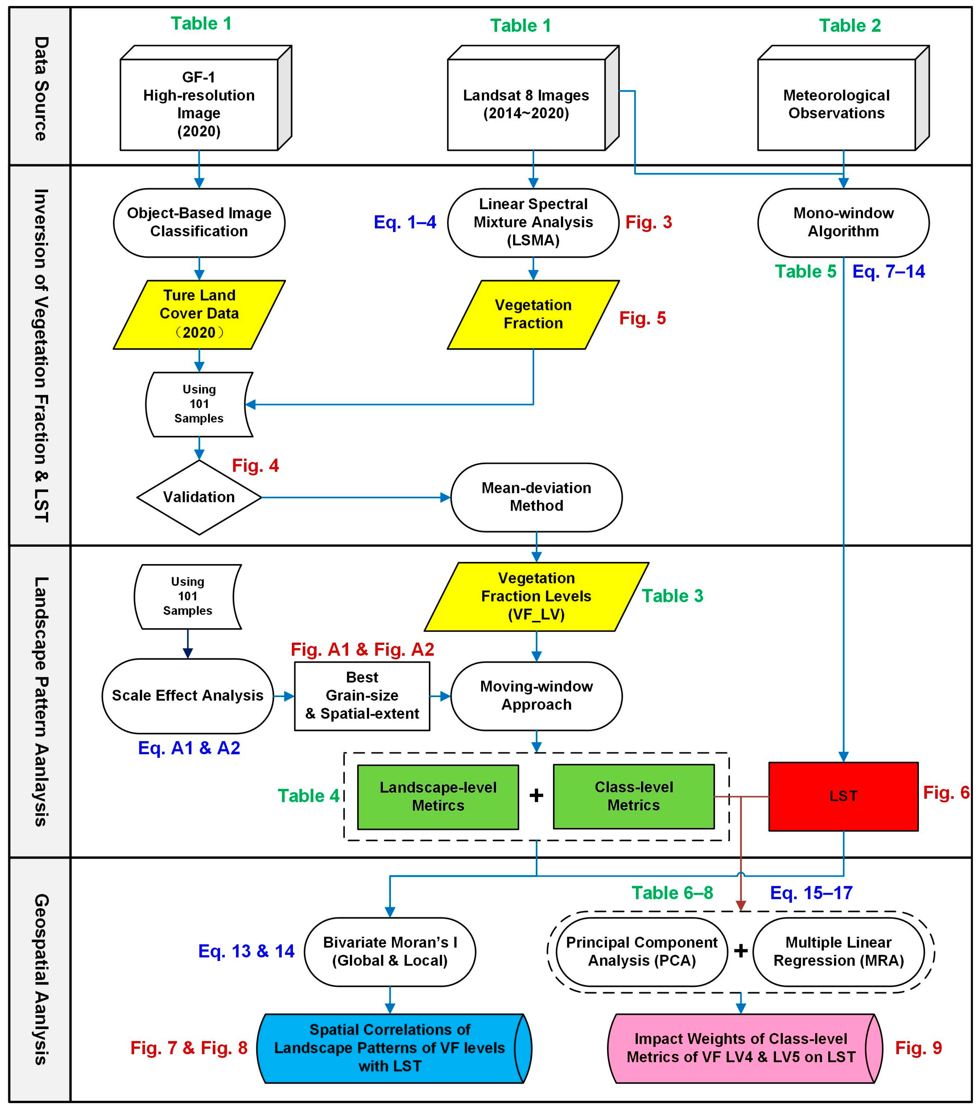
2. Materials and Methods
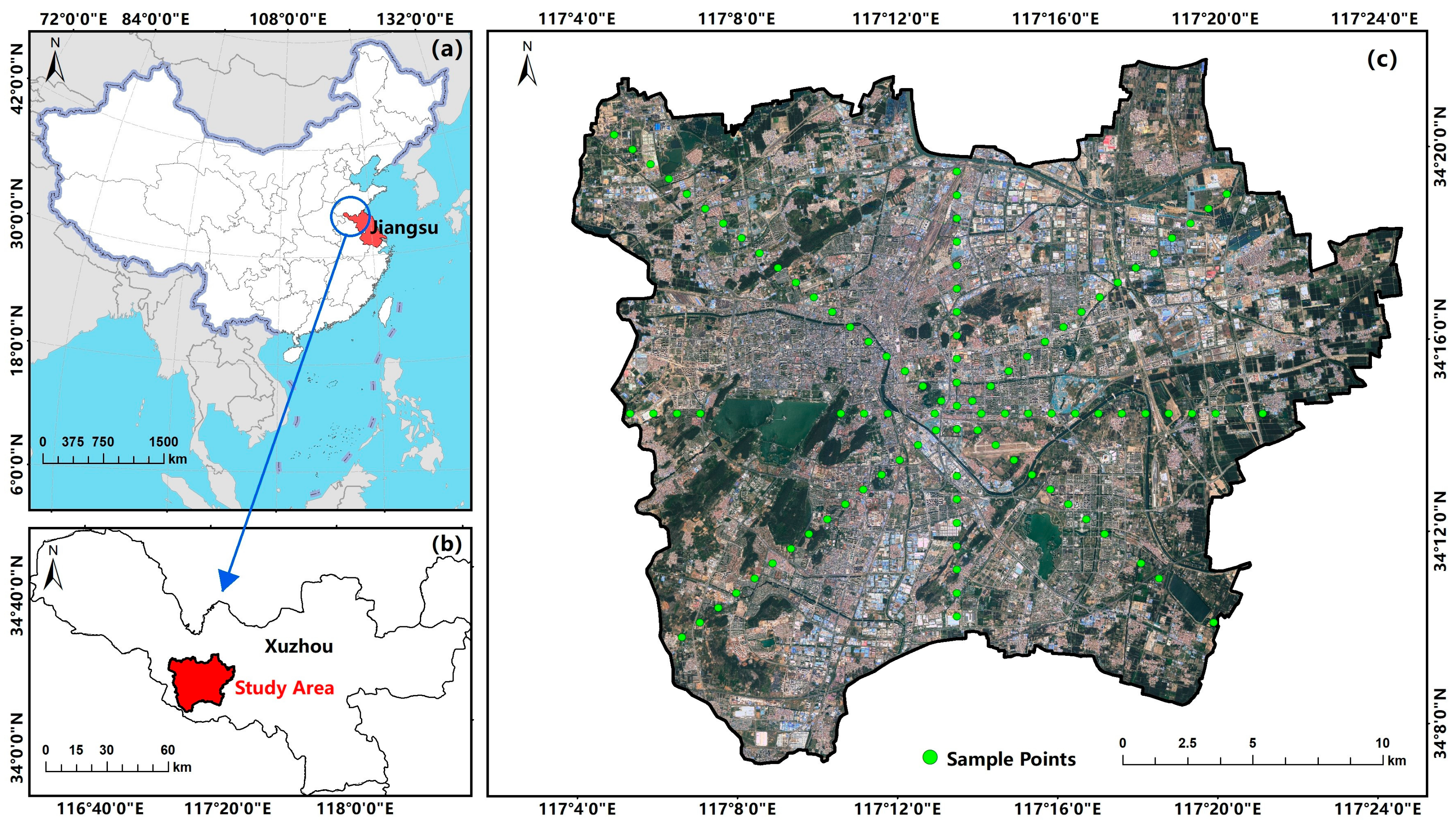
2.1. Study Area
2.2. Data Descriptions
2.2.1. Satellite Data
2.2.2. Ground Observations
2.3. Extraction of Vegetation Fraction from Mixed Pixels
2.3.1. Selection of Spectral Mixture Analysis Model
2.3.2. Extraction of Endmember Fraction
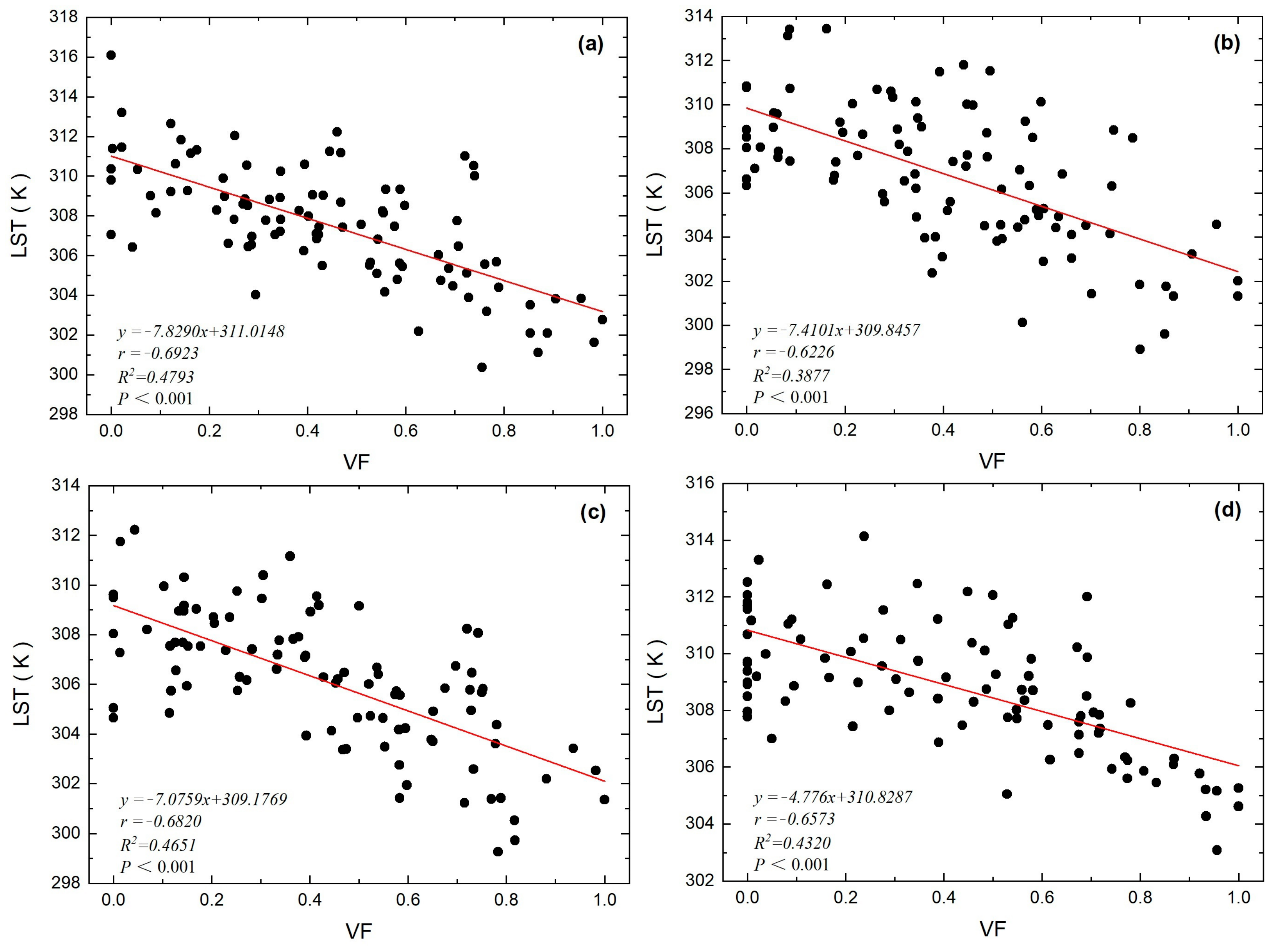
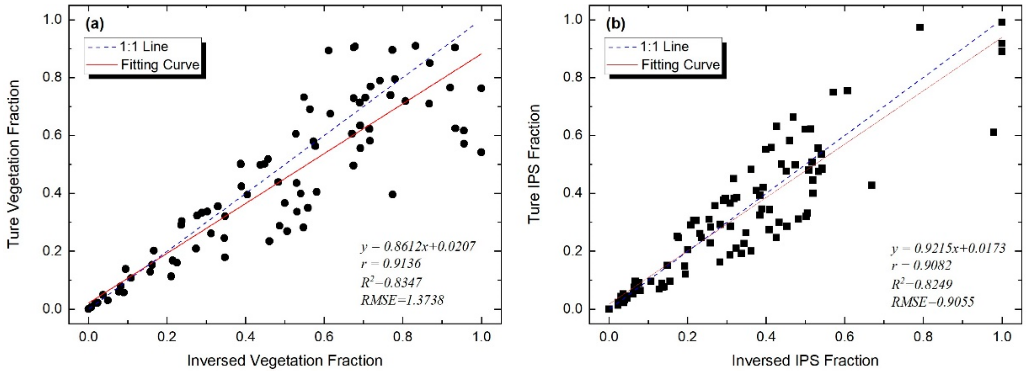
2.3.3. Validation of Endmember Fraction
2.4. Analysis of Vegetation Fraction Levels Using Landscape Metrics
2.4.1. Definitions of Vegetation Fraction Levels
2.4.2. Selection of Landscape Metrics
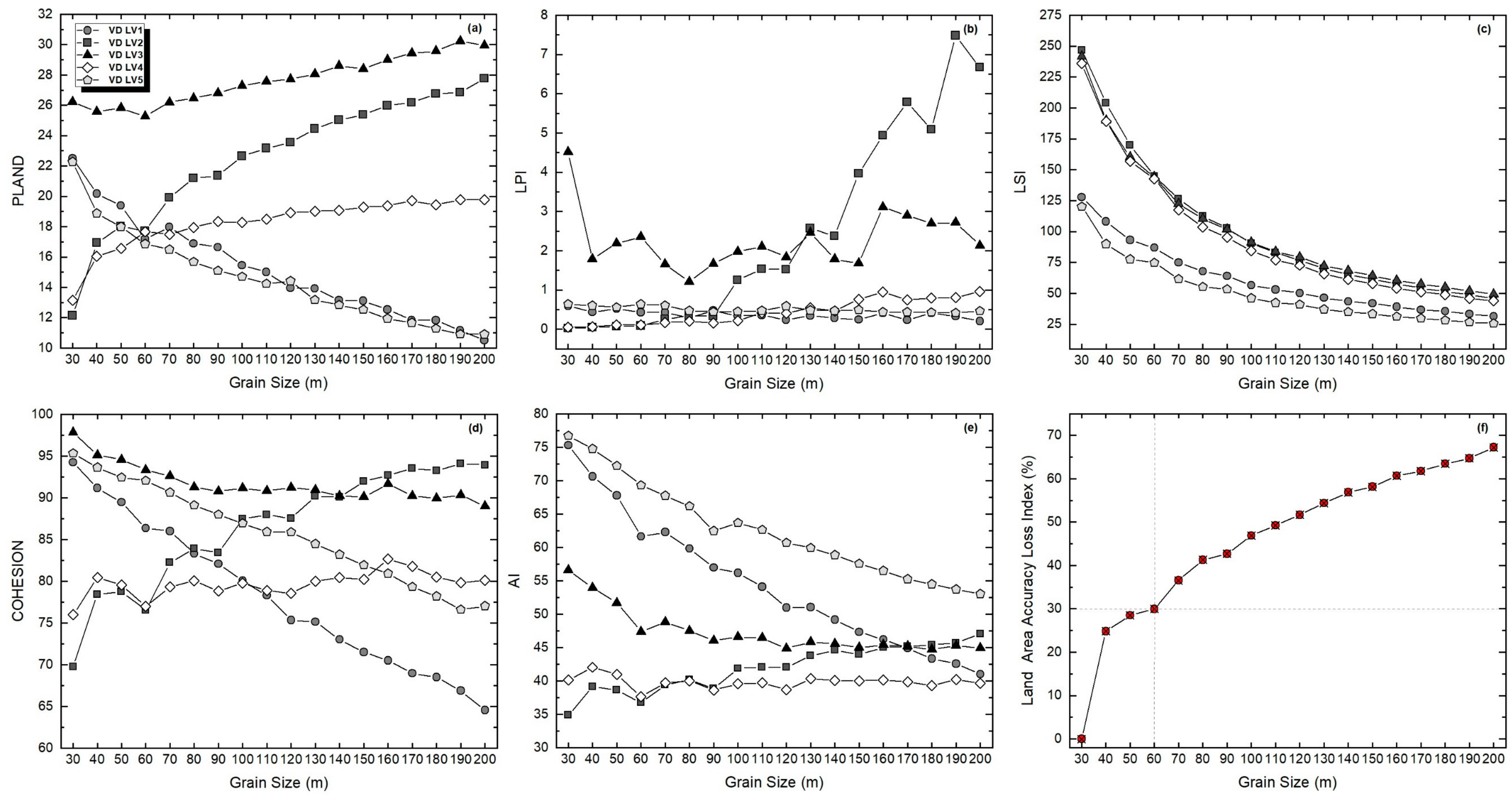
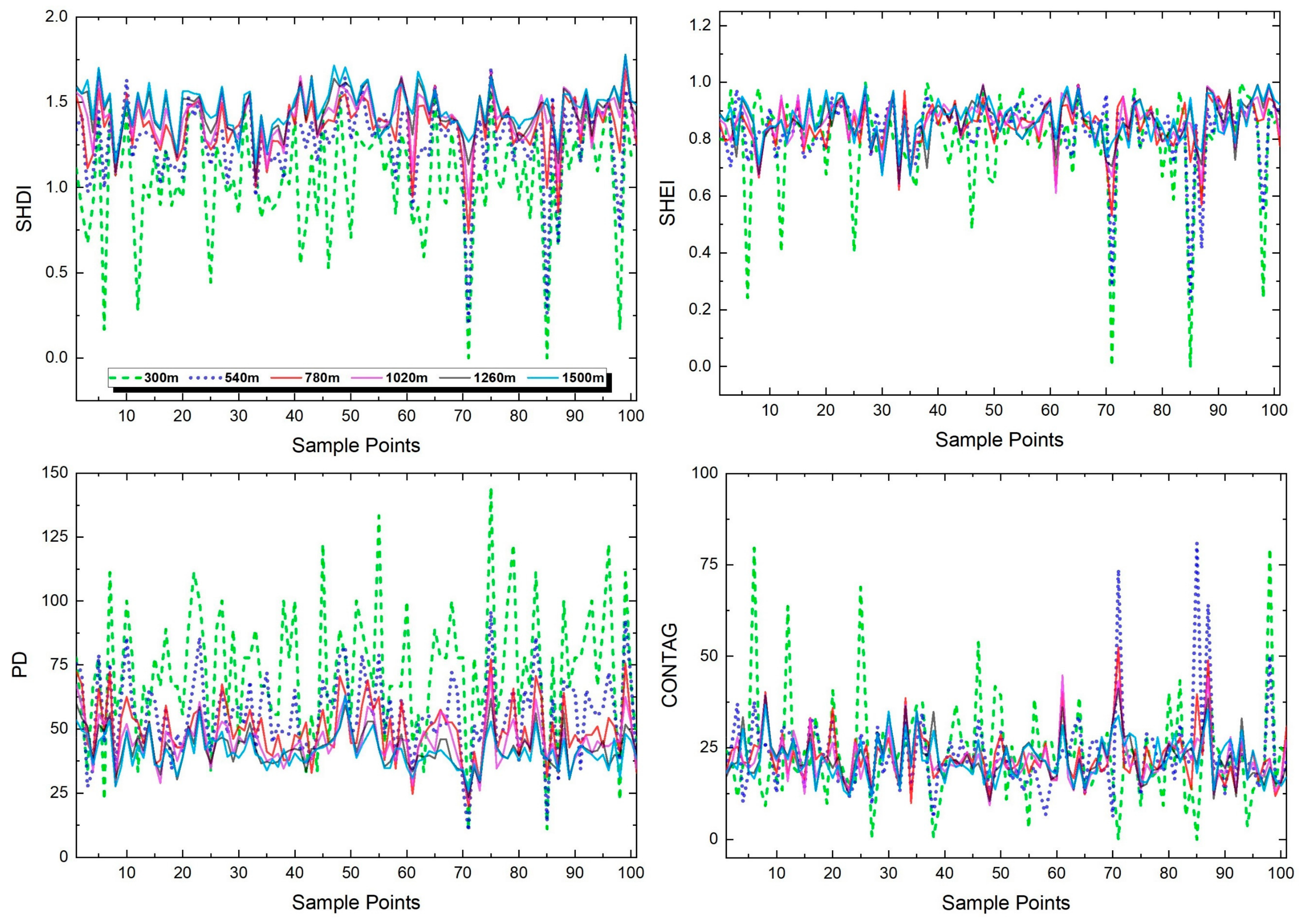
2.4.3. Scale Effect Analysis
2.5. Landscape Surface Temperature Inversion
2.6. Spatial Correlation Analysis
2.7. Impact Weight Calculation Based on Principal Component Analysis
3. Results
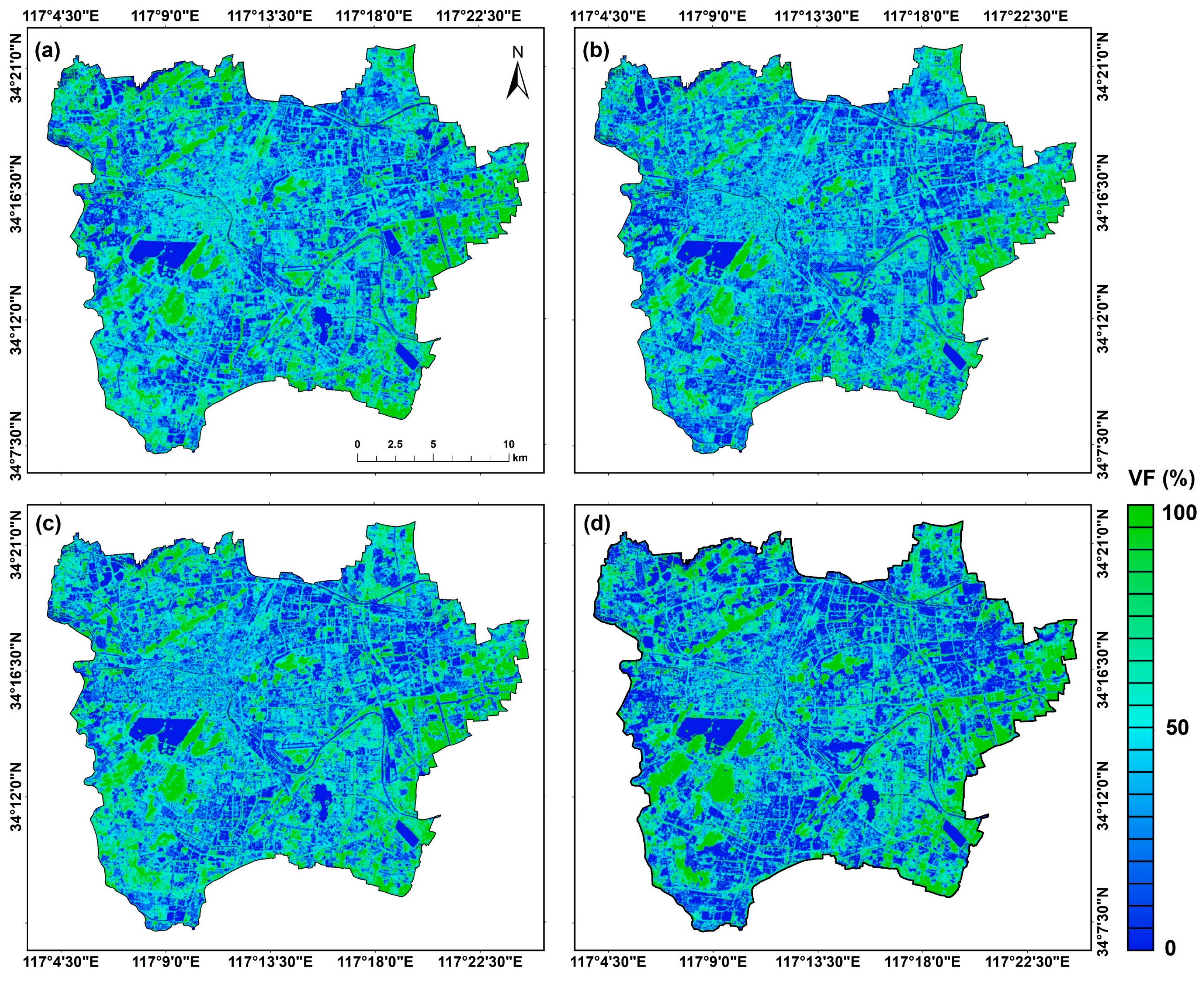
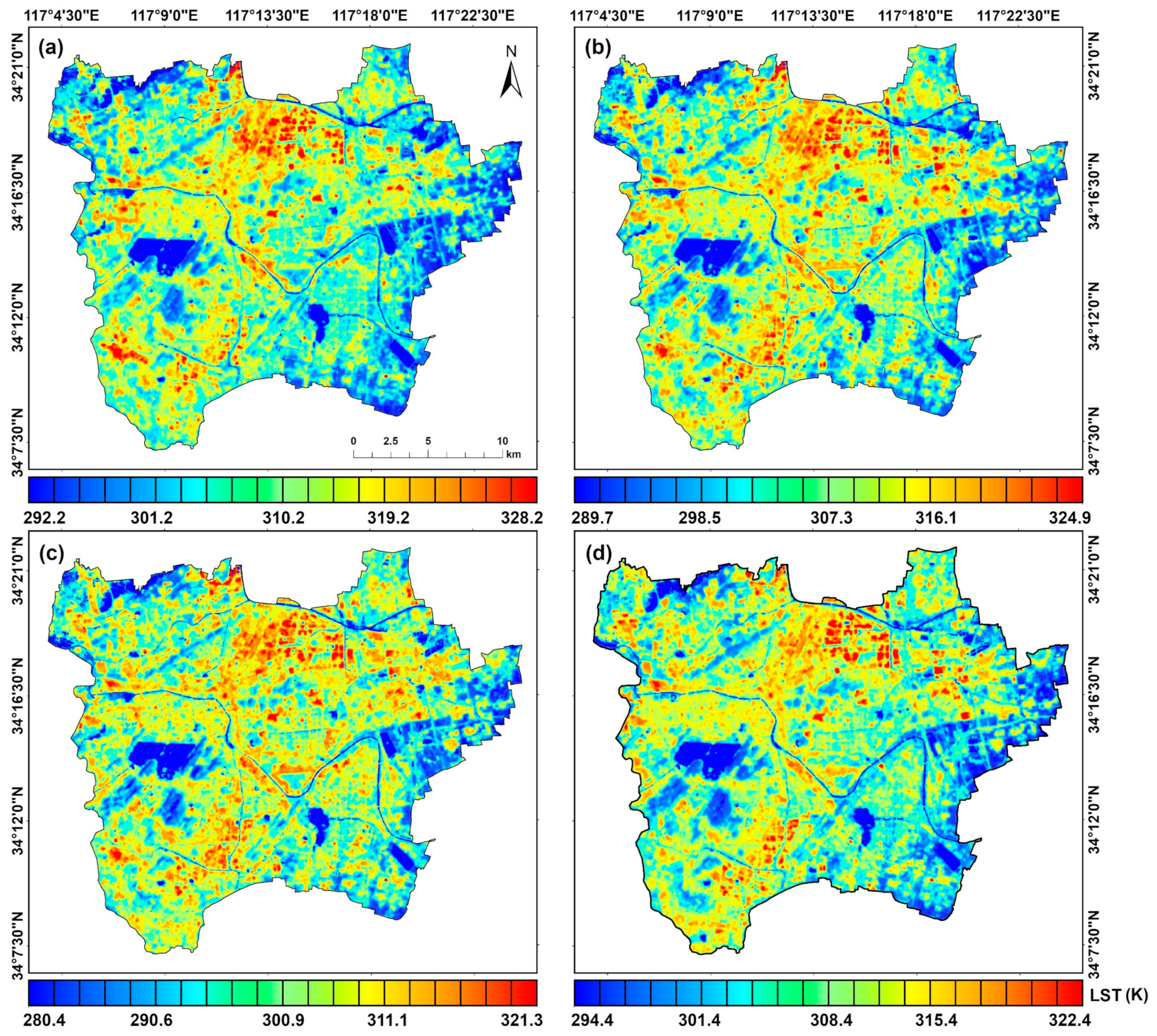
3.1. Inversion Results for VF and LST
3.2. Bivariate Moran’s I between Landscape Metrics of VF-Level Patches and LST
3.3. Impact Weight of Class-Level VFLMs of LV4 and LV5 on LST
4. Discussion
5. Conclusions
Author Contributions
Funding
Data Availability Statement
Acknowledgments
Conflicts of Interest
Appendix A
Appendix B
References
- He, B.-J.; Wang, J.; Zhu, J.; Qi, J. Beating the Urban Heat: Situation, Background, Impacts and the Way Forward in China. Renew. Sustain. Energy Rev. 2022, 161, 112350. [Google Scholar] [CrossRef]
- Santamouris, M. Recent Progress on Urban Overheating and Heat Island Research. Integrated Assessment of the Energy, Environmental, Vulnerability and Health Impact. Synergies with the Global Climate Change. Energy Build. 2020, 207, 109482. [Google Scholar] [CrossRef]
- Rakoto, P.Y.; Deilami, K.; Hurley, J.; Amati, M.; Sun, Q. (Chayn) Revisiting the Cooling Effects of Urban Greening: Planning Implications of Vegetation Types and Spatial Configuration. Urban For. Urban Green. 2021, 64, 127266. [Google Scholar] [CrossRef]
- Amati, M.; Taylor, L. From Green Belts to Green Infrastructure. Plan. Pract. Res. 2010, 25, 143–155. [Google Scholar] [CrossRef]
- Chen, A.; Yao, X.A.; Sun, R.; Chen, L. Effect of Urban Green Patterns on Surface Urban Cool Islands and Its Seasonal Variations. Urban For. Urban Green. 2014, 13, 646–654. [Google Scholar] [CrossRef]
- Shih, W. Greenspace Patterns and the Mitigation of Land Surface Temperature in Taipei Metropolis. Habitat Int. 2017, 60, 69–80. [Google Scholar] [CrossRef]
- Bowler, D.E.; Buyung-Ali, L.; Knight, T.M.; Pullin, A.S. Urban Greening to Cool Towns and Cities: A Systematic Review of the Empirical Evidence. Landsc. Urban Plan. 2010, 97, 147–155. [Google Scholar] [CrossRef]
- Horváthová, E.; Badura, T.; Duchková, H. The Value of the Shading Function of Urban Trees: A Replacement Cost Approach. Urban For. Urban Green. 2021, 62, 127166. [Google Scholar] [CrossRef]
- Colter, K.R.; Middel, A.C.; Martin, C.A. Effects of Natural and Artificial Shade on Human Thermal Comfort in Residential Neighborhood Parks of Phoenix, Arizona, USA. Urban For. Urban Green. 2019, 44, 126429. [Google Scholar] [CrossRef]
- Deilami, K.; Rudner, J.; Butt, A.; MacLeod, T.; Williams, G.; Romeijn, H.; Amati, M. Allowing Users to Benefit from Tree Shading: Using a Smartphone App to Allow Adaptive Route Planning during Extreme Heat. Forests 2020, 11, 998. [Google Scholar] [CrossRef]
- Hsieh, C.M.; Li, J.J.; Zhang, L.; Schwegler, B. Effects of Tree Shading and Transpiration on Building Cooling Energy Use. Energy Build. 2018, 159, 382–397. [Google Scholar] [CrossRef]
- Wang, X.; Dallimer, M.; Scott, C.E.; Shi, W.; Gao, J. Tree Species Richness and Diversity Predicts the Magnitude of Urban Heat Island Mitigation Effects of Greenspaces. Sci. Total Environ. 2021, 770, 145211. [Google Scholar] [CrossRef] [PubMed]
- Lee, P.S.-H.; Park, J. An Effect of Urban Forest on Urban Thermal Environment in Seoul, South Korea, Based on Landsat Imagery Analysis. Forests 2020, 11, 630. [Google Scholar] [CrossRef]
- Zhang, Y.; Chen, L.L.; Wang, Y.; Chen, L.L.; Yao, F.; Wu, P.; Wang, B.; Li, Y.; Zhou, T.; Zhang, T. Research on the Contribution of Urban Land Surface Moisture to the Alleviation Effect of Urban Land Surface Heat Based on Landsat 8 Data. Remote Sens. 2015, 7, 10737–10762. [Google Scholar] [CrossRef]
- Guo, G.; Wu, Z.; Chen, Y. Complex Mechanisms Linking Land Surface Temperature to Greenspace Spatial Patterns: Evidence from Four Southeastern Chinese Cities. Sci. Total Environ. 2019, 674, 77–87. [Google Scholar] [CrossRef]
- Estoque, R.C.; Murayama, Y.; Myint, S.W. Effects of Landscape Composition and Pattern on Land Surface Temperature: An Urban Heat Island Study in the Megacities of Southeast Asia. Sci. Total Environ. 2017, 577, 349–359. [Google Scholar] [CrossRef]
- Zhou, W.; Cao, F. Effects of Changing Spatial Extent on the Relationship between Urban Forest Patterns and Land Surface Temperature. Ecol. Indic. 2020, 109, 105778. [Google Scholar] [CrossRef]
- NOAA’s Satellite and Information Service (NESDIS) NOAA National Centers for Environmental Information. Available online: https://www.ngdc.noaa.gov/ (accessed on 7 September 2022).
- Li, L.; Canters, F.; Solana, C.; Ma, W.; Chen, L.; Kervyn, M. Discriminating Lava Flows of Different Age within Nyamuragira’s Volcanic Field Using Spectral Mixture Analysis. Int. J. Appl. Earth Obs. Geoinf. 2015, 40, 1–10. [Google Scholar] [CrossRef]
- Heinz, D.C.D.C.; Chang, C.I. Fully Constrained Least Squares Linear Spectral Mixture Analysis Method for Material Quantification in Hyperspectral Imagery. IEEE Trans. Geosci. Remote Sens. 2001, 39, 529–545. [Google Scholar] [CrossRef]
- Small, C. Estimation of Urban Vegetation Abundance by Spectral Mixture Analysis. Int. J. Remote Sens. 2001, 22, 1305–1334. [Google Scholar] [CrossRef]
- Wu, C.; Murray, A.T. Estimating Impervious Surface Distribution by Spectral Mixture Analysis. Remote Sens. Environ. 2003, 84, 493–505. [Google Scholar] [CrossRef]
- Ridd, M.K. Exploring a V-I-S (Vegetation-Impervious Surface-Soil) Model for Urban Ecosystem Analysis through Remote Sensing: Comparative Anatomy for Cities. Int. J. Remote Sens. 1995, 16, 2165–2185. [Google Scholar] [CrossRef]
- Wu, C. Normalized Spectral Mixture Analysis for Monitoring Urban Composition Using ETM+ Imagery. Remote Sens. Environ. 2004, 93, 480–492. [Google Scholar] [CrossRef]
- Wu, J. Effects of Changing Scale on Landscape Pattern Analysis: Scaling Relations. Landsc. Ecol. 2004, 19, 125–138. [Google Scholar] [CrossRef]
- Teng, M.; Zeng, L.; Zhou, Z.; Wang, P.; Xiao, W.; Dian, Y. Responses of Landscape Metrics to Altering Grain Size in the Three Gorges Reservoir Landscape in China. Environ. Earth Sci. 2016, 75, 1055. [Google Scholar] [CrossRef]
- Oyana, T.J.; Johnson, S.J.; Wang, G. Landscape Metrics and Change Analysis of a National Wildlife Refuge at Different Spatial Resolutions. Int. J. Remote Sens. 2014, 35, 3109–3134. [Google Scholar] [CrossRef]
- Chefaoui, R.M. Landscape Metrics as Indicators of Coastal Morphology: A Multi-Scale Approach. Ecol. Indic. 2014, 45, 139–147. [Google Scholar] [CrossRef]
- Kong, F.; Nakagoshi, N. Spatial-Temporal Gradient Analysis of Urban Green Spaces in Jinan, China. Landsc. Urban Plan. 2006, 78, 147–164. [Google Scholar] [CrossRef]
- Wu, J.; Shen, W.; Sun, W.; Tueller, P.T. Empirical Patterns of the Effects of Changing Scale on Landscape Metrics. Landsc. Ecol. 2002, 17, 761–782. [Google Scholar] [CrossRef]
- Barsi, J.; Schott, J.; Hook, S.; Raqueno, N.; Markham, B.; Radocinski, R. Landsat-8 Thermal Infrared Sensor (TIRS) Vicarious Radiometric Calibration. Remote Sens. 2014, 6, 11607–11626. [Google Scholar] [CrossRef]
- Montanaro, M.; Lunsford, A.; Tesfaye, Z.; Wenny, B.; Reuter, D. Radiometric Calibration Methodology of the Landsat 8 Thermal Infrared Sensor. Remote Sens. 2014, 6, 8803–8821. [Google Scholar] [CrossRef]
- Wang, F.; Qin, Z.; Song, C.; Tu, L.; Karnieli, A.; Zhao, S. An Improved Mono-Window Algorithm for Land Surface Temperature Retrieval from Landsat 8 Thermal Infrared Sensor Data. Remote Sens. 2015, 7, 4268–4289. [Google Scholar] [CrossRef]
- Qin, Z.; Karnieli, A.; Berliner, P. A Mono-Window Algorithm for Retrieving Land Surface Temperature from Landsat TM Data and Its Application to the Israel-Egypt Border Region. Int. J. Remote Sens. 2001, 22, 3719–3746. [Google Scholar] [CrossRef]
- Zhang, Y.; Li, L.; Chen, L.; Liao, Z.; Wang, Y.; Wang, B.; Yang, X. A Modified Multi-Source Parallel Model for Estimating Urban Surface Evapotranspiration Based on ASTER Thermal Infrared Data. Remote Sens. 2017, 9, 1029. [Google Scholar] [CrossRef]
- Anselin, L. Local Indicators of Spatial Association—LISA. Geogr. Anal. 1995, 27, 93–115. [Google Scholar] [CrossRef]
- Zhang, Y.; Liu, Y.; Zhang, Y.; Liu, Y.; Zhang, G.; Chen, Y. On the Spatial Relationship between Ecosystem Services and Urbanization: A Case Study in Wuhan, China. Sci. Total Environ. 2018, 637–638, 780–790. [Google Scholar] [CrossRef]
- Liu, R.X.; Kuang, J.; Gong, Q.; Hou, X.L. Principal Component Regression Analysis with Spss. Comput. Methods Programs Biomed. 2003, 71, 141–147. [Google Scholar] [CrossRef]
- Dutta, K.; Basu, D.; Agrawal, S. Synergetic Interaction between Spatial Land Cover Dynamics and Expanding Urban Heat Islands. Environ. Monit. Assess. 2021, 193, 184. [Google Scholar] [CrossRef]
- Wetherley, E.B.; McFadden, J.P.; Roberts, D.A. Megacity-Scale Analysis of Urban Vegetation Temperatures. Remote Sens. Environ. 2018, 213, 18–33. [Google Scholar] [CrossRef]
- Zaitunah, A.; Samsuri, S.; Silitonga, A.F.; Syaufina, L. Urban Greening Effect on Land Surface Temperature. Sensors 2022, 22, 4168. [Google Scholar] [CrossRef]
- Zhao, H.; Tan, J.; Ren, Z.; Wang, Z. Spatiotemporal Characteristics of Urban Surface Temperature and Its Relationship with Landscape Metrics and Vegetation Cover in Rapid Urbanization Region. Complexity 2020, 2020, 1–12. [Google Scholar] [CrossRef]

| Satellite | Sensor Resolution | Scene ID | Acquisition Date | Acquisition Time (GMT + 8) |
|---|---|---|---|---|
| Landsat 8 | OLI: 30 m TIRS: 100 m | LC81210362014121LGN00 | 1 May 2014 | 10:42:29 |
| LC81220362017136LGN00 | 16 May 2017 | 10:48:22 | ||
| LC81220362018123LGN00 | 3 May 2018 | 10:48:04 | ||
| LC81210362020138LGN00 | 17 May 2020 | 10:42:10 | ||
| GF-1 | PAN: 2 m MSS: 8 m | GF1_PMS1_E117.2_N34.1_20200428_L1A0004767917 | 28 April 2020 | 11:14:21 |
| GF1_PMS1_E117.3_N34.4_20200428_L1A0004767915 | 28 April 2020 | 11:14:17 |
| Date | Acquisition Time (GMT + 8) | Air Temperature (K) | Air Relative Humidity (%) |
|---|---|---|---|
| 1 May 2014 | 11:00:00 | 297.42 | 55.12 |
| 16 May 2017 | 11:00:00 | 296.33 | 39.76 |
| 3 May 2018 | 11:00:00 | 294.96 | 48.00 |
| 17 May 2020 | 11:00:00 | 299.48 | 53.19 |
| VF Levels | Interval |
|---|---|
| Extreme-high VF (Level 5, LV5) | VF > VF_mean + std |
| Sub-high VF (Level 4, LV4) | VF_mean + 0.5std < VF ≤ VF_mean + std |
| Medium VF (Level 3, LV3) | VF_mean − 0.5std < VF ≤ VF_mean + 0.5std |
| Sub-low VF (Level 2, LV2) | VF_mean − std < VF ≤ VF_mean − 0.5std |
| Extreme-low VF (Level 1, LV1) | VF < VF_mean − std |
| Metrics | Equation | Description | Parameter Explanation | |
|---|---|---|---|---|
| Class level | PLAND | Porportion of the patch type | aij—the area of patch ij; A—total landscape area; eik—total length (m) of edge in landscape between patch types (classes) i and k; gii—number of adjacent patches of the same landscape type i; pij—perimeter of patch ij in terms of number of cell surfaces; Z—total number of cells in the landscape. | |
| LPI | Porportion of the largest patch type | |||
| LSI | Shape complexity degree of the patch type | |||
| AI | Aggregation degree of the patch type | |||
| COHESION | Natural connectivity degree between patches | |||
| Landscape level | SHDI | Diversity indicator of all patch types | pi—proportion of the landscape occupied by patch type (class) i; m—number of patch types (classes) present in the landscape, excluding the landscape border if present; N—number of patches in the landscape of patch type (class) i; A—total landscape area. | |
| SHEI | Even distribution indicator of all patch types | |||
| PD | Number of patches per unit area | |||
| CONTAG | Aggregation degree of all patch types | |||
| w (g·cm−2) | τ Functions | Tair_e Function |
|---|---|---|
| 0.2–1.6 | 0.9184–0.0725w | 16.0110 + 0.9262Tair |
| 1.6–4.4 | 1.0163–0.1330w | |
| 4.4–5.4 | 0.7029–0.0620w |
| Date | KMO | Sums of Squared Loadings | F1 ① | F2 ① |
|---|---|---|---|---|
| 1 May 2014 | 0.7190 | Eigenvalue (λi) | 4.02 | 3.74 |
| Cumulative percent (%) | 77.56 | |||
| 16 May 2017 | 0.7109 | Eigenvalue (λi) | 4.00 | 3.71 |
| Cumulative percent (%) | 77.14 | |||
| 3 May 2018 | 0.7096 | Eigenvalue (λi) | 3.89 | 3.84 |
| Cumulative percent (%) | 77.32 | |||
| 17 May 2020 | 0.6855 | Eigenvalue (λi) | 3.89 | 3.88 |
| Cumulative percent (%) | 77.74 | |||
| Normalized Original Variables (Class-Level VFLMs) | 1 May 2014 | 16 May 2017 | 3 May 2018 | 17 May 2020 | ||||
|---|---|---|---|---|---|---|---|---|
| F1 (θ1) | F2 (θ2) | F1 (θ1) | F2 (θ1) | F1 (θ1) | F2 (θ2) | F1 (θ1) | F2 (θ2) | |
| (X1) PLAND_LV5 | 0.914 | / | 0.910 | / | 0.914 | / | 0.921 | / |
| (X2) COHESION_LV5 | 0.914 | / | 0.911 | / | 0.909 | / | 0.914 | / |
| (X3) LPI_LV5 | 0.883 | / | 0.880 | / | 0.885 | / | 0.891 | / |
| (X4) AI_LV5 | 0.827 | / | 0.838 | / | 0.826 | / | 0.823 | / |
| (X5) LSI_LV5 | 0.627 | 0.572 | 0.611 | 0.586 | 0.596 | 0.579 | / | |
| (X6) PLAND_LV4 | 0.341 | 0.875 | 0.372 | 0.868 | 0.300 | 0.896 | / | 0.908 |
| (X7) COHESION_LV4 | / | 0.923 | / | 0.924 | / | 0.924 | / | 0.935 |
| (X8) LPI_LV4 | / | 0.873 | / | 0.883 | / | 0.880 | / | 0.883 |
| (X9) AI_LV4 | / | 0.733 | / | 0.705 | / | 0.733 | / | 0.724 |
| (X10) LSI_LV4 | 0.555 | 0.632 | 0.531 | 0.624 | 0.513 | 0.631 | 0.519 | 0.642 |
| Regression Coefficients | 1 May 2014 | 16 May 2017 | 3 May 2018 | 17 May 2020 | |
|---|---|---|---|---|---|
| r | 0.569 *** | 0.612 *** | 0.553 *** | 0.644 *** | |
| R2 | 0.323 *** | 0.375 *** | 0.306 *** | 0.415 *** | |
| Regression Constant | 0.949 *** | 0.578 *** | 0.693 *** | 0.635 *** | |
| Unstandardized Coefficients | F1 | −0.010 *** | −0.110 *** | −0.083 *** | −0.109 *** |
| F2 | −0.004 *** | −0.066 *** | −0.014 *** | −0.054 *** | |
| Standardized Coefficients (βi) | β1 | −0.474 *** | −0.463 *** | −0.516 *** | −0.538 *** |
| β2 | −0.139 *** | −0.207 *** | −0.060 *** | −0.179 *** |
Publisher’s Note: MDPI stays neutral with regard to jurisdictional claims in published maps and institutional affiliations. |
© 2022 by the authors. Licensee MDPI, Basel, Switzerland. This article is an open access article distributed under the terms and conditions of the Creative Commons Attribution (CC BY) license (https://creativecommons.org/licenses/by/4.0/).
Share and Cite
Zhang, Y.; Wang, Y.; Ding, N. Spatial Effects of Landscape Patterns of Urban Patches with Different Vegetation Fractions on Urban Thermal Environment. Remote Sens. 2022, 14, 5684. https://doi.org/10.3390/rs14225684
Zhang Y, Wang Y, Ding N. Spatial Effects of Landscape Patterns of Urban Patches with Different Vegetation Fractions on Urban Thermal Environment. Remote Sensing. 2022; 14(22):5684. https://doi.org/10.3390/rs14225684
Chicago/Turabian StyleZhang, Yu, Yuchen Wang, and Nan Ding. 2022. "Spatial Effects of Landscape Patterns of Urban Patches with Different Vegetation Fractions on Urban Thermal Environment" Remote Sensing 14, no. 22: 5684. https://doi.org/10.3390/rs14225684
APA StyleZhang, Y., Wang, Y., & Ding, N. (2022). Spatial Effects of Landscape Patterns of Urban Patches with Different Vegetation Fractions on Urban Thermal Environment. Remote Sensing, 14(22), 5684. https://doi.org/10.3390/rs14225684


