Article

Relationships between Land Surface Temperatures and Neighboring Environment in Highly Urbanized Areas: Seasonal and Scale Effects Analyses of Beijing, China

1
Aerospace Information Research Institute, Chinese Academy of Sciences, Beijing 100094, China
2
University of Chinese Academy of Sciences, Beijing 100049, China
3
Key Laboratory of Earth Observation of Hainan Province, Hainan Aerospace Information Research Institute, Sanya 572029, China
4
Environment & Climate Changes Research Institute, National Water Research Centre, El Qanater EI Khairiya 13621/5, Egypt
5
School of Computing, Ulster University, Shore Rd., Newtownabbey BT37 0QB, UK
6
Alba Regia Technical Faculty, Óbuda University, Budai ut 45., H-8000 Szekesfehervar, Hungary
*
Author to whom correspondence should be addressed.
Remote Sens. 2022, 14(17), 4340; https://doi.org/10.3390/rs14174340
Submission received: 19 July 2022 / Revised: 26 August 2022 / Accepted: 30 August 2022 / Published: 1 September 2022
(This article belongs to the Special Issue Geographical Analysis and Modeling of Urban Heat Island Formation)

Abstract

:
Urban environments have a strong influence on the land surface temperature (LST) in urban areas. Understanding the relationship between LST and urban environmental factors can help develop effective strategies to reduce high LSTs in urban areas, which is critical for mitigating the urban heat island effect. Previous studies have focused on the correlation between LST and the environmental factors that drive its formation, without considering the influences of the neighboring environment and the vertical expansion of highly urbanized areas. Notably, the correlation between LST and its neighboring environment in different seasons remains unclear. In this study, we selected central Beijing in China as our study area and employed the moving window method to characterize the environmental factors of the neighboring environment of the central LST cell. We explored eight environmental factors from three layers: normalized difference vegetation index (NDVI), normalized difference built-up index (NDBI), modified normalized difference water index (MNDWI), building density (BD), building height (BH), building volume (BV), sky view factor (SVF), and road density (RD). The Pearson correlation and extreme gradient boosting (XGB) regression methods were applied to measure the correlation between LST and the different factors in moving windows of different sizes. The results indicated that the correlation between NDVI, MNDWI, and LST was considerably different in the winter and other seasons. However, NDBI was positively correlated with LST in all seasons, although the correlation was strongest/weakest in summer/winter. Among building-related factors, BD and BH were more strongly correlated with LST, and the positive/negative correlation between BD/BH and LST was stronger in summer/winter. The correlation between LST and its neighboring environment varied with increasing window size, and this variation differs significantly between winter and other seasons. In spring, summer, and autumn, the strength of the correlation between LST and its neighboring environment showed an “inverted V” pattern with increasing window size. The optimal spatial scales to explore the influence of neighboring environments on the LST of 30-m cells were 210 m and 270 m. This study revealed the seasonal correlation between LST and its neighboring environment while explaining the variation at a spatial scale. Notably, this study can provide a new perspective for understanding the driving mechanism of the urban thermal environment, while contributing to its scientific optimization and management.

1. Introduction

With the acceleration of urbanization, the development of urban heat islands (UHIs) in cities being warmer than surrounding rural areas has been observed frequently on a global scale [1,2,3]. High urban temperatures not only facilitate energy consumption for cooling [4], contributing to air-pollutant emissions and global warming [5], but also increase the risk of heat-related morbidity and mortality, especially during extreme heat events [6,7,8]. At present, over 50% of the global population lives in urban areas, and this proportion is expected to reach 70% by 2050 [9]. The negative impacts of UHIs pose a great threat to sustainable urban development [2,3]. Land surface temperature (LST), an effective indicator of surface UHI, is generally affected by various factors related to urbanization [10,11]. Disclosing the correlation between LST and urban environmental factors is critical in developing reasonable strategies to optimize the urban thermal environment, prevent the further intensification of the UHI effect, and achieve sustainable development.
Urbanization is a complex process characterized by the transformation of natural land cover types (e.g., vegetation, water bodies, forests, and croplands) to impervious surfaces, such as roads, buildings, pavements, and parking lots [12,13]. Previous studies have confirmed that impervious surfaces can absorb and retain heat, resulting in higher surface temperatures in urban areas [2]. In addition, roads in urban areas are associated with traffic activities that lead to waste heat emissions [10]. Hardened pavement areas and the number of private vehicles are related to road density (RD) [14]. Therefore, urban road networks cannot be excluded when analyzing the potential driving factors of urban surface temperature. Vegetation and water bodies have an important cooling effect that can reduce the LST in urban areas [15]. Widely studied surface biophysical indexes, including the normalized difference built-up index (NDBI) [16], normalized difference vegetation index (NDVI) [17], and modified normalized difference water index (MNDWI) [18], exhibited different correlations with LST. Reducing impervious surface areas and increasing urban green vegetation/water areas are ideal strategies to mitigate high temperatures in urban areas. However, in highly urbanized areas, the amount of space available for greening is limited and it is impractical to considerably reduce impervious surfaces, such as buildings and roads. Meanwhile, studies in 3D urban morphology have indicated that optimizing urban building forms can help mitigate the UHI effect [19,20,21,22,23]. As a result, there is increasing interest regarding the effects of multidimensional factors of urban environments on LST [9,24,25,26].
In highly urbanized areas, buildings reflect urban expansion in the vertical dimension. This has also been the most important urban landscape in 3D urban morphology studies. The combination of high buildings and narrow streets can trap long-wave radiation and increase the degree of thermal stress in summer and solar radiation absorption [27,28]. However, the shadows of high-rise buildings can reduce the absorption of solar radiation by the ground [29]. Thus, a comprehensive investigation of the relationship between LST and building-related factors is crucial for urban planning and intra-urban thermal environment management. Although recent studies examine the relationship between LST and building factors, including building density (BD), building height (BH), building volume (BV), and sky view factor (SVF) factors [19,20,25,30,31], most of them focus on specific seasons, with the summer receiving the most attention. More studies are required to understand the correlations between building factors and LST during different seasons. Moreover, previous studies on the relationship between LST and building features have yielded inconsistent results. A study conducted at the residential scale suggested that building height had a greater impact on LST than building density [19]. However, a seasonal analysis at a geographical scale of 500 m × 500 m indicated that building density had a stronger influence on LST than building height [21]. A recent study based on a road-block scale also indicated that the influence of building cover ratio on LST was stronger than building height [20]. These inconsistent conclusions suggest that the correlations between building factors and LST may be affected by the spatial scale. However, at present, only a few studies have comprehensively discussed the seasonal and scale characteristics of the correlation between building factors and LST [9].
The neighboring environment plays an important role in the driving mechanism of the LST in highly urbanized areas. Previous studies have confirmed that the cooling effects of urban vegetation and water bodies are largely regulated by neighboring vegetation and impervious surface landscapes [32,33]. The heat sources in urban areas, such as industrial parks, contribute to the increase in the surface temperatures within a certain spatial extent around them [34]. Thus, these findings suggest that the local LST is related to the neighboring environment. However, the strength of the correlation between LST and land cover varies with spatial resolution, indicating the spatial range of the effect of the neighboring environment on LST [25,35]. Determining the effect of neighboring environments on LST provides a new perspective for understanding the potential driving factors of the urban thermal environment in a comprehensive manner. Thus, there is an increasing interest in the thermal effects of the neighboring environment. However, in investigating the thermal effects of neighboring environments, previous studies mainly focused on special urban scenarios, such as public and industrial parks and meteorological station areas, without considering the general situation. Therefore, more case studies are required to measure the influence of neighboring environments on fine-scale LSTs in highly urbanized areas.
In this study, we analyzed the central urban area of Beijing; the moving window method was adopted to measure the neighboring environmental factors of LST at different spatial scales. Eight environmental factors were selected from the urban greenness, urban wetness, and urban grayness layers: NDVI, NDBI, MNDWI, BD, BH, BV, SV, and RD. The Pearson correlation and extreme gradient boosting (XGB) regression methods were used to measure the influence of these factors on the LST from the perspectives of individual and combined effects. The aim of this study is to address the following questions: (1) What are the seasonal differences in the correlations between LST and the neighboring environment, in terms of multidimensional factors? (2) How does a change in spatial scale affect the correlation between LST and the neighboring environment? What are the optimal spatial scales? (3) Finally, is there any inter-seasonal difference in the effects of spatial scale on the correlation between LST and its neighboring environment?
This study aims to reveal the seasonal and scale effects on the correlations between LST and multidimensional environmental factors from the perspective of neighboring environments to improve the understanding of the driving mechanism of the urban thermal environment.

2. Study Area and Dataset

2.1. Study Area

Beijing is located on the North China Plain and experiences a continental monsoon climate (hot and rainy in the summer and cold and dry in the winter). As the capital of China, Beijing has undergone rapid urbanization in the last four decades. Its permanent population increased gradually from 10.47 million in 1987 to 21.94 million in 2017 (URL: http://nj.tjj.beijing.gov.cn/nj/main/2021-tjnj/zk/indexch.htm, accessed on 1 June 2022). The percentage of the urban population was 86.45% in 2017. Rapid urbanization has dramatically changed urban landscape patterns and caused a variety of environmental problems, including water and air pollution and the UHI effect. The deterioration of the thermal environment has become a major challenge for sustainable urban development in Beijing. Notably, urbanization in Beijing occurs in a ring-shaped pattern, that is, a concentric expansion from the urban center to the periphery. The region within the Fourth Ring Road covers most of the central urban areas that have the highest urbanization rates and population densities and contains various land cover types and complicated landscape patterns. Therefore, in this study, we investigated the thermal environment of the region within the Fourth Ring Road of Beijing, which covers an area of 340.26 km², and covers all of the Core Functional Zone and a small part of the Urban Function Extended Zone (Figure 1).

2.2. Dataset

The dataset used in this study included Landsat-8 Operational Land Imager/Thermal Infrared Sensor (OLI/TIRS) images and building and road network data. The Landsat-8 OLI/TIRS images obtained from the Geospatial Data Cloud official website (http://www.gscloud.cn/, accessed on 28 November 2020) were used to estimate the LST and surface biophysical factors. After screening all of the available images for 2017, four Landsat-8 OLI/TIRS images collected on May 23 (spring), July 10 (summer), September 28 (autumn), and December 17 (winter) were employed to characterize the thermal environment for different seasons [36]. The building data used to acquire building-related factors were obtained from the Baidu, Inc. (https://map.baidu.com, accessed on 1 October 2017) with a spatial resolution of 10 m. The building data can describe the geographical location and height attributes of buildings in 2017 and cover the area within the Fourth Ring Road of Beijing. The road data in 2017 were obtained from the OpenStreetMap (http://www.openstreetmap.org, accessed on 1 June 2020), a substantial global spatial database, and were used to explore the thermal effects of road density on the LST in this study.

3. Methods

3.1. Land Surface Temperature (LST) Estimation

In this study, the radiative transfer equation (RTE) method was employed to estimate the LST from the Landsat-8 OLI/TIRS images. The RTE method is more accurate than the split window method and single channel method and could guarantee an accuracy of 0.6 K for the retrieved LST [37,38]. First, the RTE method was used to estimate the black-body radiation brightness by removing the influence of the atmosphere. This can be expressed in an equation, as follows:
B T S = L λ L τ 1 ε L / L λ ε
where B T S is the black-body radiation; L λ (W/m2·sr·μm) is the spectral radiation brightness for band 10; τ is the transmittance of thermal infrared bands in the atmosphere; L (W/m2·sr·μm) and L (W/m2·sr·μm) indicate the upwelling and downwelling atmospheric radiance (http://atmcorr.gsfc.nasa.gov, accessed on 28 November 2020), respectively; and ε denotes the land surface emissivity, which is calculated based on vegetation proportion [38]. Finally, according to the Plank function, the LST was derived from B T S , using the following equation:
T s = K 2 / ln K 1 / B T S + 1 273
where T s is the LST (°C), K 2 is 1321.08 K, and K 1 is 774.89 (W/m2·sr·μm).
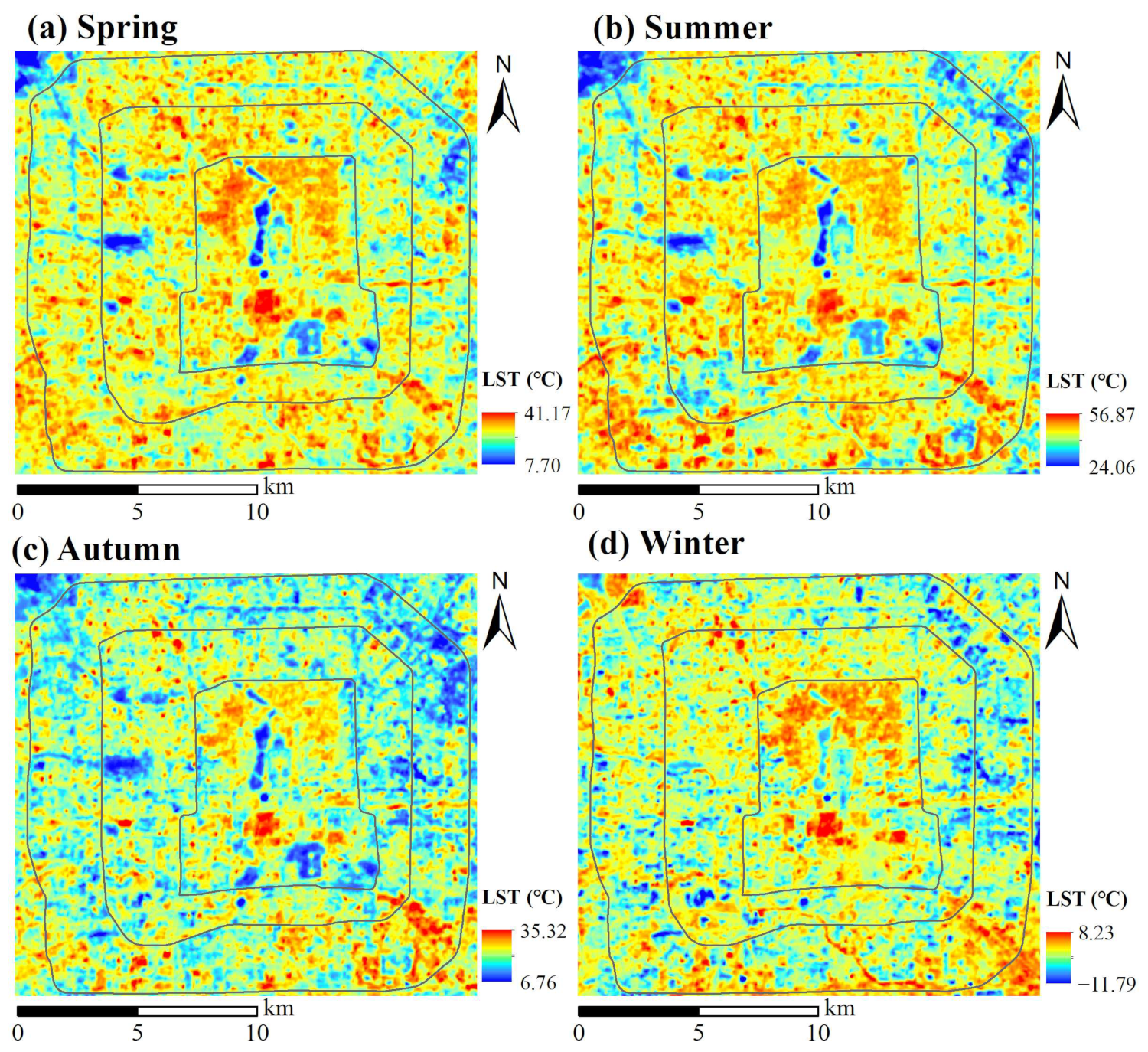
The spatial distribution of the LST in spring, summer, autumn, and winter is shown in Figure 2. The high-temperature area is significant for understanding the spatiotemporal pattern of LST and optimizing the thermal environment. We observed three seasonal stable high-temperature areas in the study area, mainly distributed within the Second Ring Road. Compared with the high-temperature areas inside the Second Ring Road, the distribution of the high-temperature areas located outside the road was relatively fragmented.

3.2. Selection and Calculation of Multidimensional Environmental Factors

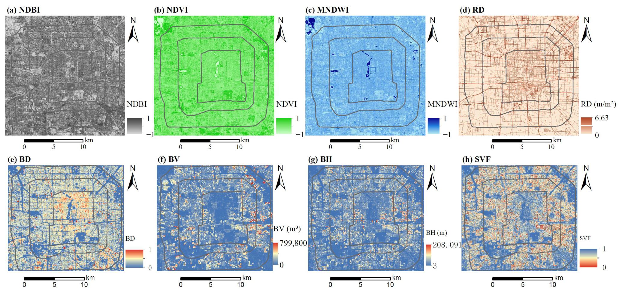
The LST in urban areas is mainly determined by complex urban landscapes. According to previous studies, the driving factors of LST can be categorized into three layers: urban greenness, wetness, and grayness (Table 1). In this study, three surface biophysical factors (NDVI, NDBI, and MNDWI) were selected to represent the overall spatial distributions of urban greenness, grayness, and wetness, respectively, from a two-dimensional (2D) perspective. Buildings and roads are two typical artificial construction types in urban areas, as well as the main components of urban grayness. In this study, we employed RD, BD, BH, BV, and SVF to describe the detailed spatial characteristics of the urban grayness components from 2D and 3D perspectives. The BD was defined as the proportion of the ground building area per unit of analysis, and RD was defined as the total length of the roads in an analysis unit divided by the area of the unit. The BH was defined as the average height of the buildings per unit of analysis, and BV was defined as the total building volume per unit of analysis. Furthermore, S V F j was defined as the proportion of visible sky at a certain observation point j and was calculated based on the buildings, according to the method proposed by [39]. Then, all the S V F j values per analysis unit were averaged. Since seasonal effects were considered in this study, the three surface biophysical factors chosen in this study were calculated separately from four Landsat-8 images captured during the different seasons, whereas the building and road-related factors were considered to be the same for all seasons. The spatial distributions of the selected environmental factors are shown in Figure 3.

3.3. Moving Window Samples for Analysis

The moving window method is a common multiscale analysis approach [43]. The method can be used to capture the continuous spatial variation in specific characteristics of the urban environment at custom scales [44]. In this study, for each analysis sample, the dependent variable was the LST value of the central cell of the moving window, and each independent variable was the average value of the corresponding environmental factor within the moving window. To investigate the influence of the spatial scale, 20 window sizes were used to characterize the urban environmental factors and measure their relationship with the LST of 30-m cells. Since the spatial resolution of the LST data in this study is 30 m, the minimum window size is 90 m × 90 m, which can ensure a clear central pixel in the window. Moreover, the growth interval of the window size is twice the spatial resolution of the LST data, which helps to capture the spatially continuous neighboring environmental characteristics. In addition, a sufficient range of moving window size is necessary to adequately explore the correlation between LST and multiple environmental factors, especially to explore how the correlation changes with increasing window size. Therefore, in this study, the window size was increased from 90 m × 90 m to 1230 m × 1230 m, with an interval of 60 m. The samples obtained from the moving windows of different sizes were used in the subsequent analysis to reveal the response of the LST to its neighboring environment.

3.4. Correlations between Land Surface Temperature (LST) and Environmental Factors

In this study, the Pearson correlation method [45,46], which has been widely used in previous studies, was used to measure the correlation direction and intensity between LST and the selected environmental factors. Twenty correlation coefficients were estimated for each factor in each season, corresponding to twenty sizes of the moving windows. One of the aims of this study was to investigate the seasonal variations in the effects of the urban environment on LST. Therefore, the mean values of the correlation coefficients were calculated for the individual factors with respect to different seasons. In each season, three environmental factors were identified as the dominant driving factors of LST, according to the correlation intensity. Then, the spatial characteristics of the effects of the dominant driving factors on LST were explored by analyzing the trend of correlation intensity with increasing window size. Notably, we focused on the effects of dominant driving factors, as they exhibited relatively strong correlations with LST.

3.5. Application of Regression Model to Analyze Correlation between Land Surface Temperature (LST) and Environmental Factors

Regression models are an efficient method for measuring the combined effects of multiple driving factors on LST. The XGB regression model was used in this study according to its advantages and our research needs. In this study, we aimed to explore the variation in combined effects of multiple environmental factors on LST with increasing window size in different seasons. Compared with statistical linear regression models, the XGB regression model, a tree machine learning regression method, is better adapted to the complex nonlinear relationships between LST and its driving factors. In addition, the XGB regression model is not affected by multicollinearity among driving factors, which means that all environmental factors can be entered into the model [47]. At present, XGB regression is the most effective stochastic gradient boosting algorithm. The idea of the XGB regression model is to build a series of shallow regression trees using a gradient boosting technique, where each tree attempts to correct the residuals in the predictions made by previous trees [48]. The XGB regression model can calculate the optimal solution for the whole model and reduce the overfitting phenomenon [49]. Notably, previous study has confirmed that the XGB regression model outperforms random forest, support vector, and decision tree regressions with higher accuracy in LST prediction [50]. Moreover, the XGB regression model has shown good application effects in many fields, including crime prediction [47], vegetation mapping [51], algal biochar yield prediction [52], flood susceptibility modeling [53], and urban thermal environment [54]. Therefore, in this study, we developed XGB regression models to measure the combined effects of multiple environmental factors on LST. The samples were randomly partitioned into 80% and 20% for training and validation, respectively. The performance of the regression model was measured using the coefficient of determination (R²) metric, which indicated the goodness of fit. It also represented the proportion of variance of the LST, explained by the independent variables in the model. In addition, the root mean square error (RMSE) and the mean absolute error (MAE) were used to evaluate the accuracy of the regression model. The measured R², RMSE, and MAE were calculated using the following equations:
R 2 y , y ^ = 1 i = 1 n y i y i ^ 2 i = 1 n y i y ¯ 2
y ¯ = 1 n i = 1 n y i
R M S E y , y ^ = 1 n   i = 1 n y i y i ^ 2  
M A E y , y ^ = 1 n   i = 1 n y i y i ^
where y i ^ is the predictive value of the i-th sample, and y i is the corresponding true value for n samples.

4. Results

4.1. Seasonal Correlations between Land Surface Temperature (LST) and Neighboring Environmental Factors

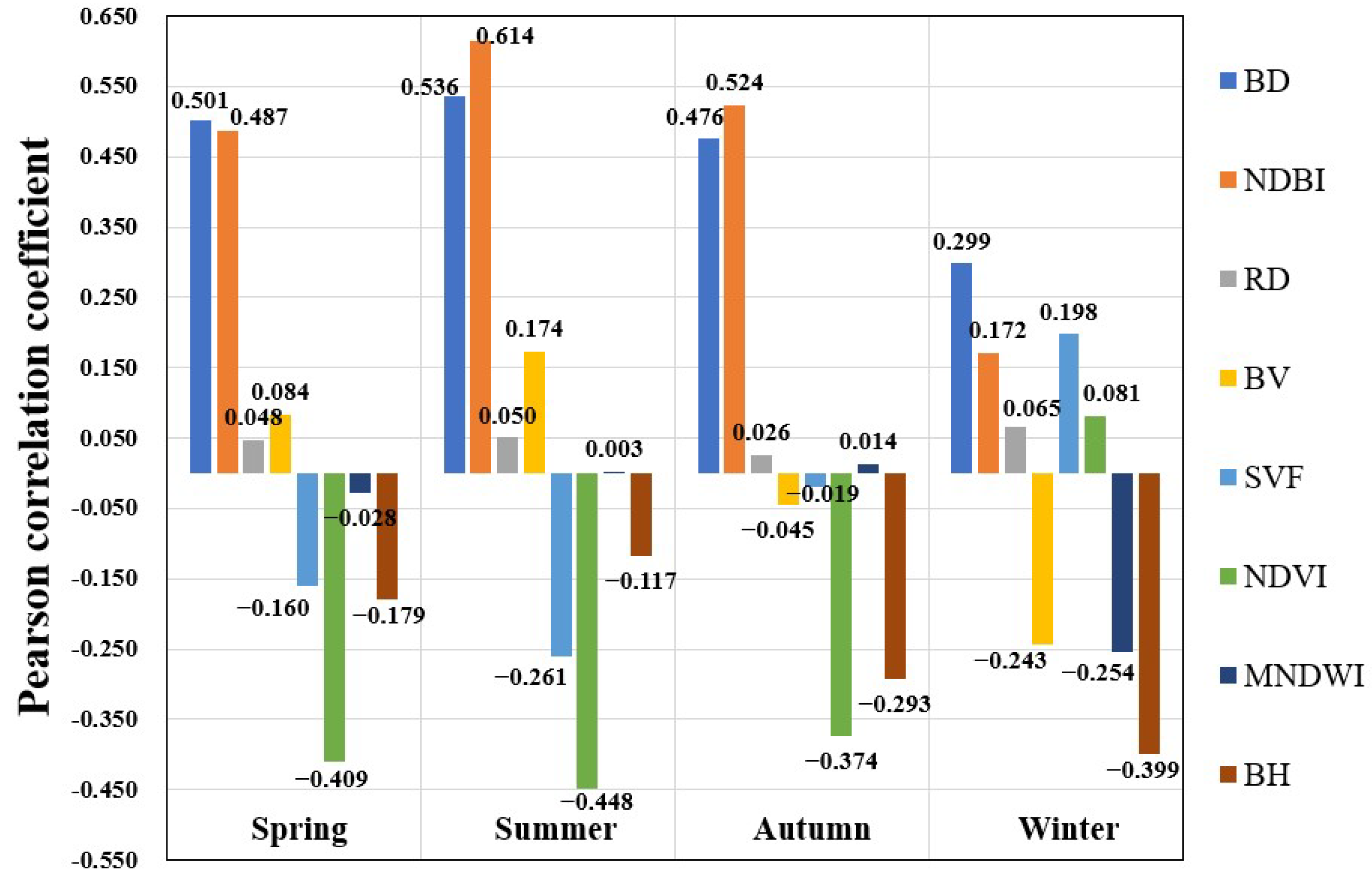
The average correlation between the LST and environmental factors with respect to different seasons is shown in Figure 4. The Pearson correlation coefficient indicated the direction and intensity of the correlation between the LST and environmental factors. The average correlation results were at the 95% significance level. In terms of the direction of correlation, all factors, except BV, SVF, and NDVI, exhibited consistent correlations with the LST in Beijing across all seasons. In addition, the correlation strengths between the urban environmental factors and LST were strong in summer and weak in winter, in terms of the strongest correlation factors.
We observed positive correlations between the BD, NDBI, and RD and the LST in all of the seasons. The correlation between BD and LST was strong (0.501, 0.536, 0.476, and 0.299 in four seasons, respectively), whereas that between RD and LST was weak (0.048, 0.050, 0.026, and 0.065 in four seasons, respectively). These results indicated that the positive association between LST and building density was stronger, whereas the influence of urban road networks on LST was limited. The NDBI factor represented the overall grayness features of the urban area, including both building and road features; therefore, its correlation with LST was similar to that of the BD factor. Notably, the positive correlations between the NDBI and BD factors and the LST of the city were consistent in the spring (0.487), summer (0.614), and autumn (0.524) seasons; their correlation strengths with LST were stronger in spring, summer, and autumn than in winter. This indicated that the warming effect of urban grayness factors was more prominent during warm seasons. Furthermore, BH was negatively correlated with the LST in all seasons, which was completely different from the BD factor, although the latter also represented building characteristics. This result indicated that BD increased the LST of the area, and conversely, BH decreased the LST. In addition, the results also showed that the strength of the correlation between the BH and LST of the city was highest in winter (−0.399). The correlation of the MNDWI factor with the LST was weak and almost negligible in spring, summer, and autumn, with its negative correlation with LST being evident in winter (−0.254).
The direction of the correlation between the urban environmental factors and LST was also reversed during seasonal changes. The BV factor was positively correlated with the LST in the spring (0.084) and summer (0.174) seasons, less correlated with the LST in autumn (−0.045), and negatively correlated with it in winter (−0.243). The changes in the correlations of the SVF and NDVI factors with the LST were similar. Specifically, they both showed negative correlations with the LST in spring (−0.160 and −0.490) and summer (−0.261 and −0.448); the negative correlations weakened in autumn. The factors exhibited positive correlations with the LST in winter (0.198 and 0.081).
In general, there were no significant differences in the correlation results for spring, summer, and autumn. In contrast, the direction or strength of the correlation between each environmental factor and LST changed markedly in winter, compared to that in the other three seasons. These findings imply that the main environmental factors affecting LST in spring, summer, and autumn were consistent to some extent, whereas the factors affecting LST in winter differed from those in warmer seasons.

4.2. Spatial Characteristics of the Correlations between Land Surface Temperature (LST) and Dominant Driving Factors

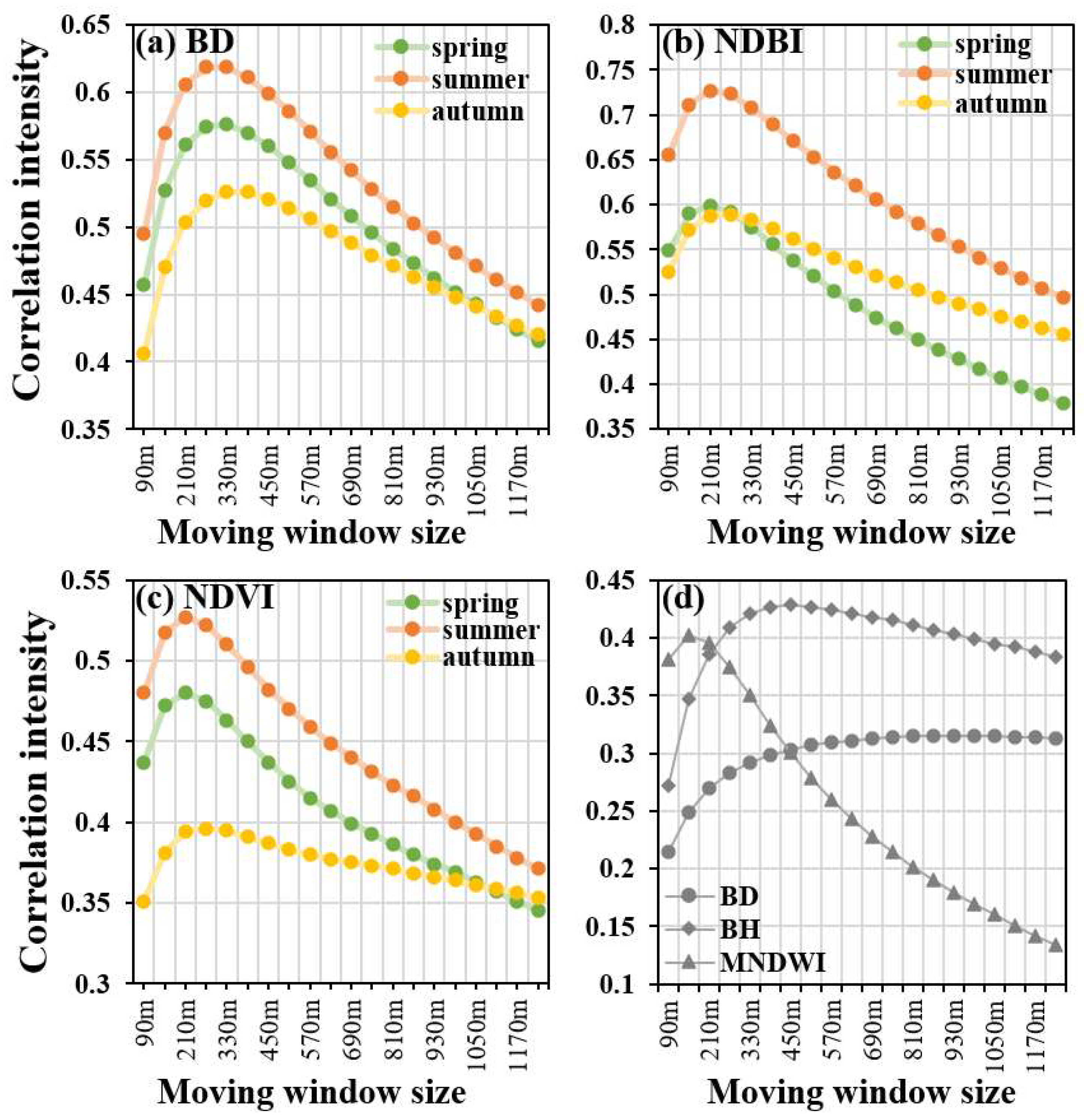
We selected three factors for spring, summer, and autumn (BD, NDBI, and NDVI) and winter (BD, BH, and MNDWI) for further analysis, according to their strong correlations with the LST (Figure 4). This exploration was conducted with various window sizes, i.e., from 90 m to 1230 m, with an interval of 60 m, to reveal the effect of scale through the change in the correlation strength. The influence of the BD, NDBI, and NDVI factors on the LST showed a similar trend, i.e., an inverted V shape with increasing window sizes in relatively warmer seasons (spring, summer, and autumn) (Figure 5a–c). First, the correlation intensity increased with the moving window size and then decreased gradually, which indicated the optimal spatial scales to study the influence of the neighboring environments on the LST. For the BD factor, the intensity of its positive correlation with LST showed an initial sharp rise, followed by a gradual decline after reaching the peak; the peak correlation intensity was obtained when the window size was set at 270 m (summer) and 330 m (spring and autumn). The intensity curve of the NDVI factor associated with LST showed a trend similar to the intensity curve of the BD–LST correlation. The spring curve was located between the summer and autumn curves, and the maximum correlation intensity corresponded to a window size of 210 m (spring and summer) and 270 m (autumn), although the NDVI was negatively correlated with the LST. Similar to the results of BD and NDVI, the summer curve of the NDBI was also at the top, indicating that these environmental factors were most associated with the LST in summer. The difference between the first two was that the gap between the spring and autumn curves gradually increased with the size of the moving window. However, the strongest correlations between the NDBI and LST still occurred at window sizes of 210 m (spring and summer) and 270 m (autumn). The general and intuitive correlations between the environmental factors and LST are shown in Figure 4. The comparative analysis between the scales further revealed that the scales of 210–270 m were more effective in capturing the spatial characteristics of these correlations, regardless of whether the factors were positively (NDBI and BD) or negatively (NDVI) correlated with the LST.
In winter, the BH and MNDWI were negatively correlated with the LST. The curves of these two factors also portrayed an inverted V shape. For example, the correlation intensity between BH and LST first increased sharply, followed by a gradual decrease. The size of the optimal scale at which the strongest correlation strength appeared was 450 m, but the correlation strength at the optimal scale did not differ markedly from that observed for the window size of 1230 m. The correlation intensity curve of the MNDWI also had an inverted V shape, but it differed from that of BH, portraying a sharp decrease with increasing window size. The apex of the curve (corresponding to the strongest correlation) was located at a window size of 150 m. The curve of BD, which was positively correlated to the LST, behaved differently; it continued to rise and then remained flat, without a clear inflection point. The influence of the building characteristics (BH and BD) on the LST was more prominent in the winter. In general, the trend of the winter curve was markedly different from that of the warmer seasons, implying that there was a significant difference in the formation mechanism of the urban thermal environment between the warm (spring, summer, and autumn) and winter seasons.

4.3. Combined Effect of Environmental Factors on Land Surface Temperature (LST)

The LST is the result of the combined effects of multiple factors. Therefore, in this study, the XGB regression method was adopted to construct the LST regression models for different spatial scales in order to investigate the combined effects of these factors on the LST of the city. The explanatory rate indicator, i.e., the percentage of LST variance explained by the regression model, was used to measure the combined effects of these factors on the LST [48]. Figure 6 shows that the RMSE and MAE metrics are lower than 1.6 and 1.2, respectively. Table 2 summarizes the explanatory rates at different scales. For each season, the same color scheme was used to portray the change in the explanatory rate with scale. Green indicates a low explanatory rate and yellow indicates a high explanatory rate. For the spring and summer LST, the XGB regression models established at 210 m had the highest explanatory rate (74.94% and 77.55%, respectively), followed by the model established at 270 m (74.62% and 77.34%, respectively). For the autumn LST, the model established at 270 m had the highest explanatory rate (68.04%), followed by that established at 210 m (67.53%). These results indicated that, when studying the LST during the warm season, the multiple regression model had the strongest interpretation of the LST at a spatial scale of 210–270 m.
Similar to the findings in Section 4.2, the explanatory rate of the XGB regression model and its variation differed markedly between the winter and the warm seasons (spring, summer, and autumn). For the winter LST, the explanatory rate of the model first increased until 57.13% (270 m) and then decreased gradually until 53.10% (570 m); the rate increased again until 60.23% (1230 m). The XGB regression model, including the eight environmental factors, explained the LSTs in spring, summer, and autumn more effectively than that in winter, both in terms of the mean and peak values. These findings suggested that the influencing factors, formation mechanism, and scale effect of the thermal environment in winter were more complex than those observed in the spring, summer, and autumn seasons.

5. Discussion

5.1. Seasonal Characteristics of the Thermal Effects of Urban Environmental Factors

5.1.1. Cooling Effects of Urban Green Vegetation and Water Bodies

Urban vegetation and water bodies are the two main landscape types that provide cooling effects in urban areas and have attracted much attention for improving the urban thermal environment. However, the difference in the cooling effect between the seasons cannot be ignored. In general, urban vegetation decreases the LST through evapotranspiration and shading. The cooling effect of evaporation and shading greatly varies among species and depends on the canopy density in the region [55,56]. It has been confirmed that the cooling effect of tree-cover vegetation is better than that of grass-cover vegetation [57,58]. The results of this study indicated significant inter-seasonal differences in the thermal effects of vegetation and water bodies. The NDVI exhibited a significant negative correlation with the LST in the spring, summer, and autumn seasons, which is consistent with the findings of [59,60]. However, the NDVI exhibited a weak positive correlation with the LST in winter (Figure 4). This finding was consistent with that of a study conducted in North America [61]. Notably, deciduous broad-leaved trees occupy the largest area in Beijing [30]. Additionally, there is an inevitable reduction in green vegetation in winter, resulting in the weakening of the evapotranspiration and shading processes [62]. In addition, the distribution pattern and area of the vegetation may also affect its cooling effect. Therefore, in winter, it is difficult for highly fragmented vegetation to generate a significant cooling effect [19].
Previous studies have indicated that urban water bodies are negatively correlated with LST [63,64]. However, in this study, we observed that the MNDWI factor, an effective indicator of water bodies in urban areas, was weakly correlated to the LST in the spring, summer, and autumn seasons (Figure 4). This discrepancy may be because the total water area in the city is small; therefore, the water body may not be able to provide an effective cooling effect [10]. The MNDWI exhibited a relatively stronger negative correlation with the LST in winter, compared to the NDVI (Figure 4). This finding was consistent with a previous study that reported that the cooling effect of water was stronger than that of vegetation in November [65].

5.1.2. Thermal Effects of Urban Grayness Factors

Buildings, roads, and other impervious surfaces absorb solar radiation, resulting in higher temperatures in urban areas [21,66,67,68]. In this study, the NDBI, BD, and RD were positively correlated to the LST in all the seasons. The strength of the correlation between RD and LST indicated the limited impact of RD on LST, which was consistent with the findings of [41]. A recent study showed that the correlation between the NDBI and LST was weaker in winter than in other seasons [69]. Similarly, in this study, the NDBI and BD exhibited stronger correlations with the LST in summer than that in winter (Figure 4 and Figure 5). Buildings in urban areas are typically closely related to a variety of human activities. For example, in summer, buildings with air conditioning release large amounts of heat, contributing to an increase in the LST [70]. Similarly, the cold air emitted from the air conditioner during winter can reduce the LST. Therefore, the seasonal characteristics of the effects of the NDBI and BD on the LST may be influenced by the amount of solar radiation absorbed by the impervious surface areas and the heat/cooling emissions from buildings. Although the positive correlations of BD and NDBI with the LST have been widely reported, our study revealed seasonal variations in the strength of their correlations with the LST in urban areas at fine scales.
In this study, the BV, an indicator of the total volume of buildings, was positively/negatively correlated to LST in summer/winter. The larger values of BV indicate the higher intensity of the anthropogenic activity and possible larger amount of anthropogenic heat emissions, which is expected to increase LST [71]. In addition, in winter, there may be a larger amount of cooling emissions from buildings in the region with larger BV. A previous study conducted in Berlin and Cologne also observed the positive correlation between BV and LST in summer [42], however, the correlation between BV and LST in winter was positive. This difference could be explained by the different climate backgrounds of urban areas. The influence of SVF on LST is complicated and conflicting conclusions on the correlation between LST and SVF have been reported in previous studies [72,73,74]. Larger SVF indicated more effective air circulation and heat dissipation, and it also means that there may be more incoming solar radiation. Smaller SVF hinders airflow movement and is not conducive to heat dissipation, and it also means the possibility of a larger area of shadow. In our study, the correlation between SVF and LST was season-varying. Similarly, a study conducted in Wuhan city also found a season-varying correlation between SVF and LST [9]. Notably, in this study, the SVF was negatively correlated to LST in summer, which is consistent with a recent study conducted in Beijing [72]. In addition, the negative/positive correlation between SVF and LST in summer/winter may be associated to the anthropic activities, as the smaller SVF is not conducive to the dissipation of the heat/cooling emissions from buildings in summer/winter.
In particular, BH was negatively correlated with the LST in all seasons, which was in line with the results of previous studies [9,19,20]. This may be because the shadows provided by high-rise buildings prevented the nearby ground from absorbing solar radiation, thus, reducing the LST [20,29]. Therefore, higher buildings are expected to formulate lower temperatures owing to their possible larger shadows [20]. Additionally, the negative effect of BH on LST was stronger in winter and autumn than in other seasons, which can also be explained by the larger shadow area in the winter and autumn seasons due to the lower solar elevation [9]. The results related to building features can provide reliable references for the planning and construction of urban buildings. In addition to urban vegetation and water body planning, the season-stable negative effect of BH on LST could provide new insights for the mitigation of the UHI effect for effective urban building planning.

5.2. Spatial Characteristic of the Thermal Effects of Neighboring Environment

Previous studies have confirmed that the cooling effects of urban vegetation and water bodies are largely regulated by the vegetation and impervious surface landscapes of the neighboring regions [32,33]. The heat sources in urban areas, such as industrial parks, will continue to contribute to the increase in the LST within a certain spatial extent around them [34]. These findings indicate that the neighboring environment plays an important role in the driving mechanism of LSTs in urban areas. In addition, the correlations between LST and surface coverage indicators generally vary with the geographical scale [66,75]. This may be related to the diversity of the surface cover features at different geographic scales [62]. Therefore, an appropriate spatial scale is vital for the quantitative analysis of the influence of the neighboring environment on the LST, balancing useful surrounding environment information with the irrelevant information of the distant surrounding environment. Notably, LST is the result of a combination of driving factors, which implies that it is necessary to consider the individual and combined effects of various factors. Therefore, we used both the correlation analysis and the XGB regression method to measure the correlation between the urban environmental factors and LST at different spatial scales.
In this study, the correlation between the urban environmental factors and LST portrayed an initial increasing trend with increasing spatial scales, followed by a decreasing trend (Figure 5 and Table 2), which implied the spatial range of the influence of the neighboring environment on the LST of the 30-m cell. The strongest correlation between the NDVI and LST was obtained within a 210-m moving window size in spring and summer and a 270-m size in autumn (Figure 5). This finding is in line with that of [25], in which the vegetation cover exhibited the highest correlation with the LST within a 210-m moving window in summer. Another study conducted in India also indicated that the median cooling range of urban green spaces was approximately 270 m outside the boundary [76]. The correlations between the MNDWI and LST in winter varied with the sizes of the moving windows and peaked at 150 m (Figure 5). This finding was consistent with the findings of [32], which concluded that the cooling range of water bodies was approximately 74 m. A previous study conducted in the Phoenix metropolitan area indicated that the correlation between impervious surfaces and maximum air temperature in the warm season decreased after a 210-m spatial scale, and the strongest negative correlation between vegetation cover and maximum air temperature occurred at 210 m and 270 m spatial scales [35]. In this study, the optimal spatial scale for exploring the correlation relationship between the 30-m LST and its neighboring environment was 210–270 m in warm seasons (spring, summer, and autumn), considering the individual and combined correlations between the LST and multidimensional factors of the urban environment (Figure 5 and Table 2). These findings suggest that 210–270 m could be an appropriate spatial scale for characterizing the relationship between the LST and its neighboring environment in Beijing. These findings could provide a reference for spatial-scale selection in future LST studies in Beijing and other large cities in northern China.

5.3. Limitations and Scope for Future Work

This study established a viable framework to explore the influence of neighboring environments on LST, considering the multidimensional features of dominant urban landscape types. However, this study has a few limitations. First, although we considered the seasonal variation in the LST, using only one daytime scene collected in each season to obtain LST and surface biophysical indices could be insufficient. In addition, the acquisition time of the images should be considered to ensure that the images can accurately reflect the characteristics of LST in different seasons. Adopting multiple daytime and nighttime images from different seasons to address this aspect may prove to be more efficient in future studies. Second, this study was conducted only in the urban areas of Beijing, and more cities in different climate zones should be considered in future studies [30]. Third, this study explored the thermal effects of buildings and roads. However, the spatial resolution of LST was coarser than that of the building data in the study area. LST data with higher spatial resolution are expected to reveal more accurate relationships between LST and urban 3D landscapes. Moreover, the positional accuracy of roads data from the OpenStreetMap is mainly determined by the positioning technologies and references used by volunteers while digitizing these data [77]. The roads data with high positioning accuracy and accurate information on the width attributes should be considered in future works, although the accuracy of OSM road network data (+/− 20 m) is better than that of other publicly available global datasets such as Global Roads Open Access Data Set (+/− 500 m) [78]. In addition, more factors such as building types/patterns, tree species/patterns, and anthropogenic heat [79], are worthy of future study. Fourth, this study focused on the combined effect of multiple factors on LST in the regression analysis, and the contribution of each environmental factor is worth exploring in future studies. Finally, the thermal effects of urban environmental factors and their spatial scale characteristics differed markedly between seasons, mainly between winter and the warmer seasons. Further studies are required to explain the different driving mechanisms of the thermal environment in winter and other seasons.

6. Conclusions

In recent years, rapid urbanization has caused a series of significant changes in green vegetation, impervious surfaces, human activities, energy consumption, and thermal emissions, and the UHI effect has become increasingly severe. This study was conducted in the central urban areas of Beijing and investigated how the LST of 30-m cells correlated with their neighboring environment in different seasons. Moving windows were applied to characterize the environmental factors of neighboring environments, with a total of 20 spatial scales ranging from 90–1230 m. Eight environmental factors were explored from three layers of urban greenness, wetness, and grayness: NDVI, MNDWI, NDBI, BD, BH, BV, SVF, and RD. The Pearson correlation and XGB regression methods were used to measure the correlation between these factors and the LST, while considering the individual and combined effect.
This study confirmed the significant seasonal differences in the correlation between the LST of 30-m cells and their neighboring environments. The correlation between the NDVI and MNDWI and the LST was considerably different between the winter and the other seasons, indicating that the cooling effects of urban vegetation and water bodies were associated with the season. The NDBI, as a comprehensive indicator of urban grayness, was positively correlated to the LST in all four seasons, indicating that the increasing impervious surfaces can promote an increase in the LST. Reasonable control of the growth of impervious surfaces can help prevent further deterioration of the UHI effect. Road density had a limited impact on LST, whereas buildings had a significant impact on LST. Notably, BD and BH were more strongly correlated to LST than other building factors. BD was positively correlated with LST in all four seasons, indicating that the increasing building density promoted higher LST. BD and NDBI were more strongly correlated with LST in summer than in winter, implying that anthropogenic heat production due to seasonal changes may also affect the correlation between urban grayness and LST. Owing to the shadow effect, high BH values contributed to low LSTs in urban areas. Notably, there was a negative correlation between LST and BH in all four seasons, and this negative correlation was stronger in winter than in summer. In addition to increasing urban green space, the building density and height characteristics can be optimized to help mitigate the UHI effect.
The correlation between LST and its neighboring environment varied with spatial scale, with inter-seasonal differences in the scale effect, mainly between winter and other seasons. In spring, summer, and autumn, the strength of correlation between LST and its neighboring environment portrayed an “inverted V” pattern with increasing spatial scale in terms of the Pearson correlation and XGB regression results, indicating the spatial range of the strongest influence of the neighboring environment on LST of 30-m cells, i.e., the optimal spatial scale to explore the relationship between LST and its neighboring environment. Considering the correlation of individual factors with LST and the explanatory rate of the XGB regression model for LST, 210 m and 270 m were considered as the optimal scales to explore the relationship between LST and its neighboring environment in this study, which can provide a reference for the selection of spatial scales in quantitative LST driving force studies.
These findings contribute to the understanding of the correlation between LST and multidimensional environmental factors in urban areas from the perspective of the neighboring environment. Additionally, the framework developed in this study can be applied to other urban areas. The results of these studies can help urban planners develop rational strategies for optimizing urban thermal environments.

Author Contributions

Conceptualization, W.L. and Q.M.; methodology, W.L. and J.G.; software and writing—original draft, W.L.; data curation, W.L. and Q.M.; writing—review, Q.M., L.Z., M.A., Y.B., X.H., T.J. and D.H.; writing—review and editing, W.L., M.A. and Q.M.; visualization, W.L.; supervision, Q.M.; funding acquisition, Q.M. All authors have read and agreed to the published version of the manuscript.

Funding

This research was funded by the National Natural Science Foundation of China Major Program, grant number 42192580, 42192584; the National Natural Science Foundation of China, grant number 42171357; the National Key Research and Development Program, grant number 2020YFC0833100; and the Bilateral Chinese-Hungarian Project, grant numbers 2019-2.1.11-TÉT-2020-00171.

Data Availability Statement

The data presented in this study are available on request from the corresponding website.

Conflicts of Interest

The authors declare no conflict of interest. The funders had no role in the design of the study; in the collection, analyses, or interpretation of data; in the writing of the manuscript, or in the decision to publish the results.

References

  1. Oke, T.R. The energetic basis of the urban heat island. Q. J. R. Meteorol. Soc. 1982, 108, 1–24. [Google Scholar] [CrossRef]
  2. Ziter, C.D.; Pedersen, E.J.; Kucharik, C.J.; Turner, M.G. Scale-dependent interactions between tree canopy cover and impervious surfaces reduce daytime urban heat during summer. Proc. Natl. Acad. Sci. USA 2019, 116, 7575–7580. [Google Scholar] [CrossRef]
  3. Mora, C.; Dousset, B.; Caldwell, I.R.; Powell, F.E.; Geronimo, R.C.; Bielecki, C.R.; Counsell, C.W.; Dietrich, B.S.; Johnston, E.T.; Louis, L.V. Global risk of deadly heat. Nat. Clim. Chang. 2017, 7, 501–506. [Google Scholar] [CrossRef]
  4. Frayssinet, L.; Merlier, L.; Kuznik, F.; Hubert, J.-L.; Milliez, M.; Roux, J.-J. Modeling the heating and cooling energy demand of urban buildings at city scale. Renew. Sustain. Energy Rev. 2018, 81, 2318–2327. [Google Scholar] [CrossRef]
  5. Akbari, H.; Kurn, D.M.; Bretz, S.E.; Hanford, J.W. Peak power and cooling energy savings of shade trees. Energy Build. 1997, 25, 139–148. [Google Scholar] [CrossRef]
  6. Taylor, J.; Wilkinson, P.; Davies, M.; Armstrong, B.; Chalabi, Z.; Mavrogianni, A.; Symonds, P.; Oikonomou, E.; Bohnenstengel, S.I. Mapping the effects of urban heat island, housing, and age on excess heat-related mortality in London. Urban Clim. 2015, 14, 517–528. [Google Scholar] [CrossRef]
  7. Anderson, G.B.; Bell, M.L. Heat waves in the United States: Mortality risk during heat waves and effect modification by heat wave characteristics in 43 US communities. Environ. Health Perspect. 2011, 119, 210–218. [Google Scholar] [CrossRef]
  8. Jenerette, G.D.; Harlan, S.L.; Buyantuev, A.; Stefanov, W.L.; Declet-Barreto, J.; Ruddell, B.L.; Myint, S.W.; Kaplan, S.; Li, X. Micro-scale urban surface temperatures are related to land-cover features and residential heat related health impacts in Phoenix, AZ USA. Landsc. Ecol. 2016, 31, 745–760. [Google Scholar] [CrossRef]
  9. Li, H.; Li, Y.; Wang, T.; Wang, Z.; Gao, M.; Shen, H. Quantifying 3D building form effects on urban land surface temperature and modeling seasonal correlation patterns. Build. Environ. 2021, 204, 108132. [Google Scholar] [CrossRef]
  10. Peng, J.; Jia, J.; Liu, Y.; Li, H.; Wu, J. Seasonal contrast of the dominant factors for spatial distribution of land surface temperature in urban areas. Remote Sens. Environ. 2018, 215, 255–267. [Google Scholar] [CrossRef]
  11. Do Nascimento, A.C.L.; Galvani, E.; Gobo, J.P.A.; Wollmann, C.A. Comparison between air temperature and land surface temperature for the city of São Paulo, Brazil. Atmosphere 2022, 13, 491. [Google Scholar] [CrossRef]
  12. Chen, J.; Zhan, W.; Jin, S.; Han, W.; Du, P.; Xia, J.; Lai, J.; Li, J.; Liu, Z.; Li, L. Separate and combined impacts of building and tree on urban thermal environment from two-and three-dimensional perspectives. Build. Environ. 2021, 194, 107650. [Google Scholar] [CrossRef]
  13. Wollmann, C.A.; Hoppe, I.L.; Gobo, J.P.A.; Simioni, J.P.D.; Costa, I.T.; Baratto, J.; Shooshtarian, S. Thermo-hygrometric variability on waterfronts in negative radiation balance: A case study of balneário Camboriú/SC, Brazil. Atmosphere 2021, 12, 1453. [Google Scholar] [CrossRef]
  14. Hu, X.; Wu, Z.; Wu, C.; Ye, L.; Lan, C.; Tang, K.; Xu, L.; Qiu, R. Effects of road network on diversiform forest cover changes in the highest coverage region in China: An analysis of sampling strategies. Sci. Total Environ. 2016, 565, 28–39. [Google Scholar] [CrossRef]
  15. Gunawardena, K.R.; Wells, M.J.; Kershaw, T. Utilising green and bluespace to mitigate urban heat island intensity. Sci. Total Environ. 2017, 584, 1040–1055. [Google Scholar] [CrossRef]
  16. Guha, S.; Govil, H.; Dey, A.; Gill, N. Analytical study of land surface temperature with NDVI and NDBI using Landsat 8 OLI and TIRS data in Florence and Naples city, Italy. Eur. J. Remote Sens. 2018, 51, 667–678. [Google Scholar] [CrossRef]
  17. Alexander, C. Normalised difference spectral indices and urban land cover as indicators of land surface temperature (LST). Int. J. Appl. Earth Obs. Geoinf. 2020, 86, 102013. [Google Scholar] [CrossRef]
  18. Xu, H. Modification of normalised difference water index (NDWI) to enhance open water features in remotely sensed imagery. Int. J. Remote Sens. 2006, 27, 3025–3033. [Google Scholar] [CrossRef]
  19. Zheng, Z.; Zhou, W.; Yan, J.; Qian, Y.; Wang, J.; Li, W. The higher, the cooler? Effects of building height on land surface temperatures in residential areas of Beijing. Phys. Chem. Earth Parts A/B/C 2019, 110, 149–156. [Google Scholar] [CrossRef]
  20. Sun, F.; Liu, M.; Wang, Y.; Wang, H.; Che, Y. The effects of 3D architectural patterns on the urban surface temperature at a neighborhood scale: Relative contributions and marginal effects. J. Clean. Prod. 2020, 258, 120706. [Google Scholar] [CrossRef]
  21. Guo, G.; Zhou, X.; Wu, Z.; Xiao, R.; Chen, Y. Characterizing the impact of urban morphology heterogeneity on land surface temperature in Guangzhou, China. Environ. Model. Softw. 2016, 84, 427–439. [Google Scholar] [CrossRef]
  22. Das, M.; Das, A. Assessing the relationship between local climatic zones (LCZs) and land surface temperature (LST)—A case study of Sriniketan-Santiniketan Planning Area (SSPA), West Bengal, India. Urban Clim. 2020, 32, 100591. [Google Scholar] [CrossRef]
  23. Du, P.; Chen, J.; Bai, X.; Han, W. Understanding the seasonal variations of land surface temperature in Nanjing urban area based on local climate zone. Urban Clim. 2020, 33, 100657. [Google Scholar] [CrossRef]
  24. Alavipanah, S.; Schreyer, J.; Haase, D.; Lakes, T.; Qureshi, S. The effect of multi-dimensional indicators on urban thermal conditions. J. Clean. Prod. 2018, 177, 115–123. [Google Scholar] [CrossRef]
  25. Alexander, C. Influence of the proportion, height and proximity of vegetation and buildings on urban land surface temperature. Int. J. Appl. Earth Obs. Geoinf. 2021, 95, 102265. [Google Scholar] [CrossRef]
  26. Hu, Y.; Dai, Z.; Guldmann, J.-M. Modeling the impact of 2D/3D urban indicators on the urban heat island over different seasons: A boosted regression tree approach. J. Environ. Manag. 2020, 266, 110424. [Google Scholar] [CrossRef]
  27. Oke, T.R. Canyon geometry and the nocturnal urban heat island: Comparison of scale model and field observations. J. Climatol. 1981, 1, 237–254. [Google Scholar] [CrossRef]
  28. Oke, T.R. Street design and urban canopy layer climate. Energy Build. 1988, 11, 103–113. [Google Scholar] [CrossRef]
  29. Nichol, J.E. High-resolution surface temperature patterns related to urban morphology in a tropical city: A satellite-based study. J. Appl. Meteorol. Climatol. 1996, 35, 135–146. [Google Scholar] [CrossRef]
  30. Song, J.; Chen, W.; Zhang, J.; Huang, K.; Hou, B.; Prishchepov, A.V. Effects of building density on land surface temperature in China: Spatial patterns and determinants. Landsc. Urban Plan. 2020, 198, 103794. [Google Scholar] [CrossRef]
  31. Wu, Z.; Yao, L.; Zhuang, M.; Ren, Y. Detecting factors controlling spatial patterns in urban land surface temperatures: A case study of Beijing. Sustain. Cities Soc. 2020, 63, 102454. [Google Scholar] [CrossRef]
  32. Du, H.; Song, X.; Jiang, H.; Kan, Z.; Wang, Z.; Cai, Y. Research on the cooling island effects of water body: A case study of Shanghai, China. Ecol. Indic. 2016, 67, 31–38. [Google Scholar] [CrossRef]
  33. Qiu, K.; Jia, B. The roles of landscape both inside the park and the surroundings in park cooling effect. Sustain. Cities Soc. 2020, 52, 101864. [Google Scholar] [CrossRef]
  34. Meng, Q.; Hu, D.; Zhang, Y.; Chen, X.; Zhang, L.; Wang, Z. Do industrial parks generate intra-heat island effects in cities? New evidence, quantitative methods, and contributing factors from a spatiotemporal analysis of top steel plants in China. Environ. Pollut. 2022, 292, 118383. [Google Scholar] [CrossRef]
  35. Myint, S.W.; Brazel, A.; Okin, G.; Buyantuyev, A. Combined effects of impervious surface and vegetation cover on air temperature variations in a rapidly expanding desert city. GIScience Remote Sens. 2010, 47, 301–320. [Google Scholar] [CrossRef]
  36. Fu, X.; Yao, L.; Xu, W.; Wang, Y.; Sun, S. Exploring the multitemporal surface urban heat island effect and its driving relation in the Beijing-Tianjin-Hebei urban agglomeration. Appl. Geogr. 2022, 144, 102714. [Google Scholar] [CrossRef]
  37. Yu, X.; Guo, X.; Wu, Z. Land surface temperature retrieval from Landsat 8 TIRS—Comparison between radiative transfer equation-based method, split window algorithm and single channel method. Remote Sens. 2014, 6, 9829–9852. [Google Scholar] [CrossRef]
  38. Sobrino, J.A.; Jiménez-Muñoz, J.C.; Paolini, L.J.R.S.O.E. Land surface temperature retrieval from LANDSAT TM 5. Remote Sens. Environ. 2004, 90, 434–440. [Google Scholar] [CrossRef]
  39. Zakšek, K.; Oštir, K.; Kokalj, Ž.J.R.S. Sky-view factor as a relief visualization technique. Remote Sens. 2011, 3, 398–415. [Google Scholar] [CrossRef]
  40. Weng, Q.; Lu, D.; Schubring, J. Estimation of land surface temperature–vegetation abundance relationship for urban heat island studies. Remote Sens. Environ. 2004, 89, 467–483. [Google Scholar] [CrossRef]
  41. Taripanah, F.; Ranjbar, A. Quantitative analysis of spatial distribution of land surface temperature (LST) in relation Ecohydrological, terrain and socio-economic factors based on Landsat data in mountainous area. Adv. Space Res. 2021, 68, 3622–3640. [Google Scholar] [CrossRef]
  42. Berger, C.; Rosentreter, J.; Voltersen, M.; Baumgart, C.; Schmullius, C.; Hese, S. Spatio-temporal analysis of the relationship between 2D/3D urban site characteristics and land surface temperature. Remote Sens. Environ. 2017, 193, 225–243. [Google Scholar] [CrossRef]
  43. Hagen-Zanker, A. A computational framework for generalized moving windows and its application to landscape pattern analysis. Int. J. Appl. Earth Obs. Geoinf. 2016, 44, 205–216. [Google Scholar] [CrossRef]
  44. Wang, X.; Meng, Q.; Zhang, L.; Hu, D. Evaluation of urban green space in terms of thermal environmental benefits using geographical detector analysis. Int. J. Appl. Earth Obs. Geoinf. 2021, 105, 102610. [Google Scholar] [CrossRef]
  45. Guo, F.; Wu, Q.; Schlink, U. 3D building configuration as the driver of diurnal and nocturnal land surface temperatures: Application in Beijing’s old city. Build. Environ. 2021, 206, 108354. [Google Scholar] [CrossRef]
  46. Peng, J.; Xie, P.; Liu, Y.; Ma, J. Urban thermal environment dynamics and associated landscape pattern factors: A case study in the Beijing metropolitan region. Remote Sens. Environ. 2016, 173, 145–155. [Google Scholar] [CrossRef]
  47. Zhang, X.; Liu, L.; Lan, M.; Song, G.; Xiao, L.; Chen, J. Interpretable machine learning models for crime prediction. Comput. Environ. Urban Syst. 2022, 94, 101789. [Google Scholar] [CrossRef]
  48. Yu, S.; Chen, Z.; Yu, B.; Wang, L.; Wu, B.; Wu, J.; Zhao, F. Exploring the relationship between 2D/3D landscape pattern and land surface temperature based on explainable eXtreme Gradient Boosting tree: A case study of Shanghai, China. Sci. Total Environ. 2020, 725, 138229. [Google Scholar] [CrossRef]
  49. Mousa, S.R.; Bakhit, P.R.; Osman, O.A.; Ishak, S. A comparative analysis of tree-based ensemble methods for detecting imminent lane change maneuvers in connected vehicle environments. Transp. Res. Rec. 2018, 2672, 268–279. [Google Scholar] [CrossRef]
  50. Mohammad, P.; Goswami, A.; Chauhan, S.; Nayak, S. Machine learning algorithm based prediction of land use land cover and land surface temperature changes to characterize the surface urban heat island phenomena over Ahmedabad city, India. Urban Clim. 2022, 42, 101116. [Google Scholar] [CrossRef]
  51. Zhang, H.; Eziz, A.; Xiao, J.; Tao, S.; Wang, S.; Tang, Z.; Zhu, J.; Fang, J. High-resolution vegetation mapping using eXtreme gradient boosting based on extensive features. Remote Sens. 2019, 11, 1505. [Google Scholar] [CrossRef]
  52. Pathy, A.; Meher, S.; Balasubramanian, P. Predicting algal biochar yield using eXtreme Gradient Boosting (XGB) algorithm of machine learning methods. Algal Res. 2020, 50, 102006. [Google Scholar] [CrossRef]
  53. Linh, N.T.T.; Pandey, M.; Janizadeh, S.; Bhunia, G.S.; Norouzi, A.; Ali, S.; Pham, Q.B.; Anh, D.T.; Ahmadi, K. Flood susceptibility modeling based on new hybrid intelligence model: Optimization of XGboost model using GA metaheuristic algorithm. Adv. Space Res. 2022, 69, 3301–3318. [Google Scholar] [CrossRef]
  54. Sun, Y.; Gao, C.; Li, J.; Wang, R.; Liu, J. Evaluating urban heat island intensity and its associated determinants of towns and cities continuum in the Yangtze River Delta Urban Agglomerations. Sustain. Cities Soc. 2019, 50, 101659. [Google Scholar] [CrossRef]
  55. Shahidan, M.F.; Jones, P.J.; Gwilliam, J.; Salleh, E. An evaluation of outdoor and building environment cooling achieved through combination modification of trees with ground materials. Build. Environ. 2012, 58, 245–257. [Google Scholar] [CrossRef]
  56. Rahman, M.A.; Armson, D.; Ennos, A. A comparison of the growth and cooling effectiveness of five commonly planted urban tree species. Urban Ecosyst. 2015, 18, 371–389. [Google Scholar] [CrossRef]
  57. Yang, G.; Yu, Z.; Jørgensen, G.; Vejre, H. How can urban blue-green space be planned for climate adaption in high-latitude cities? A seasonal perspective. Sustain. Cities Soc. 2020, 53, 101932. [Google Scholar] [CrossRef]
  58. Yu, Z.; Yao, Y.; Yang, G.; Wang, X.; Vejre, H. Strong contribution of rapid urbanization and urban agglomeration development to regional thermal environment dynamics and evolution. For. Ecol. Manag. 2019, 446, 214–225. [Google Scholar] [CrossRef]
  59. Chen, L.; Li, M.; Huang, F.; Xu, S. Relationships of LST to NDBI and NDVI in Wuhan City based on Landsat ETM+ image. In Proceedings of the 2013 6th International Congress on Image and Signal Processing (CISP), Hangzhou, China, 16–18 December 2013; pp. 840–845. [Google Scholar]
  60. Mukherjee, S.; Joshi, P.; Garg, R.D. Evaluation of LST downscaling algorithms on seasonal thermal data in humid subtropical regions of India. Int. J. Remote Sens. 2015, 36, 2503–2523. [Google Scholar] [CrossRef]
  61. Sun, D.; Kafatos, M. Note on the NDVI-LST relationship and the use of temperature-related drought indices over North America. Geophys. Res. Lett. 2007, 34. [Google Scholar] [CrossRef] [Green Version]
  62. Zhou, W.; Cao, F. Effects of changing spatial extent on the relationship between urban forest patterns and land surface temperature. Ecol. Indic. 2020, 109, 105778. [Google Scholar] [CrossRef]
  63. Deilami, K.; Kamruzzaman, M.; Liu, Y. Urban heat island effect: A systematic review of spatio-temporal factors, data, methods, and mitigation measures. Int. J. Appl. Earth Obs. Geoinf. 2018, 67, 30–42. [Google Scholar] [CrossRef]
  64. Dai, Z.; Guldmann, J.-M.; Hu, Y. Spatial regression models of park and land-use impacts on the urban heat island in central Beijing. Sci. Total Environ. 2018, 626, 1136–1147. [Google Scholar] [CrossRef] [PubMed]
  65. Yu, Z.W.; Guo, Q.; Sun, R. Impacts of urban cooling effect based on landscape scale: A review. J. Appl. Ecol. 2015, 26, 636–642. [Google Scholar]
  66. Guo, J.; Han, G.; Xie, Y.; Cai, Z.; Zhao, Y. Exploring the relationships between urban spatial form factors and land surface temperature in mountainous area: A case study in Chongqing city, China. Sustain. Cities Soc. 2020, 61, 102286. [Google Scholar] [CrossRef]
  67. Weng, Q.; Rajasekar, U.; Hu, X. Modeling urban heat islands and their relationship with impervious surface and vegetation abundance by using ASTER images. IEEE Trans. Geosci. Remote Sens. 2011, 49, 4080–4089. [Google Scholar] [CrossRef]
  68. Morabito, M.; Crisci, A.; Guerri, G.; Messeri, A.; Congedo, L.; Munafò, M. Surface urban heat islands in Italian metropolitan cities: Tree cover and impervious surface influences. Sci. Total Environ. 2021, 751, 142334. [Google Scholar] [CrossRef]
  69. Guha, S.; Govil, H.; Taloor, A.K.; Gill, N.; Dey, A. Land surface temperature and spectral indices: A seasonal study of Raipur City. Geod. Geodyn. 2022, 13, 72–82. [Google Scholar] [CrossRef]
  70. Hwang, R.-L.; Lin, T.-P.; Lin, F.-Y. Evaluation and mapping of building overheating risk and air conditioning use due to the urban heat island effect. J. Build. Eng. 2020, 32, 101726. [Google Scholar] [CrossRef]
  71. Qian, J.; Meng, Q.; Zhang, L.; Hu, D.; Hu, X.; Liu, W. Improved anthropogenic heat flux model for fine spatiotemporal information in Southeast China. Environ. Pollut. 2022, 299, 118917. [Google Scholar] [CrossRef]
  72. Gu, Y.; You, X.-Y. A spatial quantile regression model for driving mechanism of urban heat island by considering the spatial dependence and heterogeneity: An example of Beijing, China. Sustain. Cities Soc. 2022, 79, 103692. [Google Scholar] [CrossRef]
  73. Yang, X.; Li, Y. The impact of building density and building height heterogeneity on average urban albedo and street surface temperature. Build. Environ. 2015, 90, 146–156. [Google Scholar] [CrossRef]
  74. Scarano, M.; Mancini, F. Assessing the relationship between sky view factor and land surface temperature to the spatial resolution. Int. J. Remote Sens. 2017, 38, 6910–6929. [Google Scholar] [CrossRef]
  75. Guo, L.; Liu, R.; Men, C.; Wang, Q.; Miao, Y.; Zhang, Y. Quantifying and simulating landscape composition and pattern impacts on land surface temperature: A decadal study of the rapidly urbanizing city of Beijing, China. Sci. Total Environ. 2019, 654, 430–440. [Google Scholar] [CrossRef]
  76. Shah, A.; Garg, A.; Mishra, V. Quantifying the local cooling effects of urban green spaces: Evidence from Bengaluru, India. Landsc. Urban Plan. 2021, 209, 104043. [Google Scholar] [CrossRef]
  77. Haklay, M. How good is volunteered geographical information? A comparative study of OpenStreetMap and Ordnance Survey datasets. Environ. Plan. B Plan. Des. 2010, 37, 682–703. [Google Scholar] [CrossRef]
  78. Gong, P.; Chen, B.; Li, X.; Liu, H.; Wang, J.; Bai, Y.; Chen, J.; Chen, X.; Fang, L.; Feng, S.; et al. Mapping Essential Urban Land Use Categories in China (EULUC-China): Preliminary Results for 2018; Lanzhou University: Lanzhou, China, 2020; Volume 65, pp. 182–187. [Google Scholar]
  79. Liu, W.; Meng, Q.; Allam, M.; Zhang, L.; Hu, D.; Menenti, M. Driving factors of land surface temperature in urban agglomerations: A case study in the Pearl River Delta, China. Remote Sens. 2021, 13, 2858. [Google Scholar] [CrossRef]
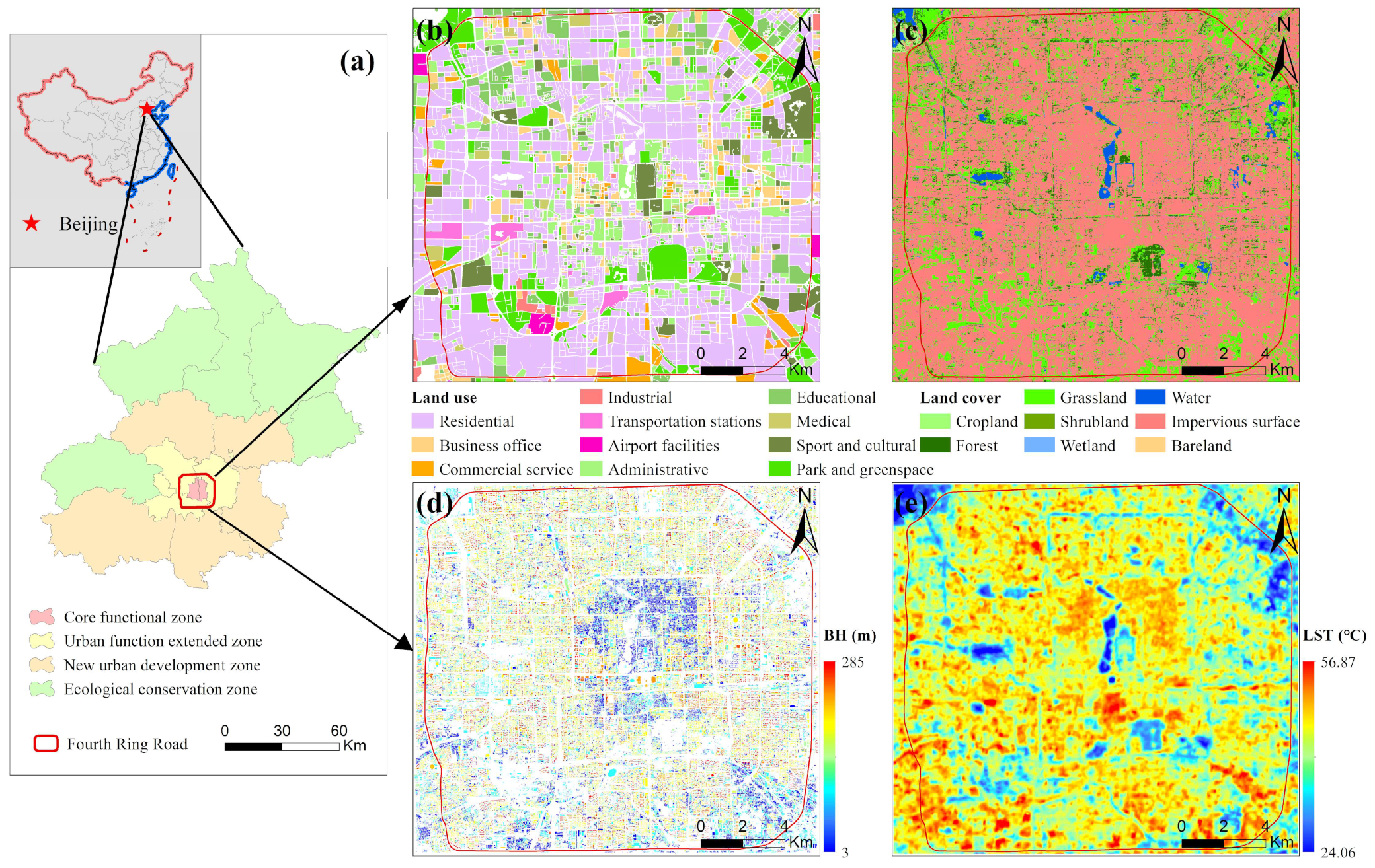
Figure 1. Geographic location of the study area: (a) the location of the Fourth Ring Road of Beijing; (b) the land use map of study area; (c) the land cover map of study area; (d) building height map of study area; (e) the land surface temperature (summer) distribution map of study area (the land use data in 2018 and land cover data in 2017 were derived from the website: http://data.ess.tsinghua.edu.cn/, accessed on 21 August 2022).
Remotesensing 14 04340 g001
Figure 2. Spatial distribution of land surface temperature (LST) in: (a) spring, (b) summer, (c) autumn, and (d) winter.
Remotesensing 14 04340 g002
Figure 3. Spatial distribution of environmental factors considered in this study using different indexes: normalized difference built-up index (NDBI), normalized difference vegetation index (NDVI), modified normalized difference water index (MNDWI), building density (BD), building height (BH), building volume (BV), sky view factor (SVF), and road density (RD). Images for NDBI, NDVI, and MNDWI factors were captured in summer.
Remotesensing 14 04340 g003
Figure 4. Pearson correlations between land surface temperature (LST) and different environmental factors, normalized difference built-up index (NDBI), normalized difference vegetation index (NDVI), modified normalized difference water index (MNDWI), building density (BD), building height (BH), building volume (BV), sky view factor (SVF), and road density (RD).
Remotesensing 14 04340 g004
Figure 5. Correlation intensities of dominant factors: (a) correlation intensities of building density (BD) in spring, summer, and autumn; (b) correlation intensities of normalized difference built-up index (NDBI) in spring, summer, and autumn; (c) correlation intensities of normalized difference vegetation index (NDVI) in spring, summer, and autumn; (d) correlation intensities of BD, building height (BH); and modified normalized difference water index (MNDWI) in winter.
Remotesensing 14 04340 g005
Figure 6. The root mean square error (RMSE) (a) and mean absolute error (MAE) results (b).
Remotesensing 14 04340 g006
Table 1. Description of environmental factors considered in this study.
TypeLayersFactors (Abbreviation)EquationReferenceUnit
Surface biophysical factorsUrban greennessNormalized difference vegetation index (NDVI) NDVI = ρ N I R ρ R e d ρ N I R + ρ R e d [40]-
Urban graynessNormalized difference built-up index (NDBI) NDBI = ρ S W I R 1 ρ N I R ρ S W I R 1 + ρ N I R [16]-
Urban wetnessModified normalized difference water index (MNDWI) MNDWI = ρ G r e e n ρ S W I R 1 ρ G r e e n + ρ S W I R 1 [18]-
Multidimensional factors of two typical components of urban graynessUrban grayness (Road network)Road density (RD) RD = L e n r o a d s Unit area [41]m/m²
Urban grayness (Buildings)Building density (BD) BD = i = 1 n B i a r e a Unit area [30]-
Building height (BH) BH = i = 1 n B i h e i g h t n [42]m
Building volume (BV) BV = i = 1 n B i v o l u m e [42]
Sky view factor (SVF) SVF = i = 1 k S V F j / k [9]-
Note: B i a r e a is the land coverage area of the i-th building in the analysis unit, B i h e i g h t is the height of building i , B i v o l u m e is the volume of building i , n is the total number of buildings in the analysis unit, L e n r o a d s is the total length of all roads in an analysis unit, Unit area is the area of the analysis unit, SVF j is the SVF value of cell j in the analysis unit, and k is the total number of cells in the analysis unit. ρ G r e e n , ρ R e d , ρ N I R , and ρ S W I R 1 represents the band 3, band 4, band 5, and band 6 of Landsat-8, respectively.
Table 2. Percentage of explained variance of the land surface temperature (LST) for different seasons.
Scales (m)Percentage of Explained Variance of LST (%)
SpringSummerAutumnWinter
9064.2966.9456.5246.09
15072.1174.6464.2054.49
21074.9477.5567.5357.12
27074.6277.3468.0457.13
33072.9875.5966.9255.84
39070.7473.3465.5654.48
45068.8671.2364.0753.92
51067.1769.4763.0553.43
57065.9868.1862.0953.10
63065.2767.5961.5253.30
69065.0667.2261.5354.31
75065.0567.0961.7955.20
81064.8866.9361.5955.92
87064.8866.6261.9456.54
93065.2966.3662.2157.14
99065.6966.7562.4257.52
105066.0566.6062.8757.92
111066.1366.6663.3358.52
117066.1566.9463.5359.69
123066.4467.2663.9160.23
Average67.6369.5163.2355.59
Publisher’s Note: MDPI stays neutral with regard to jurisdictional claims in published maps and institutional affiliations.