Supervised Classifications of Optical Water Types in Spanish Inland Waters

Abstract

Remote sensing of lake water quality assumes there is no universal method or algorithm that can be applied in a general way on all inland waters, which usually have different in-water components affecting their optical properties. Depending on the place and time of year, the lake dynamics, and the particular components of the water, non-tailor-designed algorithms can lead to large errors or lags in the quantification of the water quality parameters, such as the suspended mineral sediments, dissolved organic matter, and chlorophyll-a concentration. Selecting the most suitable algorithm for each type of water is not a simple matter. One way to make selecting the most suitable water quality algorithm easier on each occasion is by knowing ahead of time the type of water being handled. This approach is used, for instance, in the Lake Water Quality production chain of the Copernicus Global Land Service. The objective of this work is to determine which supervised classification approach might give the most accurate results. We use a dataset of manually labeled pixels on lakes and reservoirs in Eastern Spain. High-resolution images from the Multispectral Instrument sensor on board the ESA Sentinel-2 satellite, atmospherically corrected with the Case 2 Regional Coast Colour algorithm, are used as the basis for extracting the pixels for the dataset. Three families of different supervised classifiers have been implemented and compared: the K-nearest neighbor, decision trees, and support vector machine. Based on the results, the most appropriate for our study area is the random forest classifier, which was selected and applied on a series of images to derive the temporal series of the optical water types per lake. An evaluation of the results is presented, and an analysis is made using expert knowledge.

1. Introduction

Remote sensing techniques are getting used increasingly often by official institutions for monitoring lakes and freshwater reservoirs, especially in view of the demand from the European Union through the Water Framework Directive [1]. These inland waters are optically more complex than ocean waters. Due to their complexity, many of the ocean color techniques that work in open waters are not valid for these waters, which are usually less dynamic but more heterogeneous in composition. To obtain accurate water quality products in inland waters, the first step should be a water type classification, as the optical properties of lakes vary in time and space depending on weather conditions, biological composition, and physical attributes [2]. For instance, an optical water type approach is used in the Lake Water Quality production chain of the Copernicus Global Land Service [3]. A single method for obtaining quality variables in all lakes, even in the same lake, may not work well [4]. For this reason, a prior optical classification can help determine the type of water existing at a certain time, and thus assign one algorithm or another to extract more precisely the concentration of chlorophyll (phytoplankton) or the amount of suspended sediment or dissolved organic matter [5].

Inland water masses can be categorized based on their nutrient richness, which, along with their availability of light, affects the growth of vegetation and phytoplankton. When the availability of nutrients (phosphates, nitrates, and sulfates) decreases, water is shown as more transparent and clearer and is considered oligotrophic. Mesotrophic waters have a low turbidity and a medium level of nutrients. Eutrophic waters are rich in nutrients, leading to high concentrations of phytoplankton that can cause algal blooms. There are also hypertrophic cases, usually affected by human activity from fertilizer use in the surrounding fields [6,7,8,9]. Some lakes and reservoirs can be broadly classified as one type or another, but in many cases, there can be, just to mention a few possible cases, a seasonal or one-off response to a massive influx or a lack of nutrients; episodes of intense precipitation; or the opening or closing of dams in artificial reservoirs. We will therefore assume that the optical properties of lakes change with time and from natural or man-made events. The lakes and reservoirs of the Iberian Peninsula show a variety of these cases [10]. For example, algae blooms can occur in the spring, when the water temperature rises. Hot summers can lead to intense blooms that can last for weeks and even sometimes cause damage, as happens with the cyanobacteria blooms in the Albufera lagoon of Valencia [11,12]. Continuous monitoring helps to quickly detect these cases. This can only be performed efficiently using remote sensing as a complementary method to on-site observations.

The vast majority of the classifications of optical water types (OWT) in the literature are based on the characteristics of the spectral response of the surface remote sensing reflectance ($R_{rs}\left(\lambda \right)$). The optical characteristics of the water body point to the ecological patterns and its diversity, which means the type of water being monitored can be inferred by analyzing several factors related to the ($R_{rs}\left(\lambda \right)$) signal, such as the wavelength where the highest reflectance or absorption peak is found, the slope of the response curve along the wavelengths, and the magnitude of the signal. The development and tests of optical water type classifications have been carried out in several projects, such as the Global Lakes Sentinel Services1 (GLaSS, EU), Diversity-II (ESA), and CyanoAlert (EU) [13,14,15]. Occasionally, the results have been integrated into software, such as the SeNtinel Application Platform (SNAP) [16]. However, some of these optical water type classifications are intended for wavelengths adapted for the Sentinel-3 OLCI and ENVISAT MERIS [17,18]. With the launch of the ESA (European Space Agency) satellite Sentinel-2 Multi Spectral Instrument (S2-MSI), new possibilities opened up for using satellite images with a high spectral, temporal, and spatial resolution, whose benefits can be used to monitor small bodies of water.

The objective of this work is to establish a robust classification approach for determining optical water types based on the remote sensing reflectance from S2-MSI data. The measured reflectances are taken over optically different inland waters of the eastern Iberian Peninsula, with a variety of water dynamics. The end goal is to obtain information about the water quality of these lakes, which can be done using the information provided by the optical water types, either using the data by itself or before applying the atmospheric correction. OWTs can also provide useful information for adjusting the in-water algorithms used to estimate water quality parameters, such as chlorophyll-a (Chl-a) or cyanobacteria [19,20]. The innovation of our approach resides in the use of the so-called supervised learning classifiers. In this type of learning, the algorithm receives previously classified inputs, in this case the optical water types, from which it learns and applies said classification to new data. The work presented here is organized as follows: Section 2 is dedicated to the materials and classification methods used in this investigation, including the presentation of the study area. Section 3 shows the results with several subsections focused on the statistical results of the classifiers, examples of the application of the best performing classifier on a single lake, and time series of the OWTs on another four lakes in the study area. Section 4 is dedicated to the discussion of the results. Finally, Section 5 sums up the conclusions and points to future work.

2. Materials and Methods

2.1. Study Area

The study area is located in the eastern Iberian Peninsula, where several lakes and reservoirs are used as case studies: the Albufera lagoon of Valencia; the Benagéber, Bellús, Beniarrés, Contreras, Maria Cristina, Regajo, Sitjar, and Tous reservoirs in the Comunitat Valenciana; the Mediano and Sotonera reservoirs in the province of Huesca; and the Toba reservoir in the province of Cuenca (Figure 1). Most of these reservoirs are located within the Jucar river basin and have been monitored by the project Ecological Status of AQuatic systems with Sentinel Satellites (ESAQS) funded by the Prometeo Programme 2016/032 (Generalitat Valenciana, Spain). Following the indicators measured on several field campaigns [21], these reservoirs cover a wide gradient of trophic states and are classified from ultraoligotrophic to hypertrophic (Chl-a between 0.5 and 169 mg m${}^{-3}$, $Z_{sd}$ between 0.25 and 10.5 m, phycocyanin between 4 and 320 mg m${}^{-3}$, suspended solids between 0.3 and 91 mg m${}^{-3}$). More information about the characteristics and dynamics of the lakes can be found in [21,22].

We have selected lakes and reservoirs that show a very distinctive spectral signature in different time periods, or even different spectral response within the lake, in order to demonstrate how the classification applies on a per-pixel basis. For instance, we looked into water masses where there had been periods of intense rainfall and subsequent runoff that generated plumes in the water of different nature and where their progression across the length of the water body could be seen. Except in the case of the Albufera lagoon, where cyanobacteria dominate most of the year, the selected water masses are reservoirs at the head of river basins and are surrounded by mountainous areas with major slopes, so they collect a large amount of sediments from runoff after precipitation.

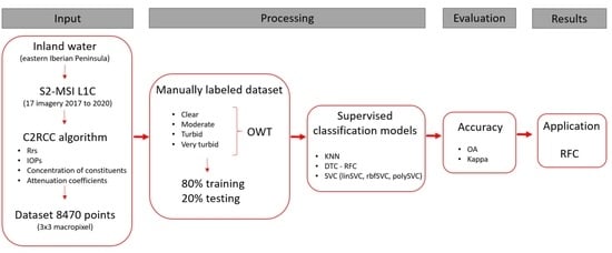
2.2. Processing Sentinel-2 MSI Imagery

The Sentinel-2 mission is part of the Copernicus program, funded by the European Commission and ESA, where the European Space Agency contributes through launching and maintaining the satellites, in addition to collecting and pre-processing the data. The main characteristics of the mission and the MSI instrument can be found on the dedicated ESA Sentinel online web page [23]. In this work, S2-MSI Level-1C (L1C) images are downloaded and processed to Level 2 (L2). The radiometric values per pixel of the L1C are TOA reflectance (top of atmosphere). It is necessary to convert these values to surface reflectance and remove the effect of the atmosphere on the dataset. Although ESA provides products atmospherically corrected with the Sen2Cor processor (Level-2A), the application of a non-specific atmospheric correction (AC) for inland water translates into a less accurate bottom reflectance. For this reason, we use a water-specific AC approach, the Case 2 Regional Coast Colour (C2RCC) algorithm v1.1 [24]. This neural net-based algorithm can be found in SNAP and is easily applied to the L1C images. The C2RCC processor is based on an extensive database of simulated water reflectances and their corresponding TOA radiance, with more than 5 million data. Neural networks are trained to invert the spectrum for the atmospheric correction, deriving from this process the signal from the water (water-leaving radiance) and simultaneously deriving the in-water concentrations from the inherent optical properties (IOPs). C2RCC allows for the conversion of the water-leaving radiances into R${}_{rs}$. A review of the bibliography shows that C2RCC is the atmospheric correction that gives the best results when obtaining information on continental water masses with characteristics similar to those in our study area [2,25,26]. Specifically, in the work of Pereira-Sandoval et al. [22], it was determined that C2RCC obtained the highest coefficients of determination and the lowest deviations in relation to in situ measured reflectance on several of the lakes investigated here (average of $R^2$ of 0.82, RMSE of 0.016, and MAE of 0.011). In another work carried out by Urrego et al. [27], a validation process to assess the performance of biophysical parameters, such as Chl-a and total suspended matter (TSM) concentrations derived from C2RCC applied to S2-MSI imagery, confirmed the good performance of the neural net approach for waters with Chl-a below 10 mg m${}^{-3}$ and TSM lower than 10 mg L${}^{-1}$. The C2RCC allows for the retrieval of 8 of the 12 bands of S2-MSI (R${}_{rs}$), plus the inherent optical properties (IOPs), concentrations of constituent (Chl-a and TSM), and attenuation coefficients ($K_{ds}$).

2.3. Definition of Optical Water Types

An adaptation of the classes proposed by Uudeberg et al. [25,28] and Soomets et al. [2] is used as a basis. The first step involves analyzing the spectral response shape from the set of S2-MSI images corrected by C2RCC. After analyzing the spectral response and using expert knowledge of the biophysical parameters in the lakes of interest, four categories of water types are adapted: clear, moderate, turbid, and very turbid. The category “brown” is discarded because the work of Uudeberg et al. [25] is based on the boreal lakes of Estonia and Latvia, and we did not observe similar ($R_{rs}\left(\lambda \right)$) responses in this particular Mediterranean area for the cases analyzed. The identified and defined types are (Figure 2):

• Clear: The ($R_{rs}\left(\lambda \right)$) signal is weak, with a small peak between 490 and 560 nm. These are waters with low optically active constituent concentrations and high transparency. The higher absorption is in the red and infrared (600–700 nm), and the water appears with very dark or black colors. The content of substances, such as phytoplankton, is possible but in very low quantities. For this class, the Chl-a C2RCC range found is between 0.01 and 14.0 mg m${}^{-3}$, with an average of 2.15 mg m${}^{-3}$, and the TSM values are below 22.2 mg L${}^{-1}$, with an average of 4.3 mg L${}^{-1}$.
• Moderate: The maximum reflectance is located between 560 and 700 nm. Unlike the “Clear” category, the peak is wider due to a higher presence of substances with optical properties, although there is no one particular matter that dominates. If the signal peak is present at wavelengths 600 nm or longer, it can be linked to the presence of Chl-a, though suspended sediments and other Non-Algal Particles (NAP) in small quantities might also be present. For this class, the Chl-a range calculated with C2RCC is between 1.5 and 38 mg m${}^{-3}$, with an average of 19 mg m${}^{-3}$; and the TSM values are between 1.3 and 123 mg L${}^{-1}$, with an average of 65 mg L${}^{-1}$. In our study area, this class has the greatest number of measurements.
• Turbid: The ($R_{rs}\left(\lambda \right)$) peak can be found closer to green and red wavelengths (500–665 nm), with a secondary peak around 700 nm. In general, reflectances are higher in magnitude than they are in the other classes. The main in-water components of this type of water are related to phytoplankton, such as chlorophyll-a pigments. For this class, the C2RCC Chl-a range is between 1.0 and 280 mg m${}^{-3}$, with an average of 17.11 mg m${}^{-3}$; the TSM values can reach 150 mg L${}^{-1}$, with an average of 43 mg L${}^{-1}$. In this case, only 8 measurements have Chl-a values > 200 mg m${}^{-3}$, and they are in correspondence with low TSM values.
• Very Turbid: The highest ($R_{rs}\left(\lambda \right)$) values can be found in longer wavelengths, reaching 740 nm and with a clear signal beyond 800 nm. This large spectral amplitude is due to the high concentrations of suspended sediments, mainly (but not only) to non-organic mineral particles. Waters with large amounts of phytoplankton, such as those caused by massive blooms of cyanobacteria, also cause great turbidity in the water, so this type of case could include two types of water with concentrations from different sources. For this class, the C2RCC Chl-a range can reach 364 mg m${}^{-3}$, with an average of 27 mg m${}^{-3}$, and the TSM values 150 mg L${}^{-1}$, with an average of 114 mg L${}^{-1}$. Only 7 points have Chl-a values > 200 mg m${}^{-3}$, and they are in correspondence with same high TSM values.

2.4. The Sampling Procedure

All the bands obtained from the application of the C2RCC algorithm to the S2-MSI imagery are used as inputs. Thus, a total of 21 bands are used to generate the features: R${}_{rs}$ from B1 to B8 (8); inherent optical properties (IOPs) related to the scattering of light, the backscattering of white ($iop\_bwit$) and other particles ($iop\_bpart$), and the total backscattering ($iop\_btot$) (3); the absorption of the detritus ($iop\_adet$) (1); the total absorption ($iop\_atot$) (1); the absorption of the chlorophyll pigments ($iop\_adg$,$iop\_apig$) (2); the absorption of the yellow substance ($iop\_agelb$) (1); the attenuation coefficients and the depth of the water column from which 90% of the water-leaving irradiance comes ($Kd489$, $kdmin$, and $kd\_z90max$) (3); and the chlorophyll-a and total suspended matter concentrations ($con\_chl$ and $conc\_tsm$) (2).

Seventeen corrected C2RCC S2-MSI images from 2017 to 2020, in different seasons of the year, are used to extract the pixel values centered on 8470 points based on 3 × 3 macropixel extraction, from which screening of valid pixels is performed following [29]. Many of them are randomly selected, others are matched-up to in situ measured reflectance and concentrations (Chl-a, TSM, Secchi disk ($Z_{sd}$), phycocyanin). The spectral signal of the extracted pixels is analyzed together with visual interpretation and the previously acquired knowledge of the dynamics of the lakes, and the pixels are labeled manually.

Figure 2 shows the median values per class calculated on the labeled data. The collection of the samples is carried out using the SNAP software. Python Jupyter Notebooks are developed for the screening of the original macropixels [29] and the calculation of the median, both on the macropixels and the resulting clusters after labeling with the four classes. The database compiled is not balanced: the “moderate” class is the most sampled (nearly 4000 points), in contrast with the “very turbid” with roughly 300 points. The “moderate” and “turbid” classes are more common in our lakes compared with the “clear” and “very turbid” classes. A large part of the data comes from the Albufera lagoon. This water mass is rather round and large, which thus reduces the error introduced by the adjacency effect occurring, especially in pixels closer to the shores, and makes it quite easy to obtain good quality data. However, this lagoon is hypereutrophic and, for most of the year, there is some type of matter in suspension. That is the reason most of the labeled samples were considered “moderate” or “turbid”. On other clearer and narrower water bodies, the effect of adjacency is plausible, which makes it more difficult to obtain reliable samples without a good screening of non-valid pixels. Clear waters have very weak reflectance values, especially at wavelengths greater than 665 nm, and very turbid waters occur only during very specific events, which means they do not have a great recurrence nor is it so easy to obtain good quality data from these lakes.

2.5. Classification Algorithms

In continental waters, the application of classification algorithms for OWT has generally been performed using unsupervised methods [18,30,31,32,33]. The supervised classification approaches used here are based on a training dataset with areas (pixels) known to belong to a certain type of class and which are later used to execute the classification and predict the belonging to a certain class on new data. The a priori knowledge of the dynamics of the lakes and reservoirs of our study area, acquired during field work, observation, and analysis of several types of data, provided a valuable source of information. The classification algorithms used here are framed as the so-called “supervised learning classifiers”. The three most well-known families of algorithms selected are the K-nearest neighbor, decision trees, and support vector machines. According to similar experiences and optimal results obtained by different authors [34,35,36,37], and after evaluating their ease of implementation and their accuracy (see

Table 1. Statistics of the tested models. KNN refers to K-nearest neighbor; DTC, decision tree classifiers; RFC, random forest classifiers; linSVC is the linear support vector classifier; rfbSVC is the non-linear radial basis function (RBF) kernel for the SVC; and polySVC, the polynomial kernel for the SVC.

Classifier Tests
	Specifications	All Bands		Only Rrs
		OA	Kappa	OA	Kappa
KNN	2 neighbors	0.98	0.96	0.96	0.94
DTC		0.96	0.93	0.95	0.91
RFC	max_depth:70; max_leaf:34; min_split:2; n_estimators:430; min_samples_leaf:4	0.96	0.92	0.94	0.90
linSVC	lin (gamma:0.01; C:1000)	0.94	0.89	0.92	0.85
rbfSVC	rbf (gamma:0.1; C:10000)	0.98	0.96	0.96	0.93
polySVC	poly (degree:9)	0.93	0.86	0.91	0.81

), six machine learning approaches are tested: K-nearest neighbor (KNN), decision trees (DTC), random forest (RFC), linear support vector machine (linSVC), radial basis function SVC (rbfSVC), and polynomial SVC (polySVC).

• The K-nearest neighbor (KNN) is very easy to implement and does not require training prior to making the predictions, thus reducing computing times. It calculates the distance of a new data point to all other data points using selected approaches (Euclidean, Manhattan, etc.). K is the number of points with the least distance to the new point. These new data are assigned to the class to which the majority of the K-nearest points belong. The main disadvantage of this classifier is that it can fail if there are too many dimensions (large dataset). K is selected after testing and evaluation, with K = 5 being quite common in the literature, though some testing can be performed to determine which value is recommended for a specific dataset.
• Among decision trees, we selected the basic expression (DTC here) and the random forest classifier (RFC) [38]: RFCs are classical algorithms based on the ensemble of hundreds or thousands of classification trees. The main idea of RFC is that the results obtained by averaging simple classifiers (trees in this case) can obtain better results than the ones obtained by single, more sophisticated, and powerful classifiers. Important and relevant features of DTC and RFC are that they are fast to train and in making predictions; that they are easily parallelizable, making them especially suitable for new hardware composed of multi-core systems; and that they provide a feature ranking (or variable importance) which indicates the most influential features. They are known for obtaining quite good results for remote sensing classification problems.
• The support vector machine for classification, SVC [39], is a well-established, state-of-the-art algorithm for nonlinear binary and multiclass classification. It works by mapping the input (training) samples into a high-dimensional Hilbert space using a (in principle unknown) nonlinear function where a linear classification is performed by defining a hyperplane that separates the different classes with maximum margin. The most relevant characteristics of this type of classifiers are that (i) they obtain a sparse solution where only the most relevant training samples are used, which are called support vectors; (ii) they are able to deal with noisy input samples; (iii) they generalize well, i.e., they are able to make good predictions on new, unseen samples; and (iv) they are relatively fast to train, and once a model is obtained, very fast for making predictions on new input samples.

The accuracy of the algorithms is measured by means of the overall accuracy (OA) and the Cohen’s Kappa values (Kappa). The overall accuracy is expressed as the sum of the number of correctly classified values divided by the total number of values. The correctly classified values are located along the upper-left to lower-right diagonal of the confusion matrix. The total number of values is the number of values in either the truth or predicted-value arrays. If the entire set of predicted labels for a sample strictly match with the true set of labels, then the subset accuracy is 1.0; otherwise, it is 0.0 (scikit-learn.org (accessed on 1 January 2020)):

$$accuracy(y,\widehat{y})=\frac{1}{n_{samples}}{\displaystyle \sum _{i=0}^{n_{samples}-1}}1({\widehat{y}}_i=y_i)$$

(1)

where ($y,\widehat{y}$) are the measured and the predicted values, respectively.

The Kappa statistic (or value) is a metric that compares observed accuracy with expected accuracy (random chance). The Kappa statistic is used not only to evaluate a single classifier but also to evaluate classifiers amongst themselves. In addition, it takes into account random chance (agreement with a random classifier), which generally means it is less misleading than simply using accuracy as a metric. Computation of observed and expected accuracy is integral to comprehending the Kappa statistic and is most easily illustrated through the use of a confusion matrix.

$$Kappa=(observed\_accuracy-expected\_accuracy)/(1-expected\_accuracy)$$

(2)

Landis and Koch [40] considered a Kappa of range 0–0.20 as slight, 0.21–0.40 as fair, 0.41–0.60 as moderate, 0.61–0.80 as substantial, and 0.81–1 as almost perfect agreement. The role of the Kappa value in this work is to serve as an auxiliary indicator for accuracy. Limitations of this value have been reported by [41].

3. Results

As has been mentioned, one of the main objectives of this work is to test different classifiers and see how they distribute each category during different events and on various lakes and reservoirs of the study area. The classifications generated can help better understand the seasonal and spatial variations of the water masses being studied and can serve as a basic support in the monitoring programs of lakes and reservoirs. In addition to being used as a final product, classifications can also be considered an intermediate product that helps in the subsequent selection of the water quality data extraction algorithm generated and adapted to specific types of water [20].

3.1. Comparison of Classifiers

Several tests are performed using the Python scikit-learn classifiers package. The original dataset is split into the training and test sets: 80%, or 6776 data points and 21 bands, are used for training; and 20%, or 1694 data points, are used for testing. To evaluate the performance of the classifiers, the overall accuracy (OA), Kappa, and confusion matrices are calculated. The input features are standardized when specific classifiers needed the data in similar ranges (KNN and SVC classifiers). The variety of the bands in the set is quite large because we used not only the information provided by the reflectances but also the IOPs and concentrations calculated by the C2RCC algorithm. Table 1 shows the accuracy of the various classifiers implemented. We also test whether exclusively using the $R_{rs}$ would also lead to good results.

The statistics show that using all 21 features gives better metrics in general, even if the differences when using only the R${}_{rs}$ are not striking. The training and processing times do not change dramatically, which is the reason we consider training the models with all the available information, assuming some redundancy. The configuration by the model is performed by tackling some of the hyperparameters (see “specifications” in Table 1). See Annex A to gain deeper knowledge on how this was conducted. The confusion matrices for all the models are also derived.

Table 2. Confusion matrix of RFC with all bands. EC is error of commission; EO is error of omission; PA is the producer’s accuracy; UA is the user’s accuracy.

	Predicted
Real	Clear	Moderate	Turbid	Very Turbid	Total	EC	PA
clear	206	2	3	0	211	0.02	0.98
moderate	21	1044	17	0	1082	0.04	0.96
turbid	10	3	333	14	360	0.07	0.93
very turbid	3	0	3	35	41	0.15	0.85
Total	240	1049	353	49
EO	0.14	0.0	0.06	0.29
UA	0.86	1.0	0.94	0.71
Overall accuracy						1694	0.96

shows the confusion matrix of the RFC model. The confusion matrix was generated with the test dataset. As mentioned before, the input dataset is separated into a training set (80%), for the learning process of the models, and the test set (20%), an independent group of data used exclusively to check the algorithm performance. The test data are then classified by the model, and the comparison with the labeled data is performed by class in a confusion matrix. The results of the predictions (“Predicted”) are compared with the control (“Real”) or test. The overall accuracy is quite high (0.96), but we see that the commission and omission errors of the class “very turbid” are higher than those of the other classes (0.29 and 0.15). This is also visible for the other classifiers, for instance, the DTC confusion matrix shows a producer’s accuracy (PA) of 0.86 (not shown here) for the “very turbid” class (see

Table A1. Confusion matrix KNN with all bands. EC is error of commission; EO is error of omission; PrAc is the producer’s accuracy; UsAc is the user’s accuracy.

Predicted
Real	Clear	Moderate	Turbid	Very Turbid	Total	EC	PrAc
clear	196	8	7	0	211	0.07	0.93
moderate	11	1069	2	0	1082	0.01	0.99
turbid	4	2	350	4	360	0.03	0.97
very turbid	5	3	7	26	41	0.37	0.63
Total	223	1080	354	36
EO	0.08	0.01	0.04	0.13
UsAc	0.91	0.99	0.96	0.87
Total accuracy						1694	0.97

in Appendix A for the KNN).

3.2. Feature Importance

The RFC and the SVC linear and radial basis function (RBF) kernel allow us to check for the relevance of each feature used as input in the classifications [42]. This analysis is performed by calculating the increase in the model’s prediction error after permuting that specific feature. The permutation importance of a feature uses a baseline metric, defined by scoring, that is evaluated on a dataset defined by the X. Next, a feature column from the validation set is permuted and the metric is evaluated again. The permutation importance is defined to be the difference between the baseline metric and the metric from permutating the feature column. If this change in value makes the error increase, the feature is relevant because the model relied on it more for the prediction. Figure 3 shows the importance of each of the 21 features for the RFC model: the reflectances in the range from blue to green (B1–B3, 443–560 nm), together with the near infrared (B8A, 864 nm) appear as relevant as the scattering IOPs ($iop\_bwit$ and $iop\_bpart$) and the absorption IOPs ($iop\_adet$ and $iop\_atot$). The matter concentrations ($conc\_chl$ and $conc\_tsm$) and the bands in the red part of the spectrum (B4–B7, 664–780 nm) are less significant.

The SVC (linear and RBF) feature importance is also derived, and the plots are available in Appendix B (Figure A3). There are some differences between the kernels used. The linear SVC (linSVC) gives more weight to the first four reflectance bands, followed by the scattering IOPs, while in the RBF (rfbSVC), the absorption IOPs have a more prominent role, with the IOPs related to the scattering of light ($iop\_bwit, iop\_bpart$, and $iop\_btot$), together with the absorption of the detritus ($iop\_adet$), the total absorption ($iop\_atot$), and the absorption of the chlorophyll pigments ($iop\_adg$ and $iop\_apig$) being the most relevant features. The reflectances seem to have a strong weight too, highlighting bands B2 (490 nm) and B3 (560 nm), followed by B1 (443 nm). The in-water concentrations of the total suspended matter and chlorophyll-a ($conc\_tsm$ and $conc\_chl$) seem to be less significant. The depth of the penetration of light ($Kd\_z90max$) and the absorption of the yellow substance ($iop\_agelb$) seem to be less suited to this four-class classification. This can be partially explained by the lack of training data related to the CDOM absorption-dominant lakes, which are not represented in our training dataset.

3.3. Application of Classifiers: Performance in Contreras Reservoir

We apply the classification approaches to the lakes in the study area. As an example, we show in Figure 4 the results of the classifications using the KNN, DTC, and RFC and the three tested SVC kernel (linear, RBF, and polynomial) classifiers on the Contreras reservoir on 11 May 2019. In Figure 5, the Chl-a and TSM derived from the C2RCC algorithm are also shown on the same day for reference. The first thing we should remark is that an area in the southeastern part of the lake considered to be water is in reality the shadow of a cloud, and it shows an error on the screening of non-valid pixels when the C2RCC is applied. The four algorithms show three classes in the lake, but there are obvious differences. The DTC and RFC results are similar, with the DTC being a bit more noisy. The DTC classifies the pixels of the SE as Class 3, while the RFC assigns those pixels to Class 1 or Class 2. The SVC results differ from them, with a dominance of Class 1 or “Clear” in the linear kernel, except in the northern part, while the rfbSVC and the polynomial kernel detect the turbidity in the SE part in a way more similar to the DTC and RFC. It is surprising to see that the shadowy area in the SE has been classified as “Turbid” or Class 3 by the rfbSVC. The KNN gives similar results to the polySVC in the central and SE areas of the lake but classifies the northern part as in the DTC and RFC (the “Turbid” and “Moderate” classes are found). With a visual analysis alone, it is difficult to establish which classification gives results closer to reality, and we cannot really determine which one is better for all areas of the lake and for all the images analyzed.

Fortunately, the Contreras reservoir has been monitored by the University of Valencia on several field campaigns since 2017 (February 2017, May 2017, November 2017, June 2018, and September 20018). Among the biophysical parameters measured in situ, Chl-a, the content of the sediments, and the Secchi disk depth ($Z_{sd}$) measurements have been carried out. During these campaigns, the reservoir has presented low values of Chl-a (less than 2.5 mg m${}^{-3}$), a Secchi disk between 0.95 and 4.5 m; and a range of sediment concentrations between 1.45 and 28 mg L${}^{-1}$. According to these, the Contreras waters have been classified as ultraoligotrophic to oligotrophic throughout the year, with occasional cases of mesotrophic to eutrophic. In order to verify the separation in the area/classes made by the classifiers, we have matched those different areas with the Chl-a and TSM products derived from the C2RCC algorithm for our complete time series (Figure 6). The lake is separated into four areas: North, Center, South–Center, and South–East. In each area, a series of points are marked and the average values of the Chl-a and TSM are extracted for the available days. Focusing on the day analyzed in this example, in the N area, the values of Chl-a are 6.8 mg m${}^{-3}$ on average, and the TSM is 14.38 mg L${}^{-1}$ on average. In the central area (C), Chl-a reaches values of 2.4 mg m${}^{-3}$ and TSM 4.1 mg L${}^{-1}$. In the SC area, the Chl-a has a 3.5 mg m${}^{-3}$ average and TSM 7.3 mg L${}^{-1}$. Finally, the SE area shows Chl-a average values of 6.1 mg m${}^{-3}$ and TSM of 14.5 mg L${}^{-1}$. From these results, we can infer that the classes derived by the RFC classifier are closer to the real case than the classifications made by the other approaches. We have obtained good statistics results with the RFC, and we are able to obtain information about the relevance of the bands in the model, thus making the approach a bit more explainable. Other studies have also found the RFC to be the best classifier for various types of datasets, followed closely by SVCs [43,44]. In addition, the RFC is scale invariant and does not require pre-processing, whereas the SVC needs scaling and normalization of the datasets. The RFC is computationally complex, but less so than the SVCs, in addition to being highly tunable. Bearing all these reasons in mind, we used the RFC for the time-series analysis of the status of three other lakes apart from the Contreras: the Sotonera and Mediano reservoirs and the Albufera lagoon.

3.4. Time-Series Analysis

The use of a time series of OWTs can help visualize possible changes to later apply the proper in-water algorithms in the retrieval of the concentration of the different components (e.g., Chl-a, TSM, and CDOM) based on specific water types. Four water bodies are analyzed here using the RFC results: the Sotonera, Contreras, and Mediano reservoirs and the Albufera lagoon. We have selected several days over 2019 as a representation of the four seasons of the Mediterranean climate. Figure 7 shows the results obtained by applying the RFC in the Sotonera reservoir. This water body is nourished by the waters of the Gállego Canal and the Sotón River, of very different origins, so the composition of its waters is also highly variable. The reservoir is intensively used for irrigation and human consumption, making its level very unstable, dropping down to 10 m in the summer [45], which, in addition to some strong slopes in its margins, generates a high risk of erosion in the catchment area of the lake. The result of the erosion and transport of materials ends up producing large TSM volumes in the water. The effect of these sediments on the water quality can be easily seen: there is not one image in which we cannot see turbidity in the water. Although officially it is considered mesotrophic [45], which indicates the possible development of biological communities, the high turbidity of the water by suspended inorganic particulates prevents greater trophic development, as it should be according to its levels of nutrients. The image on 3 February shows a turbid mass (Class 3) throughout the reservoir; on 26 May, there is a predominance of Class 1 at the south (clear water) while the area on the north appears turbid (Class 3). On 15 July, the turbidity class has extended to the south, and according to the auxiliary information, there is a high content of Chl-a. Finally, on 26 October, we see the lowest water level of the lake after a rather dry summer. Turbid Class 3 covers the water mass.

The time-series plot on the Contreras reservoir (Figure 8) tells a different story. It is one of the most optically stable water masses studied here, with predominantly clear or moderate waters due to its oligotrophic state, in which the regularly low Chl-a content (lower than 2.5 mg m${}^{-3}$) does not affect it enough to change the water into the turbid types in most cases. Occasionally, there is an input of large amounts of sediment during events of precipitation and runoff. For instance, from 19 to 21 December 2019, a rainfall episode of great magnitude dragged a huge quantity of materials from the surrounding slopes, which ended up in the Cabriel riverbed and brought a significant amount of particulates into the waters of the Contreras reservoir. This type of event leads to an important modification in the dynamics and ecological state of the water. In the current context of climate change, in which the increase in the frequency, intensity, and seasonal variability of extreme rainfall events is proven [46,47], a high recurrence of events of this type can lead to the modification of ecological thresholds. These thresholds are conditioned not only by the availability of nutrients but also by the usual optical properties and the development of biological communities in the photic zone. With increased sediment and reflectance of the waters, the photic zone, of vital importance for primary production, decreases in depth, modifying the bio-optical conditions and therefore possibly destroying the adapted biological communities and inducing a change in the trophic state of the waters. This type of analysis was also performed on the Mediano reservoir (Figure 8, right), where the behavior is similar to Contreras, because both are at the head of river courses. Here, the contributions of the sediments and materials surrounding the lakes are important, but seasonal. However, sediment enters the Mediano more frequently and with more evident color changes. During the summer (4 August 2019) and autumn (12 November 2019), Class 3 seems to be dominant. The values of Chl-a are not high enough, which indicates that the main concentration of the TSM reaching this reservoir consists of particles of minerals of inorganic origin (SPIM, Suspended Particulate Inorganic Matter). The fact that the reservoir is located at the head of the river prevents the arrival of nutrients of anthropogenic origin, so in this type of reservoir, the turbidity is closely related to sediment clogging rather than to problems of bacteria or eutrophication. A common pattern that we can establish between the Contreras and Mediano reservoirs is that, in both, the turbid-type water values increase throughout the summer, with its maximum presence in the month of August due to the typical summer storms in this area of the Mediterranean.

The Albufera lagoon is a special case, where cyanobacteria is the dominant taxonomic class of phytoplankton. The Albufera is located south of the city of Valencia, between the mouths of the Turia and Jucar rivers, with an area of 2500 ha and an average depth of 1–3 m [48]. It is one of the most important wetlands in the western Mediterranean. Three ecosystems can be differentiated: the lake, which gives the park its name; the marsh and its rice fields (14,500 ha); and the Devesa sandbank that separates the lake and the sea. However, its location, surrounded by the metropolitan area of Valencia and a large area of rice fields, traced by a network of ditches and canals, results in an excessive input of nutrients, fertilizers, and urban and industrial discharges that, together with the decrease in the flow of water entering the lagoon from its hydrographic basin due to climatic change conditions coupled with the increase in water concessions in the upper areas of the Jucar River, poses a growing threat to this emblematic space. A hypertrophic state is manifested in an explosion of phytoplankton that greens and darkens the water, in recurrent cycles of anoxia and in a radical fall in fish production, particularly of the species of greatest commercial value. Its dynamics follow patterns that depend on surface inputs and the management of the water system according to the needs of the rice crops that surround it. The average annual Chl-a since the late 1980s is 150–160 mg m${}^{-3}$. In the images shown in Figure 9, we can observe the water covering the rice fields surrounding the lake at the beginning of the year. The rice fields are flooded in November and stay covered by water until the end of February when the gorges, until now closed, are opened and the fields dry. The water classes on 11 January 2019 are classified from moderate to very turbid. As mentioned earlier, the water level is about 20 cm above the annual average and the fields below the lagoon level are flooded to promote the decomposition of organic remains. In the summer, the turbid class (Class 3) seems to be dominant. Sòria-Perpinyà et al. [48] carried out a study about the presence of phycocyanin during 2016 and 2017 and determined that phycocyanin presents a strong decline in the summer period, which indicates a decrease in the primary production motivated by the depletion of nutrients after the production peak in the late spring.

4. Discussion

Examining the results obtained using the different classifiers, we see that the OWT supervised classifications show good statistics in general, with pixels assigned into the four defined classes with more or less accuracy. However, we are aware that knowing the actual constituents of the water at any one determined moment is not so straightforward because similar spectral curves may indicate different compositions or constituents in the water. This makes it complex to quickly infer the process or processes that can affect the water masses.

One of the main weaknesses of the database generated here is that it is only based on very good, easily classifiable spectral curves. However, nature usually does not respond to such defined patterns. The collection of the training samples and the manual labeling process were performed mainly in one year (2019) on different lakes but with a clear dominance of the samples taken for the “moderate” class (Class 2). This was partially corrected when the models were trained because the SVCs and RFC allow the classes to be balanced internally.

It is also sometimes difficult to distinguish between moderate and turbid waters because the only thing distinguishing these two classes is a higher magnitude of the signal peak at 560 nm. The various tests performed on the types and number of inputs of the training models were conducted solely to examine how a classifier with a higher quantity of input data but with less specific characterization of each sample would behave in comparison with a classifier with less data but a better water characterization (i.e., adding IOPs, concentrations, and geometries). What became clear is that thanks to the biophysical parameters derived by the C2RCC algorithm, the more highly detailed water characterization greatly facilitated the distinction of the water types, especially when very similar spectral curves were obtained, corresponding to different constituents in the water. For instance, although two bodies of water can be classified as very turbid, knowing the chlorophyll content derived by the C2RCC made it possible to determine if the turbid event is produced by decaying algal blooms or if it is only being produced by suspended inorganic particulate matter. We can venture that the addition of auxiliary information, such as the contents in suspended particulate organic matter (SPOM) or phycocyanin, could be helpful for making further distinctions of more water types.

We cannot really draw a conclusion as to the most appropriate supervised classifier based on the statistics or the analysis made on the images. In some cases, one model works better than the others, but the results change within different water masses. We decided to use the RFC for several reasons: the strong literature support, how easily understood it is compared to other complex models, and finally, because it is possible to tune the hyperparameters to make it more adjustable to the input database, thus avoiding overfitting. The RFC can handle binary features, categorical features, and numerical features. Very little pre-processing needs to be performed because there is no need to scale or transform the features. The feature importance permutation analysis is also a relevant reason for selecting this model as it makes the results a bit more understandable. Other reasons are: it works very well with high dimensionality; it is parallelizable (faster computation time); training times are fast; it handles unbalanced data, thus minimizing the overall error rate; and each decision tree in the forest has a high variance but low bias. Concerning this last point, all the trees in the random forest are averaged and, consequentially, the variance is averaged as well, so we obtain a low bias and a moderate variance model.

The OWT classification can be used as a final product for the analysis of water changes [18], or as an intermediate step for selecting the in-water algorithm, or even the most appropriate atmospheric correction for each water type [49]. Ideally, the OWT classification should be performed on non-atmospherically corrected data, which would save time and loops in the processing of large datasets. Work is being done in this direction, testing the bottom of the Rayleigh reflectance as input instead of the fully corrected L2 data.

5. Conclusions

A classification of optical water types, as a monitoring or diagnostic tool of the initial state of water bodies, has been implemented here. We have trained several supervised classification models (the KNN, DTc, and RFC and variations of SVCs) with a manually labeled dataset with four different water types. The features for the identification of the four classes were based on the spectral curves and the information derived from IOPs and concentrations calculated by the C2RCC neural net over Sentinel-2 images. The ability to apply supervised classification algorithms to obtain the OWT has been demonstrated, achieving optimal results in lakes and reservoirs with different levels of complexity in the SE of the Iberian Peninsula. Although the statistical results of the different classifiers are very similar, the RFC model has been the one selected for the processing of the time series. The analysis of the OWT time series of several lakes has been used to validate the classification results, in comparison with the expected dynamics of the water masses. The information provided by the OWT can be used as a final product, for instance, for detecting different types of algae blooms or water dynamics. It can also be used as an intermediate product for gaining further knowledge on the status of the water and for generating more accurate reflectance or water quality concentration parameters. Future work will be focused on enhancing the labeled dataset. To achieve this, more work must be done for the manual labeling, continuing with the methodology used here. Trying online machine learning models is another possibility, in which data become available in a sequential order and are used to update the best predictor/classifier for future data at each step (incremental learning [50]). Another topic of interest is the knowledge transfer on lakes with similar characteristics in other geographical regions, e.g., Lake Balaton in Hungary, or testing the models on more extreme water masses, such as the Mar Menor in Murcia (Spain), for different times of the year and conditions.

References

1. European Parliament 2000. Available online: https://ec.europa.eu/environment/water/water-framework/index_en.html (accessed on 8 May 2022).
2. Soomets, T.; Uudeberg, K.; Jakovels, D.; Zagars, M.; Reinart, A.; Brauns, A.; Kutser, T. Comparison of Lake Optical Water Types Derived from Sentinel-2 and Sentinel-3. Remote Sens. 2019, 11, 2883. [Google Scholar] [CrossRef] [Green Version]
3. Copernicus Global Land Service. Available online: https://land.copernicus.eu/global/products/lwq (accessed on 8 May 2022).
4. Odermatt, D.; Danne, O.; Philippson, P.; Brockmann, C. Diversity II water quality parameters for 300 lakes worldwide from ENVISAT (2002–2012): A new global information source for lakes. Earth Syst. Sci. Data 2018, 10, 1527–1549. Available online: https://essd.copernicus.org/articles/10/1527/2018/ (accessed on 8 May 2022). [CrossRef] [Green Version]
5. Reinart, A.; Paavel, B.; Tuvikene, L. Effect of coloured dissolved organic matter on the attenuation of photosynthetically active radiation in Lake Peipsi. Proc. Est. Acad. Sci. Biol./Ecol. 2004, 53, 88–105. [Google Scholar]
6. Mañosa, S.; Mateo, R.; Guitart, R. A review of the effects of agricultural and industrial contamination on the Ebro Delta biota and wildfire. Environ. Monit. Assess. 2001, 71, 187–205. [Google Scholar] [CrossRef]
7. Soria, J.M. Past, present and future of la Albufera of Valencia Natural Park. Limnetica 2006, 25, 135–142. [Google Scholar] [CrossRef]
8. Serrano, L.; Reina, M.; Martín, I.; Reyes, A.; Arechederra, D.L.; Toja, J. The aquatic systems of Doñana (SW Spain): Watersheds and frontiers. Limnetica 2006, 25, 11–32. [Google Scholar] [CrossRef]
9. Soria, J.M.; Caniego, G.; Hernández-Sáez, N.; Dominguez-Gomez, J.A.; Erena, M. Phytoplankton Distribution in Mar Menor Coastal Lagoon (SE Spain) during 2017. J. Mar. Sci. Eng. 2020, 8, 600. [Google Scholar] [CrossRef]
10. Sòria-Perpinyà, X.; Vicente, E.; Urrego, P.E.; Pereira-Sandoval, M.; Tenjo, C.; Ruiz-Verdú, A.; Delegido, J.; Soria, J.M.; Peña, R.; Moreno, J. Validation of Water Quality Monitoring Algorithms for Sentinel-2 and Sentinel-3 in Mediterranean Inland Waters with In Situ Reflectance Data. Water 2021, 13, 686. [Google Scholar] [CrossRef]
11. Romo, S.; García-Murcia, A.; Villena, M.J.; Sánchez, V.; Ballester, A. Tendencias del fitoplancton en el lago de la Albufera de Valencia e implicaciones para su ecología, gestión y recuperación. Limnetica 2008, 27, 11–28. [Google Scholar] [CrossRef]
12. Romo, S.; Soria, J.; Fernández, F.; Ouahid, Y.; Barón-Solá, A. Water residence time and the dynamics of toxic cyanobacteria. Freshw. Biol. 2013, 58, 513–522. [Google Scholar] [CrossRef]
13. Global Lakes Sentinel Services. Available online: https://un-spider.org/es/links-and-resources/gis-rs-software/glass-global-lakes-sentinel-services (accessed on 8 May 2022).
14. Diversity II. Available online: http://www.diversity2.info/ (accessed on 8 May 2022).
15. CyanoAlert. Available online: https://www.cyanoalert.com/ (accessed on 8 May 2022).
16. Sentinel Application Platform. Available online: https://step.esa.int/main/download/snap-download/ (accessed on 8 May 2022).
17. Moore, T.S.; Campbell, J.W.; Feng, H. A fuzzy logic classification scheme for selecting and blending ocean color algorithms. IEEE Trans. Geosci. Remote Sens. 2001, 39, 1764–1776. [Google Scholar] [CrossRef]
18. Moore, T.S.; Dowell, M.; Bradt, S.; Ruiz-Verdú, A. An optical water type framework for selecting and blending retrievals from bio-optical algorithms in lakes and coastal waters. Remote Sens. Environ. 2014, 143, 97–111. [Google Scholar] [CrossRef] [PubMed] [Green Version]
19. Le, C.; Li, Y.; Zha, Y.; Sun, D.; Huang, C.; Zhang, H. Remote estimation of chlorophyll a in optically complex waters based on optical classification. Remote Sens. Environ. 2011, 115, 725–737. [Google Scholar] [CrossRef]
20. Elveld, M.A.; Ruescas, A.B.; Hommersonm, A.; Moore, T.S.; Peters, S.W.M.; Brockmann, C. An optical classification tool for Global Lake Waters. Remote Sens. 2017, 9, 420. [Google Scholar] [CrossRef] [Green Version]
21. Pereira-Sandoval, M.; Urrego, P.E.; Ruiz-Verdú, A.; Tenjo, C.; Delegido, J.; Sorià-Perpinyà, X.; Vicente, E.; Soria, J.M.; Moreno, J. Calibration and validation of algorithms for the estimation of chlorophyll-a concentration and Secchi depth in inland water with Sentinel-2. Limnetica 2019, 38, 471–487. [Google Scholar] [CrossRef]
22. Pereira-Sandoval, M.; Ruescas, A.; Urrego, P.E.; Ruiz-Verdú, A.; Delegido, J.; Tenjo, C.; Sorià-Perpinyà, X.; Vicente, E.; Soria, J.M.; Moreno, J. Evaluation of atmospheric correction algorithms over Spanish inland waters for Sentinel-2 Multispectral Imagery Data. Remote Sens. 2019, 11, 1469. [Google Scholar] [CrossRef] [Green Version]
23. Sentinel-2. Sentinel Online. Available online: https://sentinel.esa.int/web/sentinel/missions/sentinel-2 (accessed on 8 May 2022).
24. Brockmann, C.; Doerffer, R.; Peters, M.; Stelzer, K.; Embacher, S.; Ruescas, A. Evolution of C2RCC neural network for Sentinel 2 and 3 for the retrieval of ocean colour products in normal and extreme optically complex waters. In Proceedings of the Living Planet Symposium 2016, Prague, Czech Republic, 9–13 May 2016; Available online: http://step.esa.int/docs/extra/Evolution%20of%20the%20C2RCC_LPS16.pdf (accessed on 8 May 2022).
25. Uudeberg, K.; Ansko, I.; Poru, G.; Ansper, A.; Reinart, A. Using optical water types to monitor changes in optically complex inland and coastal waters. Remote Sens. 2019, 11, 2297. [Google Scholar] [CrossRef] [Green Version]
26. Warren, M.A.; Simis, S.G.H.; Martinez-Vicente, V.; Poser, K.; Bresciani, M.; Alikas, K.; Spyrakos, E.; Giardino, C.; Ansper, A. Assessment of atmospheric correction algorithms for the Sentinel-2A MultiSpectral Imager over coastal and inland waters. Remote Sens. Environ. 2019, 225, 267–289. [Google Scholar] [CrossRef]
27. Urrego, E.P.; Delegido, J.; Tenjo, C.; Ruiz-Verdú, A.; Soriano-Gonzalez, J.; Pereira-Sandoval, M.; Sorià-Perpinyà, X.; Vicente, E.; Soria, J.M.; Moreno, J. Validation of chlorophyll-a and total suspended matter products generated by C2RCC processor using Sentinel-2 and Sentinel-3 satellites in inland waters. In Proceedings of the XX Congress of the Iberian Association of Limnology, Murcia, Spain, 26–29 October 2020. [Google Scholar]
28. Uudeberg, K.; Aavaste, A.; Köks, K.L.; Ansper, A.; Uusöe, M.; Kangro, K.; Ansko, I.; Ligi, M.; Toming, K.; Reinart, A. Optical Water Type Guided Approach to Estimate Optical Water Quality Parameters. Remote Sens. 2020, 12, 931. [Google Scholar] [CrossRef] [Green Version]
29. Bailey, S.W.; Werdell, P.J. A multi-sensor approach for the on-orbit validation of ocean color satellite data products. Remote Sens. Environ. 2006, 102, 12–23. [Google Scholar] [CrossRef]
30. Shi, K.; Li, Y.; Li, L.; Lu, H.; Song, K.; Liu, Z.; Xu, Y.; Li, Z. Remote chlorophyll-a estimates for inland waters based on a cluster-based classification. Sci. Total. Environ. 2013, 444, 1–15. [Google Scholar] [CrossRef] [PubMed]
31. Bi, S.; Li, Y.; Xu, J.; Liu, G.; Song, K.; Mu, M.; Liu, H.; Miao, S.; Xu, J. Optical classification of inland waters based on an improved Fuzzy C-Means method. Opt. Express 2019, 27, 34838–34856. [Google Scholar] [CrossRef] [PubMed]
32. Botha, E.J.; Anstee, J.M.; Sagar, S.; Lehmann, E.; Medeiros, T.A.G. Classification of Australian Water bodies across a Wide Range of Optical Water Types. Remote Sens. 2020, 12, 3018. [Google Scholar] [CrossRef]
33. Du, Y.; Song, K.; Liu, G. Monitoring Optical Variability in Complex Inland Waters Using Satellite Remote Sensing Data. Remote Sens. 2022, 14, 1910. [Google Scholar] [CrossRef]
34. Bourel, M.; Crisci, C.; Martinez, A. Consensus methods based on machine learning techniques for marine phytoplankton presence-absence prediction. Ecol. Inform. 2017, 42, 46–54. [Google Scholar] [CrossRef]
35. Chou, J.-S.; Ho, C.-C.; Hoang, H.-S. Determining quality of water in reservoir using machine learning. Ecol. Inform. 2018, 44, 57–75. [Google Scholar] [CrossRef]
36. Watanabe, F.S.Y.; Miyoshi, G.T.; Rodrigues, T.W.P.; Bernardo, N.M.R.; Rotta, L.H.S.; Alcântara, E.; Imai, N.N. Inland water’s trophic status classification based on machine learning and remote sensing data. Remote Sens. Appl. Soc. Environ. 2020, 19, 100326. [Google Scholar] [CrossRef]
37. Grendaite, D.; Stonevicius, E. Machine Learning Algorithms for Biophysical Classification of Lithuanian Lakes Based on Remote Sensing Data. Water 2022, 14, 1732. [Google Scholar] [CrossRef]
38. Ho, T.K. Random decision forests. In Proceedings of the 3rd International Conference on Document Analysis and Recognition, Montreal, QC, Canada, 14–16 August 1995; Volume 1, pp. 278–282. [Google Scholar] [CrossRef]
39. Cortes, C.; Vapnik, V. Support-vector networks. Mach. Learn. 1995, 20, 273–297. [Google Scholar] [CrossRef]
40. Landis, J.R.; Koch, G.G. The measurement of observer agreement for categorical data. Biometrics 1977, 33, 159–174. [Google Scholar] [CrossRef]
41. Pontius, R.G., Jr.; Millones, M. Death to Kappa: Birth of quantity disagreement and allocation disagreement for accuracy assessment. Int. J. Remote Sens. 2011, 32, 4407–4429. [Google Scholar] [CrossRef]
42. Breiman, L. Random forests. Mach. Learn. 2001, 45, 5–32. [Google Scholar] [CrossRef] [Green Version]
43. Fernandez-Delgado, M.; Cernadas, E.; Barro, S. Do we need hundreds of classifiers to solve real world classification problems? J. Mach. Learn. Res. 2014, 15, 3133–3181. [Google Scholar]
44. Park, J.W.; Korosov, A.A.; Babiker, M.; Won, J.S.; Hansen, M.W.; Kim, H.C. Classification of sea ice types in Sentinel-1 synthetic aperture radar images. Cryosphere 2020, 14, 2629–2645. [Google Scholar] [CrossRef]
45. Confederación Hidrográfica del Ebro. Diagnóstico y Gestión Ambiental de Embalses en el ámbito de la Cuenca Hidrográfica del Ebro; Ministerio de Medio Ambiente: Embalse de la Sotonera, Spain, 1996; Available online: https://www.chebro.es/documents/20121/48992/Informe_Final_Embalse_de_la_Sotonera_1996.pdf/b4844842-a49b-209b-96a6-7bb799d125af (accessed on 8 May 2022).
46. Dourte, D.R.; Fraisse, C.W.; Bartels, W.L. Exploring changes in rainfall variability in the Southeastern U.S.: Stakeholder engagement, observations, and adaptation. Clim. Risk Manag. 2015, 7, 11–19. [Google Scholar] [CrossRef] [Green Version]
47. Yilmaz, A.; Hossain, I.; Perera, B. Effect of climate change and variability on extreme rainfall intensity-frequence-duration relationship: A case study of Melbourne. Hydrol. Earth Syst. Sci. 2014, 18, 4065–4076. [Google Scholar] [CrossRef] [Green Version]
48. Sorià-Perpinyà, X.; Vicente, E.; Urrego, P.; Pereira-Sandoval, M.; Ruiz-Verdú, A.; Delegido, J.; Soria, J.M.; Moreno, J. Remote sensing of cyanobacterial blooms in a hyoertrophic lagoon (Albufera of València, Eastern Iberian Peninsula) using multitemporal Sentinel-2 images. Sci. Total. Environ. 2020, 698, 134305. [Google Scholar] [CrossRef]
49. Stelzer, K.; Simis, S.; Selmes, N.; Muller, D. Copernicus Global Land Operations “Cryosphere and Water CGLOPS-2”. Product User Manual. Framework Service Contract N° 199496 (JRC). 2020. Available online: https://land.copernicus.eu/global/sites/cgls.vito.be/files/products/CGLOPS2_PUM_LWQ100_S2_v1.2.0_I1.03.pdf (accessed on 8 May 2022).
50. Geng, X.; Smith-Miles, K. Incremental Learning. In Encyclopedia of Biometrics; Springer: Boston, MA, USA, 2009. [Google Scholar] [CrossRef]
Figure 1. Map of the location of the water bodies used to obtain samples. (1) Albufera lagoon. (2) Bellús reservoir. (3) Benagéber reservoir. (4) Beniarrés reservoir. (5) Contreras reservoir. (6) Maria Cristina reservoir. (7) Mediano reservoir. (8) Regajo reservoir. (9) Sitjar reservoir. (10) Toba reservoir. (11) Tous reservoir. Source: IGN and Sentinel-2 cloudless, 2019.
Remotesensing 14 05568 g001
Figure 2. Spectral response of each type of OWT obtained from the average value of all training samples collected.
Remotesensing 14 05568 g002
Figure 3. Feature importance derived from RFC.
Remotesensing 14 05568 g003
Figure 4. Comparison of the models in one image, 11 May 2019, Contreras reservoir: left top, KNN; right top, DTC; left center, RFC; right center, linSVC; left bottom, rbfSVC; right bottom, polySVC. Class 1: Clear, Class 2: Moderate, Class 3: Turbid, Class 4: Very Turbid. Class 0 is not really a class. It is assigned to the background.
Remotesensing 14 05568 g004
Figure 5. Ch-a and TSM concentration derived on the 11 May 2019 in the Contreras reservoir.
Remotesensing 14 05568 g005
Figure 6. Time-series and areas analysis of the Contreras reservoir: (a) North, (b) Center, and (c) South–Center. Each figure shows the annual evolution of the average value of TSM (green line) and Chl-a (blue line). The red rectangles indicate the date analyzed, 11 May 2019.
Remotesensing 14 05568 g006
Figure 7. La Sotonera reservoir: temporal analysis of water changes using RF algorithm.
Remotesensing 14 05568 g007
Figure 8. Temporal series of optical water types in Contreras (left) and Mediano (right) lakes.
Remotesensing 14 05568 g008
Figure 9. Albufera of Valencia lagoon: temporal analysis of water changes using RF algorithm.
Remotesensing 14 05568 g009