Article

Mapping Irregular Local Climate Zones from Sentinel-2 Images Using Deep Learning with Sequential Virtual Scenes

1
Badong National Observation and Research Station of Geohazards, China University of Geosciences, Wuhan 430074, China
2
Three Gorges Research Center for Geo-Hazard, Ministry of Education, China University of Geosciences, Wuhan 430074, China
3
School of Earth Sciences, China University of Geosciences, Wuhan 430074, China
4
Key Laboratory of Urban Land Resources Monitoring and Simulation, Ministry of Natural Resources, Shenzhen 518034, China
5
Department of Earth and Ocean Sciences, University of North Carolina, Wilmington, NC 28403, USA
6
Department of Geography, University of South Carolina, Columbia, SC 29208, USA
*
Author to whom correspondence should be addressed.
Remote Sens. 2022, 14(21), 5564; https://doi.org/10.3390/rs14215564
Submission received: 27 September 2022 / Revised: 30 October 2022 / Accepted: 2 November 2022 / Published: 4 November 2022

Abstract

:
Recently, the local climate zone (LCZ) system has been presented to establish the connection between urban landscape and local thermal environment. However, LCZ entities are very difficult to be identified by pixel-based classifiers or object-oriented image analysis, as they are often a complicated combination of multiple ground objects (e.g., buildings, roads, grassland, etc.). Scene classifiers, especially deep learning methods can exploit the structure or contextual information of image scenes and then improve the performance of LCZ classification. However, the square and uniform-sized image patches often bring about extra challenges, as they cannot exactly match LCZ entities of diverse sizes and shapes in most cases. In this study, a sequential virtual scene method is presented to identify LCZ entities of diverse shapes and sizes, which consists of a small “core patch” for scanning diverse entities and sequential virtual scenes for providing abundant context. Specifically, the Bidirectional Long Short-Term Memory (Bi-LSTM) were used to learn the spatial relationship among virtual scenes, respectively. Importantly, a “self-attention” mechanism is designed to weigh the contribution of every virtual scene for alleviating the influences of mixed patches, according to the similarity between its hidden state and the final hidden state. Experiments prove SVS achieves better accuracies than random forest and ResNet and has the outstanding capacity of identifying irregular LCZ entities. It is a promising way to carry out LCZ mapping in cities of different types due to its flexibility and adaptability.

1. Introduction

Global cities are experiencing rapid urban expansion and climate change simultaneously. The rapid change of urban underlying surface not only significantly impacts local climate environment (e.g., urban heat island and precipitation distribution), but also alerts atmospheric circulation cross scales [1]. Besides the severe global warming caused by intensified human activities, energy consumption, and greenhouse gas emissions, cities are also suffering from local climate change caused by their own urbanization [2]. As an apparent consequence, the urban heat island (UHI) has become the most concerned issue related to the urban environment and urban climate [3]. The fifth IPCC report pointed out that extreme high temperature caused by climate change has become one of the most serious potential threats in Asia [4]. Alleviating UHI has been officially listed as an important goal of urban planning by the Chinese government in the “The Action Plan for Urban Adaptation to Climate Change”, released in 2016.
In the city area, micro thermal environment is closely related to local landscape structure, e.g., the land coverage, structure, materials, and human activities [5,6,7]. The differences in landscape structure and human activities have important impacts on the energy exchanging among atmosphere and surface, urban hydrological system, and microclimate [6]. Although traditional urban land use/land cover classification have been widely conducted [8,9], mapping urban landscapes according to their distinctive climatic characteristics is not often performed. Recently, a local climate zone (LCZ) classification scheme has been developed to establish the connection between local landscape structure and micro thermal environment [10]. The scheme comprises 10 types of building zones (LCZ-1~10) and 7 types of natural environment zones (LCZ-A~G), based mainly on properties of surface structure (e.g., building and tree height and density) and surface cover (pervious vs. impervious). The detailed definition and description of those LCZ types are provided by Stewart et al. [10].
At present, LCZ maps of many cities have been produced with free medium resolution images (such as Landsat-8 or Sentinel-2) using a random forest classifier and shared in the World Urban Database and Access Portal Tools (WUDAPT) [11,12,13]. However, LCZ entities are very difficult to be distinguished by pixel-based classifiers or object-oriented image analysis [11,14,15], as they are often the complicated combination of multiple ground objects (e.g., buildings, roads, grassland, etc.). Thus, the classification accuracies of both type of methods are often limited.
In recent years, deep learning methods have been successfully used in scene classification, as they have outstanding capacity of learning the structure or contextual information of image scenes. Several studies have found the performance of patch-based convolutional neural networks (CNN) models outperformed pixel-based random forest for most LCZ types and study areas [1,16]. To further improve the classification accuracy, many efforts have been conducted for mapping LCZ from Landsat or Sentinel-2 images, including employing or developing residual convolutional neural networks [17], recurrent neural networks [13], LCZNet [2], and Sen2LCZ [18].
In LCZ classification, the importance of patch size has been widely recognized [2,18]. The square and uniform-sized image patches often bring about extra challenges for LCZ mapping, as they cannot exactly match LCZ entities of diverse sizes and shapes in most cases [19,20]. In previous scene-based LCZ classifications, the image sizes of 32 × 32 and 64 × 64 were often used, and many sizes have been tested [2,18]. However, the choice of image size mainly depends on experience or tests, leaving two important questions: (1) What is the impacts of image size on LCZ classicization; (2) Is there any optimal scene size for this application? Some researchers thought larger image representation is more appropriate for LCZ mapping [2]. However, the problem of “mixed patches”, where several partial LCZ entities exist in a square patch, may increase when using larger patches.
A novel framework of concentric sequential virtual scenes (SVS) is presented in this study to map diverse LCZ with non-fixed image patches. The SVS method first defines a very small “core patch” to scan LCZ entities of different sizes and shapes; then, sequential virtual scenes around the initial core patch are built to provide surrounding contextual information for identifying the desired core patch with the help of Bidirectional Long Short-Term Memory (Bi-LSTM). The remainder of this paper is organized as follows. Section 2 introduces the study sites and data are introduced. Section 3 layouts the basic idea and detailed steps of the proposed method. Section 4 and Section 5 present and discuss the experimental results of SVS. Finally, Section 6 summarizes and concludes the work.

2. The Proposed Method

It is believed that irregular LCZ entities can be exactly scanned by a very small moving patch. In addition, the surrounding contextual information is helpful for identifying that patch correctly in the case of LCZ identification. For instance, a small grassland surrounded by buildings should be classified into a building type rather than LCZ-C. Given surrounding great patches may be the mixture of several types, in this study, they are treated as virtual scenes to provide useful context information, rather than a classification unit. The combination of a small “core patch” and virtual surrounding scenes may help reduce mixed patches, and then improve the LCZ classification accuracy.
The framework of the presented method for LCZ identification from Sentinel-2 Images, as shown in Figure 1. First, an 8 × 8 core patch is used to scan and fit irregular LCZ entities, and then concentric sequential enlarging virtual scenes (16 × 16, …,72 × 72) are built to provide adjacent contextual information for identifying the core patch. Specifically, the ResNet is used to learn structure information of each virtual scene, and Bidirectional Long Short-Term Memory (Bi-LSTM) is employed to learn the adjacent spatial relationship between virtual scenes. Especially, a “self-attention” mechanism is developed to reduce the influence of “mixed patches”, by weighting the contribution of every virtual scene according to the similarity of its hidden state to the final hidden state.

2.1. Sequential Virtual Scenes

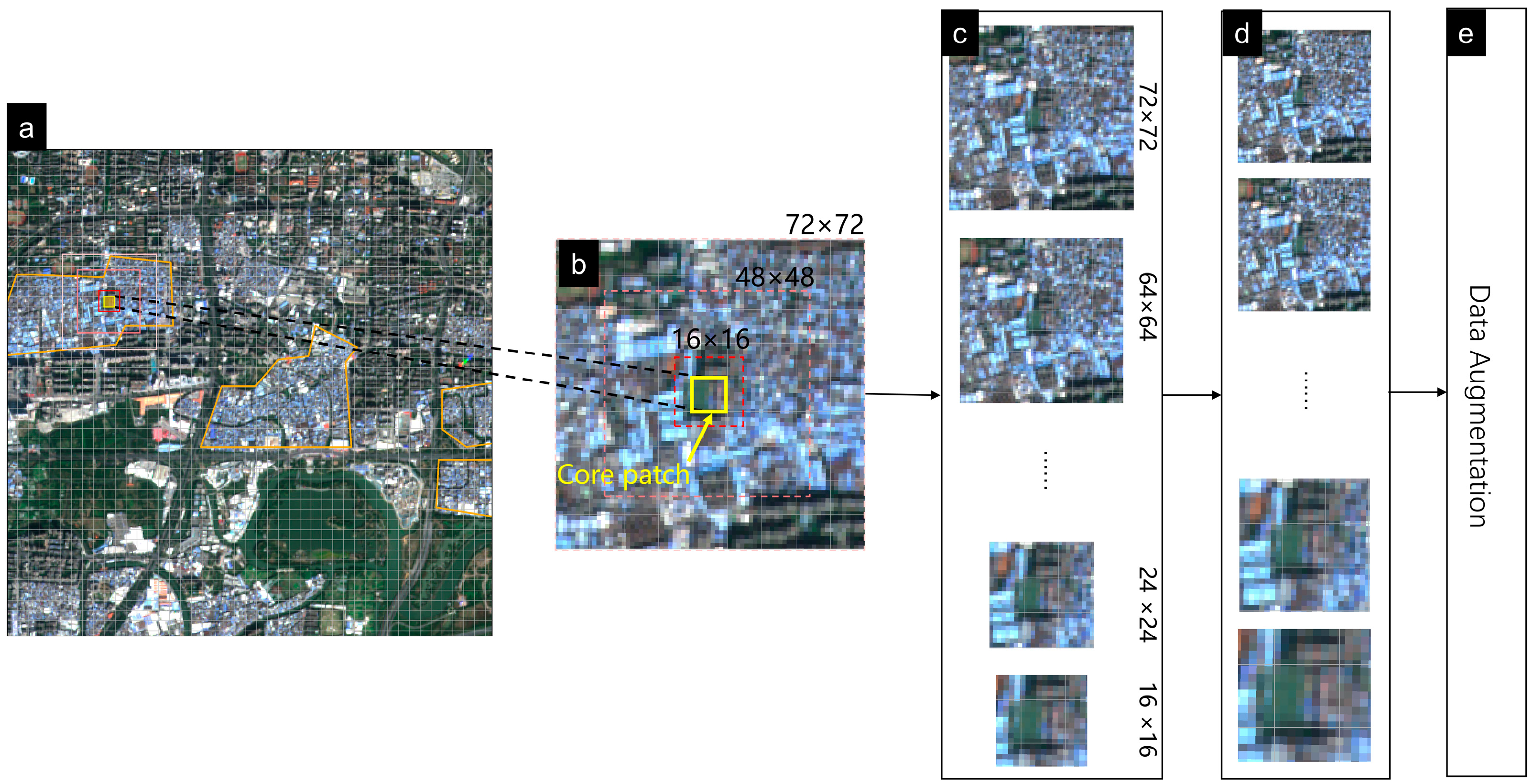
As an example, the steps of building sequential virtual scenes for training samples are shown in Figure 2. Irregular LCZ entities (Figure 2a) are first divided into 8 × 8 grids, then concentric enlarging virtual scenes (e.g., 16 × 16, …, 72 × 72) of each 8 × 8 patch are built (Figure 2b). Here, the size range of core patch and SVSs are referred to those used in previous studies [2,13,16]. Figure 2c clearly shows the context information of larger scenes can help us correctly identify the core patch as a building type, rather than a natural type as itself displays. Then, all patches in a sequence were resampled to 72 × 72 (Figure 2d) as input data to train the proposed model. Finally, the random data augmentation strategy, including mirroring, rotation, contrast enhancement, adding random noise, and so on (Figure 2e), is applied on the sequential patches to enlarge the sample set and then improve the model’s performance.
In the classification process, every 8 × 8 grid of an image and its virtual scenes are the inputs for the trained model. The type of the core patch is identified by not only its spectral information, but also the surrounding context information learned by the Bi-LSTM.

2.2. Image Patch Learning with ResNet

Deep convolutional neural networks (DCNN) are able to learn and express multilevel features from images autonomously and have been widely used in remote sensing classification. Generally, a DCNN is composed of multiple fully connected convolution layers and operations such as convolution summation, nonlinear bias, pooling, and others, which make it possible to understand the complex semantic information in image scenes. Among various DCNN models, ResNet has shown better performance in identifying complex LCZ entities than other models in several studies [17]. In this study, ResNet is used to learn the structure information of each virtual scene.
The basic unit of a ResNet is a residual block which generally consists of two or more convolutional layers and a shortcut connection. With the connection, the information from the previous residual block can be quickly transferred to the next residual one without any hindrance. Consequently, the information flow becomes fluent and the problems of gradient diminishment and degradation are remarkably alleviated. In addition, few additional parameter or calculation is needed when adding more shortcut connections to the network to construct a deep ResNet [21]. Therefore, the ResNet50 which includes 16 three-layer residual blocks is used in this study to learn as much knowledge from LCZ entities as possible.

2.3. Learning the Adjacent Relationship with Bi-LSTM

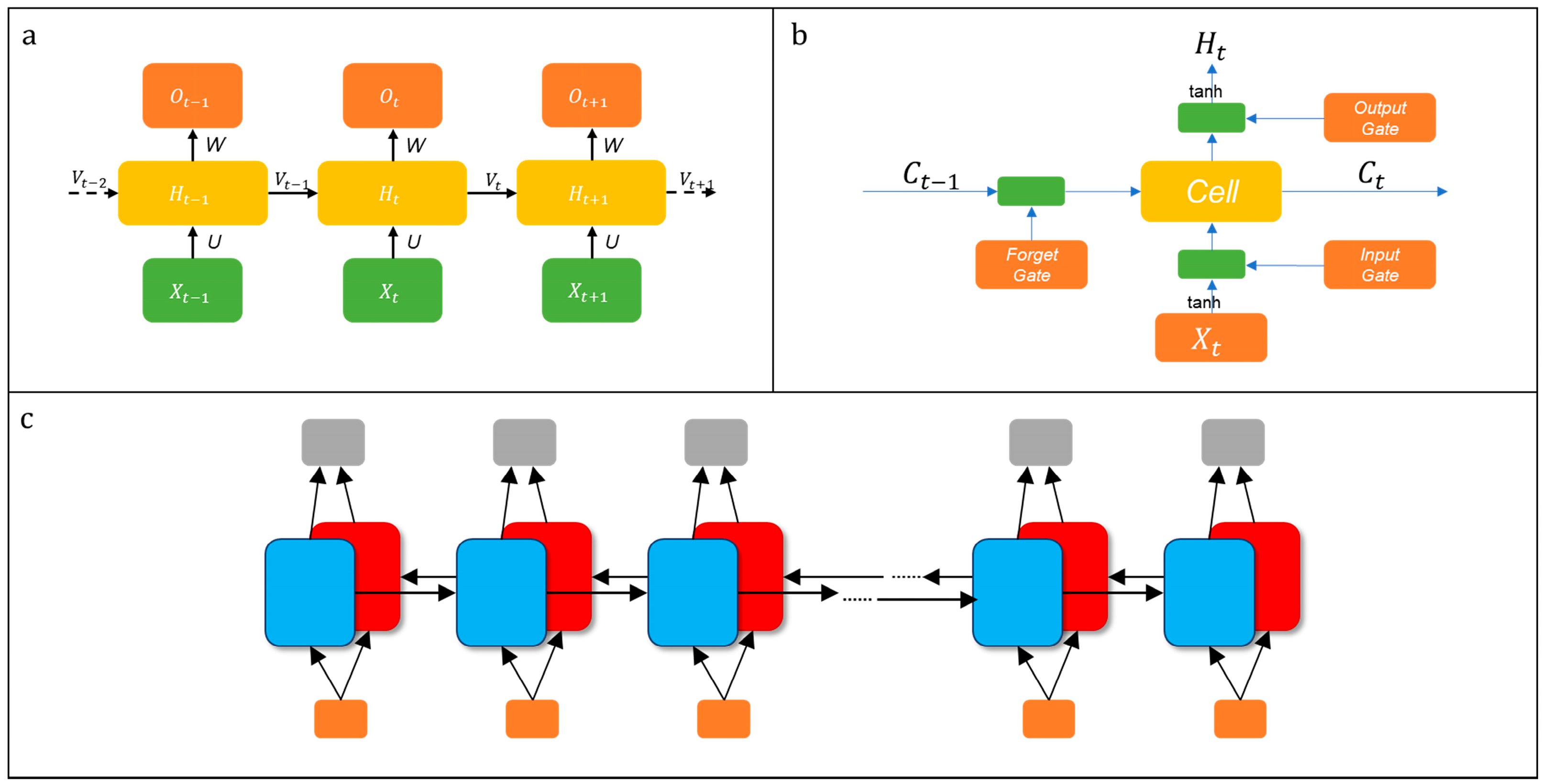
The Recurrent Neural Network (RNN) is designed to learn time series knowledge. In the model, each unit receives both the input data x (t) and the hidden state of previous unit h (t − 1), which is jointly determined by previous input x (t − 1) and an earlier hidden state h (t − 2). In addition, RNN units share the weight parameter matrix at each time step. With the distinctive structure, RNN can effectively extract temporal contextual information from unfixed length time series data, so that it has been widely used in natural language processing and time series image analysis. However, traditional RNNs are easy to suffer gradients vanishing or exploding in dealing with long-term sequences. A special RNN network, the long short-term memory networks (hereinafter referred to as LSTM), is adopted to solve the problem of short-term memory.
Different from the standard RNN network, a unit of LSTM is composed of one storage unit and three gates, namely the input gate, output gate, and forgetting gate, that decide which information should be added, output, and forgotten, respectively (Figure 3b). The special design allows LSTM to obtain better performance than traditional RNN in learning long time sequential data. With LSTM, Qiu et al. [13] extracted the seasonal characteristics of LCZ types from time series Sentinel-2 images for improving mapping accuracy. In another study [22], LSTM was successfully used to learn the spatial relationship between adjacent patches.
In the study, a bidirectional LSTM (hereinafter referred to as Bi-LSTM), which is composed of a forward LSTM and a backward LSTM, is constructed to learn the bidirectional adjacent relationship between sequential image patches. The number of Bi-LSTM units is equal to that of the sequential image patches (including the virtual scenes and the core patch). With this structure, the past and future contextual information of each image patch can be understood completely.

2.4. Weighting the Virtual Scenes with a Self-Attention Mechanism

Given that “mixed patches” are also easy to occur in virtual scenes, uncertainties may be introduced if the context information of all virtual scenes is equally considered in identifying the core patch. Here, a “self-attention” mechanism is developed to weight the contribution of a virtual scene according to the similarity between its intermediate hidden state and the final hidden state. With the method, those virtual scenes consisting of several types of LCZ are considered far away from the state of the whole sequence, and are then assigned a very small weight. In this way, the influence of “mixed patches” will be minimized, and the logical context will be enhanced to better support the classification of core patches.
In this study, the “self-attention” mechanism is considered as mapping a query and a set of key-value pairs to an output, where the query (Q), keys (K), values (V), and the output are all vectors [23] (Figure 4). The output is calculated as a weighted sum of the values, where the weight assigned to each value is calculated by a compatibility function of the query with the corresponding key. The idea can be described by the following equation:
Attention ( Q , K , V ) = softmax ( Q K T ) V
where the final hidden state H is thought as the Query and the intermediate hidden state h t obtained by Bi-LSTM of a virtual scene t is considered as the Key and Value. First, the similarity between h t and H is computed using the dot product, then the weight of the virtual scene can be figured out with the softmax function, as in Equation (2):
w t = exp ( e t ) t = 1 T exp ( e t ) , e t = ( H · h t T )
Then, the weighted sum c for the sequence virtual scenes of length T can be calculated out with the following equation [24]:
c = t = 1 T w t h t
where t = 1 T w t = 1 .

3. Test Sites and Data

3.1. Test Sites

In this study, four cities in the Pearl River Delta of China (PRD), Guangzhou, Shenzhen, Zhuhai, and Hong Kong, were selected for initializing and training the proposed SVS model. Four other global cities, i.e., New York, Vancouver, Tokyo, and Singapore, where LCZ reference labels are available, were selected as the validating sites. The images and selected samples of tests sites are shown in Figure 5.
The PRD is located in the south-central part of Guangdong Province, facing the South China Sea. As one of the China’s three greatest urban agglomerations, PRD is known for advanced manufacturing and modern service industries, innovation ability, and the great number of educated populations. In recent decades, PRD have experienced rapid urbanization, globalization, and industrialization. By the end of 2018, it had a permanent population of 70 million, a total GDP of 1.71 trillion dollars, and a per capita GDP of 24,500 USD. In the process of development, the Land Use Land Cover (LULC) of the natural and urban environment of PRD cities have witnessed a dramatic change in a short time due to their rapid urban expansion. By 2018, the average urbanization rate of the area had reached 84%. In this study, the four most known cities in PRD were selected as representatives for investigating the urban LCZ distribution in this area.
As shown in Figure 5e–h, the four validating cities have diverse urban landscape styles. Thus, tests on them are convincible for verifying the adaptability of the SVS model.

3.2. Sentinel Multispectral Imagery

In this study, Sentinel-2 images were used to map LCZ for the study sites with the proposed method. These images consist of 13 spectral bands, including visible bands and NIR bands with 10 m resolution, red edge bands and SWIR bands with 20 m resolution, and three other bands with 60 m resolution [25]. Because these data are the most detailed open access satellite imagery, it has been widely used in LCZ recognition [17]. Sentinel-2 images used for training and testing SVV models are freely accessed from Google Earth Engine (GEE dataset ID: ee.ImageCollection (“COPERNICUS/S2”)). The acquisition date and number of images are shown in Table 1.
For identifying LCZ, 10 bands with 10 m and 20 m resolutions were exploited, including the B2 (Blue), B3 (Green), B4 (Red), B8 (Near-infrared), B5 (Red Edge 1), B6 (Red Edge 2), B7 (Red Edge 3), B8 (Red Edge 4), B11 (Short-wavelength infrared 1), and B12 (Short-wavelength infrared 2), as the literature [2] suggested. The 20-m bands were resampled to 10 m with the cubic resampling algorithm. Other bands were not involved in this study, as previous work pointed out they contributed little to land cover classification and LCZ identification [17]. Image preprocessing stages, such as cropping, resampling, and cloud mask, were done on the Google Earth Engine platform [26].

3.3. Sample Preparation

The LCZ reference labels of the Tokyo, Singapore, Vancouver, and New York were taken from the LCZ Generator website https://lcz-generator.rub.de (accessed on 3 November 2022) [27]. For the four Chinese cities, we carefully delineated polygons of each LCZ type from the Sentinel-2 images with the help of the OpenStreetMap, to prepare the training and validating samples. In total, 1596 LCZ polygons were selected in total and some of them (as shown in Figure 5). We tried to find similar number of samples for each LCZ type; however, the sample sizes of different types still vary (as shown in Table 1). LCZ-G (water body) often has the greatest number of samples, while LCZ9, LCZ-B, and LCZ-C have much fewer samples. In view of this, the repeated upsampling strategy was used to expand the sample sets of some LCZ types whose number was much less than the average number. Finally, 5464 8 × 8 core patches were generated for Chinese cities, as shown in Table 2.

3.4. Accuracy Evaluation

The commonly used indicators for classification accuracy evaluation include: the Overall Accuracy (OA), Average Accuracy (AA), Kappa coefficient, producer’s Accuracy (precision), user’s Accuracy (recall), and F1_score. The first three are overall classification accuracy indicators, while the latter three are used for estimating the identification accuracy of a single category.
For imbalanced classification where the number of instances in each class highly varies, the Kappa coefficient is more suitable to assess the overall accuracy than the OA and AA. According to Equation (4), imbalanced confusion matrix will lead to a high P e and then a low kappa value. Namely, the uncertainty caused by imbalanced instances could be evaluated by the Kappa coefficient to some extent. Thus, the Kappa coefficient was employed as the main indicator of overall classification accuracy in this study. Besides, the harmonic average of Precision and Recall, the F1-score, was used to estimate the identification correctness of a single LCZ type. The formulas of these indicators are shown below:
k a p p a = P 0 P e 1 P e
P 0 = i = 1 t x i i N
P e = i = 1 t x i + x + i N 2
where x i i , x i + , x + i indicate the number of correctly classified samples, the number of reference samples, and the number of predicted samples, respectively, and N and t represent the total number of samples and the number of LCZ types, respectively.
F 1 s c o r e = 2 × p r e c i s i o n × r e c a l l p r e c i s i o n + r e c a l l
where:
P r e c i s i o n = T P T P + F P
R e c a l l = T P T P + F N
where T P , F P ,   F N indicate the correct, false, and missed detection of an LCZ type, respectively.

4. Results

Tests were conducted on the Ubuntu platform in a workstation with i7-9700K, 64G memory, and two Nvidia GTX2080super 8G GPU. Deep learning models were built based on the Pytorch framework, with the Adam optimizer [28] and Focal loss function [29]. The initial learning rate was set as 0.0001, which then exponentially decreased in the training process. All pre-train models were further trained through 1000 epoch sessions, while the LSTM pre-train model was finetuned 500 times.

4.1. Evaluating the Performance of the Proposed Method

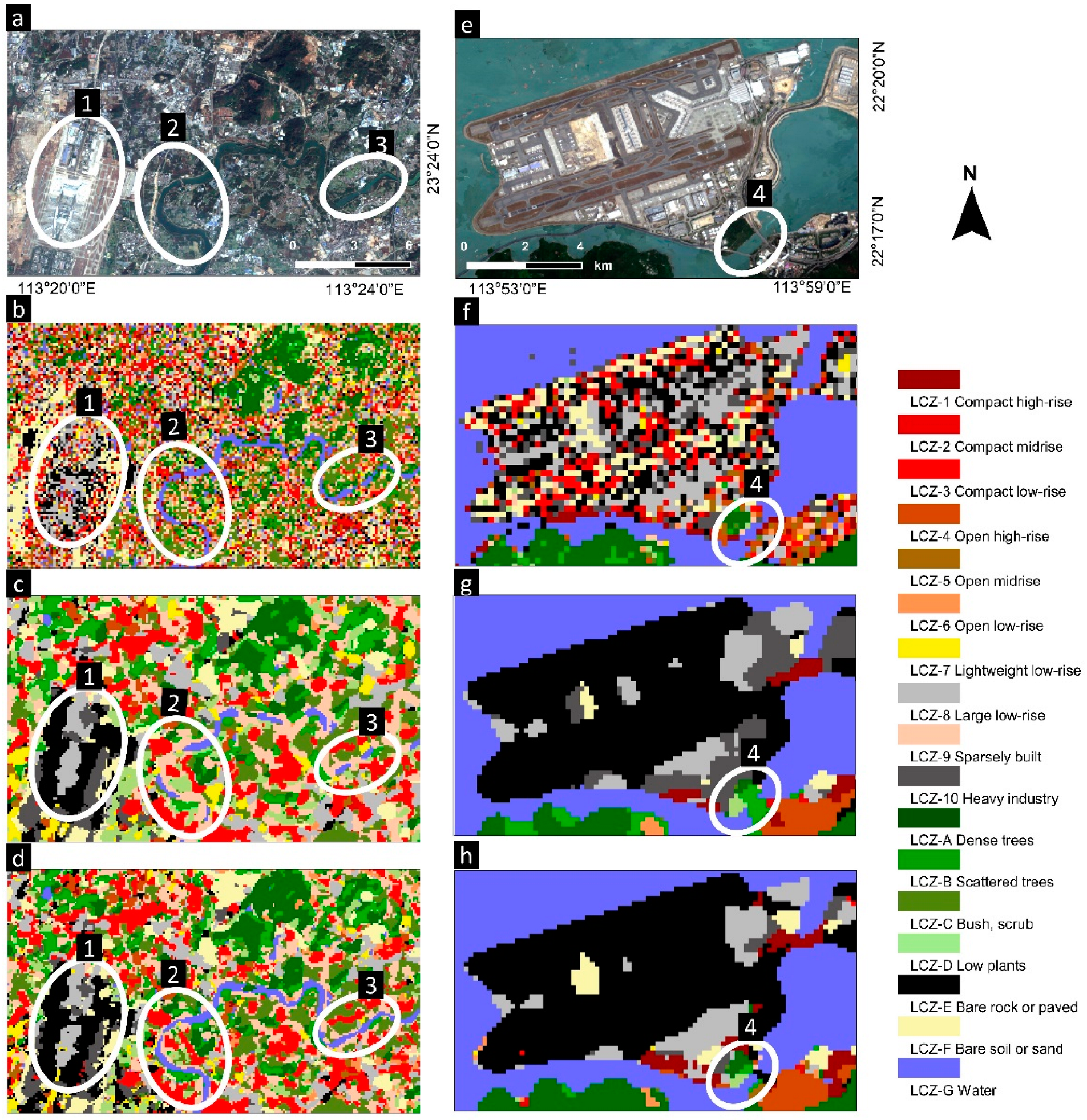
To evaluate its performance, the proposed method was tested in all eight cities, and compared with the GEE random forest and ResNet (input size 64 × 64). For the former, the number of trees and min leaf population were set as 100 and 1, respectively. Partial LCZ maps produced by them are shown in Figure 6 as examples to compare their performances. The classification accuracies of the three methods are shown in Figure 7 and Table 3.
In the Random Forest results (Figure 6b,f), pixels were classified just according to their spectral characteristics rather than the spatial connections and combinations. Given an LCZ building entity (e.g., LCZ 1-10) is often a spatial combination of multiple ground objects (e.g., buildings, grass, trees, or ponds), the pixel-based classifier was unable to identify LCZ entities completely and correctly. In the figure, all LCZ entities were divided into pixels of different types (e.g., the Baiyun Airport enclosed by ellipse 1). The serious classification errors impose adversely impacts on urban thermal environment analysis ultimately.
In the results of ResNet and SVS (Figure 6c,d,g,h), classes represented by pixels were barely seen and LCZ entities were almost completely identified (e.g., the runway and building area of the Baiyun Airport and Hong Kong Airport). Especially, it is found that some segments of the Pearl River were misclassified into LCZ-8 (marked by ellipse 2 and 3) in Figure 6c, and the road marked by ellipse 4 were misidentified as natural types due to the problem of mixed patches. This suggests small LCZ entities are probably ignored in scene classifications using large image patch.
Figure 6d,h indicate small entities, such as the Pearl River and road, which were correctly identified, suggesting the SVS was barely influenced by “mixed patches”. Especially the complete detection of the long and thin LCZ entity (e.g., the Pearl River) verifies that the spatial adjacent relationship between image patches could be effectively learned by the Bi-LSTM.
Figure 7 shows Random Forest classification achieved the lowest F1-scores for most LCZ types, especially those building types. That is because it is difficult to learn the spatial relationship among ground objects in high-resolution images. Note that the method obtained good performance in identifying LCZ-A, LCZ-F, and LCZ-G, suggesting it is still suitable for mapping types similar to traditional LULC.
Figure 7 shows ResNet classification using moderate patch attained the best F1-scores, while decreasing or increasing the patch size may lower the score. It implies the possibility that multiple types mixing in a larger image patch brought about remarkable uncertainty in LCZ identification. Comparatively, for types consisting of one object (e.g., LCZ-A, LCZ-F, and LCZ-G), the change of size had little impact on their F1-scores, as the problem of mixed patches did not exist. Figure 7 displays SVS classification obtained good F1-scores for all types. Overall, SVS got better performance than all ResNets (Table 2). Random Forest classification obtained the worst Kappa coefficient, OA, and AA; moreover, ResNet_56 had better performance than all other ResNets (Table 3).
The detailed results produced by ResNets with different sizes of image patches are shown in Figure 8, to display the influence of patch size on scene classification. As a comparison. In the figure, it is apparent that the size of mapped LCZ entities is closely related to the size of patches used in ResNet, rather than the actual size as shown in the image. When using small input size, the LCZ entities become fragmented, and similar to those produced by random forest. In results of ResNet with large input size, the LCZ entities become very large, while small objects are swallowed up, such as the island in panel (a) and segments of the Pear River in panel (b) and (c). Comparatively, in the SVS results, the size and shape of entities match the ground truth well. For instance, the island and river segments are correctly identified. The test shows the increase of patch size does not necessarily bring about performance improvement for scene classification. In addition, it verifies SVS outperforms scene classifiers with fixed size patch in identifying LCZ entities of diverse shapes and sizes.

4.2. The LCZ Maps of Test Cities

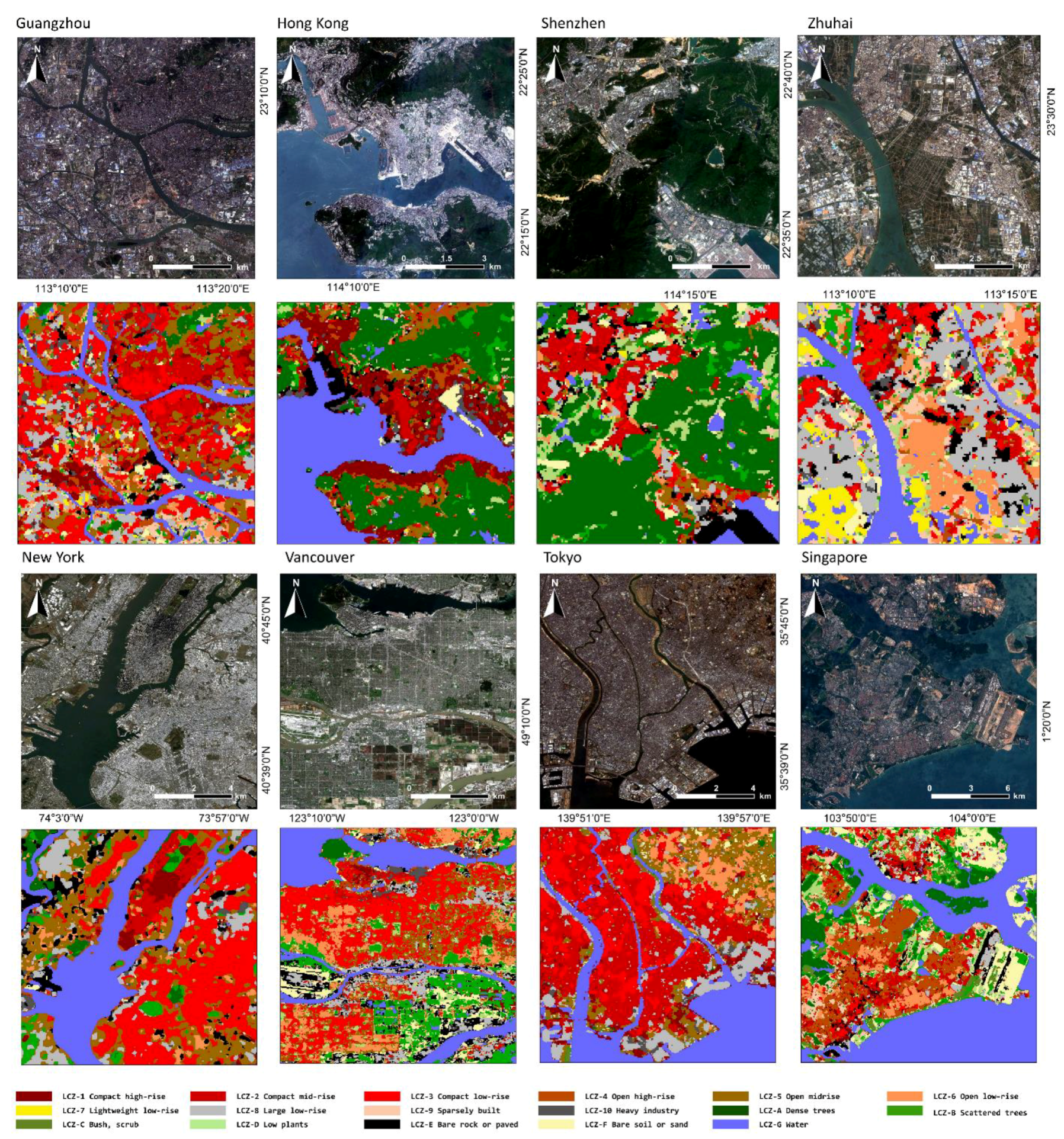
After verifying the validity of the proposed method, the LCZ maps of the eight test cities were produced and shown in Figure 9. Related classification accuracies for them are displayed in Table 4.
In Figure 9, it is observed that all LCZ maps match the reference images well, though each city has a distinctive LCZ composition and distribution. It proves the SVS can be used in cities of different landscape styles. Specifically, LCZ-1 or LCZ-2 are often seen in in Chinese cities, while LCZ-3 or LCZ-4 occupy most of New York, Vancouver, Tokyo, and Singapore.
In Table 4, the identification accuracy of a single LCZ type and overall accuracy for all types in test cities are displayed. The kappa coefficients in all cities are higher than 0.80, and five of them are even greater than 0.9, which verifies that the proposed methods can obtain good performance in cities of different tyles. In the table, most types achieve good F1-scores in test cities, except in several cases where very low F1-scores are observed. They were probably caused by the called “imbalanced classification”, where types having fewer samples are inclined to be misclassified in machine learning based classification. Given that it is common that some types do not exist or have very few instances in some cities, “imbalanced classification” should be carefully treated in LCZ mapping.

5. Discussions

5.1. The Influences of Sequence Compositions

We note that using a dense sequence of image patches in the proposed method would cost more time and computation resources than models using single size patches, though higher performance could be achieved. Thus, different sequence compositions were tested to evaluate the influences of compositions on LCZ mapping performance, and then examine whether using less patches could achieve similar accuracy. The compositions and results are shown in Table 5.
In Table 5, S1 is the original sequence for SVS, and S2 is the inverse sequence of S1. The test results show that S1 and S2 have the same accuracy, which indicates that the order of patch sequence does not affect the performance. That is because the Bi-LSTM is able to learn the spatial relationship bi-directionally. The table shows that when the sequence become sparse, the classification accuracy slightly decreases. The results suggest a dense sequence is necessary to obtain high performance, while the result of using a little sparser sequence is also acceptable when computation time or cost is concerned.

5.2. Weighting Virtual Scenes by the Self-Attention Mechanism

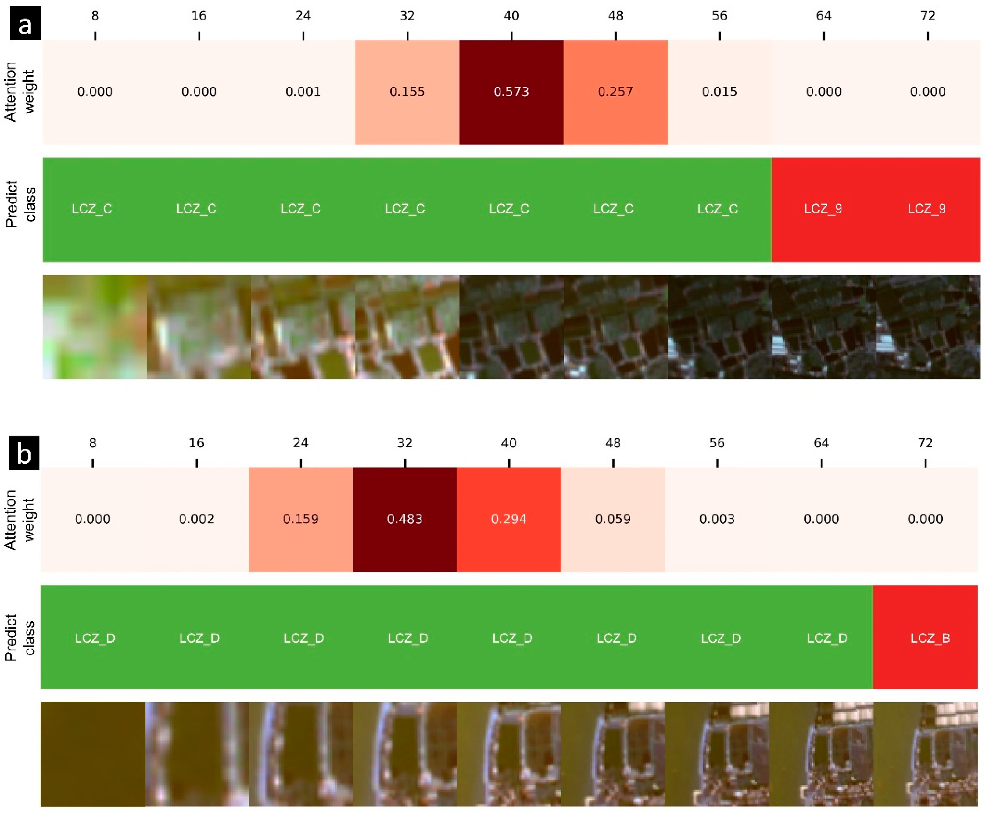
In order to reduce the misclassifications caused by “mixed patches” in lager scenes, the self-attention mechanism was used to weight virtual scenes according to their similarity to the whole sequence. Specifically, the weight process is illustrated in Figure 10.
It is seen that the core patch and most virtual scenes are identified as the same type, while greater scenes are often classed as other types, which become dominant in them. In the figure, moderately sized patches are assigned higher weights than small or large ones, which probably attributes to that the information of small patches is insufficient to support convincible classification, and large scenes often suffer from “mixed patches”. As the weight is calculated according to the similarity between current the virtual scene and the whole sequence, it is flexible and adaptable to the change of types or sites.
In Figure 11, the statistics of scenes’ weights for correctly identified samples are displayed. Generally, moderate virtual scenes are assigned higher weights than large scenes. The distribution histograms indicate that weight assignment is not fixed, but changes along with the vary of LCZ type, entity, and sites. This flexible assignment improves the accuracy and transferability of identifying irregular LCZ entities at different sites.

5.3. Contributions and Limitations of the Study

In the urban expansion megatrend, the sustainable development of the urban environment has attracted widespread attentions all over the world. LCZ mapping can support the monitoring and improving of the urban thermal environment and local climate, and thus, is of significance for climatologist, urban planners, and policy makers [10,11]. However, some urban areas are fuzzy in terms of LCZ entities [5], due to the non-quantitative, borderless description of LCZ types. For instance, it is hard to distinguish mid-rise and low-rise buildings strictly. In addition, the surface cover properties can be derived from earth observation data, which are limited and often affected by sunlight, season, etc., which results in the different understanding of surface parameters, and thus, affecting the understanding of LCZ entities. Consequently, deriving robust and high quality LCZ maps is still very difficult in local urban climate researches [18].
The WUDAPT uses the Random Forest to identify LCZ from Landsat images with manually collected training pixels [30]. Though it has been widely adopted in mapping LCZ in many sites [19], the method suffers from low resolution and strong noise, and does not adequately represent the spatial homogeneity of LCZs [1,2]. According to its definition, the identification of LCZs significantly depends on the context information. However, spectral characteristics of pixels rather than the spatial connections and combinations pixels are used to classify in Random Forest classification. Our studies also display that the Random Forest classification obtained very low accuracies in identifying LCZ building types, which consist of diverse objects and spatial relationship, as previous reported [1,2]. Thus, the pixel-based classification is not suitable for producing high-resolution LCZ maps.
Studies have reported that CNNs is able to learn the contextual features of LCZs, and achieve better accuracies than standard WUDAPT Random Forest classification [16]. The spatial context of the input image plays an important role in scene based LCZ mapping, while how to select the size of the input is still unclear. Different patch sizes have been tested to find the optimum one [2,13,16], and a larger image representation is suggested, as it can provide more contextual information for LCZ mapping compared to a smaller one [2]. However, the study discloses that the problem of “mixed patches” would increase when using larger patches. For an image patch consists of several partial LCZ types, it would be identified as the type who occupies the largest area in the scene classification. Meanwhile, the existences of types taking small area would be ignored. Tests with the commonly used model ResNet [16,17,21] indicate the size of produced LCZ entities is closely related to that of the input image, rather than their actual size. In the ResNet results, small LCZ entities such as rivers and islands are swallowed up by larger ones when using a large size (e.g., 64 × 64), which leads to both commission errors and omission errors. As the shapes and sizes of LCZ entities are always different, it is impossible to find an optimal fixed size for every entity.
In this study, the SVS is presented to map irregular LCZ entities with non-fixed image patches. In SVS, a very small “core patch” is used to scan irregular LCZ entities, and surrounding sequential virtual scenes are built to learn contextual features for the core patch with the help of Bi-LSTM. Besides, the ResNet and “self-attention” mechanism are used to learn the spatial structure of a virtual scene and weight the contribution of every virtual scene, respectively. The tests display that both small and large areas could be identified as homogeneous LCZ entities, especially thin rivers and tiny islands; thus, the non-fixed approach achieve better performance than Random Forest and ResNet using different sizes. Specifically, SVS classification obtained good accuracy on all natural and building types, while other classifiers just obtain good performance on a few of them. In the test, greater scene is often assigned very small weights, as its hidden states is different from the whole sequence. This discloses that greater scene has a higher chance to suffer the problem of “mixed patches”, i.e., that more than one LCZ entities emerge there. Comparatively, moderate size scenes are often assigned higher weights, as they have more contextual information than small ones, and are less contaminated by other LCZ types.
Figure 10 and Figure 11 disclose the virtual scenes given higher weights are not fixed, but change along with the variance of LCZ entities. The flexibility of weights assignment could improve the accuracy and adaptability of identifying irregular LCZ entities at different sites. In order to test the transferability of the SVS model, we applied it to various cities all over the world, including the Pearl River Delta of China, New York, Vancouver, Tokyo, and Singapore. Those cities have diverse urban landscape styles, e.g., different LCZ composition and distribution. Experiments indicate the model achieves very good performance (kappa coefficients are about 0.90) at all sites. Tests proved SVS model can deal with cities of different styles successfully.
One evident limitation of the method is that more time and computation resources are probably needed than conventional models, as a dense sequence of image patches and their spatial relationship should be built and learned in the process. The test with different compositions discloses when the sequence become sparser, the classification accuracy slightly decreases. Thus, a little sparser sequence could be suggested when computation time or cost is concerned. Another one should be noted is the problem of “imbalanced classification”, which is also the common problem in machine learning-based classification. Given that it is common that some LCZ types have very few instances while others possess much more, a new sampling technique and cost matrix should be involved in the future to reduce the adverse impacts of imbalanced classification.

6. Conclusions

In this study, a sequential virtual scene-based method is presented for accurately identifying irregular LCZ entities, which includes a small initial “core patch” for scanning every part of irregular LCZ entities, and sequential virtual scenes (SVS) for proving abundant contextual information to help identify the core patch. Specifically, a Bi-LSTM and “self-attention” mechanism were employed, respectively to learn the adjacent spatial relationship between scenes and weight the contribution of scenes. Comparison experiments suggest SVS achieves better accuracies than both random forest and ResNet, especially in irregular LCZ entities of diverse shapes and sizes. Tests in cities of different styles indicate it is a promising way to carry out large scale LCZ mapping because of its flexibility and adaptability. Further investigation reveals using sparser sequence in the model is also acceptable when computation time or cost is concerned, though a dense sequence is necessary to obtain high performance. In the future work, we will focus on how to optimize the composition of sequential scenes for improving the model’s efficiency.

Author Contributions

Conceptualization, Q.Y. and C.Z.; methodology, Q.Y.; software, Q.Y.; writing—original draft preparation, Q.Y., H.G.; writing—review and editing, P.G., H.L. and C.Z.; supervision, C.Z.; project administration, C.Z. All authors have read and agreed to the published version of the manuscript.

Funding

This study was sponsored by the Open Fund of Key Laboratory of Urban Land Resources Monitoring and Simulation, Ministry of Natural Resources(KF- 2020-05-007), the science and technology innovation project of Yunnan Bureau of Geology and Minerals Exploration and Development (No. 202235), the key research and development program of Hubei province (No. 2021BID009), the fine investigation and risk assessment of geological hazards in critical regions of Yunnan Province of 2020 (No. YNLH202011010793/A), the Natural Science Foundation of China (No. 41772352), the Open Fund of Badong National Observation and Research Station of Geohazards (No. BNORSG-202104).

Institutional Review Board Statement

Not applicable.

Informed Consent Statement

Not applicable.

Data Availability Statement

Not applicable.

Conflicts of Interest

The authors declare no conflict of interest.

References

  1. Yoo, C.; Han, D.; Im, J.; Bechtel, B. Comparison between Convolutional Neural Networks and Random Forest for Local Climate Zone Classification in Mega Urban Areas Using Landsat Images. ISPRS J. Photogramm. Remote Sens. 2019, 157, 155–170. [Google Scholar] [CrossRef]
  2. Liu, S.; Shi, Q. Local Climate Zone Mapping as Remote Sensing Scene Classification Using Deep Learning: A Case Study of Metropolitan China. ISPRS J. Photogramm. Remote Sens. 2020, 164, 229–242. [Google Scholar] [CrossRef]
  3. Cai, M.; Ren, C.; Xu, Y.; Lau, K.K.-L.; Wang, R. Investigating the Relationship between Local Climate Zone and Land Surface Temperature Using an Improved WUDAPT Methodology—A Case Study of Yangtze River Delta, China. Urban Clim. 2018, 24, 485–502. [Google Scholar] [CrossRef]
  4. Pachauri, R.K.; Mayer, L.; Intergovernmental Panel on Climate Change (Eds.) Climate Change 2014: Synthesis Report; Intergovernmental Panel on Climate Change: Geneva, Switzerland, 2015; ISBN 978-92-9169-143-2.
  5. Bechtel, B.; Daneke, C. Classification of Local Climate Zones Based on Multiple Earth Observation Data. IEEE J. Sel. Top. Appl. Earth Obs. Remote Sens. 2012, 5, 1191–1202. [Google Scholar] [CrossRef]
  6. Coseo, P.; Larsen, L. How Factors of Land Use/Land Cover, Building Configuration, and Adjacent Heat Sources and Sinks Explain Urban Heat Islands in Chicago. Landsc. Urban Plan. 2014, 125, 117–129. [Google Scholar] [CrossRef]
  7. Tuia, D.; Moser, G.; Le Saux, B.; Bechtel, B.; See, L. 2017 IEEE GRSS Data Fusion Contest: Open Data for Global Multimodal Land Use Classification [Technical Committees]. IEEE Geosci. Remote Sens. Mag. 2017, 5, 70–73. [Google Scholar] [CrossRef]
  8. Guo, G.; Wu, Z.; Xiao, R.; Chen, Y.; Liu, X.; Zhang, X. Impacts of Urban Biophysical Composition on Land Surface Temperature in Urban Heat Island Clusters. Landsc. Urban Plan. 2015, 135, 1–10. [Google Scholar] [CrossRef]
  9. Fu, C.; Song, X.-P.; Stewart, K. Integrating Activity-Based Geographic Information and Long-Term Remote Sensing to Characterize Urban Land Use Change. Remote Sens. 2019, 11, 2965. [Google Scholar] [CrossRef] [Green Version]
  10. Stewart, I.D.; Oke, T.R. Local Climate Zones for Urban Temperature Studies. Bull. Am. Meteorol. Soc. 2012, 93, 1879–1900. [Google Scholar] [CrossRef]
  11. Bechtel, B.; Demuzere, M.; Mills, G.; Zhan, W.; Sismanidis, P.; Small, C.; Voogt, J. SUHI Analysis Using Local Climate Zones—A Comparison of 50 Cities. Urban Clim. 2019, 28, 100451. [Google Scholar] [CrossRef]
  12. Ching, J.; Mills, G.; Bechtel, B.; See, L.; Feddema, J.; Wang, X.; Ren, C.; Brousse, O.; Martilli, A.; Neophytou, M.; et al. WUDAPT: An Urban Weather, Climate, and Environmental Modeling Infrastructure for the Anthropocene. Bull. Am. Meteorol. Soc. 2018, 99, 1907–1924. [Google Scholar] [CrossRef] [Green Version]
  13. Qiu, C.; Mou, L.; Schmitt, M.; Zhu, X.X. Local Climate Zone-Based Urban Land Cover Classification from Multi-Seasonal Sentinel-2 Images with a Recurrent Residual Network. ISPRS J. Photogramm. Remote Sens. 2019, 154, 151–162. [Google Scholar] [CrossRef] [PubMed]
  14. Keyport, R.N.; Oommen, T.; Martha, T.R.; Sajinkumar, K.S.; Gierke, J.S. A Comparative Analysis of Pixel- and Object-Based Detection of Landslides from Very High-Resolution Images. Int. J. Appl. Earth Obs. Geoinf. 2018, 64, 1–11. [Google Scholar] [CrossRef]
  15. Simanjuntak, R.M.; Kuffer, M.; Reckien, D. Object-Based Image Analysis to Map Local Climate Zones: The Case of Bandung, Indonesia. Appl. Geogr. 2019, 106, 108–121. [Google Scholar] [CrossRef]
  16. Rosentreter, J.; Hagensieker, R.; Waske, B. Towards Large-Scale Mapping of Local Climate Zones Using Multitemporal Sentinel 2 Data and Convolutional Neural Networks. Remote Sens. Environ. 2020, 237, 111472. [Google Scholar] [CrossRef]
  17. Qiu, C.; Schmitt, M.; Mou, L.; Ghamisi, P.; Zhu, X.X. Feature Importance Analysis for Local Climate Zone Classification Using a Residual Convolutional Neural Network with Multi-Source Datasets. Remote Sens. 2018, 10, 1572. [Google Scholar] [CrossRef] [Green Version]
  18. Qiu, C.; Tong, X.; Schmitt, M.; Bechtel, B.; Zhu, X.X. Multilevel Feature Fusion-Based CNN for Local Climate Zone Classification From Sentinel-2 Images: Benchmark Results on the So2Sat LCZ42 Dataset. IEEE J. Sel. Top. Appl. Earth Obs. Remote Sens. 2020, 13, 2793–2806. [Google Scholar] [CrossRef]
  19. Bechtel, B.; Alexander, P.; Böhner, J.; Ching, J.; Conrad, O.; Feddema, J.; Mills, G.; See, L.; Stewart, I. Mapping Local Climate Zones for a Worldwide Database of the Form and Function of Cities. ISPRS Int. J. Geo-Inf. 2015, 4, 199–219. [Google Scholar] [CrossRef] [Green Version]
  20. Verdonck, M.-L.; Okujeni, A.; van der Linden, S.; Demuzere, M.; De Wulf, R.; Van Coillie, F. Influence of Neighbourhood Information on ‘Local Climate Zone’ Mapping in Heterogeneous Cities. Int. J. Appl. Earth Obs. Geoinf. 2017, 62, 102–113. [Google Scholar] [CrossRef]
  21. He, K.; Zhang, X.; Ren, S.; Sun, J. Deep Residual Learning for Image Recognition. arXiv 2015, arXiv:1512.03385. [Google Scholar]
  22. Ma, A.; Filippi, A.; Wang, Z.; Yin, Z. Hyperspectral Image Classification Using Similarity Measurements-Based Deep Recurrent Neural Networks. Remote Sens. 2019, 11, 194. [Google Scholar] [CrossRef]
  23. Vaswani, A.; Shazeer, N.; Parmar, N.; Uszkoreit, J.; Jones, L.; Gomez, A.N.; Kaiser, L.; Polosukhin, I. Attention Is All You Need. In Proceedings of the Advances in Neural Information Processing Systems, Long Beach, CA, USA, 4–9 December 2017. [Google Scholar]
  24. Bahdanau, D.; Cho, K.; Bengio, Y. Neural Machine Translation by Jointly Learning to Align and Translate. arXiv 2016, arXiv:1409.0473. [Google Scholar]
  25. Drusch, M.; Del Bello, U.; Carlier, S.; Colin, O.; Fernandez, V.; Gascon, F.; Hoersch, B.; Isola, C.; Laberinti, P.; Martimort, P.; et al. Sentinel-2: ESA’s Optical High-Resolution Mission for GMES Operational Services. Remote Sens. Environ. 2012, 120, 25–36. [Google Scholar] [CrossRef]
  26. Gorelick, N.; Hancher, M.; Dixon, M.; Ilyushchenko, S.; Thau, D.; Moore, R. Google Earth Engine: Planetary-Scale Geospatial Analysis for Everyone. Remote Sens. Environ. 2017, 202, 18–27. [Google Scholar] [CrossRef]
  27. Demuzere, M.; Kittner, J.; Bechtel, B. LCZ Generator: A Web Application to Create Local Climate Zone Maps. Front. Environ. Sci. 2021, 9, 637455. [Google Scholar] [CrossRef]
  28. Kingma, D.P.; Ba, J. Adam: A Method for Stochastic Optimization. arXiv 2017, arXiv:1412.6980. [Google Scholar]
  29. Lin, T.-Y.; Goyal, P.; Girshick, R.; He, K.; Dollár, P. Focal Loss for Dense Object Detection. arXiv 2018, arXiv:1708.02002. [Google Scholar]
  30. Hay Chung, L.C.; Xie, J.; Ren, C. Improved machine-learning mapping of local climate zones in metropolitan areas using composite Earth observation data in Google Earth Engine. Build. Environ. 2021, 199, 107879. [Google Scholar] [CrossRef]
Figure 1. The framework of concentric sequential virtual scenes (SVS).
Remotesensing 14 05564 g001
Figure 2. The steps of building sequential virtual scenes (SVS) for samples (ae).
Remotesensing 14 05564 g002
Figure 3. The structure of RNN and LSTM. (a) Simple-RNN; (b) LSTM unit; and (c) Bidirectional LSTM.
Remotesensing 14 05564 g003
Figure 4. The self-attention mechanism.
Remotesensing 14 05564 g004
Figure 5. The test sites. (ad) Images and training samples in Guangzhou, Shenzhen, Hong Kong, and Zhuhai, respectively; (eh) Images and validation samples in New York, Vancouver, Tokyo, and Singapore, respectively.
Remotesensing 14 05564 g005
Figure 6. The partial results of three methods. (ad) The LCZ maps around the Guangzhou Baiyun Airport: (a) original image, (b) Random Forest result, (c) ResNet result, and (d) SVS result. (eh) LCZ maps of the Hongkong international Airport: (e) original image, (f) Random Forest result, (g) ResNet result, and (h) SVS result.
Remotesensing 14 05564 g006
Figure 7. The identification accuracy of Random Forest, ResNet, and SVS, for each LCZ type. Here, different patch sizes were tested to check whether patch size matters to traditional scene classifier, e.g., ResNet_16 means the model uses a 16 × 16 patch size.
Remotesensing 14 05564 g007
Figure 8. The samples produced by different ResNets and the SVS. (a) An island in Pear River, (b) and (c) different segments of Pear River.
Remotesensing 14 05564 g008
Figure 9. The LCZ maps of test cities. Here, the first and third rows display the original images, and the second and fourth image rows illustrate corresponding LCZ maps.
Remotesensing 14 05564 g009
Figure 10. Samples of weighting sequential scenes. (a) LCZ-C and (b) LCZ-D. In each panel, from the first to the fourth row, they indicate the size, weight, type, and the original image of the patch, respectively.
Remotesensing 14 05564 g010
Figure 11. The statistics of scenes’ weights for correctly identified samples. Here, the color indicates the size of patch.
Remotesensing 14 05564 g011
Table 1. The acquisition date and number of Sentinel-2 image.
CityGuangzhouHong KongShenzhenZhuhaiTokyoSingaporeVancouverNew York
Date15 March 202112 March 202112 March 202115 March 20213 March 202125 April 202111 March 20213 March 2021
20 March 202115 March 202115 March 202120 March 202118 March 2021 29 March 20218 March 2021
25 March 202117 March 202117 March 20214 April 202123 March 2021 31 March 202111 March 2021
29 April 202120 March 202120 March 202124 April 20217 April 2021 5 April 202113 March 2021
25 March 202125 March 20214 May 202122 April 2021 13 April 202121 March 2021
27 March 202127 March 20219 May 202127 April 2021 15 April 20215 April 2021
11 April 202111 April 202114 May 2021 18 April 202120 April 2021
21 April 202121 April 2021 20 April 202112 May 2021
29 April 202129 April 2021 13 May 202115 May 2021
11 May 202111 May 2021 17 May 2021
16 May 202116 May 2021 27 May 2021
Total41111761911
Table 2. The numbers of core patch samples for each LCZ type.
ClassGuangzhouHong KongShenzhenZhuhaiTokyoSingaporeVancouverNew YorkTotal
TrainTestTrainTestTrainTestTrainTestTrainTestTrainTestTrainTestTrainTest
LCZ-11918124772533312649222813411810747678
LCZ-2221028296959161246201687319912755762
LCZ-32841433984611047231773430146528679
LCZ-41741522319224551/248107231063667
LCZ-515212511221732173515241127122310317
LCZ-6331291124262721221020790532353576
LCZ-76798984161////149
LCZ-8726125722166842683019383129566730969
LCZ-91412671894013/12353//295
LCZ-103641191535391617136/4018209324
LCZ-A374246621212372307031597257208901151702
LCZ-B98215798728123241391687232822
LCZ-C56647032322714619785//484
LCZ-D106342221141214/15065178/373
LCZ-E64374889112781612/6428156687432878
LCZ-F192339137417650107154662621134419941172
LCZ-G114331201249271120199622279868329362526860263827
Total52071773567192768576662379834733451444577255158068514,675
“/” indicates there is no such type in the city.
Table 3. The overall accuracy of different methods.
ModelKappa × 100OA (%)AA (%)
ResNet_1672.7176.1166.53
ResNet_2475.978.8771.82
ResNet_3278.6381.374.89
ResNet_4080.3182.7577.35
ResNet_4881.4983.7680.8
ResNet_5683.1985.2681.85
ResNet_6482.584.6681.37
ResNet_7282.7784.9280.92
Random Forest58.7164.0447.85
SVS85.9687.7282.06
Table 4. The F1-score and Kappa coefficient of LCZ types in test cities.
ClassGuangzhouHong KongShenzhenZhuhaiTokyoSingaporeVancouverNew York
F1-Score
(%)
LCZ-185.00 86.30 82.14 94.74 100.00 42.86 97.87 100.00
LCZ-266.67 58.14 86.89 70.00 62.65 77.46 80.00 100.00
LCZ-3100.00 95.00 100.00 96.04 84.87 88.89 86.96 96.77
LCZ-4100.00 77.27 72.22 86.27 /82.05 75.00 /
LCZ-586.96 53.85 68.42 70.00 94.89 /91.67 80.00
LCZ-676.92 62.50 78.79 70.00 75.25 90.26 100.00 /
LCZ-787.50 100.00 57.14 100.00 ////
LCZ-888.71 26.32 64.86 90.48 94.57 86.86 90.76 96.55
LCZ-991.67 100.00 36.36 63.16 /92.50 //
LCZ-10100.00 82.35 87.50 100.00 97.01 /95.45 100.00
LCZ-A100.00 98.04 93.62 100.00 100.00 96.12 100.00 80.00
LCZ-B87.50 23.53 52.63 42.86 82.71 88.49 99.25 /
LCZ-C26.67 66.67 72.94 89.29 76.29 94.96 //
LCZ-D50.00 95.24 60.00 72.73 /97.40 88.89 /
LCZ-E83.33 97.40 79.50 22.22 /82.35 94.74 94.92
LCZ-F100.00 62.50 85.80 89.52 100.00 93.90 94.74 100.00
LCZ-G99.70 100.00 99.58 100.00 99.61 99.83 99.82 99.10
Kappa91.3891.38 83.98 81.37 86.42 90.20 90.50 96.62
“/” indicates that there is no such type in the city.
Table 5. The tests with different sequence compositions.
NameSequence CompositionKappa × 100OA (%)AA (%)
S1(*,16,24,32,40,48,56,64,72)85.9687.7182.06
S2(72,64,56,48,40,32,24,16,8)85.8587.6182.77
S3(24,32,40,48,56)84.5286.4683.38
S4(24,40,56)83.3385.4181.65
S5(56)82.1983.2580.85
* Indicates the size of image patch.
Publisher’s Note: MDPI stays neutral with regard to jurisdictional claims in published maps and institutional affiliations.