Article

DUPnet: Water Body Segmentation with Dense Block and Multi-Scale Spatial Pyramid Pooling for Remote Sensing Images

1
School of Aerospace Science and Technology, Xidian University, Xi’an 710026, China
2
Department of Aerospace and Geodesy, Data Science in Earth Observation, Technical University of Munich (TUM), 80333 Munich, Germany
*
Author to whom correspondence should be addressed.
These authors contributed equally to this work.
Remote Sens. 2022, 14(21), 5567; https://doi.org/10.3390/rs14215567
Submission received: 16 September 2022 / Revised: 2 November 2022 / Accepted: 3 November 2022 / Published: 4 November 2022
(This article belongs to the Special Issue Deep Learning for Satellite Image Segmentation)

Abstract

:
Water body segmentation is an important tool for the hydrological monitoring of the Earth. With the rapid development of convolutional neural networks, semantic segmentation techniques have been used on remote sensing images to extract water bodies. However, some difficulties need to be overcome to achieve good results in water body segmentation, such as complex background, huge scale, water connectivity, and rough edges. In this study, a water body segmentation model (DUPnet) with dense connectivity and multi-scale pyramidal pools is proposed to rapidly and accurately extract water bodies from Gaofen satellite and Landsat 8 OLI (Operational Land Imager) images. The proposed method includes three parts: (1) a multi-scale spatial pyramid pooling module (MSPP) is introduced to combine shallow and deep features for small water bodies and to compensate for the feature loss caused by the sampling process; (2) dense blocks are used to extract more spatial features to DUPnet’s backbone, increasing feature propagation and reuse; (3) a regression loss function is proposed to train the network to deal with the unbalanced dataset caused by small water bodies. The experimental results show that the F1, MIoU, and FWIoU of DUPnet on the 2020 Gaofen dataset are 97.67%, 88.17%, and 93.52%, respectively, and on the Landsat River dataset, they are 96.52%, 84.72%, 91.77%, respectively.

1. Introduction

Due to the advantages of large coverage, low cost, and short data acquisition period, remote sensing has been widely used in water body segmentation [1,2,3]. Water body segmentation is important for water resource management, ecological evaluation, and environmental protection [4,5]. The key to water body segmentation is to highlight the features of water bodies from complex backgrounds.
Traditional water body segmentation algorithms are used to extract water bodies directly by calculating a certain water body index, such as Normalized Difference Water Index (NDWI) [6] and Modified Normalized Difference Water Index (MNDWI) [7], and then by setting the corresponding thresholds. The water body index segmentation algorithm relies on thresholds that are set manually. The main aim of these indexes is to exploit the differences in the reflectance of water bodies at different wavelengths and to enhance the information about water bodies [8]. However, due to the diversity and complexity of the background, the different thresholds need to be adjusted for different scenarios. Machine learning-based water body segmentation algorithms build a relationship between water body samples and masks, which reduces the reliance on segmentation thresholds. Many popular algorithms such as Support Vector Machine (SVM) [9], Random Forests (RF) [10], Decision Tree (DT), and Deep Learning (DL) have been developed in remote sensing image segmentation [11,12]. DL has attracted more attention in image segmentation mainly due to its strong ability to extract variables to express feature information [13], which boosts the intelligent and automatic interpretation of remote sensing images.
With the rapid development of deep learning, Ronneberger et al. [14] proposed the U-Net model for medical image segmentation in 2015. U-Net is a symmetric structure and one of the first techniques to use encoder–decoder networks for semantic segmentation. U-Net achieves relatively high accuracy using only a small amount of training data. The encoder module is used to categorize and analyze the low-level local pixel values of the image and obtain higher-order semantic information, while the decoder module is to collect the semantic information and gradually recovers the spatial information of the features.
The encoder–decoder network employs an organized recurrent neural network to deal with the sequence-to-sequence prediction problem, which has been successfully applied to a wide variety of computer vision tasks [14,15], and remote sensing image semantic segmentation [16]. In 2020, He et al. [17] proposed an improved U-Net network model to extract water bodies on Gaofen-2 remote sensing images and made the feature map as the input of conditional random field (CRF) to improve the fineness of target object edge segmentation. Although the model has a good effect, there is still a need to improve the extraction effect in areas where surrounding conditions differ greatly from the study area. Other networks for image segmentation have also been proposed, such as FCN [18], SegNet [19], RefineNet [20], PSPNet [21], Deeplab series [15,22,23], etc. The Deeplab series and PSPNet use inflated convolutions, which increase the input size without pooling layers, resulting in a wider range of information in the output for each convolution [24]. Other semantic segmentation networks are also proposed in water body segmentation research. These networks include HRNet V2 [25], which is utilized to enhance the high-resolution representation by pooling all parallel convolutional representations; the WatNet [16], which is used for surface water mapping; and PSPNet, which is applied to detect the water shoreline [26].
Although these DL methods greatly improved the accuracy and efficiency of water body extraction, there are still challenges in the water body extraction: (1) in the deep learning forward propagation, the resolution of feature maps is reduced due to the repeated max-pooling layers, which leads to the loss of detailed water body information; (2) as the receptive fields of pixels vary, the feature maps produced by convolutional layers at varying depths contain feature information at varying sizes. The integration of gathered features at different scales deserves further research to improve the accuracy of water body extraction.
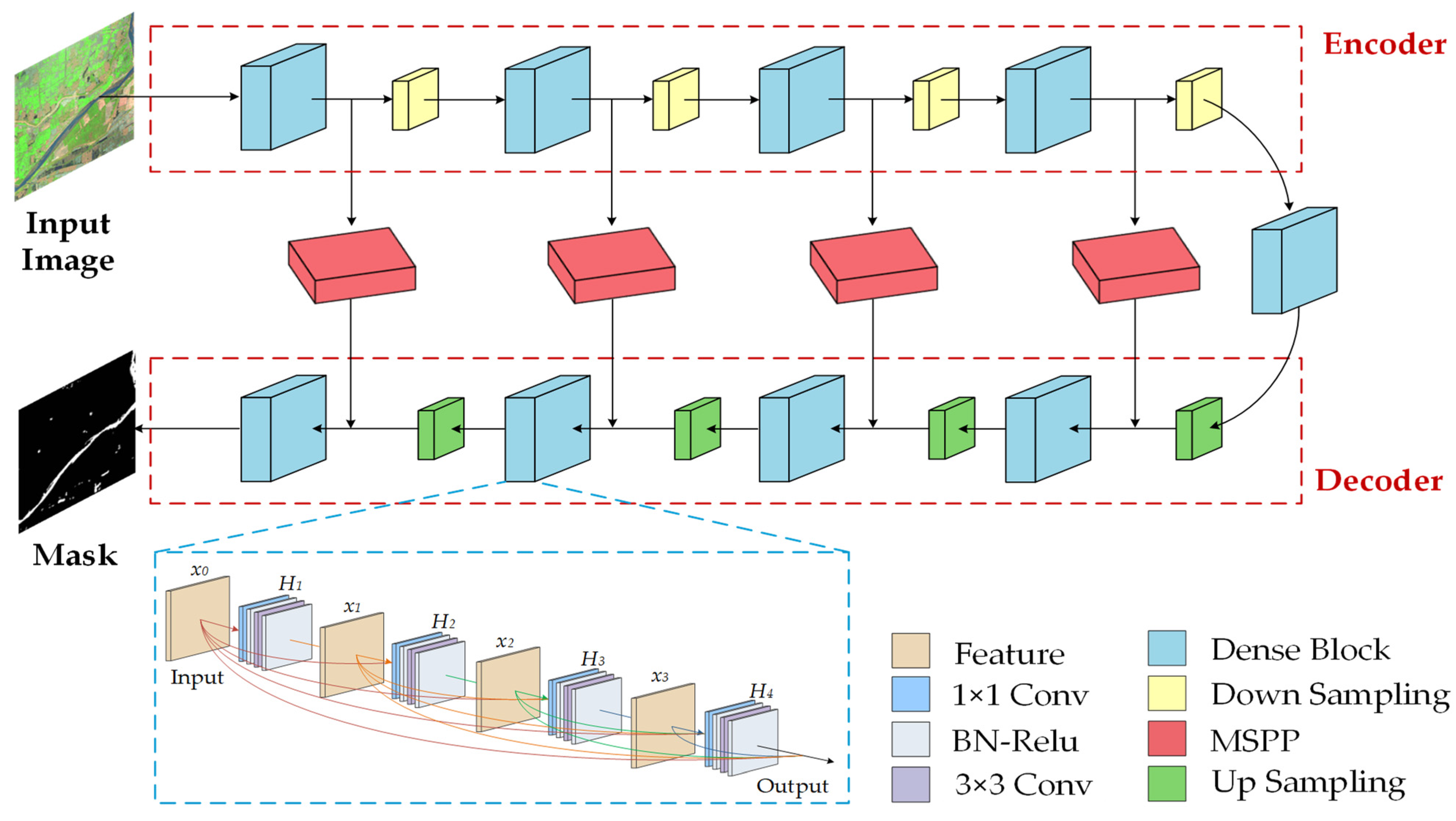
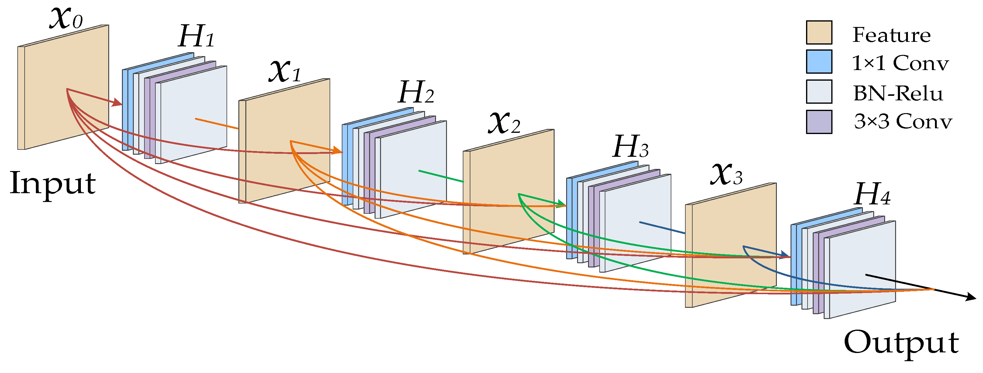
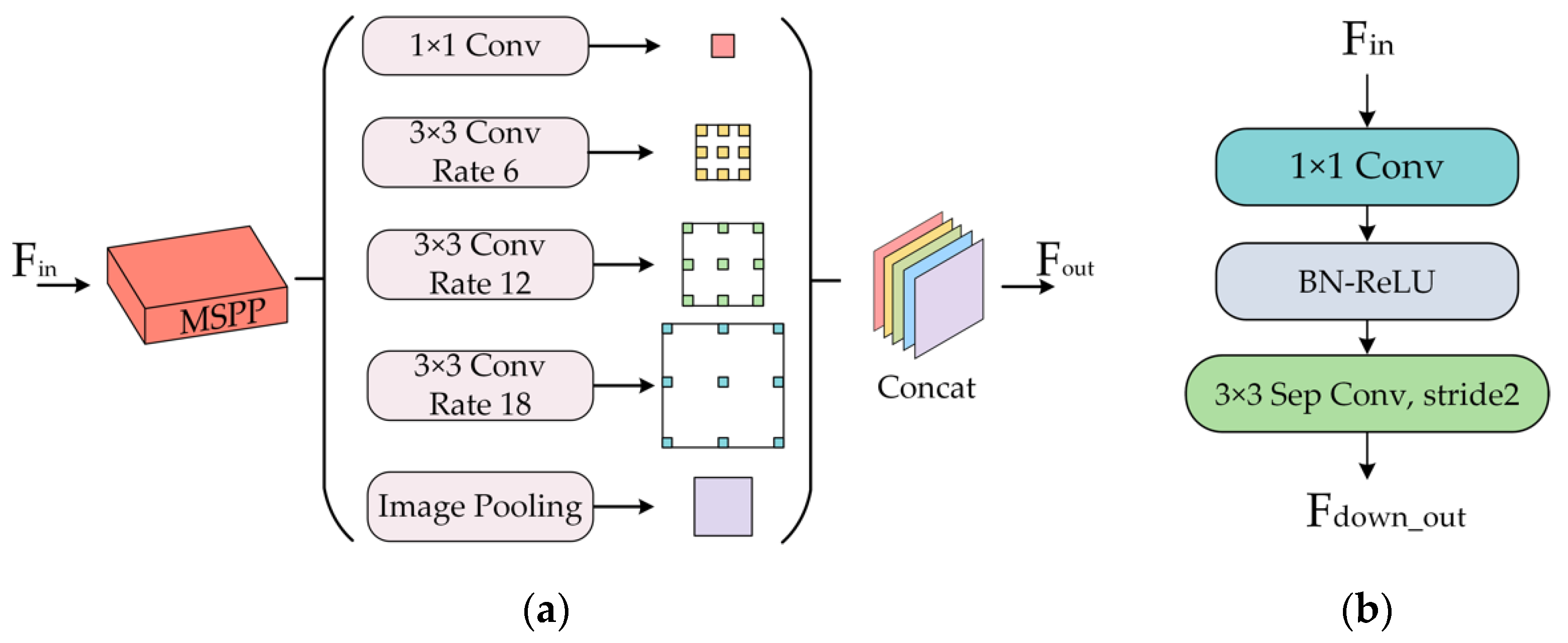
To address the challenges, we created a Landsat 8 water body dataset: Landsat River dataset (LR dataset), and proposed a new semantic segmentation network, namely Dense U-Net+ network (DUPnet), for water bodies in remote sensing images. This model takes global contextual information, multi-scale information, and feature information into account in order to (1) extract multi-scale information for skip connections and alleviate the gradient vanishing problem, we build the multi-scale spatial pyramid pooling module (MSPP); (2) to extract features at different levels, e.g., low-level features and highly abstract features, we introduce Dense Block [27] to enhance feature propagation and encourage feature reuse; (3) to obtain a better segmentation performance, we use multiple levels of features for pixel-level image semantic segmentation.
When designing a complex deep learning model, the choice of loss functions is also important as they stimulate the learning process. Since 2012, researchers have experimented with loss functions in various fields to improve the results of their datasets. Jadon [28] summarized 15 loss functions based on image segmentation that have been shown to provide excellent results in different fields. These functions can be classified into four categories: distribution-based [29,30], region-based [31,32], boundary-based [33,34], and compounded [35,36]. We finally used a regression loss function with a mixture of distribution-based cross-entropy loss and region-based Tversky loss for training. Cross-entropy [37] is defined as a measure of the difference between two probability distributions for a random variable or event set and has been frequently used for pixel-level classification segmentation. However, cross-entropy has an obvious drawback when the image segmentation task requires only two cases to be segmented: foreground and background. When there are fewer foreground pixels, the background component of the loss function dominates, resulting in low segmentation accuracy. Furthermore, the Tversky index [38] can increase the weighting of false positives and false negatives, which effectively address the problem of data imbalance.
The main contributions of this study include the following:
(a)
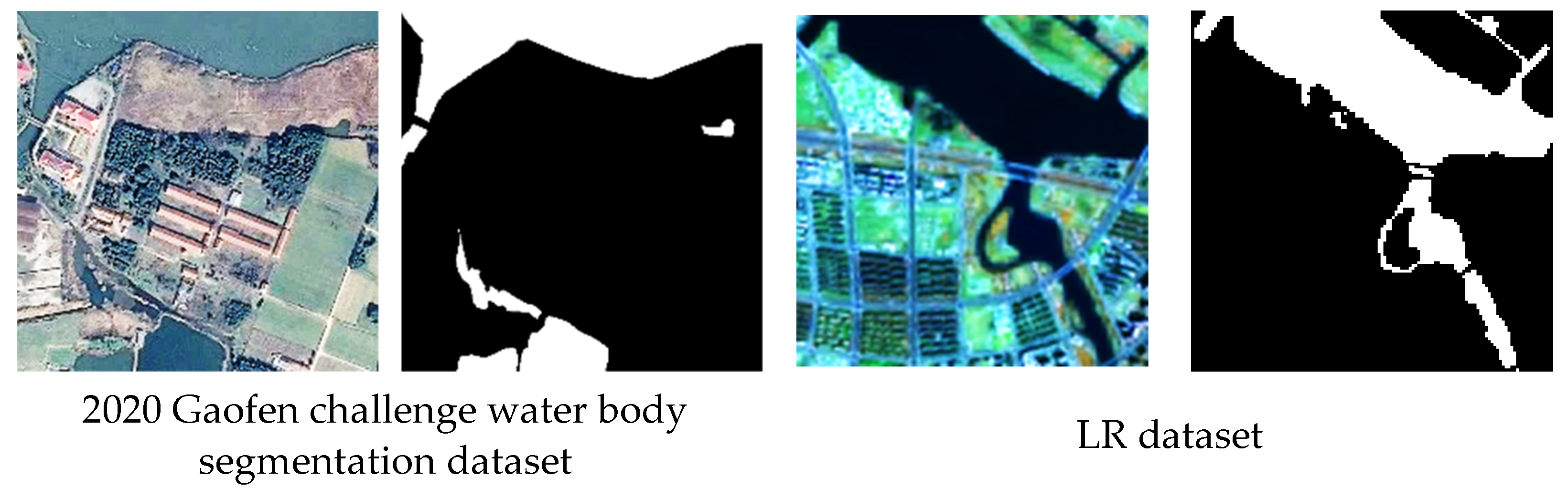
A network framework (DUPnet) is proposed by combining the MSPP and dense block to segment water bodies from remote sensing images. The DUPnet uses multi-scale spatial features and multiple levels of spectral features. The experimental results on the 2020 Gaofen challenge water body segmentation dataset and the LR dataset show that the DUPnet model outperforms the majority of state-of-the-art segmentation methods, and the FWIoU for these two datasets are 93.52% and 91.77%, respectively.
(b)
A water body classification dataset is proposed based on Landsat 8 OLI images, namely the LR dataset, which contains 7154 images with 128 × 128 pixels and covers an area of ~ 34,225 km2 of the Yellow River in the Henan region, China. The LR dataset can provide the research community with high-quality datasets when conducting the water body classification for Landsat imagery.
(c)
A regression loss function (Log-Cosh Tversky Loss, all for short LCTLoss) was developed based on the Tversky index to address the imbalance of positive and negative samples. By modifying hyperparameters, our method is able to distinguish the water bodies with substantial edge changes. The experimental results on the LR dataset show that our proposed loss function outperforms Cross-Entropy (CE) Loss, Binary Cross-Entropy (BCE) Loss, Focal Loss, Dice Loss, and Tversky Loss, demonstrating the effectiveness of the proposed loss function.

2. Methods and Materials

2.1. Methods

2.1.1. Main Network Structure

As shown in Figure 1, we propose a DUP network based on the U-Net encoder–decoder network in conjunction with the dense block (DB) and the MSPP of DeeplabV3+. Specifically, the DUP network contains three parts: encoder, decoder, and skip connection, respectively. The encoder consists of convolutional layers (Conv), Batch Normalization (BN) [39], Rectified Linear Units (ReLU) [40], four dense blocks, and four down-sampling (Down) layers. The decoder uses five dense blocks and four up-sampling (Up) layers to recover the features. Skip connection uses the MSPP, and the segmented image is finally output by a classification layer.
Main features of the DUP network:
(1)
The encoder and decoder primarily use dense blocks, which are used to improve the network’s ability to extract image semantic features and obtain highly abstracted feature maps.
(2)
Skip connections employ the MSPP based on Atrous Convolution to improve the feature utilization and compensate for the feature loss.
(3)
Down-sampling (Down) module that uses Atrous Separable Convolution (Sep Conv) [15] instead of the maximum pooling layer to increase the perceptual field of the feature map and improve the robustness of the network model.
Specifically, the DUP network uses the DB of DenseNet to establish connections between different layers, alleviate the problem of gradient disappearance, and enhance feature propagation to obtain clearer segmentation. As shown in Figure 2, one of the dense blocks assumes that the network has l layers, and layer l will accept the output features of all the predecessor network graphs as the input of layer l. The output of layer l is represented by a x l and x l is defined as:
x l = H l ( { x 0 , x 1 , , x l 1 } )
where H l ( ) represents the nonlinear transformation function, which is a combined operation including a series of BN, ReLU, and Conv operations.
Each DB contains four 1 × 1 convolutions, four 3 × 3 convolutions, and four feature fusions, as shown in Figure 2. The number of input feature maps can be reduced by introducing a 1 × 1 convolution before each 3 × 3 convolution. The BN and ReLU layers are added after each convolution layer of the DB [39].
In the BN layer, the mean and standard deviation computed for each batch are approximate estimates of the global mean and standard deviation, which introduces randomness into our search for the optimal solution and thus acts as a regularization.
An activation function is a function introduced to an artificial neural network to provide nonlinearity and enhance the expressive capability of the network. In this study, ReLU is chosen as the activation function. Firstly, using the ReLU activation function can save a lot of computation when back propagating to find the error gradient. Using functions such as the Sigmoid activation function involves division, which is computationally intensive and prone to gradient disappearance during back propagation. Secondly, ReLU can make the network sparse, reducing the interdependence of parameters and alleviating overfitting.
As shown in Figure 3a, skip connections leverage the MSPP to combine shallow data from the encoding stage with deep information from the decoding step. Skip connection facilitates feature fusion in the U-Net network by clipping shallow features and splicing them with deep features. This strategy is not useful, as it causes the skip connection’s output to be a specific region in the input’s center, which will affect the accuracy of feature extraction from the image’s edges. In the DeeplabV3+ network, the ASPP scheme uses multiple parallel Atrous Convolutional Layers with various dilation rates to increase the perceptual field. The MSPP constructs the results by extracting the multi-scale features from the encoder layer output and fusing them with the decoder layer output, resulting in more dense multi-scale feature data. The MSPP is used as the skip connection in the DUPnet network.
The maximum pooling reduces the spatial resolution of the produced feature maps, which causes feature information loss. As a result, as shown in Figure 3b, the down-sampling module replaces the original maximum pooling layer with a 3 × 3 null separable convolutions (Sep Conv) with a stride of 2. This convolution is a depth-separable convolution with stride, which decomposes the standard convolution into the Depthwise Convolution [41] and the Pointwise Convolution. As shown in Figure 4, the Depthwise Convolution has a broader sensory field, which can effectively improve the shortcomings of maximum pooling. Deep convolution uses spatial convolution for each channel independently, with pointwise convolution used to integrate the results. Convolution with depth separation can considerably reduce the number of parameters and processing effort. Null convolution may extract more features response by increasing the null rate and enabling larger overlapping sampled regions on the input feature map at each sampling, but conventional convolution can only extract small chunks of features when the number of parameters is known. Null-separable convolution not only reduces feature loss but allows for feature extraction on feature maps of any resolution.
The up-sampling operation uses transposed convolution to increase the spatial dimensionality of the feature map. For pixel-level segmentation, the image size needs to be restored to its original size. The feature map output from the network’s middle layer is deconvolved to pixel space by deconvolution.
The parameters of each layer in the DUP network are set as shown in Table 1.

2.1.2. Main Network Tversky Coefficients-Based Regression Loss Function

In the field of computer vision, the Dice coefficient is a frequently used statistic for calculating picture similarity. It has also been refined into a loss function, Dice Loss [31]. The Tversky Index (TI) [38] is an extension of the Dice and Jaccard coefficients, and the Tversky Index is defined as follows:
T I = y t y p y t y p + β ( 1 y t ) y p + ( 1 β ) y t ( 1 y p )
The Tversky coefficient is the Dice coefficient when β = 0.5, while the Tversky Index is the Jaccard coefficient when β = 1. The trade-off between false positives and false negatives can be controlled by adjusting the hyperparameter β. In Equation (3), β = 0.7. Tversky Loss (TL) is defined as follows:
T L = 1 1 + y t y p 1 + y t y p + β ( 1 y t ) y p + ( 1 β ) y t ( 1 y p )
As Tversky Loss supports the mathematical formulation of the segmentation objective, Tversky Loss has also been adapted for use as a loss function. However, as it is non-convex, Tversky Loss may not produce optimal outcomes. As for regression-based problems, Log-Cosh has been commonly utilized to smooth the curve [28]. In terms of nonlinearity, deep learning algorithms have used hyperbolic functions, such as tan layers, which are simple to manage and identify. The functional expression of cosh(x) is defined as follows:
cosh ( x ) = e x + e ( x ) 2
However, the range of cosh(x) can rise to infinity. Therefore, to facilitate the calculation in the range of values, the log function is used, and log(*) is a logarithmic function with the natural number e as the base. The expression of the Log-Cosh function is defined as follows:
L ( x ) = log ( cosh ( x ) )
The derivative of L(x) with respect to x is (6):
L ( x ) = sinh ( x ) cosh ( x ) = tanh ( x )
As the range of tan(x) is (−1, 1), L(x) is continuous and finite. Log-Cosh will remain continuous and finite after first-order differentiation, according to the foregoing proof. In this study, we present the Log-Cosh Tversky Loss function (LCTLoss), which is simple to construct while retaining the properties of the Tversky coefficient and cross-entropy. LCTLoss is defined as follows:
L C E = [ ( y t ) log ( y p ) + ( 1     y t ) log ( 1 y p ) ]
L L C T = L C E + log ( cosh ( T I ) ) 2
where yt is the true value of the prediction model, and yp is the predicted value of the prediction model.

2.1.3. Implementation Details and Evaluation Indexes

All experiments were run on an NVIDIA GeForce RTX 3070 graphics card with Python 3.8 and PyTorch 1.9.0 on Windows 10. The network model was optimized with the RMSprop [42] optimizer, which iterated until the best model was found. 5 × 10⁻⁴ and 0.90 were used as the weight decay and momentum parameters, respectively [23]. The model was trained for 150 epochs using a batch size of 8 epochs, an initial learning rate of 0.001, and the learning rate was dynamically adjusted using the poly method [43].
The evaluation metrics used in this paper include Recall, Precision, Accuracy, Mean Intersection over Union (MIoU), Frequency Weighted Intersection over Union (FWIoU), and F1 and are shown as follows:
R e c a l l = T P T P + F N ,
P r e c i s i o n = T P T P + F P ,
A c c u r a c y = T P + T N T P + T N + F N + F P ,
M I o U = 1 k + 1 i = 0 k T P T P + F P + F N ,
F W I o U = T P + F N T P + T N + F N + F P × T P T P + F P + F N ,
F 1 = 2 × R e c a l l × P r e c i s i o n R e c a l l + P r e c i s i o n
The confusion matrix between the water body masks and ground truths is calculated, consisting of true positives (TP), true negatives (TN), false positives (FP), and false negatives (FN). The positive and negative represent water and background, respectively.

2.2. Materials

To validate our approach, we conducted experiments on the 2020 Gaofen challenge water body segmentation dataset [44] and the Landsat River dataset created in this study. Figure 5 shows a sample image and mask from these datasets.

2.2.1. Gaofen Dataset

We chose the 2020 Gaofen Challenge Water Segmentation Dataset, which is the only high-resolution optical dataset for water body classification. The dataset contains 1000 RGB images from the GF-2 satellite with a pixel resolution of 1–4 m and an image size of 492 × 492. We expanded to 8000 images by rotating, blurring, brightening, darkening, and adding noise. This dataset was partitioned into training, validation, and test sets with a scale of 6:2:2.

2.2.2. Landsat River Dataset

Based on the remote sensing images of the Yellow River in the Henan region, we created a new dataset called the Landsat River dataset (LR dataset) to further evaluate the performance of the proposed network. Images from Landsat 8 satellite were downloaded freely from the USGS website (https://earthexplorer.usgs.gov/, accessed on 24 August 2022). The Landsat 8 remote sensing satellite is made up of two sensors, Operational Land Imager (OLI) and Thermal Infrared Sensor (TIRS), which can provide some daily images at 16-day intervals. Each scan generates an image with an area of ~34,225 km2. The optical remote sensing data in this study are collected from the Landsat 8 OLI, and the specific information used in the experiment is shown in Table 2.
The raw remote sensing images are processed using the ENVI 5.6.1 platforms (Exelis Visual Information Solutions, Boulder, CO, USA) [45], which includes pre-processing, water-body masking, and data set delineation.
The main steps of pre-processing are as follows:
(1)
The multispectral band data with a resolution of 30 m and the panchromatic band data (Band 8) with a resolution of 15 m are sharpened using the Brovey Transform [46] to obtain the high-resolution remote sensing image (15 m) and preserve the multispectral information.
(2)
The radiometric calibration operation is used to reduce errors generated by the sensor itself, the atmospheric correction operation is used to recover the spectral information of features, and the orthorectification operation is used to avoid geometric distortions in the image.
(3)
The bands NIR (Band 5), SWIR1 (Band 6), and Red (Band 4) as selected as the red, green, and blue channels, respectively, to obtain the false color composite images. The combined false color composite images are easier to identify water bodies, rivers, lakes, and other large and small pools. These pre-processing steps are illustrated in Figure 6.
Support Vector Machine (SVM) [47] is a nonparametric statistical method used to solve supervised classification and regression issues. The underlying assumption is that separating two classes in the feature space is analogous to establishing an appropriate hyperplane, at least for linearly separable variables [48]. Determining a separation hyperplane geometrically is equal to identifying specific observations, known as support vectors, that best describe the problem’s classes. The marginal parameters define the degree of separation between the data as well as the number of support vectors required by the model.
With the advent of support vector machines [48,49], the accuracy and efficiency of remote sensing image classifying are greatly improved, resulting in a competitive option for remote sensing applications on sample masking [50]. We use the SVM classifier based on the ENVI 5.6.1 platforms to generate a water body mask and set the kernel type of the SVM classifier to Polynomial; other parameters refer to the official ENVI document [51].
The main steps to create the dataset include:
(1)
SVM classifier: The images described in Table 2 are selected as training and validation data. Due to the large size of these three images, we use the ENVI software platform to divide each image into four parts, where one-quarter of each image is used for SVM classifier training, and the remaining three-quarters are for validation. Taking the image dated 2021/03/22 as an example, the following steps are performed:
(a)
The ROI (Region of Interest) tool is used to construct the region of the water body (training sample).
(b)
The SVM classifier is then applied to extract water bodies.
(c)
The Interactive Class Tool is utilized to manually modify the misclassified or omitted image attributes, and water body spectral curves were utilized to assist in this work to obtain the classification results of the water bodies.
(d)
The water body classification results are transformed into ROI to extract the water bodies, and then repeat steps (b) and (c) to obtain the water body extraction results of the complete remote sensing images.
(2)
Image selection: The images are cropped to the water-body masks of remote sensing images and the remote sensing images corresponding to the water-body masks into 128 × 128 size images. In addition, the water body masks are manually corrected again in the cropped images to form the LR dataset, which contains 7154 images. This dataset was partitioned into training, validation, and test sets with a scale of 6:2:2.
(3)
Image augmentation: Data augmentation [52] is undertaken before model training and improves sample diversity and the training model’s generalization performance. In the remote sensing image water-body dataset, image enhancement is conducted on all images in the training set and validation set by conducting horizontal flip [53], random Gaussian blurring [54], and normalization [55].

3. Results and Discussion

3.1. Ablation Study

3.1.1. Quantitative Comparison of Ablation Study

Using U-Net as a baseline, an ablation experiment analysis is performed in this work to test the efficiency of MSPP and Dense Block (DB). Where MSPP is introduced into U-Net as a skip connection and DB replaces the original convolutional layer of the U-Net structure. Firstly, to investigate the effect of different dilation rates on MSPP, three distinct dilation rates were chosen: {1, 6, 9, 12}, {1, 6, 12, 18}, and {1, 12, 24, 36}. As shown in Table 3, with the increase in dilation rate, F1 and MIoU increase first and then decrease. A dilution rate of {1,6,12,18} resulted in the highest F1, MIou, and FWIoU (Table 3). When the dilation rate is low, the model is less accurate in predicting difficult-to-classify pixels but more accurate in predicting easy-to-classify pixels. The prediction of hard-to-classify pixels may improve, but the prediction of easy-to-classify pixels may degrade. Therefore, we chose a dilation rate of {1, 6, 12, 18} in this study, which can make the MSPP more effective.
To ensure that the MSPP and DB approaches contribute to the results of water segmentation. As shown in Table 4, adding the MSPP module to U-Net can enhance F1, MIoU, and FWIoU by 1.2%, 2.69%, and 2.79%, respectively, indicating that the MSPP is efficient in water segmentation. The addition of the DB module to U-Net only increases the MIoU by 0.17%, but the addition of the DB module makes the network extract more water body pixels, as shown in Figure 7 and Figure 8. The DUPnet uses MSPP for skip connections and DB modules; its F1, MIoU, and FWIoU increase by 1.84%, 4.96%, and 4.47%, respectively, compared to U-Net.

3.1.2. Qualitative Comparison of Ablation Study

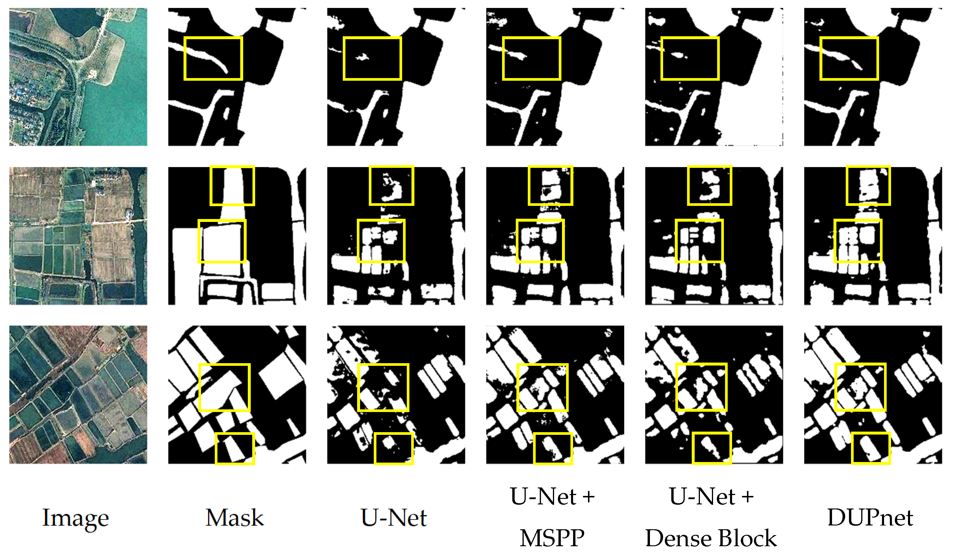
This study analyzes the segmentation features created independently before and after using the MSPP and DB to visually confirm the effectiveness of the proposed module. The study uses yellow boxes to highlight the locations where there are discrepancies in identification. Figure 7 and Figure 8 depict the effect of the original U-Net, the U-Net with MSPP as skip connections, and the U-Net with DB as a convolutional layer for segmenting water bodies.
As shown in Figure 7, the U-Net with the MSPP and DB module recognizes more water from the input image, extracts more features, and improves recognition of difficult-to-extract regions such as shadows than the original U-Net.
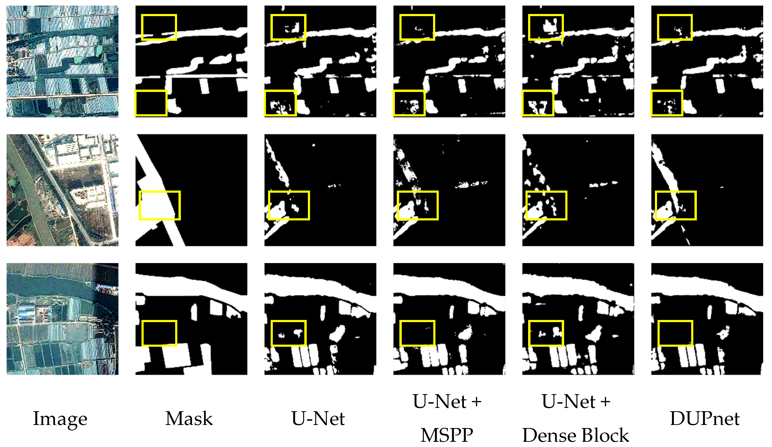
As shown in Figure 8, comparison images monitor small water bodies, the original U-Net can only track a tiny percentage of narrow streams on the input image. The addition of MSPP and DB modules can improve the model’s ability to locate water bodies, extract small water bodies, and reduce water body misclassification and omission.

3.2. Quantitative and Qualitative Comparison with State-of-the-Art Methods

3.2.1. Quantitative Comparison with State-of-the-Art Methods

To comprehensively evaluate the segmentation performance of the improved DUPnet model, eight segmentation networks, FCN, SegNet, U-Net, ENVINet5 [56], PSPNet, DeepLabV3+, HRNet V2, and Maximum Likelihood Classification (MLC) [57], were chosen for comparison in this study, and the performance of the trained models was tested using the test set. The FCN, SegNet, U-Net, PSPNet, DeepLabV3+, HRNet V2, and DUPnet networks were trained using the network parameter settings in Section 2.1.3, with the same backbone network Resnet50 used for FCN, PSPNet, and DeepLabV3+. In addition, the best hyper-parameters of the segmentation algorithms were used in the comparison approach.
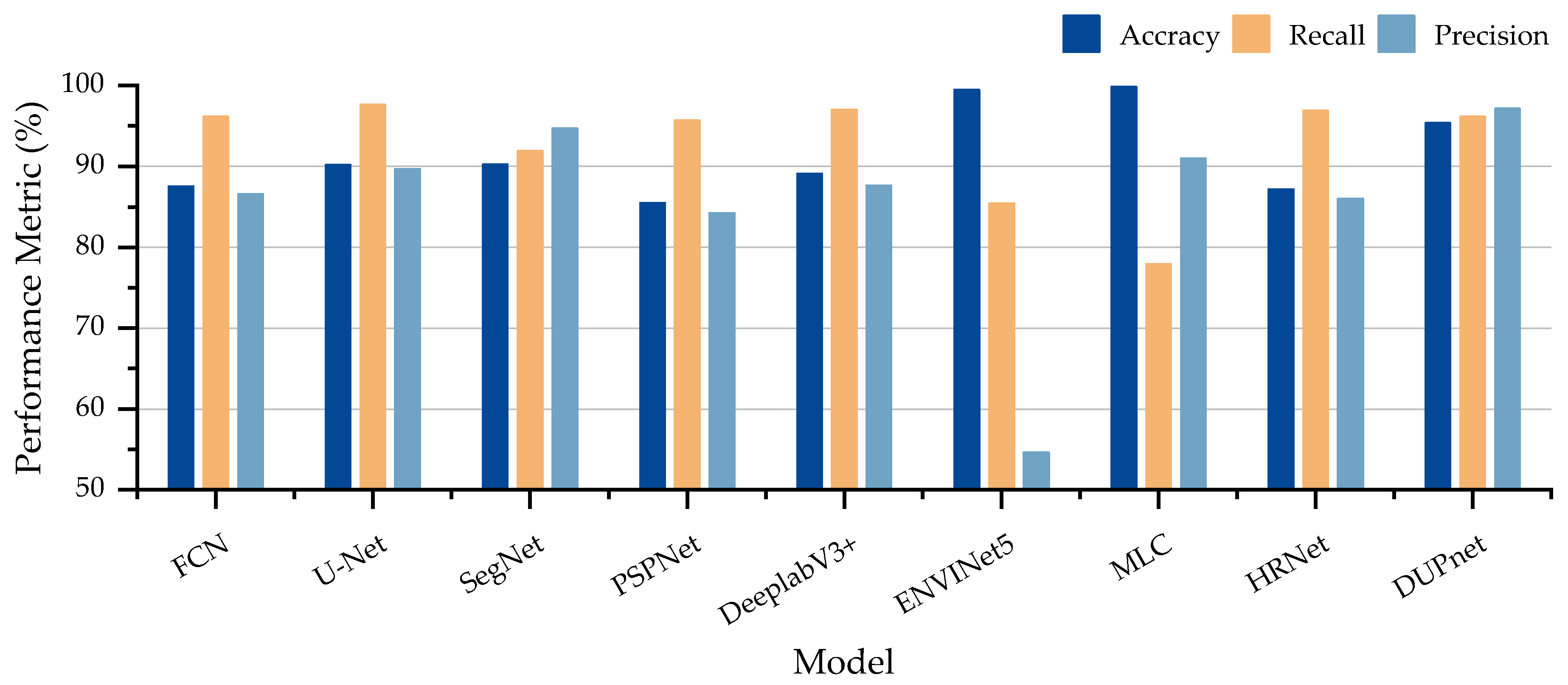
As shown in Table 5 and Figure 9, the results of the competence evaluation comparison between DUPnet and other network segmentation results on the LR dataset. The probabilistic discriminatory rules-based MLC has the highest Accuracy of 99.82%; the U-Net performs the best in Recall with 97.62%; the proposed DUPnet has the highest Precision of 97.15%.
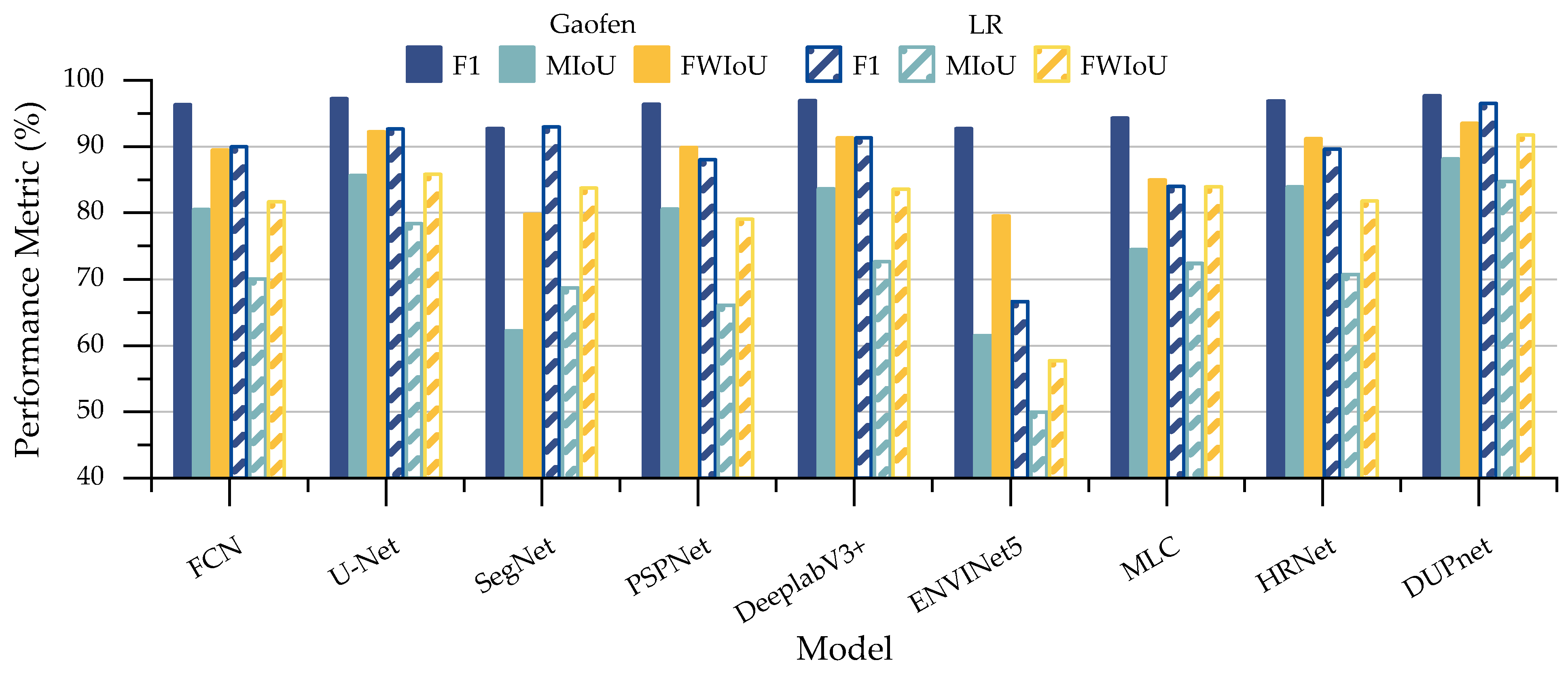
Table 6 and Figure 10 provide the comparison of our method with state-of-the-art methods on the 2020 Gaofen challenge water body segmentation dataset and the LR dataset in F1, MIoU, and FWIoU. In the case of both datasets, DUPnet achieves the most superior performance for each of the three metrics because DUPnet uses both dense blocks, contextual aggregation, and multi-scale skip connection, which gives it an advantage over the other methods.
As shown in Table 7, to evaluate the complexity of the compared models, the size of the memory occupied by the model files and the average time used to predict one image (model input is 1 × 3 × 128 × 128) in the test dataset after training by FCN, U-Net, SegNet, PSPNet, DeepLabV3+, HRNet V2, and DUPnet. The U-Net used the maximum pooling layer in 4 down-sampling operations, and the feature layer 4 compressions are performed, U-Net’s model file has the smallest file size (153 M) and average prediction time (0.2500 s) when compared to the remaining five methods. As PSPNet uses ASPP to enlarge the receptive fields, it has the longest model file size (534 M) and average prediction time (0.5556 s) when using the same backbone network Resnet50 as FCN and DeeplabV3+. The DUPnet proposed in this work does not use a backbone network, but dense blocks in the feature propagation process replace maximum pooling with Atrous Separable Convolution in the down-sampling process, which has a higher feature utilization. The DUPnet has a relatively small model size (296 M) and average prediction time (0.4444 s).
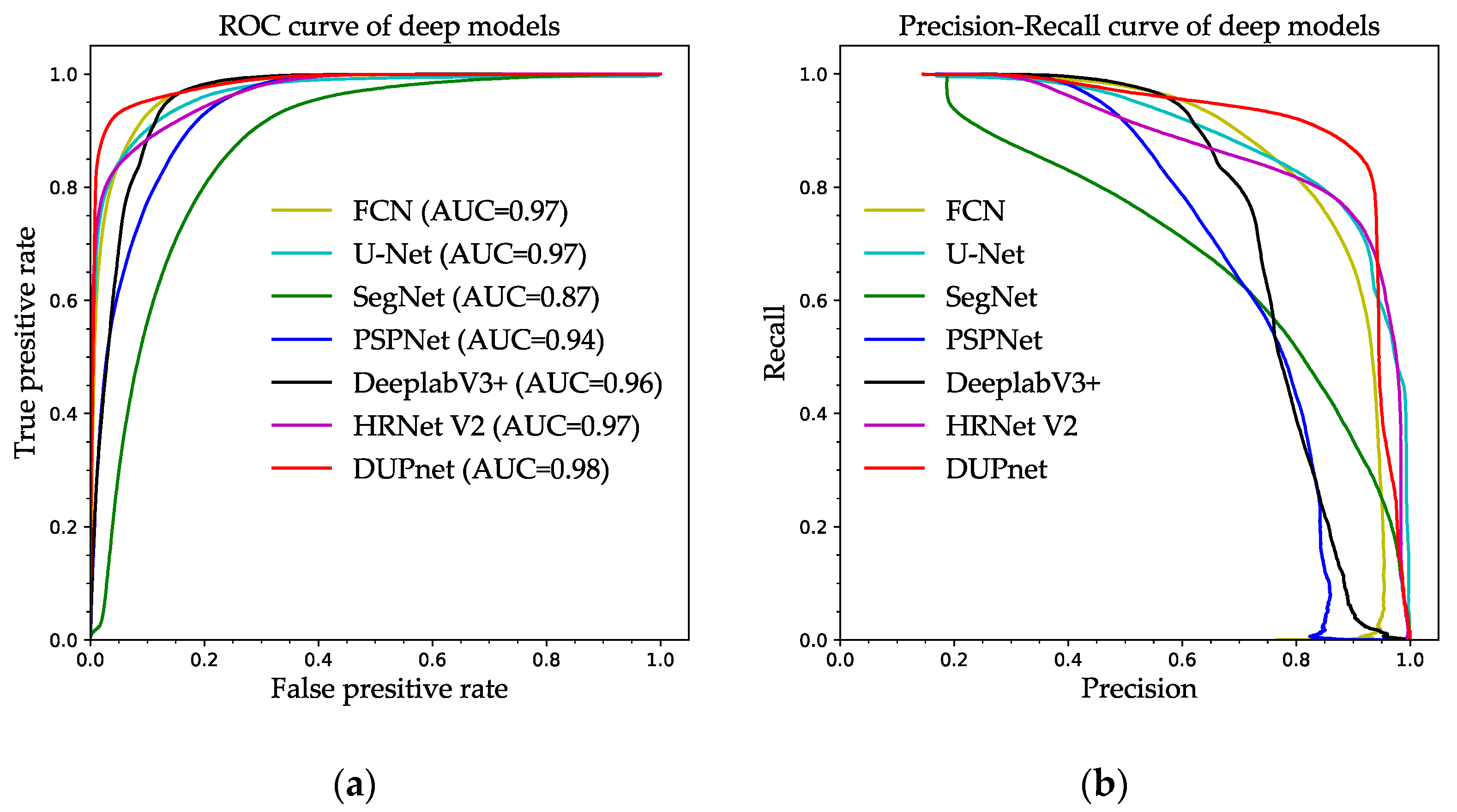
To evaluate the segmentation ability of the compared models, the evaluation of the water segmentation ability of the models of FCN, SegNet, U-Net, PSPNet, DeepLabV3+, and DUPnet in the LR dataset after the completion of training using ROC (Receiver Operating Characteristic) curves and P–R curves are shown in Figure 11a,b. AUC (Area under Curve), the area under the Roc curve, is between 0.1 and 1. AUC is a value that can visually evaluate the goodness of the classifier. A larger value of AUC represents a better result. In the P–R curve diagram, if the curve bend towards the upper right corner, i.e., (1, 1), the segmentation performance of the corresponding model is better. SegNet has an AUC of 0.87 and has the smallest area under the ROC curve and the P–R curve. Therefore, it had the worst performance for segmentation. The proposed DUPnet has an AUC of 0.98 and contains the largest area under the ROC curve. The P–R curve of DUPnet is closer to the upper right corner compared to the other methods. Therefore, the ROC and P–R curve plots indicate that the proposed DUPnet has better model segmentation ability when compared to other methods.

3.2.2. Qualitative Comparison with State-of-the-Art Methods

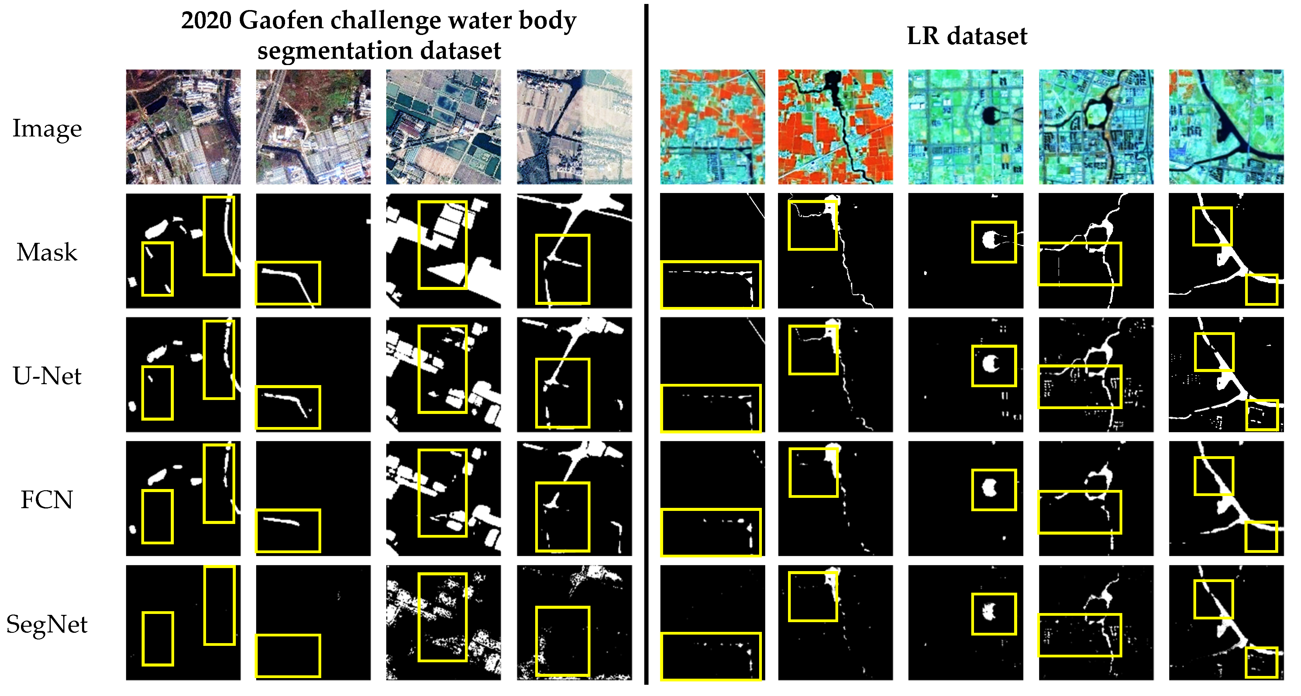
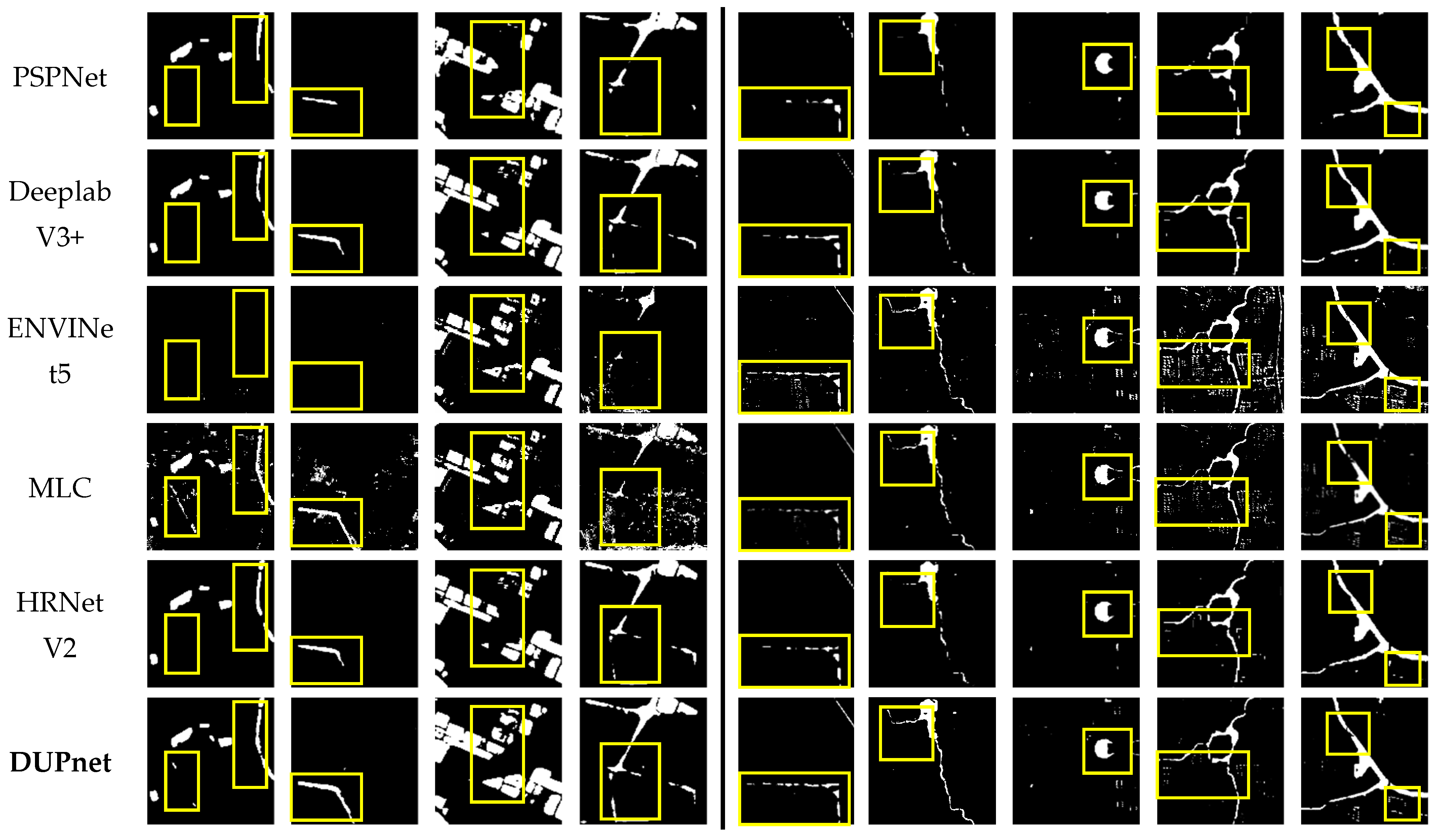
A qualitative comparison of the performance of the proposed method and comparable methods on the LR dataset and the 2020 Gaofen challenge water body segmentation dataset was also conducted. 
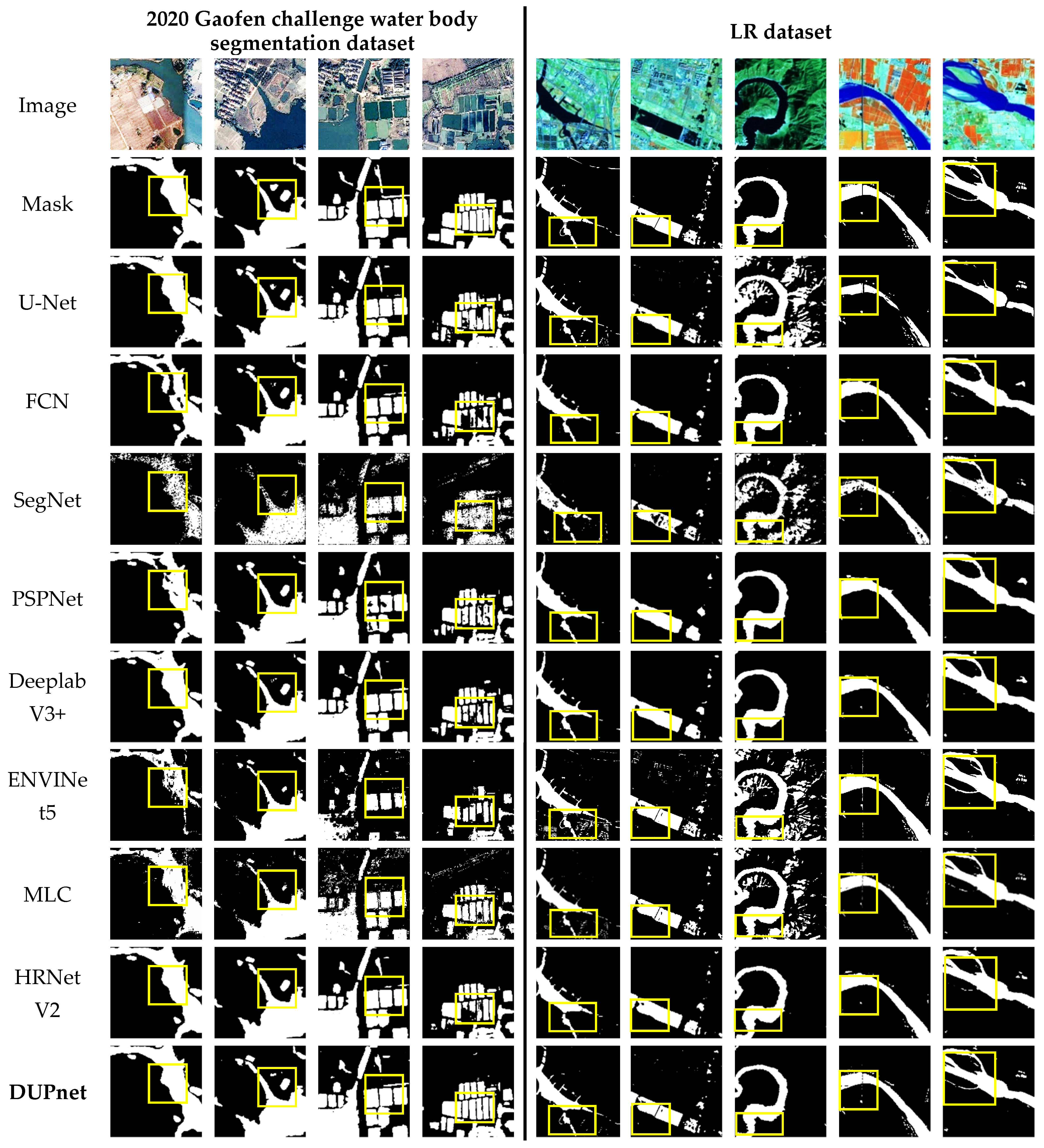
Figure 12 depicts the qualitative evaluation in comparison to several methodologies.
Figure 12 presents examples of water bodies extraction results from the Gaofen dataset in the first through fourth columns. From the results, our proposed deep segmentation network DUPnet can integrate the properties of three networks, including codec structure, dense connection, and Atrous Convolution, to increase the extraction accuracy of water bodies of various types (rivers, water fields, and water channels).
The images in columns 5 and 6 of Figure 12 show urban waters of various sizes and shapes of our created LR dataset. FCN, PSPNet, and DeeplabV3+ have unclear boundary segmentation of urban waters, and small water bodies in the city are not detected, but the discrimination ability of error-prone sub-pixels such as urban building shadows is good. SegNet has poor discrimination ability for the central region of water bodies. U-Net, ENVINet5, and MLC are effective in extracting urban water bodies of various sizes, but hard-to-identify regions such as urban building shadows are misclassified as water bodies.
As shown in column 7 of Figure 12, the image background is a mountain of the LR dataset, FCN, PSPNet, and DeeplabV3+ have high accuracy and less error for pixel segmentation of water bodies in the mountains. U-Net, SegNet, ENVINet5, and MLC are easy to confuse hill shadows and water bodies, and the segmentation accuracy is not very high. The proposed DUPnet retains a lot of spatial details for the segmentation of water bodies in the mountains, the edges are clearer and more accurate, and these easily mis-segmented pixels of the hill shadows can be well distinguished.
The images in columns 8 and 9 of Figure 12 show rivers of varying widths of the LR dataset, and the river water bodies segmented by U-Net are discontinuous, whereas the other approaches find continuous water bodies. SegNet segments river water bodies with gaps, while the ENVINet5 misclassifies roads with a similar color to water bodies as water bodies. FCN, PSPNet, DeeplabV3+, and MLC have a poor resolution for river tributaries. The proposed DUPnet is continuous and can discriminate the hard-to-identify river tributaries. This model produces water-body segmentation images on the LR dataset with more clear and more accurate segmentation edges and retains more water-body details.
In addition, as shown in Figure 13, FCN, SegNet, PSPNet, and DeeplabV3+ distinguish building shadows with the best result, but the recognition of small waters is less evident; U-Net, ENVINet5, and MLC identify more building shadows as water bodies; our proposed method has a complete and clear boundary, and identifies more water pixels, which has the best segmentation performance on narrow streams and point water.

3.3. Comparative Analysis of Different Loss Functions

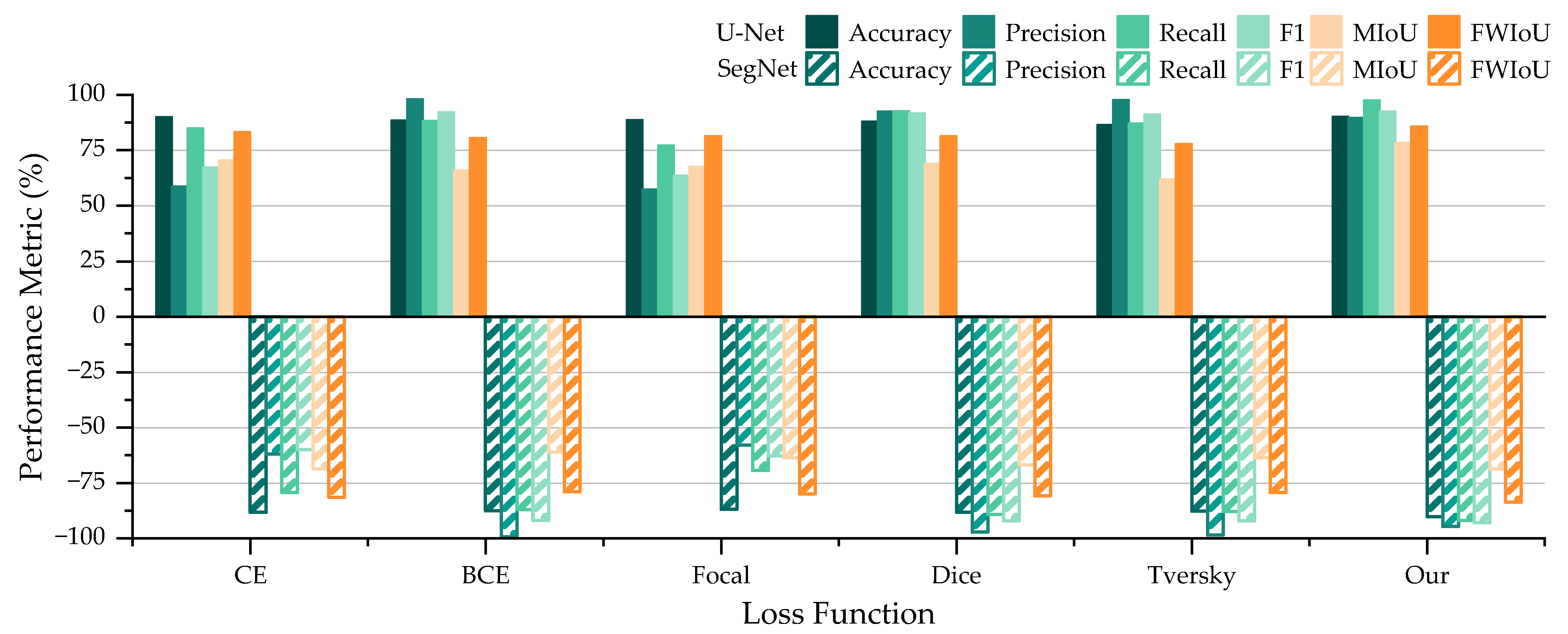
Additionally, on the LR dataset, we conduct a comparative experiment for the Cross-Entropy (CE) Loss, Binary Cross-Entropy (BCE) Loss, Focal Loss, Dice Loss, Tversky Loss, and our proposed LCTLoss to evaluate the effects of different loss functions on model performance.
We evaluated the performance of U-Net and SegNet under six different loss functions (Table 8 and Figure 14). U-Net achieved the optimal results using our proposed LCTLoss where Accuracy, Recall, F1, MIoU, and FWIoU proposed in this work are 90.23%, 97.62%, 92.67%, 78.37%, and 85.85%, respectively. SegNet achieved the optimal results using our proposed LCTLoss in this paper, where the Accuracy, Recall, F1, and FWIoU are 90.30%, 91.96%, 93.00%, and 83.74%, respectively.
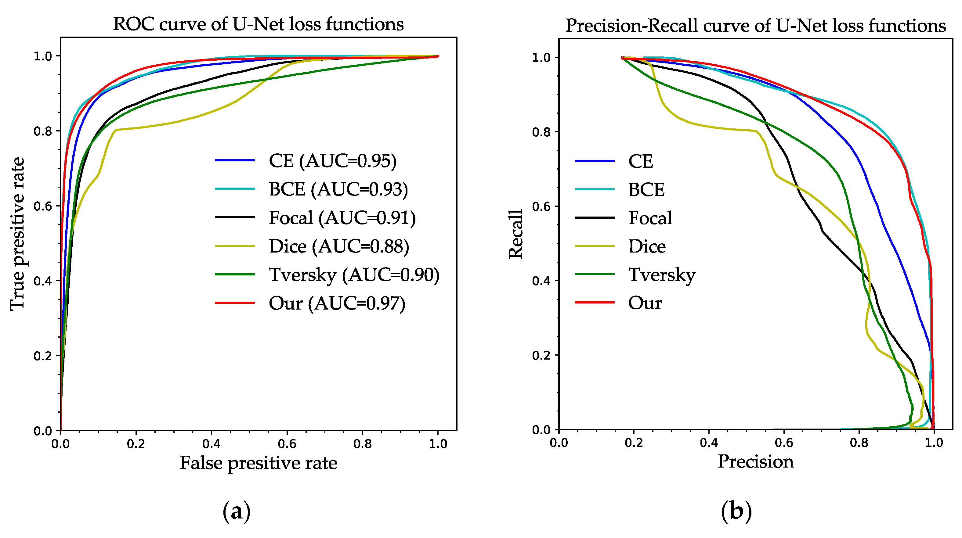
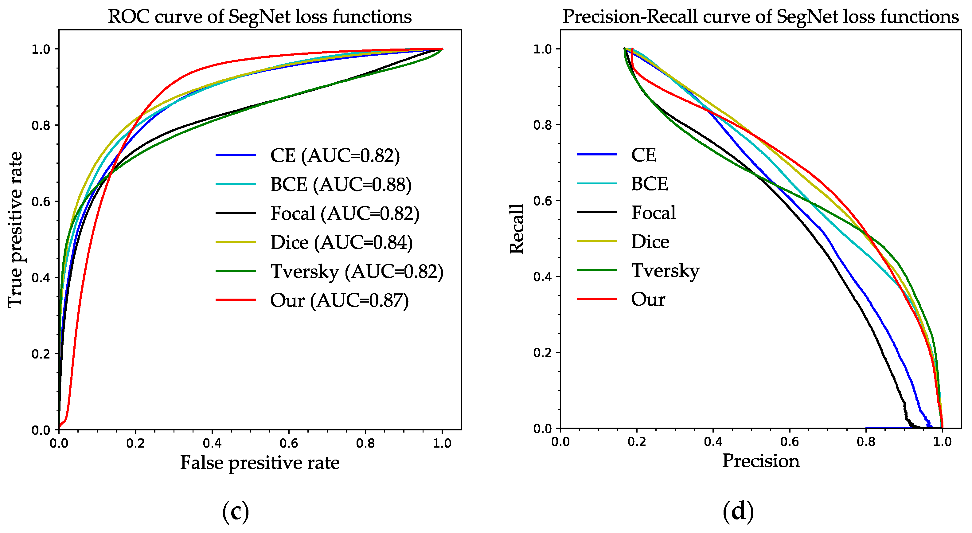
We evaluated the impact of six loss functions on the segmentation ability of U-Net and SegNet by using ROC curves and P–R curves (Figure 15). It can be seen from Figure 15a that the U-Net model performed the best using our loss function with an AUC of 0.97 on the ROC curve and the worst using Dice loss with an AUC of 0.88. According to Figure 15b, U-Net has the closest curve to our loss function and the BCE loss on the P–R curve, but the curve representing the red curve of our loss function contains a large area under the curve, so our loss function is better, while the curve of dice loss contains the smallest area under the curve, so the segmentation ability is inadequate.
As shown in Figure 15c,d, the SegNet evaluates the effect of six loss functions on the segmentation ability of the model using the ROC curve and P–R curve. According to Figure 15c, the BCE loss performs best on the ROC curve for the SegNet model, with an AUC of 0.88, while the Tversky Loss and Focal Loss both perform poorly, and both have equal AUC of 0.82. From Figure 15d, on the P–R curve, the SegNet has the best segmentation ability, with the curve of our loss function closest to the top-right vertex and the curve of Focal Loss closest to the coordinate origin, indicating that the segmentation effect is undesirable.
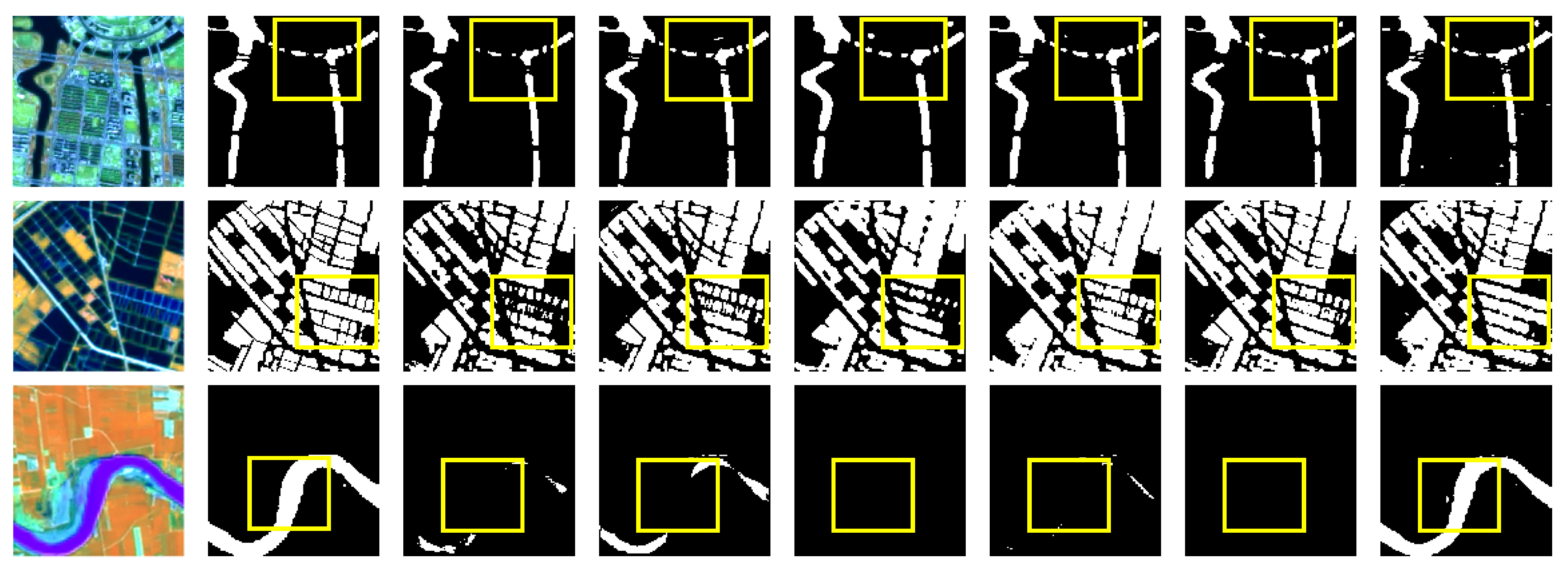
Some representative images for analyzing and observing the performance of the six loss functions are shown in Figure 16 and Figure 17, which represent a qualitative comparison of U-Net and SegNet for water body segmentation using these six loss functions, respectively. It can be seen from lines 1 and 2 of Figure 16 that U-Net identifies more pixels of the water bodies using our loss function. Lines 3 and 4 of Figure 16 show that U-Net only uses our loss function to segment the complete water bodies with clear boundaries. Line 5 of Figure 16 shows that U-Net makes Dice loss, and our loss function to identify more water bodies, but the water-body boundaries are not clear. As our proposed loss function set a fixed hyperparameter β, which does not reach the optimal positive and negative sample balance, it may have an effect on some water body pixels that are hard to distinguish. In this regard, we will continue to investigate the adaptive hyperparameter of the loss function in the future.
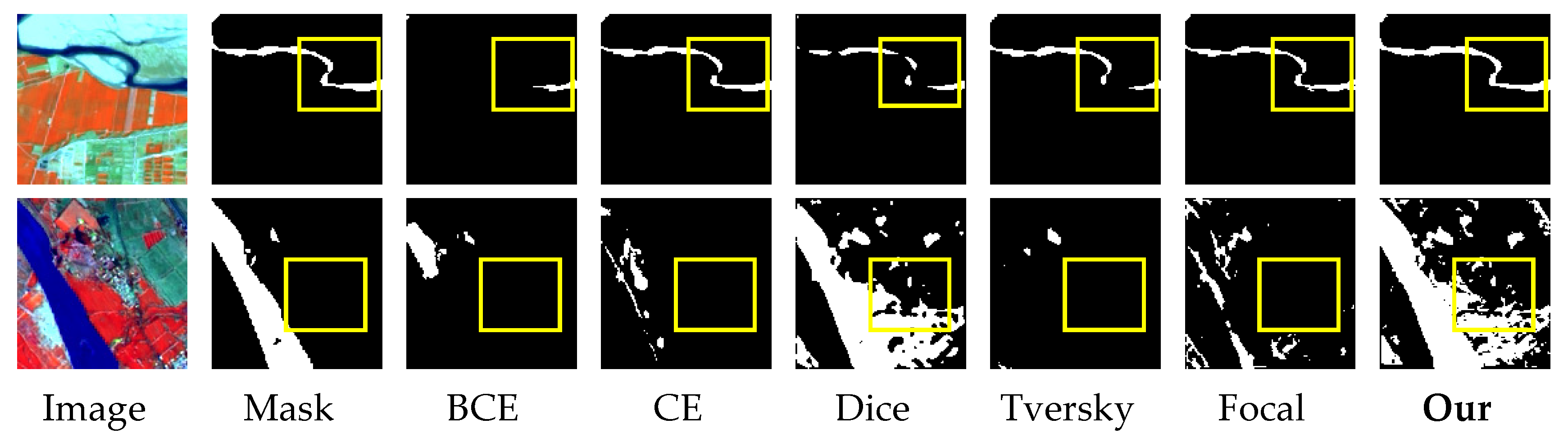
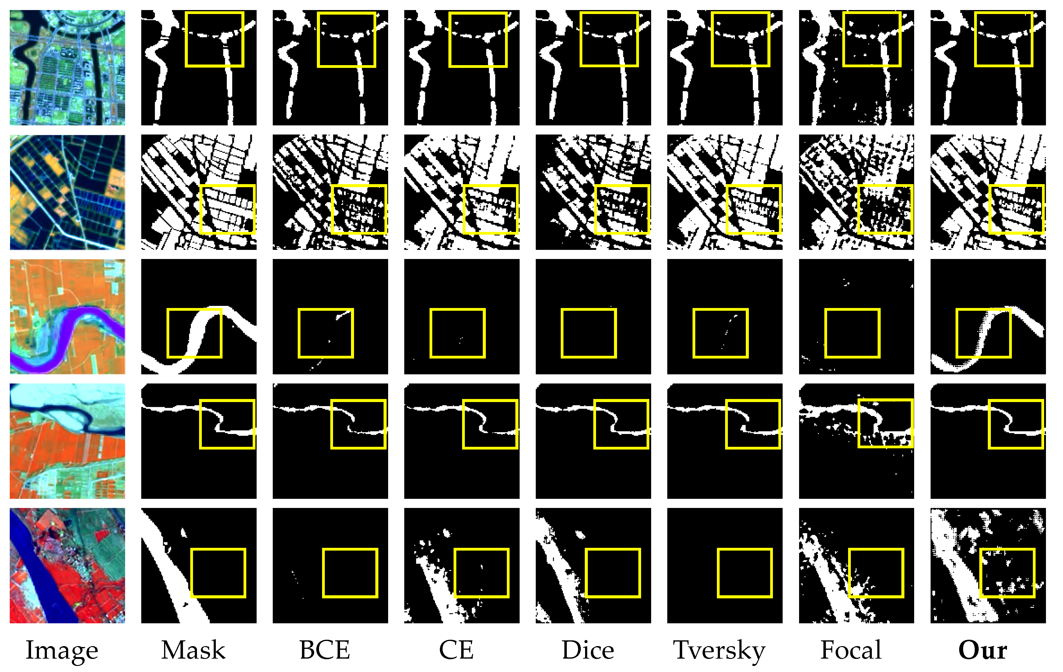
As shown in Figure 17, lines 1 and 2 show that SegNet employs Focal Loss to missegment shadows into bodies of water, but SegNet uses our loss function to segment the water bodies more effectively. As shown in lines 3 and 4 of Figure 17, SegNet captures more pixels of the water bodies using only our loss function. As shown in line 5 of Figure 17, SegNet did not identify the water bodies in the image using BCE Loss and Tversky Loss, and the other methods identified water body pixels with missed scores, but SegNet identified more details of water bodies using our loss function.

3.4. Discussion

In this study, from the experimental results in Section 3.1, the remote sensing water segmentation provided by our proposed approach is the most effective and makes full use of multi-scale features. Dense blocks can improve the use of features, and the MSPP gives the decoder additional spatial information on shallow features so that the relationship between pixels and masks may be precisely described, resulting in the best water-body segmentation. We also analyzed the water segmentation performance of DUPnet on two datasets: the LR dataset and the 2020 Gaofen challenge water body segmentation dataset. We found 16 mislabeled images in the LR dataset, which are shown on our publicly available website (https://github.com/xuemeichen99/DUPnet-Pytorch, accessed on 3 November 2022). These mislabeled data represent 0.22% of the total dataset. Most of the mislabeling images are located at the mixing area of water bodies and land, which makes it difficult for the human eyes to distinguish. This problem also exists for the Gaofen Challenge 2020 water body segmentation dataset with masks. Furthermore, the compute gradients are normalized at each iteration with RMSprop of the optimization algorithm, which helps reduce the impact of mis-masked samples. From the experimental results in Section 3.2, some representative cases demonstrate the capability of the proposed DUPnet method and other methods in identifying tributaries and watersheds at different scales. We used the MSPP as skip connections in the DUP network to collect multi-scale spatial domain information from remote sensing images. The MSPP can extract multi-scale features from the encoder layer’s down-sampling output, which has shallow layers and excellent feature resolution. The network can maintain more high-resolution detail information embedded in the high-level feature maps by fusing the multi-scale features with the decoder’s high-level features, thus improving image segmentation accuracy. The proposed DUPnet has the highest F1, MIoU, and FWIoU on the LR dataset and the 2020 Gaofen challenge water body segmentation dataset. From the results in Figure 12 and Figure 13, DUPnet provides a superior segmentation effect and retains the most water body information, particularly when extraction water fields narrow rivers. In addition, we proposed a loss function called LCTLoss and conducted a comparative analysis of different loss functions based on the experimental results in Section 3.3. As shown in Table 8 and Figure 14, Figure 15, Figure 16 and Figure 17, the result with LCTLoss is better than those with other loss function methods.
To summarize, the DUPnet network created and designed in this study has the following advantages:
(1)
Strong capacity for feature extraction: The encoder and decoder rely heavily on DB modules, which improve the network’s ability to extract semantic picture characteristics and provide highly abstracted feature images.
(2)
Minor loss of feature specifics: The skip connection employs a multi-scale spatial pyramidal pooling MSPP based on Atrous Convolution to enhance the use of features and compensate for the loss of information.
(3)
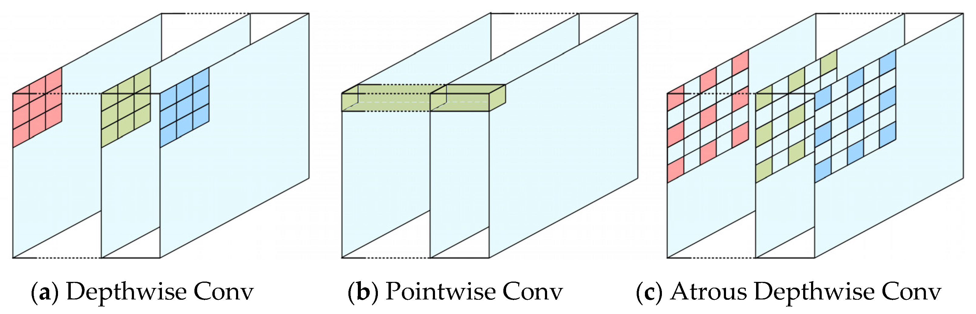
Large feature image perceptual field: Down-sampling module employs depth-separate convolution in replace of maximum pooling layer to enlarge the perceptual field of the feature map and enhance the robustness of the image features.

3.5. Limitations

Due to the limited spectral range of optical remote sensing images, the variety in water body shape and size, and the cloud coverage, water body masks for datasets may show a difference from the ground truth. Our proposed model also needs a high-quality dataset for training. However, there is a dearth of suitable datasets for supervised training in practice. Although incorporating a deep learning neural network model into the training and learning phase of remote sensing image recognition and extraction has the potential to better utilize image feature information, eliminate interference noise, and automate recognition and extraction, its accuracy is limited by the size and breadth of the training set. Future optimization of the model is also needed for training on more datasets.
To address some of the limitations, band combination could be used to reduce the background interference and help to more closely match the ground truth values. Other classifiers could also be used for dataset annotation to improve the accuracy and efficiency of dataset production. A dehaze model may also be developed to address the problem of cloud coverage on remote sensing images. Better model pruning and compressing mechanisms could also be investigated to further improving the performance of the proposed DUPnet model.

4. Conclusions

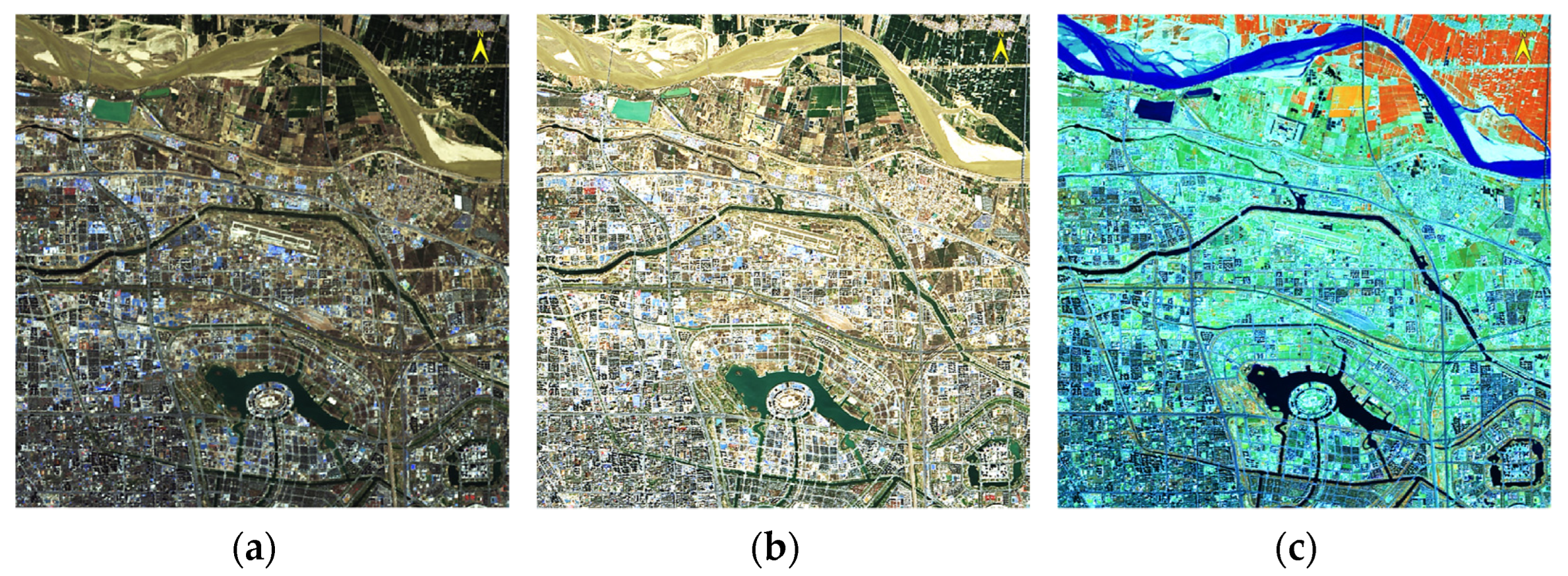
To improve the existing semantic segmentation algorithm of water bodies on remote sensing images and the limitations, a water body segmentation method based on dense blocks and the multi-scale pyramid pooling module (DUPnet) is proposed. We determined that the DUPnet can use the dense blocks to learn and propagate features, and the encoder part applies Atrous Separable Convolution (Sep Conv) down-sampling to increase the perceptual field of shallow feature maps and improve the robustness of image features. The skip connections can use the MSPP to extract multi-scale features of the encoder part layer to obtain multi-scale features. The up-sampling features are merged with multi-scale features in the decoder component, complementing the semantic and spatial information and boosting the decoder module’s images recovery capacity. A regression loss function based on Tversky coefficients and Log-Cosh regression is proposed in the deep learning model training, which can effectively improve the serious imbalance of positive and negative samples. In addition, we provide a fast method to generate datasets that can be used to train deep learning models. We selected the 5-6-4 bands combination of Landsat 8 OLI images to reduce the background interference. Then, we introduced ENVI SVM classifier for dataset annotation and two rounds of manual correction to improve the accuracy and efficiency of dataset production. This proved to provide good data support for extracting different types of water bodies in Landsat 8. This study efficiently resolves the technical problems of the inefficiency of water body sample masking, the difficulty of extracting small water bodies, the poor flexibility of extraction methods, and the lack of precision. The superiority of the proposed method for water segmentation on the 2020 Gaofen challenge water body segmentation dataset and the LR dataset is demonstrated in this study through ablation experiments and comparisons with comparable methods. DUPnet has the highest Precision, F1, MIoU, and FWIoU with values of 97.15%, 96.52%, 84.72%, and 91.77% on the LR dataset, respectively. On the 2020 Gaofen challenge water body segmentation dataset, DUPnet also has the highest F1, MIoU, and FWIoU with 97.67%, 88.17%, and 93.52%, respectively. To communicate with the researcher, the LR dataset has been provided online at https://github.com/xuemeichen99/DUPnet-Pytorch (accessed on 3 November 2022).
SVM classifiers can decrease the time and labor of annotation; however, they are generally very sensitive to the selection of appropriate kernel functions and parameter settings in remote sensing segmentation [49]. The superb fitting ability and portability of deep learning special have made the field of deep learning image algorithms highly popular. The combination of deep learning and machine learning methods will continue to be actively explored. For the dataset, we will continue to create larger, high-resolution multi-source datasets and find simpler and faster ways to improve the quality of the annotations. We will explore the weight assignment of the hybrid loss function in an adaptive manner. In addition, we will prune and compress the network to reduce the number of parameters as well as the processing time of the network while ensuring the performance of the model.

Author Contributions

Conceptualization, Z.L., X.C., S.Z., H.Y., J.G. and Y.L.; methodology, Z.L., X.C., S.Z. and Y.L.; validation, X.C., J.G. and H.Y.; formal analysis, X.C. and Y.L.; investigation, Z.L, X.C. and J.G.; writing—original draft preparation, Z.L. and X.C.; writing—review and editing, S.Z., J.G. and Y.L.; visualization, Z.L., H.Y. and J.G.; supervision, Y.L.; project administration, Z.L. and H.Y.; funding, Z.L. and H.Y. All authors have read and agreed to the published version of the manuscript.

Funding

This research was funded by the Fundamental Research Funds for the Central Universities under Grant XJS221307, JB211312.

Data Availability Statement

The code and Landsat River dataset will be available at https://github.com/xuemeichen99/DUPnet-Pytorch (accessed on 3 November 2022).

Conflicts of Interest

The authors declare no conflict of interest.

References

  1. Li, Y.; Dang, B.; Zhang, Y.; Du, Z. Water body classification from high-resolution optical remote sensing imagery: Achievements and perspectives. ISPRS J. Photogramm. Remote Sens. 2022, 187, 306–327. [Google Scholar] [CrossRef]
  2. Liu, J.; Wang, Y. Water Body Extraction in Remote Sensing Imagery Using Domain Adaptation-Based Network Embedding Selective Self-Attention and Multi-Scale Feature Fusion. Remote Sens. 2022, 14, 3538. [Google Scholar] [CrossRef]
  3. Yang, X.; Zhao, S.; Qin, X.; Zhao, N.; Liang, L. Mapping of Urban Surface Water Bodies from Sentinel-2 MSI Imagery at 10 m Resolution via NDWI-Based Image Sharpening. Remote Sens. 2017, 9, 596. [Google Scholar] [CrossRef] [Green Version]
  4. Chen, Y.; Fan, R.; Yang, X.; Wang, J.; Latif, A. Extraction of Urban Water Bodies from High-Resolution Remote-Sensing Imagery Using Deep Learning. Water 2018, 10, 585. [Google Scholar] [CrossRef] [Green Version]
  5. Chen, C.; He, X.; Lu, Y.; Chu, Y. Application of Landsat Time-Series Data in Island Ecological Environment Monitoring: A Case Study of Zhoushan Islands, China. J. Coastal Res. 2020, 108, 193–199. [Google Scholar] [CrossRef]
  6. McFeeters, S. The Use of Normalized Difference Water Index (NDWI) in the Delineation of Open Water Features. Int. J. Remote Sens. 1996, 17, 1425–1432. [Google Scholar] [CrossRef]
  7. Xu, H. Modification of Normalized Difference Water Index (NDWI) to Enhance Open Water Features in Remotely Sensed Imagery. Int. J. Remote Sens. 2006, 27, 3025–3033. [Google Scholar] [CrossRef]
  8. Cao, M.; Mao, K.; Shen, X.; Xu, T.; Yan, Y.; Yuan, Z. Monitoring the Spatial and Temporal Variations in The Water Surface and Floating Algal Bloom Areas in Dongting Lake Using a Long-Term MODIS Image Time Series. Remote Sens. 2020, 12, 3622. [Google Scholar] [CrossRef]
  9. Razaque, A.; Ben Haj Frej, M.; Almi’ani, M.; Alotaibi, M.; Alotaibi, B. Improved Support Vector Machine Enabled Radial Basis Function and Linear Variants for Remote Sensing Image Classification. Sensors 2021, 21, 4431. [Google Scholar] [CrossRef]
  10. Shetty, S.; Gupta, P.K.; Belgiu, M.; Srivastav, S.K. Assessing the Effect of Training Sampling Design on the Performance of Machine Learning Classifiers for Land Cover Mapping Using Multi-Temporal Remote Sensing Data and Google Earth Engine. Remote Sens. 2021, 13, 1433. [Google Scholar] [CrossRef]
  11. Li, A.; Fan, M.; Qin, G.; Xu, Y.; Wang, H. Comparative Analysis of Machine Learning Algorithms in Automatic Identification and Extraction of Water Boundaries. Applied Sciences 2021, 11, 10062. [Google Scholar] [CrossRef]
  12. Acharya, T.; Subedi, A.; Lee, D. Evaluation of Machine Learning Algorithms for Surface Water Extraction in a Landsat 8 Scene of Nepal. Sensors 2019, 19, 2769. [Google Scholar] [CrossRef] [Green Version]
  13. Miao, Z.; Fu, K.; Sun, H.; Sun, X.; Yan, M. Automatic Water-Body Segmentation from High-Resolution Satellite Images via Deep Networks. IEEE Geosci. Remote Sens. Lett. 2018, 15, 602–606. [Google Scholar] [CrossRef]
  14. Ronneberger, O.; Fischer, P.; Brox, T. U-Net: Convolutional Networks for Biomedical Image Segmentation. Proc 18th Int. Conf. Med. Image Comput. Comput.-Assist. Intervent 2015, 9351, 234–241. [Google Scholar]
  15. Chen, L.-C.; Zhu, Y.; Papandreou, G.; Schroff, F.; Adam, H. Encoder-Decoder with Atrous Separable Convolution for Semantic Image Segmentation. Proc. Eur. Conf. Comput. Vis. 2018, 833–851. [Google Scholar]
  16. Luo, X.; Tong, X.; Hu, Z. An applicable and automatic method for earth surface water mapping based on multispectral images. Int. J. Appl. Earth Obs. Geoinf. 2021, 103, 102472. [Google Scholar] [CrossRef]
  17. He, H.; Huang, X.; Li, H.; Ni, L.; Wang, X.; Chen, C.; Liu, Z. Water Body Extraction of High Resolution Remote Sensing Image based on Improved U-Net Network. J. Geo-Inf. Sci. 2020, 22, 2010–2022. [Google Scholar]
  18. Shelhamer, E.; Long, J.; Darrell, T. Fully Convolutional Networks for Semantic Segmentation. IEEE Trans. Pattern Anal. Mach. Intell. 2016, 39, 3431. [Google Scholar] [CrossRef]
  19. Badrinarayanan, V.; Kendall, A.; Cipolla, R. SegNet: A Deep Convolutional Encoder-Decoder Architecture for Image Segmentation. IEEE Trans. Pattern Anal. Mach. Intell. 2015, 39, 2481–2495. [Google Scholar] [CrossRef]
  20. Lin, G.; Milan, A.; Shen, C.; Reid, I. RefineNet: Multi-path Refinement Networks for High-Resolution Semantic Segmentation. In Proceedings of the IEEE Conference on Computer Vision and Pattern Recognition, Honolulu, HI, USA, 21–26 July 2017; pp. 5168–5177. [Google Scholar]
  21. Zhao, H.; Shi, J.; Qi, X.; Wang, X.; Jia, J. Pyramid Scene Parsing Network. In Proceedings of the IEEE Conference on Computer Vision and Pattern Recognition, Honolulu, HI, USA, 21–26 July 2017; pp. 6230–6239. [Google Scholar]
  22. Chen, L.-C.; Papandreou, G.; Kokkinos, I.; Murphy, K.; Yuille, A.L. Semantic Image Segmentation with Deep Convolutional Nets and Fully Connected CRFs. arXiv 2014, arXiv:1412.7062. [Google Scholar]
  23. Chen, L.C.; Papandreou, G.; Kokkinos, I.; Murphy, K.; Yuille, A.L. DeepLab: Semantic Image Segmentation with Deep Convolutional Nets, Atrous Convolution, and Fully Connected CRFs. IEEE Trans. Pattern Anal. Mach. Intell. 2018, 40, 834–848. [Google Scholar] [CrossRef] [PubMed] [Green Version]
  24. Chen, Q.; Zheng, L.; Li, X.; Xu, C.; WU, Y.; Xie, D.; Liu, L. Water Body Extraction from High-Resolution Satellite Remote Sensing Images Based on Deep Learning. Geogr. Geo-Inf. Sci. 2019, 35, 43–49. [Google Scholar]
  25. Wang, J.; Ke, S.; Cheng, T.; Jiang, B.; Deng, C.; Zhao, Y.; Liu, D.; Mu, Y.; Tan, M.; Wang, X.; et al. Deep High-Resolution Representation Learning for Visual Recognition. IEEE Trans. Pattern Anal. Mach. Intell. 2020, 43, 3349–3364. [Google Scholar] [CrossRef] [PubMed] [Green Version]
  26. Yin, Y.; Guo, Y.; Deng, L.; Chai, B. Improved PSPNet-based water shoreline detection in complex inland river scenarios. Complex Intell. Syst. 2022, 1–13. [Google Scholar] [CrossRef]
  27. Huang, G.; Liu, Z.; van der Maaten, L.; Weinberger, K. Densely Connected Convolutional Networks. In Proceedings of the IEEE Conference on Computer Vision and Pattern Recognition, Honolulu, HI, USA, 21–26 July 2017. [Google Scholar]
  28. Jadon, S. A survey of loss functions for semantic segmentation. In Proceedings of the IEEE Conference on Computational Intelligence in Bioinformatics and Computational Biology, CIBCB, Vina del Mar, Chile, 27–29 October 2020; pp. 1–7. [Google Scholar]
  29. Pihur, V.; Datta, S.; Datta, S. Weighted rank aggregation of cluster validation measures: A Monte Carlo cross-entropy approach. Bioinformatics 2007, 23, 1607–1615. [Google Scholar] [CrossRef] [PubMed]
  30. Lin, T.-Y.; Goyal, P.; Girshick, R.; He, K.; Dollár, P. Focal Loss for Dense Object Detection. Available online: https://arxiv.org/abs/1708.02002 (accessed on 14 September 2022).
  31. Sudre, C.H.; Li, W.; Vercauteren, T.; Ourselin, S.; Jorge Cardoso, M. Generalised Dice Overlap as a Deep Learning Loss Function for Highly Unbalanced Segmentations. Deep Learn Med. Image Anal. Multimodal. Learn Clin. Decis. Support 2017, 2017, 240–248. [Google Scholar]
  32. Abraham, N.; Khan, N.M. A Novel Focal Tversky Loss Function With Improved Attention U-Net for Lesion Segmentation. In Proceedings of the 2019 IEEE 16th International Symposium on Biomedical Imaging, Venice, Italy, 8–11 April 2019; pp. 683–687. [Google Scholar]
  33. Hashemi, S.R.; Salehi, S.S.; Erdogmus, D.; Prabhu, S.; Warfield, S.; Gholipour, A. Asymmetric Loss Functions and Deep Densely Connected Networks for Highly Imbalanced Medical Image Segmentation: Application to Multiple Sclerosis Lesion Detection. IEEE Access 2018, 7, 1721–1735. [Google Scholar] [CrossRef] [PubMed]
  34. Hayder, Z.; He, X.; Salzmann, M. Shape-aware Instance Segmentation. Available online: https://arxiv.org/abs/1612.03129v1 (accessed on 14 September 2022).
  35. Taghanaki, S.; Zheng, Y.; Zhou, S.K.; Georgescu, B.; Sharma, P.; Xu, D.; Comaniciu, D.; Hamarneh, G. Combo Loss: Handling Input and Output Imbalance in Multi-Organ Segmentation. Comput. Med. Imaging Graphics 2019, 75, 24–33. [Google Scholar] [CrossRef] [PubMed] [Green Version]
  36. Wong, K.; Moradi, M.; Tang, H.; Syeda-Mahmood, T. 3D Segmentation with Exponential Logarithmic Loss for Highly Unbalanced Object Sizes. In Proceedings of the MICCAI 2018, Granada, Spain, 16–20 September 2018; pp. 612–619. [Google Scholar]
  37. Yi-de, M.; Qing, L.; Zhi-bai, Q. Automated image segmentation using improved PCNN model based on cross-entropy. In Proceedings of the International Symposium on Intelligent Multimedia, Video and Speech Processing, Hong Kong, China, 20–22 October 2004; pp. 743–746. [Google Scholar]
  38. Sadegh, S.; Salehi, M.; Erdogmus, D.; Gholipour, A. Tversky Loss Function for Image Segmentation Using 3D Fully Convolutional Deep Networks. Available online: https://arxiv.org/abs/1706.05721v1 (accessed on 14 September 2022).
  39. Szegedy, S.I.a.C. Batch normalization: Accelerating deep network training by reducing internal covariate shift. In Proceedings of the 32nd International Conference on Machine Learning ICML, Lile, France, 6–11 July 2015; pp. 448–456. [Google Scholar]
  40. Glorot, X.; Bordes, A.; Bengio, Y. Deep Sparse Rectifier Neural Networks. In Proceedings of the 14th International Conference on Artificial Intelligence and Statistics AISTATS, Fort Lauderdale, FL, USA, 11–13 April 2011; pp. 315–323. [Google Scholar]
  41. Chollet, F. Xception: Deep Learning with Depthwise Separable Convolutions. In Proceedings of the IEEE Conference on Computer Vision and Pattern Recognition, Honolulu, HI, USA, 21–26 July 2017; pp. 1800–1807. [Google Scholar]
  42. Huk, M. Stochastic Optimization of Contextual Neural Networks with RMSprop. In Intelligent Information and Database Systems; Springer: Cham, Switzerland, 2020; pp. 343–352. [Google Scholar]
  43. Liu, W.; Rabinovich, A.; Berg, A.C. Parsenet: Looking Wider to See Better. Available online: https://arxiv.org/abs/1506.04579 (accessed on 14 September 2022).
  44. Sun, X.; Wang, P.; Yan, Z.; Diao, W.; Lu, X.; Yang, Z.; Zhang, Y.; Xiang, D.; Yan, C.; Guo, J.; et al. Automated High-Resolution Earth Observation Image Interpretation: Outcome of the 2020 Gaofen Challenge. IEEE J. Sel. Top. Appl. Earth Obs. Remote Sens. 2021, 14, 8922–8940. [Google Scholar] [CrossRef]
  45. ENVI. Available online: https://www.l3harrisgeospatial.com/Software-Technology/ENVI (accessed on 16 October 2022).
  46. Jat, M.; Garg, P.; Dahiya, S. A comparative study of various pixel based image fusion techniques as applied to an urban environment. Int. J. Image Data Fusion 2013, 4, 197–213. [Google Scholar]
  47. Cortes, C.; Vapnik, V. Support-vector networks. Chem. Biol. Drug Des. 2009, 297, 273–297. [Google Scholar] [CrossRef]
  48. Mountrakis, G.; Im, J.; Ogole, C. Support vector machines in remote sensing: A review. ISPRS J. Photogramm. Remote Sens. 2011, 66, 247–259. [Google Scholar] [CrossRef]
  49. Maulik, U.; Chakraborty, D. Remote Sensing Image Classification: A survey of support-vector-machine-based advanced techniques. IEEE Geosci. Remote Sens. Mag. 2017, 5, 33–52. [Google Scholar] [CrossRef]
  50. Cilli, R.; Monaco, A.; Amoroso, N.; Tateo, A.; Tangaro, S.; Bellotti, R. Machine Learning for Cloud Detection of Globally Distributed Sentinel-2 Images. Remote Sens. 2020, 12, 2355. [Google Scholar] [CrossRef]
  51. ENVISVMClassifier. Available online: https://www.l3harrisgeospatial.com/docs/ENVISVMClassifier.html (accessed on 16 October 2022).
  52. Lee, C.-Y.; Xie, S.; Gallagher, P.; Zhang, Z.; Tu, Z. Deeply-Supervised Nets. Available online: https://arxiv.org/abs/1409.5185 (accessed on 14 September 2022).
  53. Simonyan, K.; Zisserman, A. Very Deep Convolutional Networks for Large-Scale Image Recognition. Available online: https://arxiv.org/abs/1409.1556 (accessed on 14 September 2022).
  54. Gedraite, E.S.; Hadad, M. Investigation on the effect of a Gaussian Blur in image filtering and segmentation. In Proceedings of the ELMAR-2011, Zadar, Croatia, 14–16 September 2011; pp. 393–396. [Google Scholar]
  55. Etzkorn, B. Data Normalization and Standardization. Available online: https://www.geeksforgeeks.org/normalization-vs-standardization/ (accessed on 14 September 2022).
  56. Zhang, P.; Xu, C.; Ma, S.; Shao, X.; Tian, Y.; Wen, B. Automatic Extraction of Seismic Landslides in Large Areas with Complex Environments Based on Deep Learning: An Example of the 2018 Iburi Earthquake, Japan. Remote Sens. 2020, 12, 3992. [Google Scholar] [CrossRef]
  57. Sisodia, P.S.; Tiwari, V.; Kumar, A. Analysis of supervised maximum likelihood classification for remote sensing image. In Proceedings of the International Conference on Recent Advances and Innovations in Engineering (ICRAIE-2014), Jaipur, India, 9–11 May 2014; pp. 1–4. [Google Scholar]
  58. Xie, S.; Tu, Z. Holistically-Nested Edge Detection. Int. J. Comput. Vision 2017, 125, 1–16. [Google Scholar] [CrossRef]
Figure 1. The DUP network structure diagram.
Remotesensing 14 05567 g001
Figure 2. The dense block (DB) in DUPnet, l is 4, and the growth rate is 24.
Remotesensing 14 05567 g002
Figure 3. (a) The MSPP, which serves to fuse multi-scale shallow features with deep features. (b) Down-sampling (Down) Module.
Remotesensing 14 05567 g003
Figure 4. (a) 3 × 3 depth convolution is spatial convolution on each channel alone; (b) point-by-point convolution is a combination of depth convolution using 1 × 1 convolution kernels to obtain features; (c) 3 × 3 Atrous Separable Convolution with rate of 2 is a combination of Atrous Convolution and depth convolution to increase the perceptual field of the convolution.
Remotesensing 14 05567 g004
Figure 5. Qualitative segmentation examples from the 2020 Gaofen challenge water body segmentation dataset (left two) and the LR dataset (right two).
Remotesensing 14 05567 g005
Figure 6. Raw remote sensing images are preprocessed to produce (a) brovey transformed image, (b) corrected image, and (c) false color composite image.
Remotesensing 14 05567 g006
Figure 7. Visualization of extraction results of water bodies for ablation studies on the 2020 Gaofen challenge water body segmentation dataset.
Remotesensing 14 05567 g007
Figure 8. Visualization of extraction results of small water bodies for ablation studies on the 2020 Gaofen challenge water body segmentation dataset.
Remotesensing 14 05567 g008
Figure 9. The histogram of quantitative comparison of different models in terms of Accuracy, Precision, and Recall (%) on the LR dataset.
Remotesensing 14 05567 g009
Figure 10. The histogram of quantitative comparison of different models in terms of F1, MIoU, and FWIoU (%) on the 2020 Gaofen challenge water body segmentation dataset and the LR dataset.
Remotesensing 14 05567 g010
Figure 11. ROC and P–R curves for evaluating the ability of different models to segment water on the LR dataset. (a) ROC curves for evaluating different models on water body segmentation, (b) P-R curves for evaluating different models on water body segmentation.
Remotesensing 14 05567 g011
Figure 12. Qualitative evaluation with state-of-the-art methods on the 2020 Gaofen challenge water body segmentation dataset and the LR dataset.
Remotesensing 14 05567 g012
Figure 13. Qualitative evaluation with state-of-the-art methods in small bodies of water on the 2020 Gaofen challenge water body segmentation dataset and the LR dataset.
Remotesensing 14 05567 g013aRemotesensing 14 05567 g013b
Figure 14. The histogram of various loss functions on network performance metric (%).
Remotesensing 14 05567 g014
Figure 15. ROC and P–R curves to evaluate the ability of U-Net (a,b) and SegNet (c,d) to segment the water column using different loss functions.
Remotesensing 14 05567 g015aRemotesensing 14 05567 g015b
Figure 16. Example of U-Net network segmenting water bodies using 6 different loss functions.
Remotesensing 14 05567 g016aRemotesensing 14 05567 g016b
Figure 17. Example of SegNet network segmenting water bodies using 6 different loss functions.
Remotesensing 14 05567 g017
Table 1. Parameter settings for each layer in the DUPnet network.
LayersInput ShapeOutput ShapeStructure
Conv 0(3, 128, 128)(64, 128, 128)3 × 3 Conv + BN + ReLU
3 × 3 Conv + BN + ReLU
DB 1(64, 128, 128)(160, 128, 128) [ 1 × 1 C onv + B N + Re L U 3 × 3 C onv + B N + Re L U ] × 4
Down 1(160, 128, 128)(256, 64, 64)3 × 3 Sep conv, stride 2
DB 2(256, 64, 64)(352, 64, 64) [ 1 × 1 C onv + B N + Re L U 3 × 3 C onv + B N + Re L U ] × 4
Down 2(352, 64, 64)(512, 32, 32)3 × 3 Sep conv, stride 2
DB 3(512, 32, 32)(608, 32, 32) [ 1 × 1 C onv + B N + Re L U 3 × 3 C onv + B N + Re L U ] × 4
Down 3(608, 32, 32)(1024, 16, 16)3 × 3 Sep conv, stride 2
DB 4(1024, 16, 16)(1120, 16, 16) [ 1 × 1 C onv + B N + Re L U 3 × 3 C onv + B N + Re L U ] × 4
Down 4(1120, 16, 16)(1120, 8, 8)3 × 3 Sep conv, stride 2
DB 5(1120, 8, 8)(1216, 8, 8) [ 1 × 1 C onv + B N + Re L U 3 × 3 C onv + B N + Re L U ] × 4
Up 1(1216, 8, 8)(1216, 16, 16)up-sampling
(1216, 16, 16)(608, 16, 16)1 × 1 Conv + BN + ReLU
DB 6(608, 16, 16)(704, 16, 16) [ 1 × 1 C onv + B N + Re L U 3 × 3 C onv + B N + Re L U ] × 4
Up 2(704, 16, 16)(704, 32, 32)up-sampling
(704, 32, 32)(352, 32, 32)1 × 1 Conv + BN + ReLU
DB 7(352, 32, 32)(448, 32, 32) [ 1 × 1 C onv + B N + Re L U 3 × 3 C onv + B N + Re L U ] × 4
Up 3(448, 32, 32)(448, 64, 64)up-sampling
(448, 64, 64)(224, 64, 64)1 × 1 Conv + BN + ReLU
DB 8(224, 64, 64)(320, 64, 64) [ 1 × 1 C onv + B N + Re L U 3 × 3 C onv + B N + Re L U ] × 4
Up 4(320, 64, 64)(320, 128, 128)up-sampling
(320, 128, 128)(160, 128, 128)1 × 1 Conv + BN + ReLU
DB 9(160, 128, 128)(256, 128, 128) [ 1 × 1 C onv + B N + Re L U 3 × 3 C onv + B N + Re L U ] × 4
Classification Layer(256, 128, 128)(128, 128, 128)3 × 3 conv + BN + ReLU
(128, 128, 128)(128, 128, 128)3 × 3 conv + BN + ReLU
(128, 128, 128)(2, 128, 128)1 × 1 conv + BN + ReLU
Table 2. Image data were utilized to classify the research area.
Date AcquiredPath/RowSun Azimuth (°)Sun Elevation (°)Cloud Cover (%)Resolution (m)
2021/03/22124/36142.71149.8440.0530
2021/08/02127/32134.45860.7910.0530
2021/09/12126/37142.20655.1980.0330
Table 3. Comparison of F1, MIoU, and FWIoU with the different dilation rates (%) on the 2020 Gaofen challenge water body segmentation dataset.
Dilation RateF1MIoUFWIoU
{1, 6, 9, 12} 91.2272.3778.23
{1, 6, 12, 18} 92.8576.3781.78
{1, 12, 24, 36} 91.9573.9179.79
Table 4. Quantitative comparison of ablation study in terms of F1, MIoU, and FWIoU (%) on the 2020 Gaofen challenge water body segmentation dataset. Symbol (√) means this part/module is selected to be used in the original U-Net.
MethodMSPPDBF1MIoUFWIoU
U-Net 91.6573.6878.99
U-Net 92.8576.37 81.78
U-Net 91.3273.8577.40
DUPnet93.4978.6483.46
Table 5. Quantitative comparison of different models in terms of Accuracy, Recall, and Precision (%) on the LR dataset.
ModelsBackboneAccuracyRecallPrecision
FCN [18]ResNet-5087.5596.1986.60
U-Net [14]-90.2397.6289.69
SegNet [19]-90.3091.9694.67
PSPNet [21]ResNet-5085.5095.6984.25
DeeplabV3+ [15]ResNet-5089.1597.0087.64
ENVINet5 [56]-99.4985.4454.59
MLC [57]-99.8277.9291.03
HRNet V2 [25]-87.1796.9286.00
DUPnet-95.4096.1697.15
Table 6. Quantitative comparison of different models in terms of F1, MIoU, and FWIoU (%) on the 2020 Gaofen challenge water body segmentation dataset and the LR dataset.
2020 Gaofen Challenge Water Body Segmentation Dataset LR Dataset
ModelsF1MIoUFWIoUF1MIoUFWIoU
FCN96.3180.5189.5190.0070.0681.67
U-Net97.2485.6492.2292.6778.3785.85
SegNet92.7162.2379.7993.0068.7183.74
PSPNet96.3980.5689.8488.0566.0779.04
DeeplabV3+96.9583.6191.3391.3072.6383.58
ENVINet592.7461.5379.5166.6149.9457.70
MLC94.3174.4385.0083.9772.3683.93
HRNet V296.8983.9291.2089.6070.7181.79
DUPnet97.6788.1793.5296.5284.7291.77
Table 7. Comparison of spatial complexity and time with the latest models on the LR dataset.
ModelsModel Size (M)Times (s)
FCN2430.3056
U-Net1530.2500
SegNet3370.3333
PSPNet5340.5556
DeeplabV3+4710.4722
HRNet V21110.0900
DUPnet2960.4444
Table 8. The impact of various loss functions on network performance metric (%).
ModelLossAccuracyPrecisionRecallF1MIoUFWIoU
U-NetCE [37]89.9958.7485.0167.3970.6083.28
BCE [58]88.4898.1888.4192.3465.9580.64
Focal [30]88.6457.4977.2463.6967.7081.49
Dice [31]88.0292.6692.7791.7269.0281.51
Tversky [38]86.5297.8187.2691.3161.9477.87
Our90.2389.6997.6292.6778.3785.85
SegNetCE88.2961.9679.2659.8568.7781.43
BCE87.6099.2786.9891.9961.0378.93
Focal86.8657.8869.4162.8263.5779.90
Dice88.2897.1289.1892.1266.8680.84
Tversky87.7998.5387.8792.0463.6279.34
Our90.3094.6791.9693.0068.7183.74
Publisher’s Note: MDPI stays neutral with regard to jurisdictional claims in published maps and institutional affiliations.

