Communication

WaterMaskAnalyzer (WMA)—A User-Friendly Tool to Analyze and Visualize Temporal Dynamics of Inland Water Body Extents

1
Saxon State Ministry for Economic Affairs, Labour and Transport, 01097 Dresden, Germany
2
Saxon State Company for Environment and Agriculture, 01445 Radebeul, Germany
3
Saxon State Office for Environment, Agriculture and Geology, 01326 Dresden, Germany
*
Author to whom correspondence should be addressed.
Remote Sens. 2022, 14(18), 4485; https://doi.org/10.3390/rs14184485
Submission received: 20 July 2022 / Revised: 28 August 2022 / Accepted: 2 September 2022 / Published: 8 September 2022

Abstract

:
Freely available satellite imagery from the EU Copernicus program can record water surfaces precisely and at high temporal resolution. This paper provides the development status of the open-source demo software “WaterMaskAnalyzer” (WMA) for the determination of water body extents. The application allows simple to use on-demand monitoring of inland water dynamics by the Otsu-thresholding algorithm that automatically classifies water bodies. The tool can answer various hydrological issues related to disaster and water management, nature conservation, or water body monitoring. The first results from investigations of the Sentinel-1 time series in VH polarization show high accuracies with R2 = 0.824 compared to in situ measurements for the Quitzdorf reservoir in Saxony, Germany. Small or indented-shaped water bodies, as well as those with forested riparian zones, such as the Cranzahl (VH: R2 = 0.102 and VV: R2 = 0.251) and Klingenberg reservoirs (VH: R2 = 0.091 and VV: R2 = 0.146), only achieve a low R2 for VV and VH polarization but receive equally low RMSEs of 0.045 km2 (Cranzahl) and 0.077 km2 (Klingenberg). By separating out outliers and using correction factors, fast improvements in the accuracies can be expected. For future improvements, alternate classification methods and diverse new ground-truth data lead us to expect the next big step in development.

1. Introduction

Water bodies show permanent water level fluctuations. Both natural and artificial water share this characteristic. The monitoring of water body extents is of central importance for the investigation of many public health and ecological questions [1]. The knowledge of the extent and dynamics of running and standing water bodies is crucial for instant and future management. In addition, in situ lake level measurements are globally sparse [2]. By using freely available satellite data with high temporal and sufficient spatial resolution, the hydrological database can be considerably expanded and thus contribute to the fulfillment of official administrative tasks. The areas of application are diverse, from public health topics to extreme events, such as drought and floods [3]. Low water levels also have a negative impact on water quality, on which drinking water reservoirs and the population they supply are particularly dependent. In addition, knowledge of water availability during drought is important for answering ecological questions [4]. The review of the implementation of measures from the Common Agricultural Policy (CAP) is also based on knowledge of water levels (i.e., pond measures) [5]. Multitemporal data can be used specifically to visualize the water surface dynamics and extents of highly fluctuating inland water bodies and broader streams to monitor water management activities and extreme hydrological events. Also, for the identification of inundation areas for flood damage evaluation, the derivation of mean water levels and water–land borders are necessary, as well as determining water recurrence, the delineation of riparian zones, water exchange areas, and partly wetlands [3,4].
Great progress has been made at a global scale in mapping surface water and its long-term changes [6]. By using more than three million images from several Landsat missions, the authors are mapping months and years when water was present over the past 36 years with their tool, Global Surface Water Explorer (https://global-surface-water.appspot.com/) (accessed on 10 January 2022). Some investigation parameters are available as a web service and offer temporal profile charts for each location in the world [7] but allow only investigations of water bodies based on pre-processed data. The user has no influence on the investigation period, which always covers 1984 to 2020. Although the temporal profiles of individual pixels can be displayed, the dynamics of the entire water body cannot be recorded. Possibilities of data export do not exist. By using Sentinel-1 C-Band Synthetic Aperture Radar (SAR), there is great potential for the automated monitoring of short-time changes [8]. This imagery has a high spatial and temporal resolution, is unaffected by cloud cover, and fulfills the requirements for ideal monitoring of inland water dynamics. There is high potential for rapid mapping of water bodies at a large scale, high spatial resolution, and accuracy by using the powerful cloud-based processing platform Google Earth Engine (GEE) [9,10,11,12]. The first systems are already implemented that use Sentinel-1 data to evaluate inland water dynamics using GEE (e.g., “Sentinel-1 based Inland water dynamics Mapping System” (SIMS), https://sims-toolkit.herokuapp.com) (accessed on 30 May 2022) [13]. Here, too, the setting options by the user are limited.
Therefore, the aim of this work was to develop a simple-to-use on-demand monitoring tool for inland water dynamics using a robust and proven classifier on satellite images. The application concept of the WaterMaskAnalyzer (WMA) provides a flexible analysis of different types of satellite data with a universal processing algorithm to determine the water surface extent. The main purpose is to provide on-demand analyses and visualizations of temporal dynamics for inland water bodies along with the extraction of observed surface water extents in an easy-to-understand, modularly structured interface. With the validation using in situ data, the initial results for water surface mapping and calculation can be evaluated.
On the basis of the satellite image time series determined by the user (Sentinel-1 in VV or VH polarization, or the “Normalized Difference Water Index” (NDWI) calculated from Sentinel-2 or Landsat-8 bands), an individual water mask can be created. The result is a graduated representation of the temporal coverage of the pixels with water.
The WMA closes an important gap in demand-based water body mask generation and, in contrast to other systems, enables the processing of very individual and detailed questions. To ensure this individuality, the WMA should provide many functions: Free choice of the investigation area and the survey period, the satellite system, and, if possible, the associated polarizations, as well as other parameters such as filters or minimum mapping units. In addition, the WMA does not require the user to have their own processing resources for big data processing; as a cloud-based system, the WMA guarantees efficiency, resource-saving, and simple product generation.

2. Requirements, Materials and Methods

2.1. Web Tool Requirements

We identified eleven main requirements for a web tool working with remote sensing data: The results should (1) be provided without espouse time, and the calculations require (2) as little data input as possible from the user. As a web application, (3) the permanent availability of the service is desired. The application must be able to draw on (4) an extensive catalog of pre-processed satellite data to achieve large spatial coverage at high temporal resolution. This is currently possible, in particular, with data from the EU Copernicus program, which should also (5) provide weather-independent mapping through predestined SAR-image recordings. The (6) database should always be up-to-date. The use of approved scientific methods and algorithms should guarantee a (7) high quality of the results. The results are intended to show the relative proportion of the pixels that were covered with water during the study period, which highlights the dynamic areas in particular. The user should be provided with (8) easy-to-use tools and the possibility to perform (9) graphical and (10) statistical analyses and evaluations of individual scenes or entire time series. The user must also be able to (11) export results for further processing independently of the WMA.

2.2. Water Mask Extraction

2.2.1. Data Used

In general, the WMA supports the image segmentation of radar and optical satellite imagery. The application is currently designed to process Sentinel-1, Sentinel-2, and Landsat-8 datasets.
Regarding the satellite imagery used, the core focus is on Sentinel-1. Sentinel-1 consists of two satellites that were launched in 2014 (Sentinel-1A) and 2016 (Sentinel-1B) [10]. The first image, e.g., the Quitzdorf reservoir, was taken on 3 October 2014. Until October 2016, eight to ten images are available for Quitzdorf taken from ascending or descending orbit by Sentinel-1A. From November 2016 until the end of December 2021, about 20 images per month will then be available for the study area, as Sentinel-1B will now also provide images. The Sentinel-1B mission was completed in December 2021 due to a technical malfunction. The spatial resolution corresponds to a 10 × 10 m pixel size of the Sentinel-1 GRD product in IW mode [10].
To carry out the validation of the measurement results, official in situ data from the Federal Dam Administration of Saxony were used for the investigated reservoirs of Cranzahl, Klingenberg, and Quitzdorf [14]. The water-area data were derived from daily measurements of the water level in combination with a digital lake bottom and elevation model of the reservoirs.

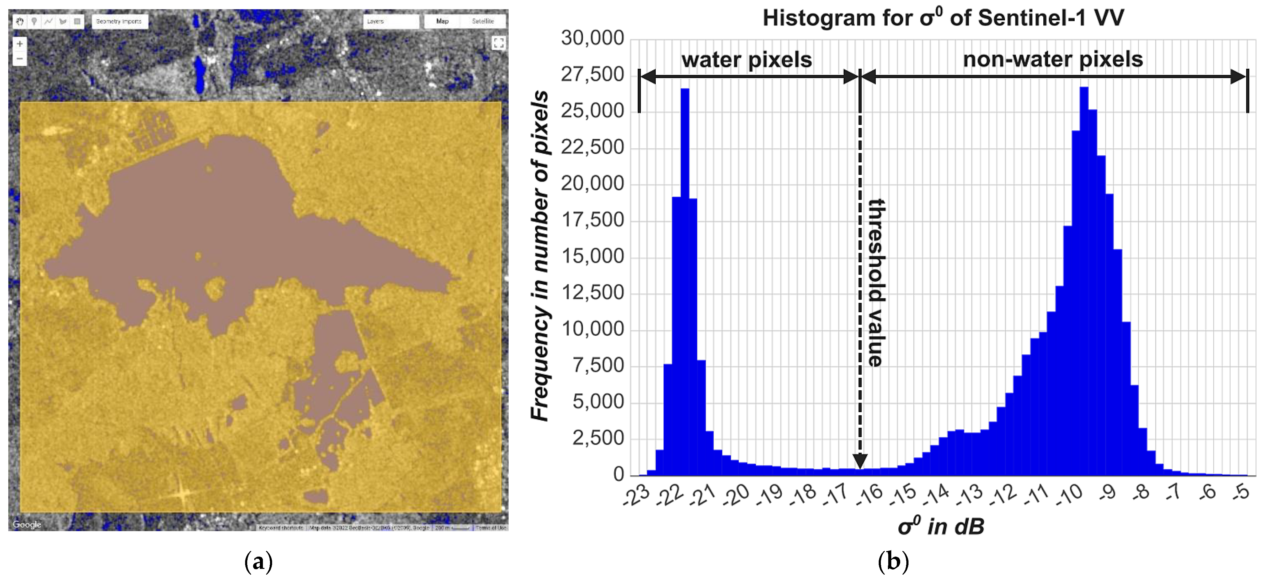
2.2.2. Classification Method

Varieties of methods are available today for classifying a land cover, such as a water surface from a satellite image. These range from data-driven machine learning methods [15,16] to statistical methods, such as threshold selection, according to Otsu [17]. The decision to use the Otsu method is because it is established for the intended classification with good results [18]. In addition, low computing capacities and little user interaction are required for implementation [18]. The user does not need any additional data apart from the geometry of the study area (Figure 1a) and does not have to determine any training areas, for example, which makes the application of the Otsu method very user-friendly and quickly ready for use. Dealing with 455 Sentinel-1-images in 2020, the WMA needs 3:30 min to create the final water mask of the Quitzdorf reservoir.
Otsu’s method [17], an automatic thresholding algorithm for the segmentation of digital images, splits the pixel values into two classes, in this case, water (where the pixel value = 1) and non-water (where the pixel value = 0). Figure 1b illustrates a histogram that shows the distribution of the pixel value classes and their frequency for an exemplary water body (a). Smooth surfaces, such as bodies of water, reflect the transmitted radar pulse away from the receiver. In the histogram in Figure 1b, this can be seen from the fact that the water pixels have lower backscatter values than the non-water pixels. When the pixel radar intensity or the backscatter coefficient (σ0) as the physical quantity equivalent is plotted on the histogram, two characteristic peaks emerge. Otsu’s method detects the optimal threshold near the local minimum between them. Based on the automated process, an individual value is calculated for every image to mask all water pixels below this limit.

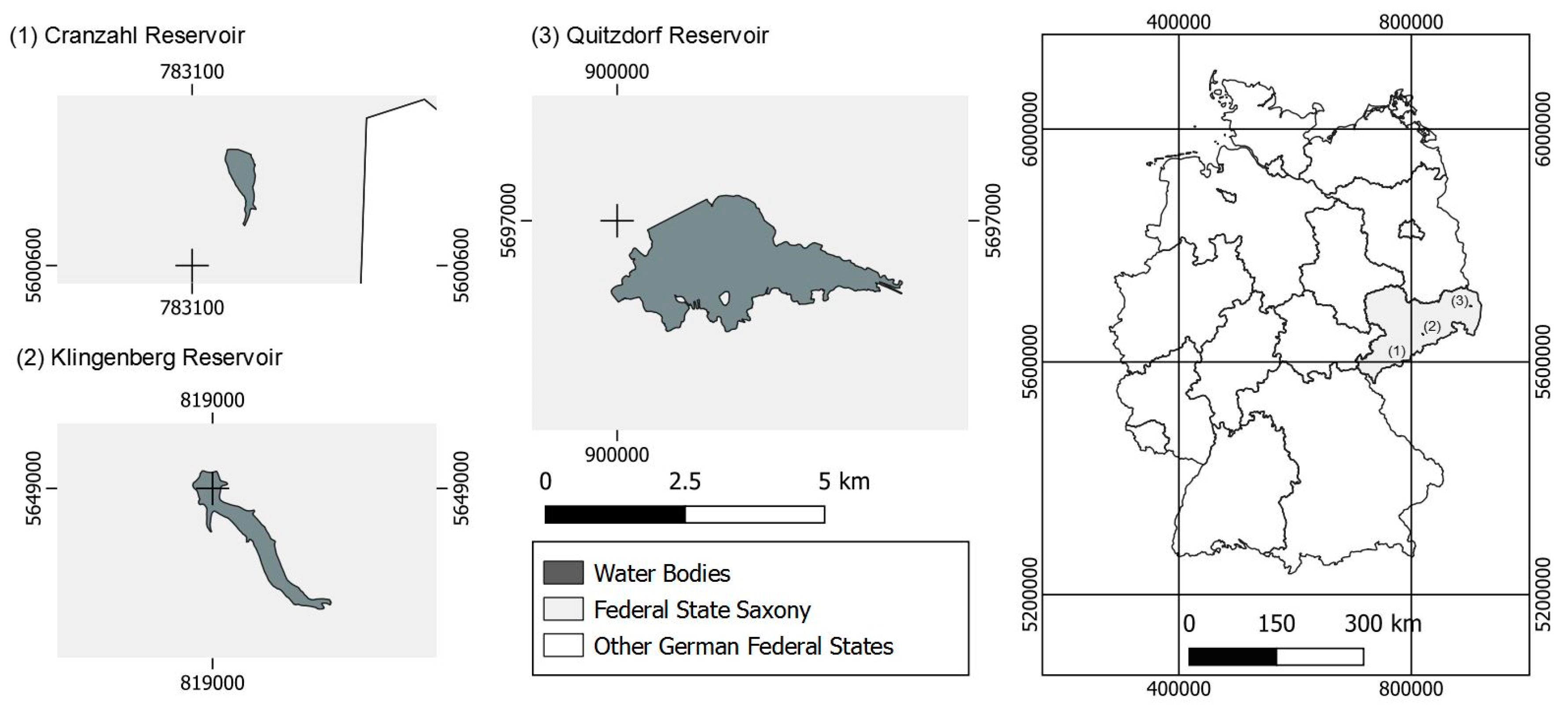
2.3. Investigation Area

To test the functionality of the WMA and the classification results, three representative water bodies in eastern Federal State Saxony, Germany, were selected (Figure 2). The Quitzdorf reservoir is located west of the Town of Niesky in the region of Upper Lusatia. With a maximum water surface of more than 6.66 km2 (with an operating space volume of 16.48 Mio. m3) in 2018, it is the largest reservoir in Saxony. Its main functions are the provision of service water, flood protection, and low water elevation. The Cranzahl reservoir (0.35 km2 and 2.85 Mio. m3) and the Klingenberg reservoir (1.16 km2 and 14.14 Mio. m3) are located in the Ore Mountains and are used to supply drinking water.
About three-quarters of the riparian zone of Cranzahl consists of coniferous forests. The remaining shares are distributed among mixed forests, mixed deciduous forests, and grassland. Mainly the riparian zone of Klingenberg is lined by coniferous forests, followed by mixed forests. The riparian zone of Quitzdorf is predominantly dominated by riverine vegetation (reeds and copses).
In the drinking water dams, Cranzahl and Klingenberg, the water level is mainly influenced by the inflowing water, which is why events such as drought have a particular impact here. Since Quitzdorf also serves as flood protection, the water level is managed even more actively here. Thus, reservoir space (4.45 Mio. m3) is kept available to counteract heavy precipitation events [14].

3. Results

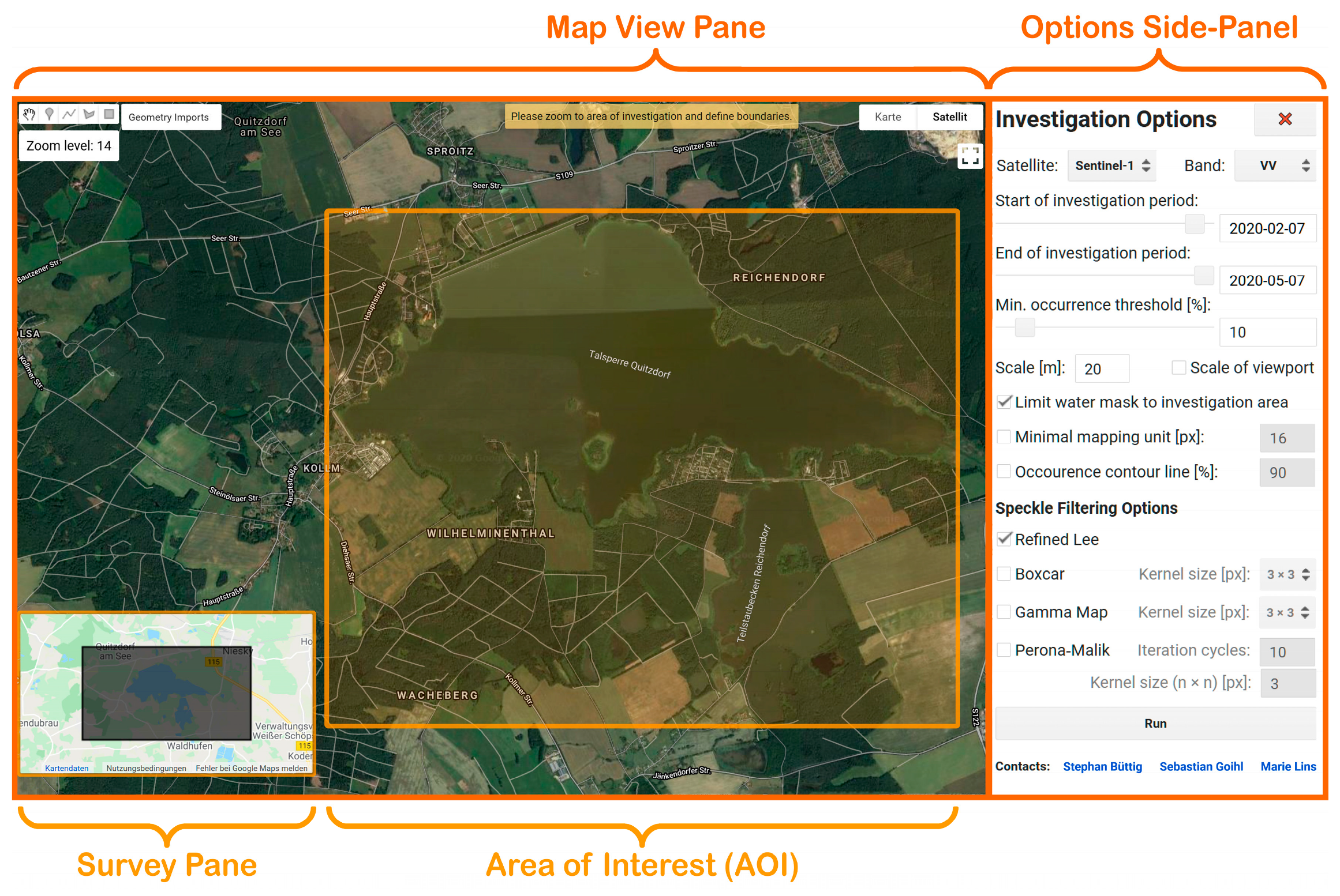
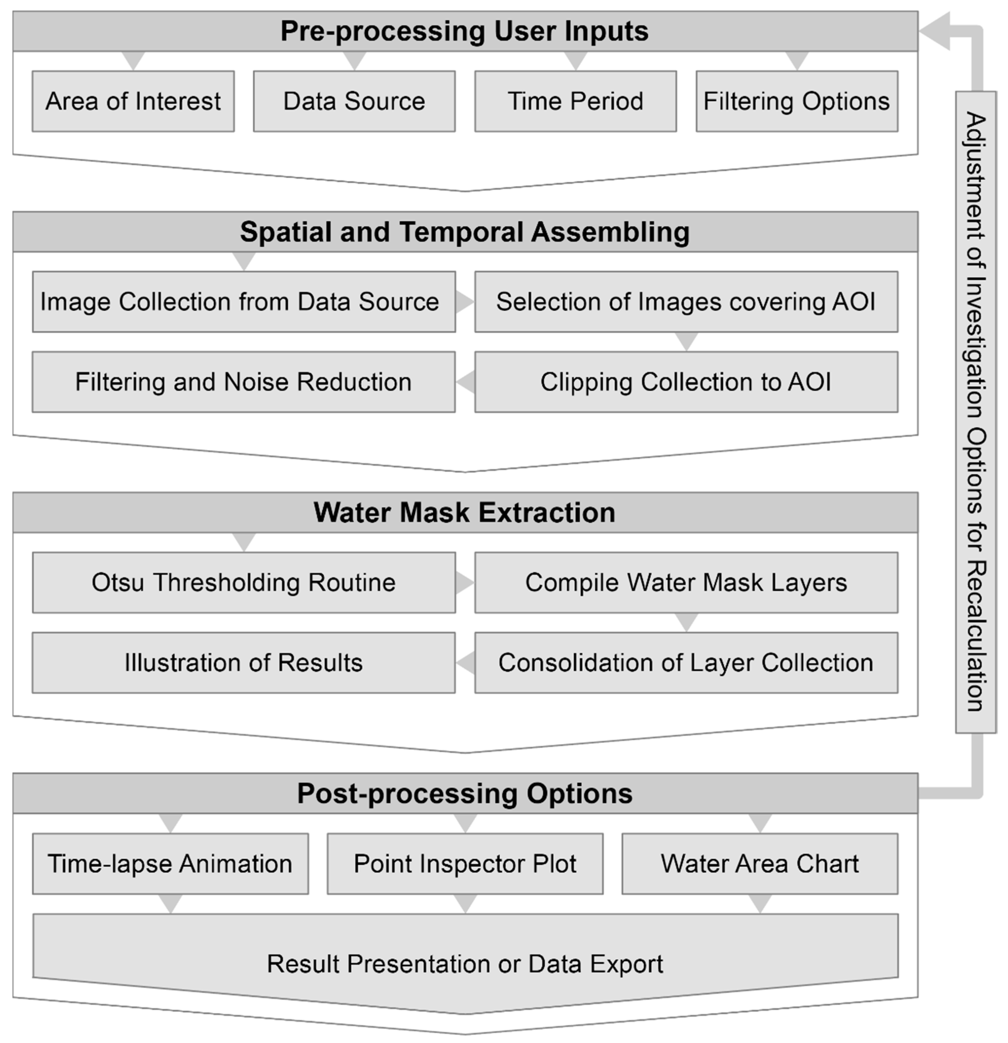
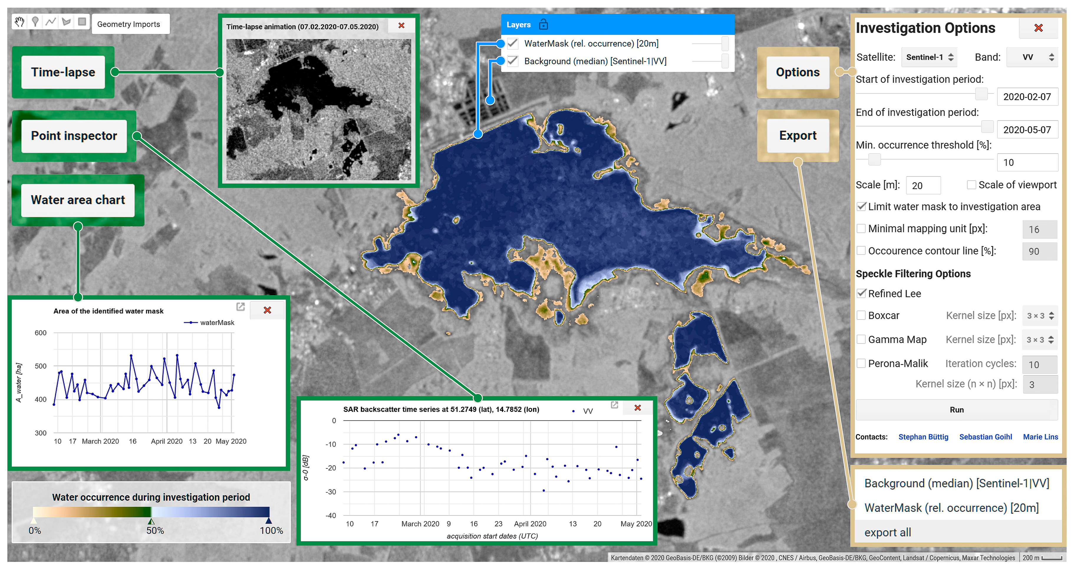
3.1. Web Tool Development

The requirements for the WMA as a web tool and the processing methods described in Section 2.1 and Section 2.2 could be successfully implemented by using GEE. This web-based online demo application is available at https://bit.ly/3wEdnMI (accessed on 19 July 2022).
After launching the application, the initial map view (Figure 3) is used to define the area of interest (AOI) with a geometry tool. Analyzing an extensive collection of satellite scenes makes it necessary to first reduce or customize the dataset depending on the relevant study area (the AOI) and time period. This includes spatial and temporal assembling with convenient methods for clipping or filtering [19]. The pre-processed Sentinel and Landsat datasets already contain basic radiometric and atmospheric corrections. To avoid any misrepresentation, truncated or partial satellite images that do not fully cover the area of interest (AOI) are filtered out. This also involves optical satellite imagery with adverse cloud coverage, which can be automatically sorted out by an adjustable filter function. The full processing scheme is shown in Figure 4.
The WMA offers various adjustments, analyzing as well as export functions that are embedded in a modularly structured and flexibly expandable interface. These can be handled through control elements in an adapted pre- and post-processing user interface.
The main segmentation processing (Figure 4) uses Otsu’s method to mask the water surface in each image of the investigation period, summed pixel-wise and divided by the number of the processed images. As a result, a consolidated layer is generated that illustrates the water occurrence in percentages between 0% and 100%. To reduce granular noise in the radar data from the interference of waves reflected from elementary scatterers [18], several standard speckle-filtering techniques are available. In comparison, multispectral imagery tends to have considerably less noisy scenes, so there is a simple smoothing option in the WMA to blur uneven texture.
The results are summarized as different stacked output layers in the WMA post-processing map view. The background layer represents a reduction of all available satellite images by calculating the median for each pixel across the entire collection of the investigation period. The calculated water occurrence layer is shown at the top level, which illustrates areas that were never (0%) up to constantly (100%) covered with water as a natural color gradient. For better delineation, the contour of the water surface can also be displayed for any of these percentage values.
The post-processing map view (Figure 5) offers additional analyzing tools. The time-lapse function creates an animation from a series of satellite images available in a specific period. By calling the point inspector, a time series of the thresholds obtained with Otsu’s method and the pixel values for a selected point is displayed. In addition, the application provides a water area chart function that generates a graph of the water area size identified in each satellite image over time. The generated charts of the point inspector and water area chart function are connected to the image collection in an interactive way. Particular satellite images will appear as an additional layer by clicking on the relevant data point in the chart. The options button opens a settings panel that allows the adjustment of the preset parameters and the start of recalculation. To ensure further processing, the results can be saved using the export function.

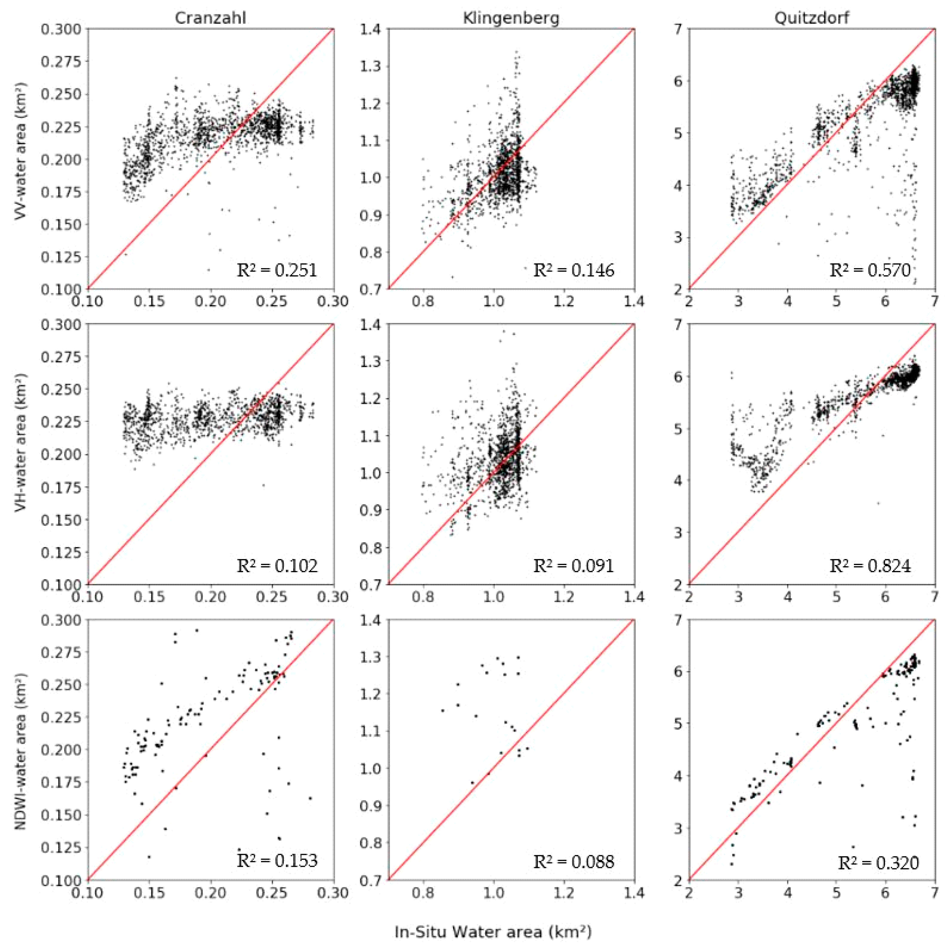
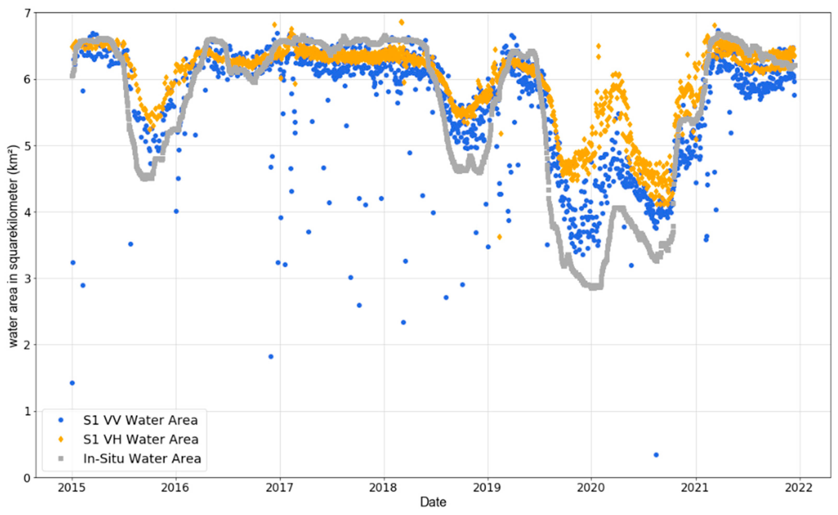
3.2. Validation of the Water Mask Calculation

To validate the WMA results, an analysis was made for the study sites using the vertical–horizontal polarization (VH) and vertical–vertical polarization (VV) bands of the Sentinel-1 and Sentinel-2 index, NDWI. For VV and VH, the first letter describes the polarization direction in which the signal is transmitted from the transmitter. The second letter indicates how the returning signal is received. The calculated water area from each run was compared to in situ data of the surface water extent (Figure 6 and Figure 7). The difference in the number of measurement points between VV/VH and the NDWI is due to the fact that the NDWI is calculated using optical bands. These bands cannot be used when there is cloud cover or night, so, compared to the cloud- and light-independent radar images (VV/VH), there are comparatively few usable images over the selected study period (Figure 6). Radar images from Sentinel-1 allow the evaluation of a much denser time series, which is clearly reflected in the histograms below.
The root-mean-square error (RMSE) and the coefficient of determination (R2), to compare the in situ area data with the WMA area measurements, were calculated for the quality evaluation of the processed data (Table 1). Images with VH polarization show high accuracies with an R2 of 0.824 for Quitzdorf. The prominent indented-shaped Klingenberg reservoir and smaller-sized Cranzahl reservoir only reach low R2-values. In general, it appears that the larger the water body, the higher the RMSE value. When using the NDWI, the highest values are obtained for all AOIs compared to VV and VH RMSEs. The individual comparison between the in situ data and the WMA-calculated area (VV, VH, and the NDWI) for the study areas can be seen in Figure 6.
The water area chart for the Quitzdorf reservoir over a period of seven years (2015–2021) (Figure 7) shows detailed information about the aquatic ecosystem dynamics of the water extent over a seven-year period (2015–2021) (Figure 7). It illustrates that the water level fell during the summer months, especially in the dry years of 2018, 2019, and 2020, due to the absence of precipitation and high evaporation. In addition, the water level in the reservoir was forcibly lowered in 2019 for inspections, which can also be observed. The VV and VH area’s over- and underestimations in Figure 7 for Quitzdorf are clearly visible in the corresponding scatterplots in Figure 6, too.

4. Discussion

As a general pattern for the Sentinel-1 data, the course of the water area calculated by the WMA faces some problems where statistical key figures are affected by outliers. However, there is an overestimation, especially for low water levels, which is most significant in the case of the Sentinel-1 VH data. When the water retrieves quickly, the soil is still wet and can mistakenly be identified as covered with water. Recent studies show that the C-Band-SAR is sensitive to the topsoil layer moisture level [20] but is limited by vegetation cover [21]. Thus, at this point, it is possible that the backscatter of soil moisture is misidentified as a water surface. When a watercourse reaches its full extent, the area tends to be underestimated due to overlapping vegetation and may be favored by other edge effects of pixel-based classification. The measurement error due to vegetation at the watercourse edge increases the smaller such a watercourse is since the proportion of the edge pixels increases in comparison to the surface area of the watercourse. The smaller and more indented-shaped the water areas are, the relatively larger the proportion of the edge pixels is to the total area. This causes several problems in water mask extraction. In addition, for weakly dynamic water bodies, a low R² says little about the quality of the measurement. Here, the point-inspector can serve as a better tool for analyzing the inner pixels of a water body that are not influenced by edge effects.
For determining maximum surface water extents, e.g., the analysis of flood events, Sentinel-1 VH-polarized radar images are more usable due to a better contrast ratio along with a lower noise tendency. The higher sensitivity to volume scattering, due to a wider range of detectable backscattering signals over vegetated land surfaces, compared to co-polarized data, proves to be a disadvantage. This can cause an overlapping with the low-backscattering water areas and consequent misclassification of land, leading to the overestimation of the water areas [22,23,24]. Sentinel-1 VV radar data are more sensitive to surface scattering than that of the VH-polarized so that even ripples or small waves have a negative effect due to interfering signals. It leads to noisier images, especially when masking the larger and more wind-exposed water bodies. The consequences are numerous small holes within the derived water layer or heavily distorted thresholds for the classification processing, leading to a significant underestimation of the water area size. The higher sensitivity of VV imagery, especially to wind, results in a higher variance of the data and much more outliers compared to the VH data, which can be clearly seen in Figure 7. A dense time series can help at this point to filter out noisy images due to external factors such as wind and interpolate data gaps.
It can be seen that the WMA reacts very sensitively to changes in the water surfaces, even if the same intensity of decreasing and increasing trends is not achieved for Quitzdorf, as is shown by the in situ data (Figure 7). As soon as such changes become visible, decision-makers can take action, although ultimately, the accurate mapping of the intensity still has its limits.
By separating the outliers and developing correction factors for frequently studied water bodies, an improvement in the accuracies can be expected in the future for all investigated calculations (VV, VH, and the NDWI water area).
It is also noteworthy that the final water mask, due to the summation of overlapping pixels of the different orbits, reveals details at a spatial resolution in the subpixel range.
The Otsu method [17] itself also reaches its limit and should be critically reviewed or even replaced by other methods in the future. The histogram, on the basis of which the threshold value is formed, is strongly dependent on the placement of the examination AOI and the number of water pixels it contains so that the threshold value varies from image to image. Although the method has already named advantages, a threshold value “correct” for a long time series should not subject each image to changes and thus affect the classification. The temporal resolution is limited by the chosen satellite system. The WMA itself is recommended and optimized for use with Sentinel-1 datasets. The use of optical data (Sentinel-2 and Landsat 8) is mainly intended as Supplementary Information. Using this chosen system, in particular, is expected to result in the availability of an increasingly longer time series in the future. The WMA is designed for the use of free data, which is why users of commercial data experience a limitation here. Fast mapping, as in the case of floods, is only possible if the satellite has an overflight at the right time. Long-term dynamics and trends, on the other hand, can be mapped with the WMA in any case.
A longer time series also means a longer processing time, so users with unrealistic expectations of waiting time for product delivery may be discouraged.
Due to the spatial pixel resolution of the satellite imagery used, small ponds (>0.005 km2) and narrow rivers (>50 m wide) cannot be imaged with the WMA.

5. Conclusions

Even in the current state of development, the WMA offers a fast, always web-based, accessible, and user-friendly service for determining the area and dynamics of water bodies of interest, supported by a well-researched classification method and allows the application even with little previous knowledge. Individual questions of the WMA user are supported here by the use of a variety of setting options and tools.
Small and unfavorably shaped water bodies face major challenges in measuring water area and dynamics. The original water area calculation of the WMA does not achieve the desired results here, but it can be replaced by using the point inspector, which is also offered. The larger a water body is, the more the edge effects fade into the background, with good results in VV polarization.
There is still a need for the development of the WMA based on technical limitations, new technical possibilities, and legal restrictions. In general, varieties of methods are available to delineate land from water. Up to now, the WMA has been working mainly with the proven method of delimitation based on limit values, according to Otsu [17]. However, with today’s possibilities in data processing, new routines in machine and deep learning are available, and these have not yet been tested in the context of the WMA. By using these methods, the entire procedure could be made more efficient, and the results of the water–land delineation could be further improved. As classifiers, support vector machines (SVM), random forests (RFs), and neural networks are the main focus of further development. These have also proven their worth related to land cover classification, as numerous studies have shown [15,16]. In addition, there is potential in the use of external data sets [25] to train deep learning algorithms.
In the further course of development, Germany-wide data sets will be available and significantly increase the pool of in situ data and the range of dynamic water body types. This in situ data will provide a much better indication of the methods’ performance than, for example, specially selected scenes and indices for comparison [13]. The developer is not tempted to select only well-fitting scenes for comparison in order to be able to propagate the highest possible accuracy.
The previous method uses data from only one sensor system, e.g., Sentinel-1. The issue of data fusion has not yet been addressed. Here, advantages for the quality of the water–land boundary dynamics can possibly be derived. Various studies [26] prove that combining SAR and optical data improves the accuracy of classification results compared to separate specific data sets. Especially for standing waters, the addition of elevation models can also counteract possible sources of error in the classification algorithms.

Supplementary Materials

The GEE code is online and freely available at https://code.earthengine.google.com/74692b50b1eb7cdd4bda9a26c4e02b8c?runCode=true&hideCode=true (short-URL: https://bit.ly/3wEdnMI; Google account required).

Author Contributions

Conceptualization, S.B. and S.G.; methodology, S.B.; software, S.B. and M.L.; validation, S.G.; formal analysis, S.B. and S.G.; investigation, S.B.; data curation, S.G.; writing—original draft preparation, S.B., M.L. and S.G.; writing—review and editing, S.G.; visualization, S.B. and S.G.; supervision, S.G.; project administration, S.G.; funding acquisition, S.G. All authors have read and agreed to the published version of the manuscript.

Funding

This research received no external funding.

Acknowledgments

We are grateful that Google Earth Engine provides computational capacities and Sentinel data free of charge.

Conflicts of Interest

The authors declare no conflict of interest. The funders had no role in the design of the study, in the collection, analysis, or interpretation of the data, in the writing of the manuscript, or in the decision to publish the results.

References

  1. Xing, L.; Tang, S.; Wang, H.; Fan, W.; Wang, G. Monitoring monthly surface water dynamics of Dongting Lake using Sentinel-1 data at 10 m. PeerJ 2018, 6, e4992. [Google Scholar] [CrossRef] [PubMed]
  2. Busker, T.; de Roo, A.; Gelati, E.; Schwatke, C.; Adamovic, M.; Bisselink, B.; Pekel, J.-F.; Cottam, A. A global lake and reservoir volume analysis using a surface water dataset and satellite altimetry. Hydrol. Earth Syst. Sci. 2019, 23, 669–690. [Google Scholar] [CrossRef]
  3. Quang, D.N.; Linh, N.K.; Tam, H.S.; Viet, N.T. Remote sensing applications for reservoir water level monitoring, sustainable water surface management, and environmental risks in Quang Nam province, Vietnam. J. Water Clim. Chang. 2021, 12, 3045–3063. [Google Scholar] [CrossRef]
  4. Lefebvre, G.; Davranche, A.; Willm, L.; Campagna, J.; Redmond, L.; Merle, C.; Guelmami, A.; Poulin, B. Introducing WIW for Detecting the Presence of Water in Wetlands with Landsat and Sentinel Satellites. Remote Sens. 2019, 11, 2210. [Google Scholar] [CrossRef]
  5. Förderrichtlinie Teichwirtschaft und Naturschutz (Funding Guideline Pond Management and Nature Conservation). Available online: https://www.revosax.sachsen.de/vorschrift/16010-Foerderrichtlinie-Teichwirtschaft-und-Naturschutz (accessed on 3 May 2022).
  6. Pekel, J.-F.; Cottam, A.; Gorelick, N.; Belward, A.S. High-resolution mapping of global surface water and its long-term changes. Nature 2016, 540, 418–422. [Google Scholar] [CrossRef]
  7. Global Surface Water Explorer. Available online: https://global-surface-water.appsport.com (accessed on 10 January 2022).
  8. Muro, J.; Canty, M.; Conradsen, K.; Hüttich, C.; Nielsen, A.A.; Skriver, H.; Remy, F.; Strauch, A.; Thonfeld, F.; Menz, G. Short-Term Change Detection in Wetlands Using Sentinel-1 Time Series. Remote Sens. 2016, 8, 795. [Google Scholar] [CrossRef]
  9. Li, Y.; Niu, Z.; Xu, Z.; Yan, X. Construction of High Spatial-Temporal Water Body Dataset in China Based on Sentinel-1 Archives and GEE. Remote Sens. 2020, 12, 2413. [Google Scholar] [CrossRef]
  10. Jiang, Z.; Jiang, W.; Ling, Z.; Wang, X.; Peng, K.; Wang, C. Surface Water Extraction and Dynamic Analysis of Baiyangdian Lake Based on the Google Earth Engine Platform Using Sentinel-1 for Reporting SDG 6.6.1 Indicators. Water 2021, 13, 138. [Google Scholar] [CrossRef]
  11. Markert, K.N.; Markert, A.M.; Mayer, T.; Nauman, C.; Haag, A.; Poortinga, A.; Bhandari, B.; Thwal, N.S.; Kunlamai, T.; Chishtie, F.; et al. Comparing Sentinel-1 Surface Water Mapping Algorithms and Radiometric Terrain Correction Processing in Southeast Asia Utilizing Google Earth Engine. Remote Sens. 2020, 12, 2469. [Google Scholar] [CrossRef]
  12. Gorelick, N.; Hancher, M.; Dixon, M.; Ilyushchenko, S.; Thau, D.; Moore, R. Google Earth Engine: Planetary-scale geospatial analysis for everyone. Remote Sens. Environ. 2017, 202, 18–27. [Google Scholar] [CrossRef]
  13. Soman, M.K.; Indu, J. Sentinel-1 basied inland water dynamics Mapping System (SIMS). Env. Model. Software 2022, 149, 105305. [Google Scholar] [CrossRef]
  14. Landestalsperrenverwaltung Sachsen (State Dams Administration Saxony). Talsperrenmeldezentrale. Available online: https://www.ltv.sachsen.de/tmz/uebersicht.html (accessed on 2 May 2022).
  15. Mira, N.C.; Catalao, J.; Nico, G. Multi-temporal crop classification with machine learning techniques. Remote Sens. Agric. Ecosyst. Hydrol. XXI 2019, 111490P. [Google Scholar] [CrossRef]
  16. Phan, T.N.; Kuch, V.; Lehnert, L.W. Land Cover Classification using Google Earth Engine and Random Forest Classifier—The Role of Image Composition. Remote Sens. 2020, 12, 2411. [Google Scholar] [CrossRef]
  17. Otsu, N. A threshold selection method from gray-level-histograms. IEEE Trabs. Syst. Man. Cybern. 1979, 9, 62–66. [Google Scholar] [CrossRef]
  18. Li, J.; Wang, S. An automatic method for mapping inland surface waterbodies with Radarsat-2 imagery. Int. J. Remote Sens. 2015, 36, 1367–1384. [Google Scholar] [CrossRef]
  19. Lee, J.; Jurkevich, L.; Dewaele, P.; Wambacq, P.; Oosterlinck, A. Speckle filtering of synthetic aperture radar images: A Review. Remote Sens. Rev. 1994, 8, 313–340. [Google Scholar] [CrossRef]
  20. Macelloni, G.; Paloscia, S.; Pampaloni, P.; Sigismondi, S.; De Matthaeis, P.; Ferrazzoli, P.; Schiavon, G.; Solimini, D. The SIR-C/X-SAR experiment on Montespertoli: Sensitivity to hydrological parameters. Int. J. Remote Sens. 1999, 20, 2597–2612. [Google Scholar] [CrossRef]
  21. Shi, J.; Chen, K.S.; Li, Q.; Jackson, T.J.; O’Neill, P.E.; Tsang, L. A parameterized surface reflectivity model and estimation of bare-surface soil moisture with L-band radiometer. IEEE Trans. Geosci. Remote Sens. 2002, 40, 2674–2686. [Google Scholar]
  22. Manjusree, R.; Kumar, L.P.; Bhatt, C.M.; Rao, G.S.; Bhanumurthy, V. Optimization of threshold ranges for rapid flood inundation mapping by evaluating backscatter profiles of high incidence angle SAR images. Int. J. Disaster Risk Sci. 2012, 3, 113–122. [Google Scholar] [CrossRef]
  23. Twele, A.; Cao, W.X.; Plank, S.; Martinis, S. Sentinel-1-based flood mapping: A fully automated processing chain. Int. J. Remote Sens. 2016, 37, 2990–3004. [Google Scholar] [CrossRef]
  24. Clement, M.; Kilsby, C.; Moore, P. Multi-temporal synthetic aperture radar flood mapping using change detection. J. Flood Risk Manag. 2017, 11, S152–S168. [Google Scholar] [CrossRef] [Green Version]
  25. Bonafilia, D.; Tellman, B.; Anderson, T.; Issenberg, E. Sen1Floods11: A georeferenced dataset to train and test deep learning flood algorithms for Sentinel-1. In Proceedings of the 2020 IEEE/CVF Conference on Computer Vision and Pattern Recognition Workshops (CVPRW), Seattle, WA, USA, 14–19 June 2020; pp. 835–845. [Google Scholar] [CrossRef]
  26. Joshi, N.; Baumann, M.; Ehammer, A.; Fensholt, R.; Grogan, K.; Hostert, P.; Jepsen, M.R.; Kuemmerle, T.; Meyfroidt, P.; Mitchard, E.T.A.; et al. A Review of the Application of Optical and Radar Remote Sensing Data Fusion to Land Use Mapping and Monitoring. Remote Sens. 2016, 8, 70. [Google Scholar] [CrossRef] [Green Version]
Figure 1. Use of Otsu’s method for a defined (a) AOI of the Quitzdorf reservoir that shows the (b) characteristic water–land pixel value distribution in the corresponding histogram of an exemplary Sentinel-1 median radar image with VV-polarization.
Remotesensing 14 04485 g001
Figure 2. The locations and shapes of three investigated water bodies in Saxony, Germany. Projection and coordinate system: ETRS89/UTM32N, EPSG: 25832.
Remotesensing 14 04485 g002
Figure 3. Pre-processing map view.
Remotesensing 14 04485 g003
Figure 4. Processing scheme of WMA.
Remotesensing 14 04485 g004
Figure 5. Post-processing map view of WMA.
Remotesensing 14 04485 g005
Figure 6. WMA-measured water area (km2) in VV and VH polarization and by the NDWI compared to the in situ water area (km2) for the period from 1 January 2016 to 31 December 2021. The red line marks the coincidence between the measured value and the in situ value.
Remotesensing 14 04485 g006
Figure 7. Time series for the water area in VV and VH polarization and in situ data for the Quitzdorf reservoir. Time period from 1 January 2015 to 31 December 2021.
Remotesensing 14 04485 g007
Table 1. Quality parameters of the WMA water area measurements from 1 January 2016 until 31 December 2021 in relation to the in situ data.
Sensor/IndexParameterCranzahlKlingenbergQuitzdorf
Sentinel-1 VVR20.2510.1460.570
RMSE (km2)0.0400.0770.863
Sentinel-1 VHR20.1020.0910.824
RMSE (km2)0.0480.0850.708
Sentinel-2 NDWIR20.1530.0880.320
RSME (km2)0.0650.3231.276
Publisher’s Note: MDPI stays neutral with regard to jurisdictional claims in published maps and institutional affiliations.

