Abstract
Three dimensional (3D) green volume is an important tree factor used in forest surveys as a prerequisite for estimating aboveground biomass (AGB). In this study, we developed a method for accurately calculating the 3D green volume of single trees from unmanned aerial vehicle laser scanner (ULS) data, using a voxel coupling convex hull by slices algorithm, and compared the results using voxel coupling convex hull by slices algorithm with traditional 3D green volume algorithms (3D convex hull, 3D concave hull (alpha shape), convex hull by slices, voxel and voxel coupling convex hull by slices algorithms) to estimate AGB. Our results showed the following: (1) The voxel coupling convex hull by slices algorithm can accurately estimate the 3D green volume of a single ginkgo tree (RMSE = 11.17 m3); (2) Point cloud density can significantly affect the extraction of 3D green volume; (3) The addition of the 3D green volume parameter can significantly improve the accuracy of the model to estimate AGB, where the highest accuracy was obtained by the voxel coupling convex hull by slices algorithm (CV-R2 = 0.85, RMSE = 11.29 kg, and nRMSE = 15.12%). These results indicate that the voxel coupling convex hull by slices algorithms can more effectively calculate the 3D green volume of a single tree from ULS data. Moreover, our study provides a comprehensive evaluation of the use of ULS 3D green volume for AGB estimation and could significantly improve the estimation accuracy of AGB.
1. Introduction
The three-dimensional (3D) green volume of an urban forest could be defined as the volume of space occupied by all green stems and leaves of plants in the city [1,2,3,4,5], which reflects the ecological functions and environmental benefits of urban forests in terms of spatial patterns. Thus, it has been well established that 3D green volume plays important roles in the estimation of aboveground biomass (AGB), the estimation of the environmental benefits of greening, and the construction of forest fire risk models, thus, effectively improving the efficiency of urban green space evaluation and green space planning [6,7,8,9]. However, urban forests are composed of scattered trees, tree belts, forests with structural diversity, and forests with broken distribution [10]. They are very different from the large, continuously distributed forests in the general sense, thus, making the monitoring and evaluation of urban forest resources complicated. How to accurately estimate the 3D green volume and AGB of urban forests has become an urgent problem to be solved.
Methods for measuring 3D green volume currently include field measurements, optical remote sensing estimation, and LiDAR estimation. The most widely used manual method for estimating canopy volume is the ellipsoidal method, in which crown diameters and canopy heights are measured, assuming an ellipsoidal shape for the canopy [9]. The disadvantage of this method is the large workload, and low efficiency, and it is difficult to carry out a wide range of extensions. Optical remote sensing estimation is mainly based on single-tree crown diameter extraction from high-resolution images combined with ground measured data and on building crown diameter–crown height models to perform 3D green volume estimation. This method has achieved good results in related research in China [11], but it is difficult to comprehensively obtain the vertical distribution of forest structure. The accuracy of the model needs to be further improved [12]. Light detection and ranging (LiDAR) are an active remote sensing technique using pulsed or continuous-wave lasers to measure the range of an object that can rapidly obtain dense 3D point clouds with high precision. Moreover, LiDAR has become a trending topic of domestic and international research because it can describe the forest canopy structure in more detail and provide advanced technical means for accurate estimation of 3D green volume by enabling the leap from two-dimensional (2D) to 3D forest ecosystem research [13,14,15,16,17].
A review of domestic and foreign literature found that the main algorithms for 3D green volume estimation, based on LiDAR point clouds, include 3D convex hulls, 3D concave hulls (alpha shape), convex hulls by slices, and voxels. For example, Ebadat et al. [18] used unmanned aerial vehicle laser scanner (ULS) and photogrammetric point cloud to extract 3D green volume based on a 3D convex hull algorithm. The results showed that UAV photogrammetry and LiDAR point clouds were highly correlated (R2 = 0.99). Vauhkonen et al. [19] extracted canopy volume based on ALS data. using the alpha shape algorithm, and used it to estimate wood volume. He et al. [2] calculated the 3D green volume based on terrestrial laser scanner (TLS) data. using the convex hull by slices algorithm. and better obtained the 3D green volume of the Beijing urban forest (R2 > 0.85). Fernández-Sarría et al. [20] extracted the 3D green volume of overhanging trees, using a voxel algorithm, based on TLS data (R2 = 0.78), and the results showed that TLS has some potential in predicting the 3D green volume of urban forests. How to choose the appropriate algorithm and input parameters is the current problem faced by researchers.
LiDAR can accurately extract structural parameters, such as crown projection area, crown diameter, and crown height, which makes it advantageous for single-tree AGB estimation [21,22,23]. Three dimensional green volume characterizes the volume of space occupied by plants. Therefore, the participation of 3D green volume in the estimation of AGB has attracted extensive attention from scholars. For example, Tao et al. [24] showed that a 3D green biomass incorporation model could more accurately estimate the AGB (R2 = 0.77, RMSE = 179.0 Mg/ha). Hauglin et al. [6] estimated the AGB of a single tree plant based on TLS extraction of voxelization parameters with higher accuracy than conventional anisotropic growth models (R2 = 0.88, RMSE% = 32%).
LiDAR data acquisition includes TLS, airborne laser scanner (ALS), and ULS. The laser radar scanner installed on the TLS ground support obtains a high-density point cloud, but it takes a great deal of time to collect TLS data. due to its static properties, so its use cannot be widely promoted [25]. ALS can obtain a wide range of 3D point cloud data, but low point cloud density makes it impossible to accurately express stand structure [9]. Conversely, ULS can efficiently acquire large-area point cloud data, and compared with ALS, ULS flies at lower altitudes and can acquire a higher point cloud density [26]. However, there are few studies on the extraction of single tree 3D green volume based on ULS [18].
Ginkgo (Ginkgo biloba L.) is widely distributed in China and East Asia, with the advantages of an upright trunk, beautiful tree shape and strong resistance to diseases, etc. It is an important tree species for urban greening and has high economic and ecological value. It is of great significance to obtain accurate structural parameters of single Ginkgo trees. This study developed a new algorithm to calculate tree 3D green volume from ULS data. Coupled voxel and convex hull by slices algorithms provide a more accurate calculation of 3D green volume, compared with those achieved using conventional algorithms. The objectives of this study were the following: (1) to select the optimal algorithm for single tree 3D green volume extraction based on ULS data, (2) to evaluate the effect of point cloud density variation on 3D green volume, and (3) to compare different 3D green volume algorithms for AGB estimation.
2. Materials and Methods
2.1. Study Area and Data Acquisition
The study area, Zhejiang A&F University (Figure 1), is situated in Lin’an, Hangzhou, Zhejiang Province. The geographical coordinates of Lin’an city are 30°15′10″~30°15′30″N, 119°43′10″~119°43′40″E. The area is dominated by hilly and mountainous terrain, and the terrain slopes from west to southeast. The area has a subtropical monsoon climate, with abundant light and abundant rainfall. The average annual precipitation is 1613.9 mm, with 158 days of precipitation, and the average annual frost-free period is 237 days. The average elevation of the study area is approximately 50 m, and the area is covered with ginkgo trees on both sides of Ginkgo avenue.
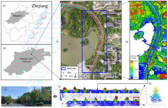
Figure 1.
Overview of the study area. (a) location of Hangzhou, (b) location of the study area, (c) aerial photograph of the study area, (d) ULS point cloud of the study area, (e) ground image of ginkgo, (f) ULS point cloud of ginkgo, (g) point cloud of a single tree of ginkgo.
Field work was conducted in July 2021. Data from 64 single ginkgo trees were measured. The coordinates of each single tree were located using a real-time kinematic (RTK) device. The diameter at breast height (DBH) was measured using a diameter tape. The single-tree height and branch height were measured using a hypsometer, and the north–south and east–west crown diameters were measured using a tape rule [27]. Crown height is tree height minus branch height [28]. The crown diameter is the average of the east–west and north–south crown diameters. The single-tree 3D green volume values were calculated according to the crown diameter and crown height based on the volume of the geometry [9]. The single-tree AGB values were calculated according to the tree height and DBH, based on the biomass allometric model developed by [29]. The measured forest structural attributes for the single trees are summarized in Table 1.

Table 1.
Descriptive statistics of field inventory data for 64 trees.
2.2. ULS Data
The ULS data for this study were acquired in May 2021. The DJI Matrice 600 Pro six-rotor unmanned aerial vehicle (UAV) was used in clear-weather and low-wind conditions. Using the Velodyne Puck LITETM sensor to obtain the original ULS point cloud, the sensor records the first echo of the pulse, with a flight altitude of 60 m, flight speed of 5 m/s, swath width of 25 m, and route overlap rate of 50%, with an average point cloud density of approximately 230 pts.
2.3. ULS Metrics
The ULS point cloud was preprocessed using LiDAR360 software. First, the single-tree point cloud was denoised and filtered. Then, classification of ground points was carried out using the improved progressive TIN densification (IPTD) algorithm [30] and a digital elevation model (DEM), with a resolution of 0.5 m generated by irregular triangulation interpolation [31]. Finally, the point cloud data were normalized to remove topographic fluctuations from the data. Point clouds above 2 m were extracted as canopy point clouds, and three sets of metrics were computed (Table 2) [32,33].
Table 2.
Description of metrics derived from ULS data.
2.4. Green Volume Calculation Algorithm
2.4.1. Convex Hull Algorithm
A convex hull is a concept in computational geometry defined as finding a minimal set of points such that the shape formed by the set of points can contain all points in the 2D plane or 3D space [34]. Figure 2a shows a schematic diagram of the 2D convex hull. In this study, the point cloud of a single tree canopy is projected to the 2D plane, the 2D convex hull is calculated, and the projected area of the canopy is extracted based on the convhull function in MATLAB. Figure 2b shows the results of the convex hull algorithm in 3D space, based on the quickhull algorithm to reconstruct the canopy surface and calculate the volume under the convex hull, i.e., the 3D green volume [20].
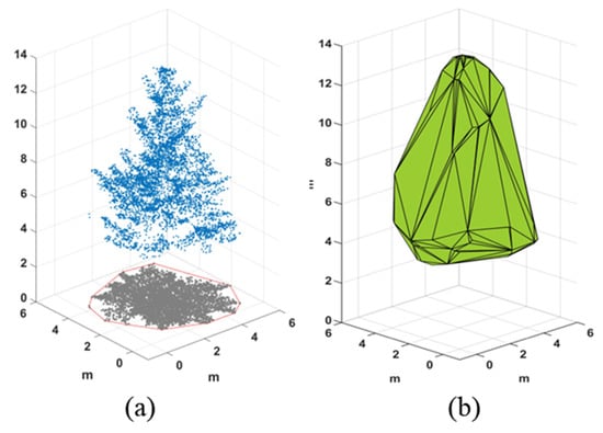
Figure 2.
(a) A schematic diagram of a 2D convex hull algorithm, and (b) An example of a 3D convex hull algorithm.
2.4.2. Concave Hull Algorithm
The concave hull algorithm is another common geometric calculation method, which can be understood as an additional parameter alpha that can be set on top of the convex hull, with alpha as the diameter of the circle rolling along the boundary of the convex polyhedron. The trajectory of the rolling circle is the boundary of the concave polyhedron [19], so the method is also called alpha shape. The algorithm is shown in Figure 3a. The process of reconstructing the shape of the tree crown in the 3D concave hull does not connect vertices that are too far apart, as in the 3D convex hull. If alpha tends to infinity, the concave hull result is infinitely close to the convex hull, while a smaller alpha tends to be concave at a certain position to fit the shape of the point set more closely [35,36]. The results of the concave packet algorithm with different parameters on a tree are shown in Figure 3b. In this study, we set the alpha range as 0.1–5 m, took 0.1 m as a step and calculated the RMSE with measured 3D green volume to select the optimal scale.
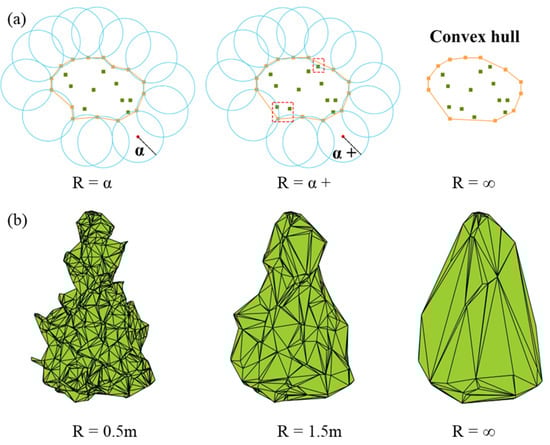
Figure 3.
(a) The schematic diagram of the concave hull algorithm (b) The single tree contour constructed by the concave hull with different parameters.
2.4.3. Convex Hull by Slices Algorithm
The convex hull by slices algorithm is based on the idea of integration. First, the canopy is sliced according to the uniform thickness, and each layer is considered a table body. For each layer, the point clouds within 0.2 m of each plane are counted, these point clouds are projected to the same plane, and the projected area of the plane is calculated using the 2D convex hull algorithm. Then, the table product formula is used to calculate the volume of each layer. Finally, all the slice volumes are summed to obtain the 3D green volume (Figure 4) [27,37]. The convex hull by slices algorithm sets the height difference in the range of 0.1–5 m with a step of 0.1 m, and calculates the RMSE with measured 3D green volume to select the optimal scale. The volume of each layer of the table is calculated as follows:
where is the projected area of the nth layer of the point cloud calculated based on the 2D convex packet algorithm and is the height of the table.
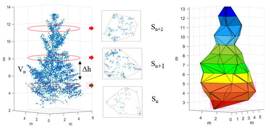
Figure 4.
The schematic diagram of the convex hull by slices algorithm.
2.4.4. Voxel Algorithm
The voxel algorithm uses a regular 3D grid to partition the discrete canopy point cloud. The initialized grid is divided into N smaller voxels according to the input parameters, and the number of voxels in which at least one point exists in the statistical space is determined, based on the range of the canopy point cloud to determine the polar values of the starting grid in the XYZ coordinate directions. The sum of the space volumes occupied by the voxels is the 3D green volume (Figure 5) [28,38]. In this study, the voxel edge length was set in the range of 0.1–1 m, the step length was 0.1 m, and the RMSE was calculated with measured 3D green volume to select the optimal scale.
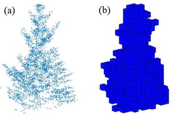
Figure 5.
(a) The single tree point clouds (b) The schematic diagram of the voxel algorithm.
2.4.5. Voxel Coupling Convex Hull by Slices Algorithm
The 3D convex hull algorithm treats the canopy as a whole and cannot calculate the gaps within the canopy, and its boundary does not represent the real canopy outline, and, thus, it overestimates the measured 3D green volume [1,8]. The concave hull algorithm excessively removes voids and gaps when calculating the volume, leading to low 3D green volume estimation results [39]. Since the crown shape and size of different single trees of the same species vary greatly, uniform thickness slices in the vertical direction bring some errors to the calculation of 3D green volume based on the convex hull by slices algorithm [40]. The voxel algorithm can generate realistic canopy shapes to obtain high-accuracy 3D green volume [28,41], but the missing ULS point cloud leads to underestimation of 3D green volume [9]. Figure 6 shows a single tree ginkgo canopy for the voxel algorithm, and it can be seen that the point cloud absence increases with decreasing height.
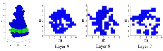
Figure 6.
Single tree voxel profile analysis (Layer 7, Layer 8, Layer 9 shows the horizontal section of the tree at a crown height of 2.8 m, 3.2 m, and 3.6 m).
Based on the above analysis, a new algorithm for 3D green volume estimation, named voxel coupling convex hull by slices, is proposed in this study. The method calculates the 3D green volume by dividing the single tree canopy point cloud into two parts according to height, and the volume of the upper canopy point cloud is calculated using the voxel algorithm, to prevent the calculation error of the upper layer caused by uniform thickness slicing, while the volume of the lower canopy point cloud is calculated using the convex hull by slices algorithm, to prevent the calculation error of the green volume caused by the missing point cloud of the lower layer (Figure 7). To explore the optimal stratification ratio, this study set the stratification range, from 10% to 90%, with a step size of 10%, extracted the 3D green volume of each stratification, and calculated the RMSE with measured 3D green volume to select the optimal scale. The computational equations of this new method are shown below:
where n is the number of voxels, is the volume of a single voxel, is the projected area of the nth layer of the point cloud, and is the height of the table.
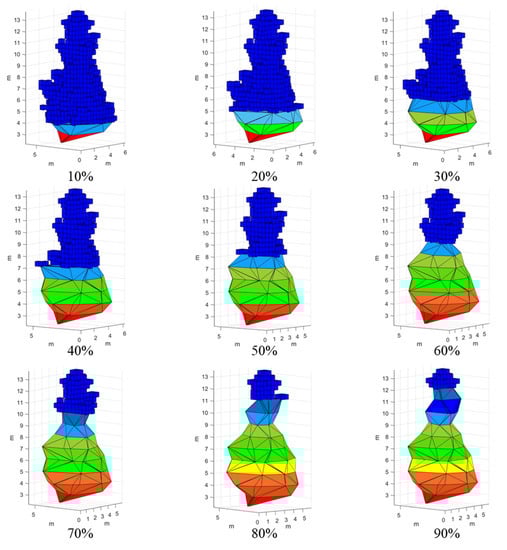
Figure 7.
Schematic diagram of the voxel coupling convex hull by slices algorithm.
2.5. Sensitivity Analysis of ULS Data Density
To explore the effect of different LiDAR point cloud densities on extracting 3D green volume, the original point density (230 pts/m2) was used to lower densities to 75% (172.5 pts/m2), 50% (115 pts/m2), 25% (57.5 pts/m2), 10% (23 pts/m2) and 5% (11.5 pts/m2). We used a point cloud height-based algorithm that groups all point clouds by elevation and extracts reduced point clouds by percentage in each layer [15,42]. This algorithm ensured the consistency of sampling, and the extracted point cloud data could maintain a similar spatial distribution as the original point cloud data.
2.6. Random Forest Model
The RF algorithm, created by Breiman and Cutler, was developed as an integrated learning model and a basic decision tree classifier. The decision tree algorithm is an extension of the conventional framework. It improves prediction accuracy by combining multiple decision trees [43,44]. The basic idea is that by using bootstrapping with repeated sampling replacement from several random samples, and establishing a corresponding decision tree for each sample, a RF could be constituted by combining the forecasting of multiple decision trees [45].
The randomForest function under the randomForest data package in R software was used to construct the RF model. First, in the method using the random forest R language, the program determines the influence of each independent variable on the regression process and then evaluates the influence using two indexes. One is the model mean square error (%InMSE) increment when out-of-bag arguments appear, and the second is the impact of purity on the tree node model when out-of-bag arguments arise. Second, the RF algorithm has three important parameters: ntree is the number of random regression trees; nodesize is the minimum size of the terminal node, whose default value is 5; and mtry is a variable division number (the default value is one-third of the number of arguments). In this study, ntree was set to 2000, and the rest of the parameters were set as default parameters. The effect of each independent variable was determined based on the out-of-bag error (%InMSE) [43] (Figure 8).
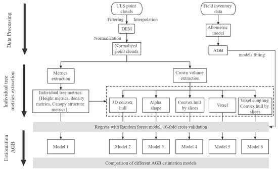
Figure 8.
The flow chart of this study.
2.7. Model Verification
In this study, the R2, RMSE, and nRMSE of 10-fold cross-validation were used to evaluate the model fit. Generally, a higher accuracy is indicated by higher values of R2 and lower values of RMSE and nRMSE. R2, RMSE and nRMSE were calculated as follows:
where represents the observed AGB for the ith tree, is the observed mean value, is the estimated AGB for the ith tree, and n is the number of trees.
3. Results
3.1. Determination of Different 3D Green Volume Algorithm Parameters
Figure 9 shows that in the alpha shape algorithm, as the alpha parameter increased, the 3D green volume also became larger, and the alpha value tended to stabilize after 2 m. The RMSE showed first a decreasing and then an increasing trend, with a peak at the 0.6 m scale, and tended to stabilize after the alpha value was greater than 1.3 m. The RMSE under this scale was 12.20 m3. The overall trend of the 3D green volume obtained by the convex hull by slices algorithm decreased with increasing height interval, and the RMSE did not change regularly, but, overall, the RMSE was higher when the height interval was higher, with a peak at the 0.9 m scale. The RMSE under this scale was 13.01 m3. The 3D green volume obtained by the voxel algorithm increased linearly with increasing voxel size, and the RMSE showed a trend of first decreasing and then increasing, peaking at a scale of 0.4 m. The optimal voxel size was selected as 0.4 × 0.4 × 0.4 m, and the RMSE at this scale was 12.03 m3. Figure 10 shows the results of the voxel coupling convex hull by slices algorithm. As the segmentation scale increased, the RMSE decreased and then increased. The optimal canopy segmentation scale was selected to be 20%, and the RMSE at this scale was 11.17 m3, which was lower than those of the other algorithms.
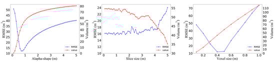
Figure 9.
Optimization of different algorithm parameters.
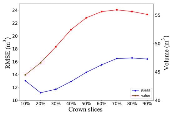
Figure 10.
Stratified scale screening.
3.2. Calculation Results of 3D Green Volume
The 3D green volume of single ginkgo trees differed significantly, due to differences in growth. The results of the 3D green volume calculated using the five algorithms, 3D convex hull, 3D concave hull, convex hull by slices, voxel and voxel coupling convex hull by slices, are shown in Table 3. The average 3D green volume and RMSE calculated by the 3D convex hull algorithm was much higher than those calculated by the other models, ranging from 21.22–196.10 m3 (mean = 84.86 m3, RMSE = 45.31 m3). The average 3D green volume calculated by the 3D concave hull was the lowest, ranging from 12.12–74.84 m3 (mean = 37.72 m3, RMSE = 12.20 m3). The convex hull by slices algorithm overestimated 3D green volume, and ranged from 15.16–133.53 m3 (mean = 53.85 m3, RMSE = 13.01 m3), and the 3D green volume calculated by the voxel algorithm ranged from 16.00–81.79 m3 (mean = 43.13 m3, RMSE = 12.03 m3). The average 3D green volume calculated by the voxel coupling convex hull by slices algorithm ranged from 15.58–97.20 m3 (mean = 46.61 m3), and the 3D green volume calculated by this method was the minimum RMSE (11.17 m3).
Table 3.
Three dimensional green volume of single trees of ginkgo by different algorithms.
3.3. ULS Point Density Effects on the Performance of the 3D Green Volume
To investigate the effects of ULS point density on 3D green volume, we calculated using 5 algorithms with different sampling densities of 75% (172.5 pts/m2), 50% (115 pts/m2), 25% (57.5 pts/m2), 10% (23 pts/m2) and 5% (11.5 pts/m2) and the Pearson’s correlation between AGB and 3D green volume (Figure 11). The box plot in Figure 11 shows the changes in the 3D green volume values due to the decrease in point cloud density. The 3D green volume values and r values of all five algorithms decreased as the point cloud density decreased; among them, the values of the 3D convex hull and convex hull by slices algorithm decreased slowly with the point cloud density from 100% (230 pts/m2) to 10% (23 pts/m2), and the correlation with the AGB was stable. However, when the point density decreased to 5% (11.5 pts/m2), there was a marked decrease in the r values and 3D green volume values (3D convex hull, r = 0.88–0.86; convex hull by slices, r = 0.84–0.80). For the alpha shape and voxel algorithms, there was a slight downward trend in the 3D green volume value and r values as the point cloud density decreased from 100% (230 pts/m2) to 50% (115 pts/m2), and as the point cloud density decreased from 50% (115 pts/m2) to 5% (11.5 pts/m2), the metric and r values decreased significantly (alpha shape, r = 0.84–0.70; voxel r = 0.87–0.80). The 3D green volume values of voxel coupling convex hull by slices algorithm decreased with point cloud density in the same way as the voxel algorithm, but the decrease in r values was lower (0.87–0.84). Therefore, this study chose to extract single-tree 3D green volume at 100% (230 pts/m2) of point cloud density as a metric to estimate AGB.
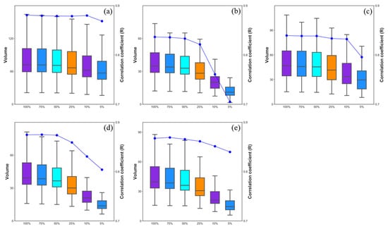
Figure 11.
Distribution and correlation with AGB of 3D convex hull (a), 3D concave hull (b), convex hull by slices (c), voxel (d) and voxel coupling convex hull by slices (e) algorithms at different point densities (100%, 75%, 50%, 25%, 10%, 5%).
3.4. RF Variable Importance Analysis
In this study, the 3D green volume extracted by each of the five algorithms was combined with the ULS base parameters to obtain the importance scores of the input variables by adding the RF model for 100 runs. Figure 12 shows a statistical plot of the importance scores of the top 20 variables with the greatest impact on the estimated AGB. In all models, 3D green volume, H_99, and H_max were the three parameters with the highest importance; the 3D green volume in model 2 had the second highest importance after H_99; the 3D green volume in model 3 had lower importance than H_99 and H_max; and the 3D green volume in models 4, 5 and 6 were the parameters with the highest importance. The mean importance of 3D green volume in model 6 was 35.92, which was significantly higher than that of the other parameters. It indicated that 3D green volume is an important parameter for estimating single tree AGB.
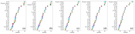
Figure 12.
RF model AGB parameter importance analysis of 3D convex hull (a) 3D concave hull (b) Convex hull by slices (c) Voxel (d) Voxel coupling convex hull by slices (e) % in MSE for the first 20 variables running the RF model 100 times.
3.5. Single-Tree AGB Estimation
The results of different models predicting single tree AGB are shown in Figure 13 and Table 4. The accuracy of model 1, based on ULS base parameters, was CV-R2 = 0.81, RMSE = 12.66 kg, nRMSE = 16.94%, and the AGBs estimated by models 2–5, with the addition of 3D green volume parameters, were better than that of model 1 (CV-R2 = 0.82–0.85, RMSE = 11.29–12.54 kg, nRMSE = 15.12–16.79%). This indicated that the addition of 3D green volume could significantly improve the estimation accuracy of AGB. Model 6 had the highest accuracy (CV-R2 = 0.85, RMSE = 11.29 kg, nRMSE = 15.12%), with an improvement in CV-R2 of 0.04, a decrease in RMSE of 1.37 kg, and a decrease in nRMSE of 1.82%.
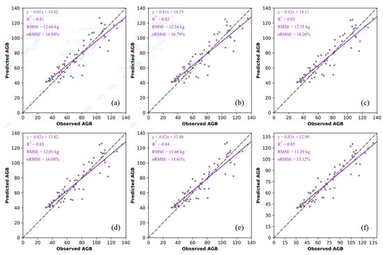
Figure 13.
Different algorithms for estimating AGB (a) ULS basis parameters, (b) 3D convex hull, (c) 3D concave hull, (d) Convex hull by slices, (e) Voxel, (f) Voxel coupling convex hull by slices.
Table 4.
Different algorithms for estimating AGB accuracy.
4. Discussion
Previous studies have shown that lidar pulses are nearly vertical, resulting in the number of point clouds from the lower parts of the crown being lower than those nearer the top, and, thus, ALS tends to underestimate the 3D green volume at the bottom of the canopy [9]. Although the point cloud density obtained by ULS is higher than that of ALS, there is still a problem of missing point clouds inside the bottom layer of the canopy (Figure 6). Alpha shape and voxel algorithms are strongly affected by the point cloud integrity, resulting in an underestimation of 3D green volume [19,46]. Fernández-Sarría et al. [20] found that the 3D convex hull algorithm overestimated the canopy gap, leading to an overestimation of the 3D green volume. Yan et al. [1] argued that the 2D convex hull algorithm would overestimate the projected area of the canopy slices, leading to an overestimation of the 3D green volume by the convex hull by slices algorithm. Our results showed that the 3D concave hull and voxel algorithms underestimated the 3D green volume, and the 3D convex hull and convex hull by slices overestimated the 3D green volume, which was consistent with previous studies. In this study, we described and evaluated a method to estimate the 3D green volume of a single tree and obtained the optimal 3D green volume extraction result (RMSE = 11.17 m3). The voxel coupling convex hull by slices algorithm calculates the 3D green volume at the bottom of the canopy using the convex hull by slices algorithm, which is more stable than the voxel algorithm [1,46] and can solve the underestimation of 3D green volume caused by the missing point cloud at the bottom of the canopy to obtain a more accurate 3D green volume.
Foreign and domestic studies have shown that changes in point cloud density have no significant effect on most ULS metrics [15,39,47]. This study also analyzed the effect of the change in point cloud density on the 3D green volume and found that as the point cloud density decreased from 100% (230 pts/m2) to 75% (172.5 pts/m2), 50% (115 pts/m2), 25% (57.5 pts/m2), 10% (23 pts/m2) and 5% (11.5 pts/m2), the 3D green volume values extracted by all five algorithms and the correlation with AGB decreased as the point cloud density decreased (Figure 11). Our results illustrated that the 3D concave hull algorithm and voxel algorithm were sensitive to the point cloud density; when the point cloud density decreased, the extracted 3D green volume value and correlation decreased considerably. Vauhkonen et al. [44] found that the lower the point cloud density, the lower the accuracy of the concave hull algorithm in predicting single tree features. Liu et al. [29] pointed out that the reduction in point cloud density had a significant effect on the canopy volume metrics extracted based on voxels. The 3D convex hull and convex hull by slices algorithms are more stable because these two algorithms are built based on the convex hull algorithm, which calculates the area (volume) of the entire point set based on the outermost points (planes) and is less affected by changes in point cloud density [1]. The voxel coupling convex hull by slices algorithm is more stable than the voxel algorithm in terms of r value variation, which further indicates that the algorithm solves the effect of missing point clouds in the results of the voxel algorithm.
In this study, 3D green volume was involved in AGB estimation as a parameter, and the analysis of the importance of RF variables showed that 3D green volume was one of the most important parameters for AGB estimation (Figure 11). The accuracy of AGB estimation was significantly improved with the inclusion of the 3D green volume parameter (Figure 12), indicating that 3D green volume had an important influence on AGB estimation, which was consistent with the results of previous studies [24]. The model accuracy showed a significant improvement compared to the AGB accuracy (R2 = 0.77) estimated by [18] based on ALS. This was due to the lower flight altitude of the ULS (60 m) compared with that of the ALS, which enabled a higher density of point cloud data to be acquired, and higher density point cloud data helped to reconstruct the forest 3D structure at a more refined scale [33,48]. Through a comparative analysis, it was found that model 6 predicted AGB with the highest accuracy, because the voxel coupling convex hull by slices algorithm obtained a more accurate 3D green volume, compared to the other algorithms, which made the model fitting ability more accurate.
5. Conclusions
To better extract the 3D green volume of a single tree based on the ULS point cloud, this study proposes the voxel coupling convex hull by slices algorithm, which improves the existing algorithms. To validate the algorithm, the 3D green volume of 64 single ginkgo trees was calculated using this method, and the AGB of single trees was estimated based on the 3D green volume and compared with existing methods. The results showed that the voxel coupling convex hull by slices algorithm was most suitable for calculating the 3D green volume and estimating the AGB using ULS data. The results were as follows: (1) The choice of input parameters of different algorithms significantly affects the results for 3D green volume. Under the premise of using optimal parameters, the voxel coupling convex hull by slices algorithm provided the most accurate estimate of the 3D green volume of single ginkgo trees with RMSE = 11.17 m3; (2). The error in calculating 3D green measures increased for all algorithms as the point cloud density decreased. The concave hull and voxel algorithms had a higher dependence on point cloud density than the other algorithms, and the correlation between AGB and the 3D convex hull, convex hull by slices and voxel coupling convex hull by slices algorithms was more stable when the point cloud density was higher than 10%; (3) The 3D green volume was the most important parameter for estimating the AGB of a single tree. The addition of the 3D green volume parameter could significantly improve the accuracy of the model to estimate AGB, where the highest accuracy was obtained with the voxel coupling convex hull by slices algorithm, which estimated AGB with CV-R2 = 0.85, RMSE = 11.29 kg, and nRMSE = 15.12%. Our study demonstrates that ULS point cloud data can be used to accurately extract the 3D green volume of single trees in urban forests and that the 3D green volume is promising for estimating the AGB of a single tree.
Author Contributions
Conceptualization, H.D. and H.H.; methodology, L.Z.; validation, L.Z.; formal analysis, L.Z.; investigation, L.Z., B.Z., J.X., Y.G. and C.T.; data curation, L.Z.; writing—original draft preparation, L.Z.; writing—review and editing, X.L. and H.D.; visualization, L.Z.; supervision, H.D. All authors have read and agreed to the published version of the manuscript.
Funding
The authors gratefully acknowledge the support of the National Natural Science Foundation of China (U1809208, 32171785, 32201553), the State Key Laboratory of Subtropical Silviculture (No. ZY20180201), and the Key Research and Development Program of Zhejiang Province (2021C02005).
Data Availability Statement
Not applicable.
Acknowledgments
The authors gratefully acknowledge the support of various foundations. The authors are grateful to the editor and anonymous reviewers whose comments have contributed to improving the quality of this manuscript.
Conflicts of Interest
The authors declare no conflict of interest.
References
- Yan, Z.; Liu, R.; Cheng, L.; Zhou, X.; Ruan, X.; Xiao, Y. A Concave Hull Methodology for Calculating the Crown Volume of Individual Trees Based on Vehicle-Borne LiDAR Data. Remote Sens. 2019, 11, 623. [Google Scholar] [CrossRef]
- He, C.; Convertino, M.; Feng, Z.; Zhang, S. Using LiDAR data to measure the 3D green biomass of Beijing urban forest in China. PLoS ONE 2013, 8, e75920. [Google Scholar] [CrossRef] [PubMed]
- Du, P. Study on the 3D Green Guantiy and Ecological Effect of the Five Kinds of Mainly Landscape Plant in Chengdu. Master’s Thesis, Sichuan Agricultural University, Chengdu, China, 2009. [Google Scholar]
- Cheng, Y. Study on Tridimensional Green Biomass Estimation and Analysis of Forest in Beijing. Master’s Thesis, Beijing Forestry University, Beijing, China, 2011. [Google Scholar]
- Xuehai, T. Estimation and Analysis of Tridimensional Green Biomass of Central Six Districts of Beijing. Ph.D. Thesis, Beijing Forestry University, Beijing, China, 2011. [Google Scholar]
- Hauglin, M.; Astrup, R.; Gobakken, T.; Næsset, E. Estimating single-tree branch biomass of Norway spruce with terrestrial laser scanning using voxel-based and crown dimension features. Scand. J. For. Res. 2013, 28, 456–469. [Google Scholar] [CrossRef]
- Tiit Nilson, U.P. A Forest Canopy Reflectance Model and a Test Case. Remote Sens. Environ. 1991, 37, 131–142. [Google Scholar] [CrossRef]
- Kato, A.; Moskal, L.M.; Schiess, P.; Swanson, M.E.; Calhoun, D.; Stuetzle, W. Capturing tree crown formation through implicit surface reconstruction using airborne lidar data. Remote Sens. Environ. 2009, 113, 1148–1162. [Google Scholar] [CrossRef]
- Korhonen, L.; Vauhkonen, J.; Virolainen, A.; Hovi, A.; Korpela, I. Estimation of tree crown volume from airborne lidar data using computational geometry. Int. J. Remote Sens. 2013, 34, 7236–7248. [Google Scholar] [CrossRef]
- Pregitzer, K.S.; Euskirchen, E.S. Carbon cycling and storage in world forests: Biome patterns related to forest age. Glob. Chang. Biol. 2004, 10, 2052–2077. [Google Scholar] [CrossRef]
- Chen, D.; Li, W.; Kong, W.; Shen, S. On the method of Three-Dimensional Green Volume Calculation Based on Low-altitude High-Definition Images-Case Study of the Nanjing Fotestry University Campus. Chin. Landsc. Archit. 2015, 31, 22–26. [Google Scholar]
- Zhao, P.; Lu, D.; Wang, G.; Wu, C.; Huang, Y.; Yu, S. Examining Spectral Reflectance Saturation in Landsat Imagery and Corresponding Solutions to Improve Forest Aboveground Biomass Estimation. Remote Sens. 2016, 8, 469. [Google Scholar] [CrossRef]
- Hyyppä, J.; Hyyppä, H.; Leckie, D.; Gougeon, F.; Yu, X.; Maltamo, M. Review of methods of small-footprint airborne laser scanning for extracting forest inventory data in boreal forests. Int. J. Remote Sens. 2008, 29, 1339–1366. [Google Scholar] [CrossRef]
- Cao, L.; Coops, N.C.; Sun, Y.; Ruan, H.; Wang, G.; Dai, J.; She, G. Estimating canopy structure and biomass in bamboo forests using airborne LiDAR data. ISPRS J. Photogramm. Remote Sens. 2019, 148, 114–129. [Google Scholar] [CrossRef]
- Liu, K.; Shen, X.; Cao, L.; Wang, G.; Cao, F. Estimating forest structural attributes using UAV-LiDAR data in Ginkgo plantations. ISPRS J. Photogramm. Remote Sens. 2018, 146, 465–482. [Google Scholar] [CrossRef]
- Xu, Q.; Li, B.; Maltamo, M.; Tokola, T.; Hou, Z. Predicting tree diameter using allometry described by non-parametric locally-estimated copulas from tree dimensions derived from airborne laser scanning. For. Ecol. Manag. 2019, 434, 205–212. [Google Scholar] [CrossRef]
- Xu, D.; Wang, H.; Xu, W.; Luan, Z.; Xu, X. LiDAR Applications to Estimate Forest Biomass at Individual Tree Scale: Opportunities, Challenges and Future Perspectives. Forests 2021, 12, 550. [Google Scholar] [CrossRef]
- Ghanbari Parmehr, E.; Amati, M. Individual Tree Canopy Parameters Estimation Using UAV-Based Photogrammetric and LiDAR Point Clouds in an Urban Park. Remote Sens. 2021, 13, 2062. [Google Scholar] [CrossRef]
- Vauhkonen, J.; Seppänen, A.; Packalén, P.; Tokola, T. Improving species-specific plot volume estimates based on airborne laser scanning and image data using alpha shape metrics and balanced field data. Remote Sens. Environ. 2012, 124, 534–541. [Google Scholar] [CrossRef]
- Fernández-Sarría, A.; Martínez, L.; Velázquez-Martí, B.; Sajdak, M.; Estornell, J.; Recio, J.A. Different methodologies for calculating crown volumes of Platanus hispanica trees using terrestrial laser scanner and a comparison with classical dendrometric measurements. Comput. Electron. Agric. 2013, 90, 176–185. [Google Scholar] [CrossRef]
- Lin, J.; Chen, D.; Wu, W.; Liao, X. Estimating aboveground biomass of urban forest trees with dual-source UAV acquired point clouds. Urban For. Urban Green. 2022, 69, 127521. [Google Scholar] [CrossRef]
- Dalla Corte, A.P.; Rex, F.E.; Almeida, D.R.A.D.; Sanquetta, C.R.; Silva, C.A.; Moura, M.M.; Wilkinson, B.; Zambrano, A.M.A.; Cunha Neto, E.M.d.; Veras, H.F.P.; et al. Measuring Individual Tree Diameter and Height Using GatorEye High-Density UAV-Lidar in an Integrated Crop-Livestock-Forest System. Remote Sens. 2020, 12, 863. [Google Scholar] [CrossRef]
- Suwardhi, D.; Fauzan, K.N.; Harto, A.B.; Soeksmantono, B.; Virtriana, R.; Murtiyoso, A. 3D Modeling of Individual Trees from LiDAR and Photogrammetric Point Clouds by Explicit Parametric Representations for Green Open Space (GOS) Management. ISPRS Int. J. Geo-Inf. 2022, 11, 174. [Google Scholar] [CrossRef]
- Tao, S.; Guo, Q.; Li, L.; Xue, B.; Kelly, M.; Li, W.; Xu, G.; Su, Y. Airborne Lidar-derived volume metrics for aboveground biomass estimation: A comparative assessment for conifer stands. Agric. For. Meteorol. 2014, 198–199, 24–32. [Google Scholar] [CrossRef]
- Gong, Y.X.; Yan, F.; Feng, Z.K.; Liu, Y.F.; Xue, W.X.; Xie, F. Extraction of crown volume using triangulated irregular network algorithm based on LiDAR. J. Infrared Millim. Waves 2016, 35, 177–183+189. [Google Scholar] [CrossRef]
- Guo, Z.-C.; Wang, T.; Liu, S.-L.; Kang, W.-P.; Chen, X.; Feng, K.; Zhang, X.-Q.; Zhi, Y. Biomass and vegetation coverage survey in the Mu Us sandy land—Based on unmanned aerial vehicle RGB images. Int. J. Appl. Earth Obs. Geoinf. 2021, 94, 102239. [Google Scholar] [CrossRef]
- Xu, W.; Feng, Z.; Su, Z.-F.; Xu, H.; Jiao, Y.-Q.; Deng, O. An Automatic Extraction Algorithm for Individual Tree Crown Projection Area and Volume Based on 3D Point Cloud Data. Spectrosc. Spectr. Anal. 2014, 34, 465–471. [Google Scholar] [CrossRef]
- Wu, B.; Yu, B.; Yue, W.; Shu, S.; Tan, W.; Hu, C.; Huang, Y.; Wu, J.; Liu, H. A Voxel-Based Method for Automated Identification and Morphological Parameters Estimation of Individual Street Trees from Mobile Laser Scanning Data. Remote Sens. 2013, 5, 584–611. [Google Scholar] [CrossRef]
- Liu, K.; Cao, L.; Wang, G.; Cao, F. Biomass allocation patterns and allometric models of Ginkgo biloba. J. Beijing For. Univ. 2017, 39, 12–20. [Google Scholar] [CrossRef]
- Zhao, X.; Guo, Q.; Su, Y.; Xue, B. Improved progressive TIN densification filtering algorithm for airborne LiDAR data in forested areas. ISPRS J. Photogramm. Remote Sens. 2016, 117, 79–91. [Google Scholar] [CrossRef]
- Khosravipour, A.; Skidmore, A.K.; Isenburg, M. Generating spike-free digital surface models using LiDAR raw point clouds: A new approach for forestry applications. Int. J. Appl. Earth Obs. Geoinf. 2016, 52, 104–114. [Google Scholar] [CrossRef]
- Næsset, E.; Gobakken, T. Estimation of above- and below-ground biomass across regions of the boreal forest zone using airborne laser. Remote Sens. Environ. 2008, 112, 3079–3090. [Google Scholar] [CrossRef]
- Thomas, V.; Treitz, P.; McCaughey, J.H.; Morrison, I. Mapping stand-level forest biophysical variables for a mixedwood boreal forest using lidar: An examination of scanning density. Can. J. For. Res. 2006, 36, 34–47. [Google Scholar] [CrossRef]
- An, P.T.; Huyen, P.T.T.; Le, N.T. A modified Graham’s convex hull algorithm for finding the connected orthogonal convex hull of a finite planar point set. Appl. Math. Comput. 2021, 397, 125889. [Google Scholar] [CrossRef]
- Vauhkonen, J.; Tokola, T.; Packalén, P.; Maltamo, M. Identification of Scandinavian Commercial Species of Individual Trees from Airborne Laser Scanning Data Using Alpha Shape Metrics. For. Sci. 2009, 55, 37–47. [Google Scholar] [CrossRef]
- Zhen, Z.; Quackenbush, L.; Zhang, L. Trends in Automatic Individual Tree Crown Detection and Delineation—Evolution of LiDAR Data. Remote Sens. 2016, 8, 333. [Google Scholar] [CrossRef]
- Li, L.; Li, D.; Zhu, H.; Li, Y. A dual growing method for the automatic extraction of individual trees from mobile laser scanning data. ISPRS J. Photogramm. Remote Sens. 2016, 120, 37–52. [Google Scholar] [CrossRef]
- Popescu, S.C.; Zhao, K. A voxel-based lidar method for estimating crown base height for deciduous and pine trees. Remote Sens. Environ. 2008, 112, 767–781. [Google Scholar] [CrossRef]
- Vauhkonen, J.; Tokola, T.; Maltamo, M.; Packalén, P. Effects of pulse density on predicting characteristics of individual trees of Scandinavian commercial species using alpha shape metrics based on airborne laser scanning data. Can. J. Remote Sens. 2008, 34, S441–S459. [Google Scholar] [CrossRef]
- Cheng, L.; Wu, Y.; Chen, S.; Zong, W.; Yuan, Y.; Sun, Y.; Zhuang, Q.; Li, M. A Symmetry-Based Method for LiDAR Point Registration. IEEE J. Sel. Top. Appl. Earth Obs. Remote Sens. 2018, 11, 285–299. [Google Scholar] [CrossRef]
- Hosoi, F.; Omasa, K. Voxel-Based 3-D Modeling of Individual Trees for Estimating Leaf Area Density Using High-Resolution Portable Scanning Lidar. IEEE Trans. Geosci. Remote Sens. 2006, 44, 3610–3618. [Google Scholar] [CrossRef]
- Magnusson, M.; Fransson, J.E.S.; Holmgren, J. Effects on Estimation Accuracy of Forest Variables Using Different Pulse Density of Laser Data. For. Sci. 2007, 53, 619–626. [Google Scholar] [CrossRef]
- Breiman, L. Random Forests. Mach. Learn. 2001, 45, 5–32. [Google Scholar] [CrossRef]
- Li, X.; Du, H.; Mao, F.; Zhou, G.; Chen, L.; Xing, L.; Fan, W.; Xu, X.; Liu, Y.; Cui, L.; et al. Estimating bamboo forest aboveground biomass using EnKF-assimilated MODIS LAI spatiotemporal data and machine learning algorithms. Agric. For. Meteorol. 2018, 256–257, 445–457. [Google Scholar] [CrossRef]
- Dong, L.; Du, H.; Han, N.; Li, X.; Zhu, D.e.; Mao, F.; Zhang, M.; Zheng, J.; Liu, H.; Huang, Z.; et al. Application of Convolutional Neural Network on Lei Bamboo Above-Ground-Biomass (AGB) Estimation Using Worldview-2. Remote Sens. 2020, 12, 958. [Google Scholar] [CrossRef]
- Lecigne, B.; Delagrange, S.; Messier, C. Exploring trees in three dimensions: VoxR, a novel voxel-based R package dedicated to analysing the complex arrangement of tree crowns. Ann. Bot. 2017, 121, 589–601. [Google Scholar] [CrossRef]
- Silva, C.; Hudak, A.; Vierling, L.; Klauberg, C.; Garcia, M.; Ferraz, A.; Keller, M.; Eitel, J.; Saatchi, S. Impacts of Airborne Lidar Pulse Density on Estimating Biomass Stocks and Changes in a Selectively Logged Tropical Forest. Remote Sens. 2017, 9, 1068. [Google Scholar] [CrossRef]
- Jakubowski, M.K.; Guo, Q.; Kelly, M. Tradeoffs between lidar pulse density and forest measurement accuracy. Remote Sens. Environ. 2013, 130, 245–253. [Google Scholar] [CrossRef]
Publisher’s Note: MDPI stays neutral with regard to jurisdictional claims in published maps and institutional affiliations. |
© 2022 by the authors. Licensee MDPI, Basel, Switzerland. This article is an open access article distributed under the terms and conditions of the Creative Commons Attribution (CC BY) license (https://creativecommons.org/licenses/by/4.0/).