Article

Using Convolutional Neural Networks for Cloud Detection on VENμS Images over Multiple Land-Cover Types

by
Ondřej Pešek
1,*,
Michal Segal-Rozenhaimer
2,3 and
Arnon Karnieli
4
1
Department of Geomatics, Faculty of Civil Engineering, Czech Technical University in Prague, 166 29 Prague, Czech Republic
2
Department of Geophysics, Porter School of the Environment and Earth Sciences, Tel-Aviv University, Ramat-Aviv 699 78, Israel
3
Bay Area Environmental Research Institute, NASA Ames Research Center, Moffett Field, Mountain View, CA 940 35, USA
4
The Remote Sensing Laboratory, French Associates Institute for Agriculture and Biotechnology of Drylands, The Jacob Blaustein Institutes for Desert Research, Ben-Gurion University of the Negev, Midreshet Ben-Gurion 8499000, Israel
*
Author to whom correspondence should be addressed.
Remote Sens. 2022, 14(20), 5210; https://doi.org/10.3390/rs14205210
Submission received: 10 September 2022 / Revised: 5 October 2022 / Accepted: 12 October 2022 / Published: 18 October 2022

Abstract

:
In most parts of the electromagnetic spectrum, solar radiation cannot penetrate clouds. Therefore, cloud detection and masking are essential in image preprocessing for observing the Earth and analyzing its properties. Because clouds vary in size, shape, and structure, an accurate algorithm is required for removing them from the area of interest. This task is usually more challenging over bright surfaces such as exposed sunny deserts or snow than over water bodies or vegetated surfaces. The overarching goal of the current study is to explore and compare the performance of three Convolutional Neural Network architectures (U-Net, SegNet, and DeepLab) for detecting clouds in the VEN μ S satellite images. To fulfil this goal, three VEN μ S tiles in Israel were selected. The tiles represent different land-use and cover categories, including vegetated, urban, agricultural, and arid areas, as well as water bodies, with a special focus on bright desert surfaces. Additionally, the study examines the effect of various channel inputs, exploring possibilities of broader usage of these architectures for different data sources. It was found that among the tested architectures, U-Net performs the best in most settings. Its results on a simple RGB-based dataset indicate its potential value for any satellite system screening, at least in the visible spectrum. It is concluded that all of the tested architectures outperform the current VEN μ S cloud-masking algorithm by lowering the false positive detection ratio by tens of percents, and should be considered an alternative by any user dealing with cloud-corrupted scenes.

1. Introduction

Cloud cover has always been a challenge for the land-surface remote sensing community. As almost seventy per cent of the Earth’s land surface is covered by clouds [1], and this proportion is even higher over oceans [2] and the tropics [3], the issue of clouds contaminating the spectral domain of an Earth observation scene represents an unavoidable obstacle in the field of remote sensing. The most common way of dealing with this complication is to automatically rate remote sensing images by estimating their cloud cover scores and letting the user filter out the cloud-corrupted ones [4]. Consequently, a need for a cloud detection system arises.
The fact that by their nature clouds are formless and dynamic features that are spectrally variable at different parts of the electromagnetic spectrum [5] makes their detection a challenging problem. The extensive heterogeneity of the Earth’s surface additionally hinders their detection, especially over bright surfaces such as snow and deserts, and the so-called aerosol twilight zone makes cloud border detection a delicate task [6].
Several operational algorithms exist to assess cloud masks for remote sensing data, however, due to the use of diverse spectral instruments providing varying spectral bands for different satellite systems, many of them are strictly platform-dependent. Examples include the Automated Cloud Cover Assessment (ACCA) [4,7] and Landsat Ecosystem Disturbance Adaptive Processing System (LEDAPS) cloud algorithm [8] developed for Landsat satellite systems and Sen2Cor for the Sentinel-2 optical imaging mission [9]. Illustrations of the trend of extending existing algorithms to be multi-platform include, e.g., Function of Mask (FMask), which was originally developed for Landsat [5] and extended to work on Sentinel-2 products [10], eXtensible Bremen AErosol Retrieval (XBAER-CM), developed originally using only ENVISAT MERIS data [11], and MACCS-ATCOR Joint Algorithm (MAJA), which currently the default cloud-masking algorithm for Vegetation and Environment New Micro-Satellite (VEN μ S) data and works on Formosat 2, Landsat, and Sentinel-2 images as well [12].
Most of these cloud detection systems are based on combinations of spectral thresholding (FMask [5], ACCA [7], Sen2Cor [9]), although a few attempt to utilize the time-series characteristic of satellite data. Satellite data from revisitations of the same location on different days can be used, e.g., in MAJA [12] or the modification of FMask called TMask [13]. Although the latter approach usually achieves better results, its drawbacks lie in the requirement that data be processed in chronological order [12] and in the need for a certain number of clear images per year [13], resulting in from data availability demands and possible data delivery delays. Moreover, the algorithm can be easily confused in the case of succeeding cloudy images or ephemeral changes [13].
Another approach is to use tools that take into account both the spectral information in one pixel and its surroundings, as well as the relationship between them. Considering the growing success of convolutional neural networks (CNNs) on tasks involving object detection and segmentation in the last several years [14], as well as the fact that their strength is in finding such relationships, it is only natural that remote sensing scientists have followed this trend. Experiments with CNNs utilized to assess cloud masks in remote sensing data have already been conducted. Scientists have mainly developed ad hoc architectures [15,16,17,18,19] or implemented ad hoc modified versions of popular models such as [20], which uses a modified version of U-Net [21], Ref. [22], which introduces atrous convolutions into U-Net, and Ref. [23], which modifies the VGG-16 model [24]. Although all of the mentioned architectures have been claimed to outperform all the other tested methods, only four of the proposed models have been compared to other CNNs. These are [19] (and therefore [17], having an extensive overlap), which was compared to the performance of AlexNet [25] and the architecture of [26]; Ref. [18], which was compared to the performance of [27] and DeepLab V2 [28]; and Ref. [22], which was compared with eight state-of-the-art models. Due to this evidence of comparison deficiency and considering that remote sensing images are slightly different from typical common photos, a comparison of popular CNN architectures that serve as backbones for the mentioned ad hoc models and reporting of their performance on remote sensing data would be valuable. As cloud detection is a common problem in the field of remote sensing, a considerable number of studies have been undertaken to solve this issue, such as [29] for Sentinel 2, [30] for Sentinel 3 images, [31] for Landsat images, [32] for MODIS images, [33] for SPOT VEGETATION images, [34] for GaoFen 6 images, and [35] working with data from WorldView 2 and Sentinel 2. However, to the best of the authors’ knowledge, no scientific paper dealing with cloud detection for the VEN μ S satellite has been published except for the original MAJA [12] proposal paper. Considering the results of CNNs reported in studies mentioned in the last paragraph, this approach seems to be a promising candidate for improving cloud mask accuracy for satellite systems with limited cloud masking algorithm alternatives, such as VEN μ S.
Although multiple cloud types appear in the sky [36], their rich differentiation is not the most common goal of cloud detection in remote sensing, as illustrated by the fact that none of the mentioned default cloud classifiers ([5,9,11,12]) relies on such details. Two of the above-mentioned architectures ([15,20]) approach the task as a multi-class problem by differentiating four classes (thick clouds, thin clouds, cloud shadows, and cloudless pixels), three of them as a three-class problem ([18,19] as thick clouds, thin clouds, and cloudless pixels and [35] as clouds, cloud shadows, and cloudless pixels), and two ([17,23]) as a binary problem (clouds vs. cloudless pixels).
The overarching goal of this study is to investigate the performance of common CNN architectures on the task of cloud detection in VEN μ S satellite images. The project strives to improve cloud mask accuracy overlooking selected areas over the land of Israel. Hence, this research is carried over various man-made and natural landscapes, with a special focus on bright desert surfaces. Additionally, the study examines the effect of various channel inputs, exploring possibilities of broader usage of these architectures for different data sources. Although cloud shadows corrupting pixel values are definitely an important issue for remote sensing researchers [37] and have been considered previously [35], they are beyond the scope of this study.
The main contributions of this paper are as follows:
  • This study can serve as a benchmarking basis for the use of CNNs for cloud detection;
  • Thus far, no papers dealing with cloud detection on VEN μ S images have been published except for the original MAJA algorithm proposal;
  • This study explores the effect on the performance of a CNN of using various band and index combinations.
The rest of this paper is organized as follows: Section 2 describes the dataset created for and used in this research; Section 3 designates implemented models and their parameters; the results of the research are presented in Section 4; and the discussion and conclusions are drawn in Section 5 and Section 6, respectively.

2. Data

2.1. The VEN μ S Satellite

VEN μ S is an Earth observation space mission jointly developed, manufactured, and operated by the National Centre for Space Studies (CNES) in France and the Israel Space Agency (ISA). The satellite, launched in August 2017, crosses the equator at around 10:30 a.m. Coordinated Universal Time (UTC) through a sun-synchronous orbit at 720 km height with 98° inclination. During its first phase, named VM1, the scientific goal of VEN μ S was to frequently acquire images on 160 preselected sites with a two-day revisit time, a spatial resolution of 5 m, and 12 narrow bands, ranging from 424 to 909 nm, as described in Table 1. This spectral range was designed to characterize vegetation status, monitor water quality in coastal and inland waters, and estimate the aerosol optical depth and the water vapour content of the atmosphere. To observe specific sites within its 27-km swath, the satellite can be tilted up to 30 degrees along and across the track. Uniquely, the preselected sites are always observed with constant view azimuth and zenith angles. Four spectral bands were set between the atmospheric absorption areas in the red-edge region. In addition, and exceptionally, two identical red bands are located at both extremities of the focal plane. The 2.7-s difference between the first and the last red bands of the push broom scanner enables a stereoscopic view and three-dimensional measurements [38].

2.2. Training Dataset

VEN μ S satellite data do not cover the entire world, focusing only on specific scientific sites. Therefore, it is not very common to sense a compact area with multiple diverse land cover types or land use classes. Such areas do exist, however; one such area is Israel. Thanks to its elongated shape and location on the Mediterranean Sea, it covers a plethora of heterogeneous classes, ranging from vegetated regions to barren land. Thus, Israel was chosen as the area of interest for this study.
The experimental dataset used in this study consists of cloudy VEN μ S scenes over the area of Israel. Currently, the only cloud masks for VEN μ S satellites have been those automatically generated by the MAJA algorithm [12]. Manual examinations of MAJA masks have revealed their insufficiency and extensive overestimation of cloud-covered areas, especially in urban regions and the southern parts of the country, which are represented almost exclusively by arid areas. Arid areas, snow, and ice fields [27] are generally considered to be among of the most complex land cover classes that need to be distinguished from clouds, which is due to the similarities in their visible and near-infrared spectrum signal response and their formless nature, with no clear or systematic texture patterns.
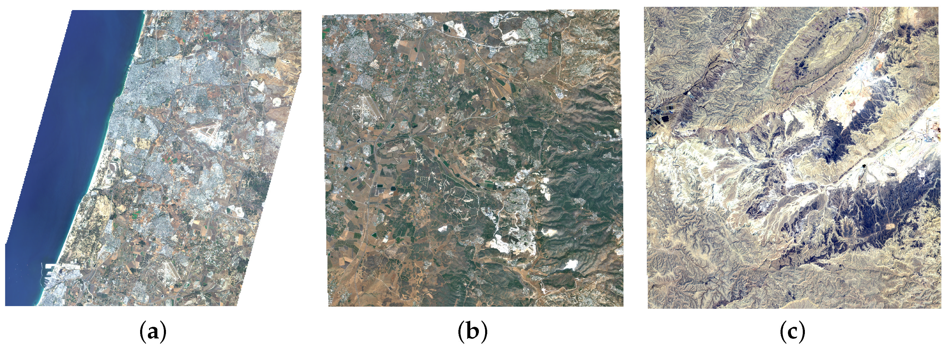
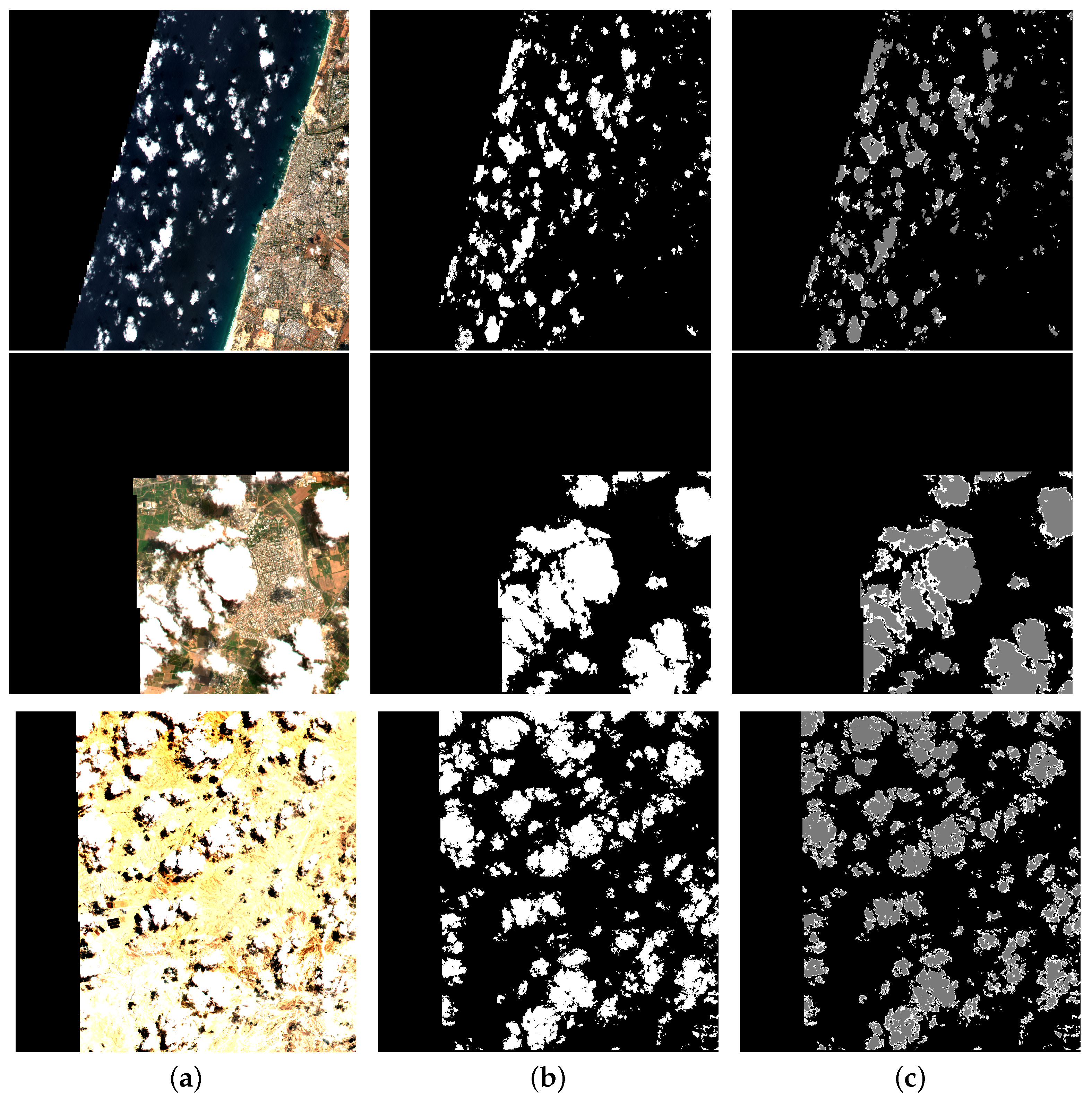
The experimental dataset used in this study had to be created manually in order to determine whether it was possible to obtain better cloud masks for VEN μ S satellite data using CNNs. Three VEN μ S tiles were chosen for be labelling: W07, S01, and S05 (see Figure 1 and Figure 2). These sites were considered to contain at least a small portion of each of the main land cover types appearing in Israel, that is, vegetated areas, urban areas, agricultural areas, water bodies, and arid areas, while leaving most of their variations unseen for later utterly independent experiments. Nine tiles from scenes spanning April to August 2018 and 2019 were manually labelled for these sites. In order to pay attention to the above-mentioned problematic arid land cover classes, more than a half of the dataset consisted of scenes from the Negev desert (tile S05). A comparison of cloud masks generated by MAJA and labels created manually is illustrated in Figure 3.
Two datasets were generated. The first included thin and thick clouds as well as clear pixels, while the second included only a binary mask with either clear or cloudy pixels, as detailed in the list below and depicted in Figure 4.
1.
Three-class dataset: thick clouds, thin clouds, cloudless
  • thick cloud: an absolutely non-transparent cloud pixel;
  • thin cloud: a pixel corrupted by a semi-transparent cloud;
  • cloudless: clear and cloud-free pixels.
2.
Binary class dataset: clouds, cloudless
  • a derived product from the three-class dataset created by joining the two cloud classes (thick and thin) into one.
For each of the above-listed labelled datasets, three sets of input bands were used:
1
VEN μ S scenes containing all spectral bands (see Table 1);
2
RGB VEN μ S scenes;
3
RGB + NDVI VEN μ S scenes.
These labelling and input band variations allowed to test the performance of CNNs on VEN μ S data depending on whether the classification is binary or multi-class as well as to make inferences about their utility in any other satellite data source containing at least red, green, and blue bands, making the results as general as possible. The third band variation containing RGB enhanced by the normalized difference vegetation index (NDVI) was added as an exemplary study of whether NDVI helps the CNN models to improve their prediction; this was carried out in order to test such claims [39] and to test its effect, especially over the desert land type with extremely sparse vegetation.
Manual labelling was carried out using the labelling tool developed as part of [40] and provided through the official university website (https://dspace.cvut.cz/handle/10467/95456, accessed on 11 October 2022). As all the other versions of the dataset are only derived products of the full-band multi-class one, only this one is provided to save space on the provider’s storage disks; it can be obtained online (https://zenodo.org/record/7040177, accessed on 11 October 2022) and is licensed with the Creative Commons Attributions 4.0 International license (https://creativecommons.org/licenses/by/4.0/legalcode, accessed on 11 October 2022).

3. Methodology

After the training datasets were created, as described in Section 2, tested architectures were chosen. Their choice and description can be found in Section 3.1. Seventy percent of the dataset was then used for training and thirty percent to validate the utilized architectures. The way the experiments were conducted is detailed in Section 3.2. The entire workflow is illustrated in Figure 5.

3.1. Architectures

Out of the four CNN architectures commonly employed for image segmentation in the field of remote sensing ([41,42]) as depicted in Figure 6, three were chosen for implementation. The architectures were chosen based on their utilization as backbone models in the CNN-based cloud cover studies mentioned in Section 1. As far as possible, all of them are used in their original settings, and are therefore described only briefly.
The fundamental goal of the CNN architectures examined here is to perform semantic segmentation. They are based on the encoder–decoder structure, the most common structure for image segmentation [42]. The encoder maps every given input x X R d 0 to a feature space z Z R d κ , and this feature map then serves as an input for the decoder to produce an output y Y R d 0 , where κ denotes the depth of the network [43]. A more illustrative depiction of this idea can be seen in Figure 7.
All architectures were enhanced by an option to include dropout layers [44] after each batch normalization layer to test the dropout effect on overfitting, as used in [45]. Otherwise, they were used in their original setting.

3.1.1. U-Net

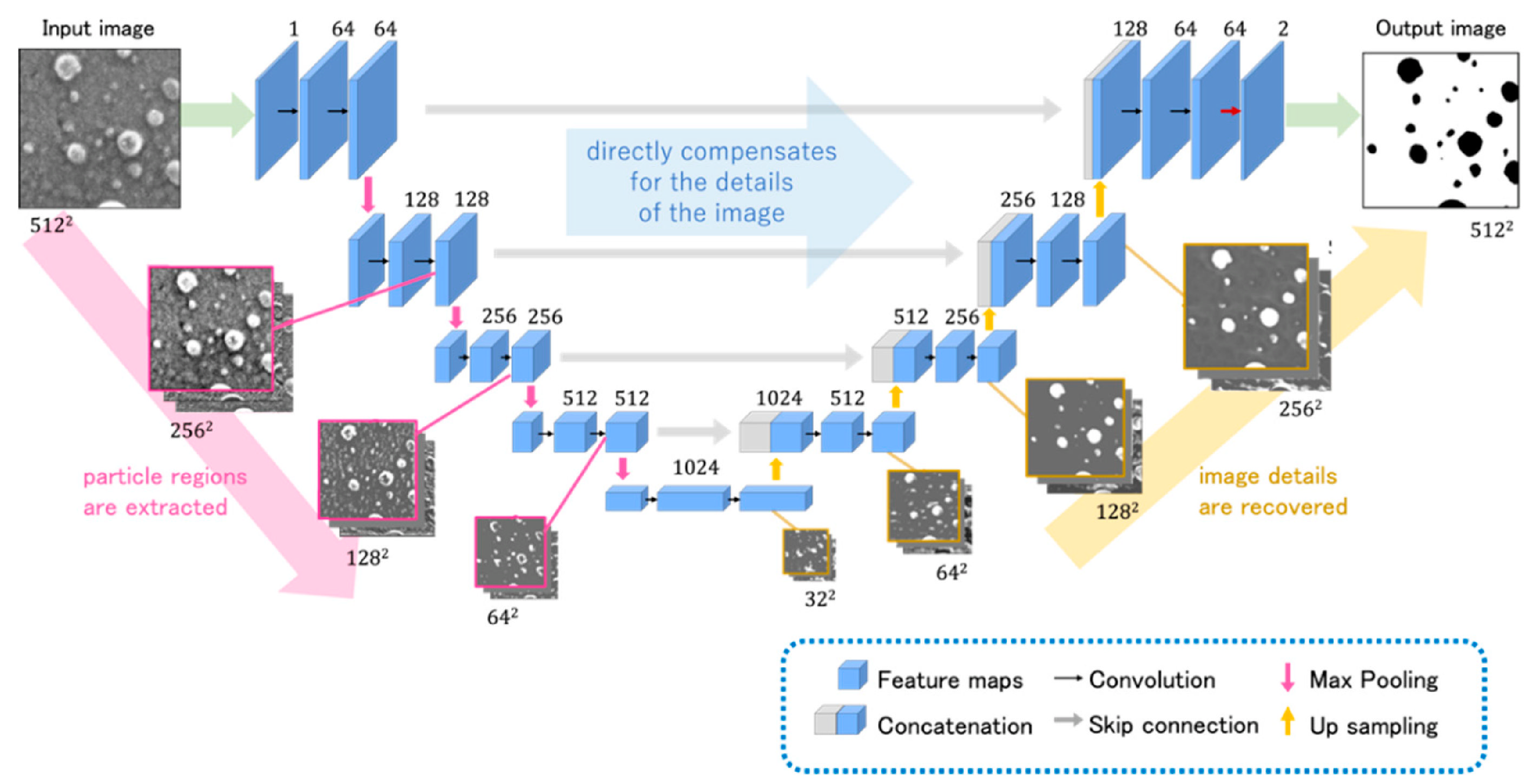
Although U-Net was initially designed to segment neuronal structures in electron microscopy images [21], the architecture quickly established itself as the state-of-the-art model in computer vision, including remote sensing [42]. It is, as depicted in Figure 8, a symmetric U-shaped (hence the name) five-level encoder–decoder [43] CNN using skip connections built upon a fully convolutional network (FCN) [46]. In an addition to FCN, the decoder contains a large number of feature channels symmetrical to corresponding encoder layers, allowing the model to propagate context information to higher resolution layers; these corresponding levels are connected by skip connections transferring the entire feature maps. All fully connected layers of the FCN are dropped, making the model much lighter in terms of the required parameters.
The total number of parameters of the U-Net architecture used for the full-band dataset in this study was 31,060,546, out of which 31,048,770 were trainable.

3.1.2. SegNet

SegNet [48] is a symmetrical U-shaped encoder–decoder [43] CNN, similar to U-Net in its core. As can be seen in Figure 9, there are three differences from U-Net. First, there is an extra lowest-level convolutional block. Second, the portion of convolutional blocks within one level is one layer deeper. The biggest difference lies in the design of skip layers; in U-Net, they propagate entire feature maps to be concatenated with the upsampling layers’ output, whereas in SegNet they transfer only pooling indices, which are then used for upsampling. The memory saved in the skip connections allows the use of extra layers and convolutional blocks when compared to U-Net.
The total number of parameters of the SegNet architecture used for the full-band dataset in this study was 62,502,530, out of which 62,481,538 were trainable.

3.1.3. DeepLabv3+

An alternative to common convolution is atrous (sparse) convolution. The advantage of this approach lies in the ability to enlarge the receptive field via dilation while keeping the same number of parameters, generally resulting in architectures with fewer parameters. Atrous convolutions have been used in the task of cloud detection both in the field of remote sensing, such as [22], who used atrous convolutions in U-Net, and in other fields, such as [49]. One of the models using atrous convolutions while serving as a backbone for many other networks is DeepLab.
The architecture known as DeepLab is available in many generations. The first generation [50] merely utilized the idea of atrous convolutions in its architecture; the second generation [28] expanded this design into atrous spatial pyramid pooling (ASPP) and experimented with ResNet [51] as its backbone architecture; and the third generation [52] augmented the ASPP module with image-level features to capture global context [53] and included batch normalization layers [54]. Finally, the DeepLabv3+ [55] generation used DeepLabv3 as the encoder following the encoder–decoder paradigm [43], resulting in segmentation refinement, especially at object borders. DeepLabv3+ is the generation implemented in this study.
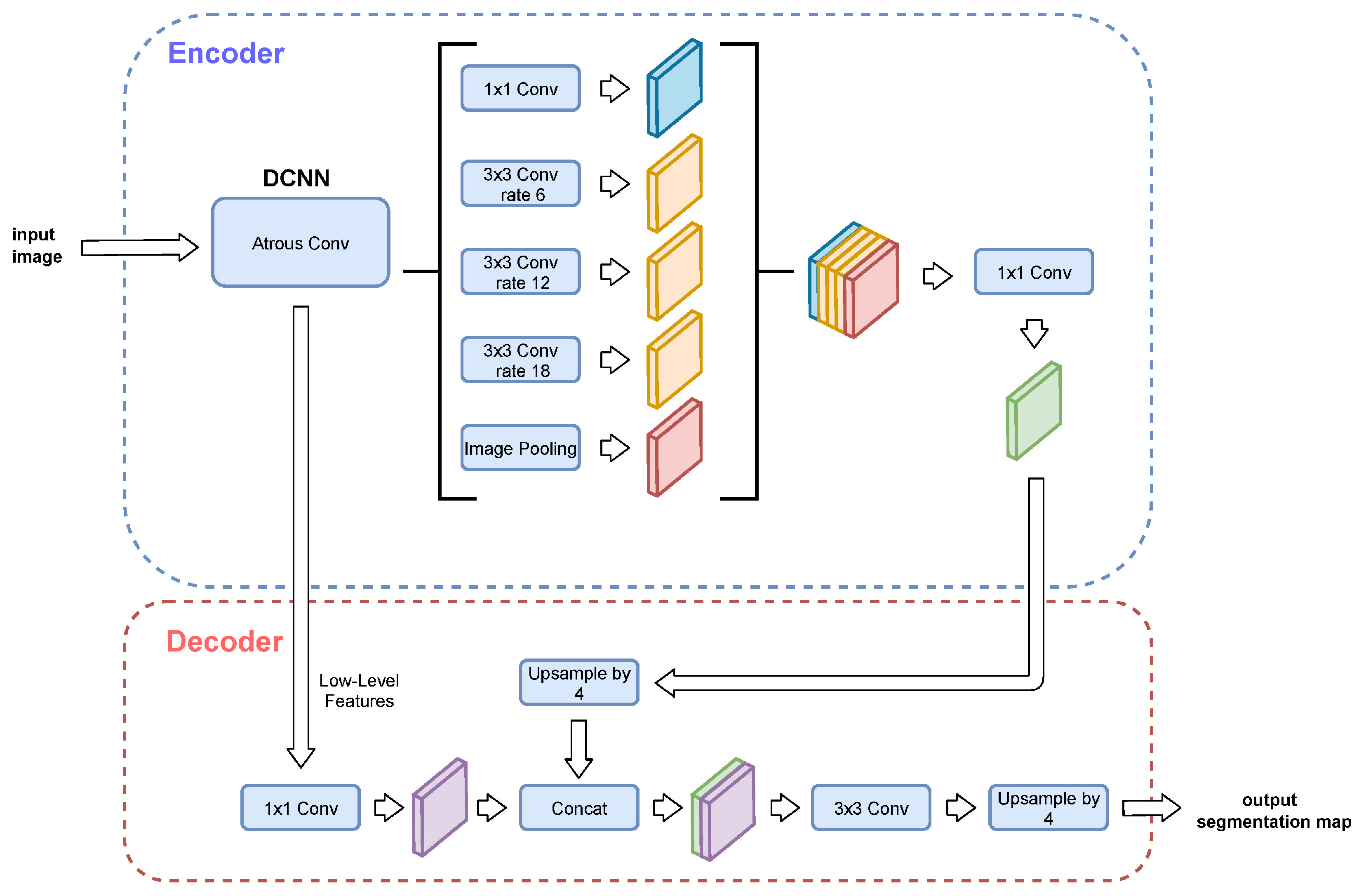
As a result, DeepLabv3+ consists of multiple stages. The first stage of the encoder is a backbone architecture, a CNN without its classification layers. The authors of the original paper experimented with ResNet and Xception [56] as backbone architectures; in this research, it is represented by ResNet-50, ResNet-101, and ResNet-152. The second stage of the encoder is the ASPP applied on the output of the backbone architecture, followed by an atrous separable convolution. The decoder consists first of a concatenation of the atrous separable convolution output and a convoluted low-level output from the backbone architecture, and second of convolutional blocks and upsampling, as illustrated in Figure 10.
The total number of parameters in the DeepLabV3+ architecture used for the full-band dataset in this study is as follows, divided by the three backbones:
  • ResNet-50: 17,860,786, out of which 17,826,002 were trainable
  • ResNet-101: 36,931,250, out of which 36,844,242 were trainable
  • ResNet-152: 52,644,018, out of which 52,510,930 were trainable

3.2. Experiments

3.2.1. Experiment Settings

In order to receive both training and validation samples from every tile in the dataset, patches of size 1024 × 1024 were used in the experiments, resulting in 72 patches (four patches per each of 2048 × 2048 tiles); 70% of such patches were used for training and the rest served to validate the model, always using at least one patch from a tile in the validation section. Every training ran for at most 1000 epochs, with models being saved only when reaching a lower validation loss value than in the previous best epoch. The patience of 100 epochs for early stopping was used to avoid overfitting; if the validation loss value did not decrease for 100 epochs, the training was stopped. As the activation function for the convolutional layers, the rectified linear unit (ReLU) function was chosen, as it is widely used in deep learning [58]. Batch normalization layers were used after activation layers.
Every architecture ran twice on each dataset (see Section 2), once without the utilization of dropout layers and once with dropout layers, with a rate of 0.5 (50%) following every batch normalization layer. Moreover, the impact of simple data augmentation was tracked; every training run was first performed only with the original dataset, then repeated using data enhanced by their rotations (by 90, 180, and 270 degrees, resulting in a dataset four times bigger than the original one).
The results for all the described settings are presented in Section 4.

3.2.2. Loss Functions

To evaluate the performance of the trained models, binary cross entropy and Dice loss were used for the binary and multi-class datasets, respectively.
The cross entropy is the average number of bits needed to encode data from a source with a distribution q while using model p [59]. Using it as a loss function for two classes, the goal is to minimize the Kullback–Leibler divergence [60]. Mathematically, the loss function can be described as follows:
H q ( p ) = 1 1 N i = 1 N ( y i l o g ( p ( y i ) ) + ( 1 y i ) l o g ( 1 p ( y i ) ) ) ,
where H q ( p ) is the binary cross entropy loss, N is the number of training/validation samples, y i is the ground-truth label, and p ( y i ) is the predicted probability of the sample having the ground-truth value.
Using Dice loss, the user wants to minimize the so-called Sørensen–Dice coefficient, which is a measure of the association between compared classes defined for two classes as a ratio of twice the common area of two sets to the sum of the cardinalities of the sets [61]. Its use in ANNs and semantic segmentation began in the 1990s, e.g., in [62]. Dice loss was used for the multi-class dataset because it computes the loss function relatively for each class instead of working with the absolute number of pixels per class, helping to lower the effect of imbalanced classes. Mathematically, the Sørensen–Dice coefficient can be described as follows:
D = 2 i N g i p i i N g i 2 + i N p i 2 ,
where D is the Sørensen–Dice coefficient, N is the number of training/validation samples, g i is the count of ground-truth pixels for sample i, and p i is the count of predicted pixels for sample i.

4. Results

The results for all settings for both the multi-class and binary datasets are presented in Table 2 and Table 3, respectively. All loss function values reported in the tables and all figures in this chapter were computed over the independent validation set, as described in Section 3.2.
It is apparent from the tables that the results from the binary classification are much more accurate. This finding indicates that most errors in Table 2 are due to inadequate differentiation between thick and thin clouds instead of from the problem of cloud vs. cloud-free pixels. This issue was anticipated, as the border between these two classes is not very clear and there could be different ground-truth labels for pixels with the same spectral reflectance in the training dataset due to human error.
Section 4.1 looks at the results from the architecture point of view, Section 4.2 examines the results obtained with different datasets, and Section 4.3 compares the results obtained in this study with cloud masks obtained by MAJA [12].

4.1. Comparison among Architectures

Comparing the loss values of U-Net, SegNet, and multiple variations of DeepLabV3+ reported in Table 2 and Table 3, U-Net shows the best results for almost every setting. The few minor exceptions are assumed to be caused by bad initial random values of the weights on account of their rarity.
Another finding is that using dropout layers with a rate of 0.5 (50%) actually led to higher loss value in 82% of the times, and therefore to lower accuracy, which was in contrast to the expected behaviour. Furthermore, dropout did not help to increase the performance of SegNet. Although dropout layers are used in many papers to avoid overfitting ([19,45,63,64,65]), comparing performance with and without dropout is not common. Hence, this finding points out that such an experiment should be considered when testing a new architecture.
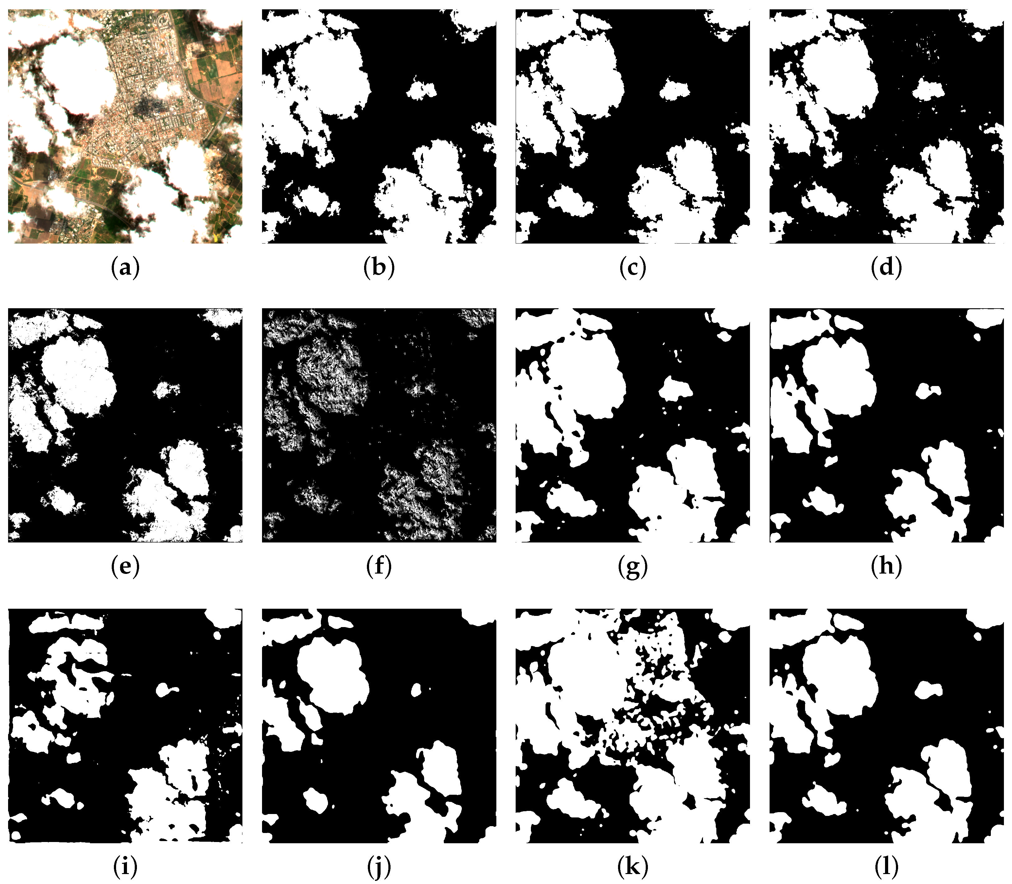
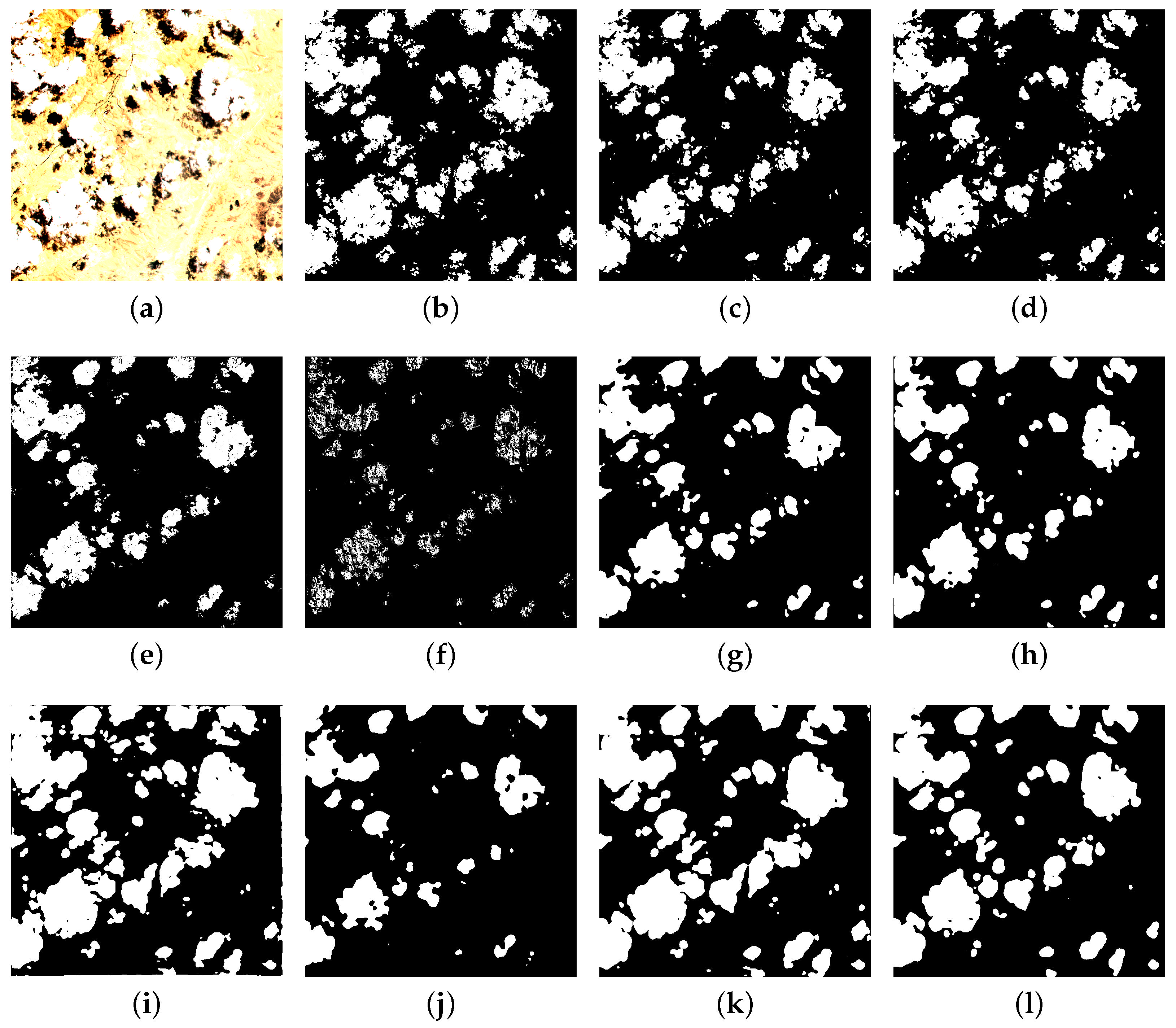
Examples of the detection performance are presented in Figure 11 and Figure 12. Visual inspection of the results leads to the same conclusion as above, with U-Net performing the best among the chosen architectures. DeepLabV3+ usually smoothens detected clouds too much (additionally, DeepLabV3+ with ResNet-152 as the backbone model apparently has a problem with urban areas, as depicted in Figure 12k). Meanwhile, SegNet underpredicts cloud areas, especially thinner and smaller ones. U-Net seems to miss a few extra small cloud patches, and otherwise corresponds with the ground-truth label very well. Visual inspection reveals that the non-dropout version of SegNet consistently outperformed the dropout one because the results returned when using dropout layers are too crispy and scattered. However, all architectures seem to deal well with holes in clouds, and to be similarly prone to the more challenging land covers such as urban and arid areas, as illustrated in Figure 11 and Figure 12, respectively.

4.2. Comparison among Datasets

Comparing loss values over different datasets, a conclusion that extra bands or indices treated as bands are valuable for the cloud detection model performance can be drawn with an appropriate degree of caution. There are only two examples in which a model trained on an RGB dataset performed better than the others for the multi-class problem, and only three for the binary problem, as reported in Table 2 and Table 3, respectively. However, when comparing RGB to the results for RGB enhanced by the NDVI, the results are slightly in favour of pure RGB (lower loss value in 55%).
The original expectation from the effect of data augmentation was to lower the loss function in almost all cases. However, it helped to get a lower loss function value in twelve cases out of thirty for the multi-class dataset and fourteen cases out of thirty for the binary one. A possible reason for such behaviour could be that the clouds over Israel are not direction-independent; as most of the clouds in Israel originate from the Mediterranean Sea, this could be a conceivable explanation.
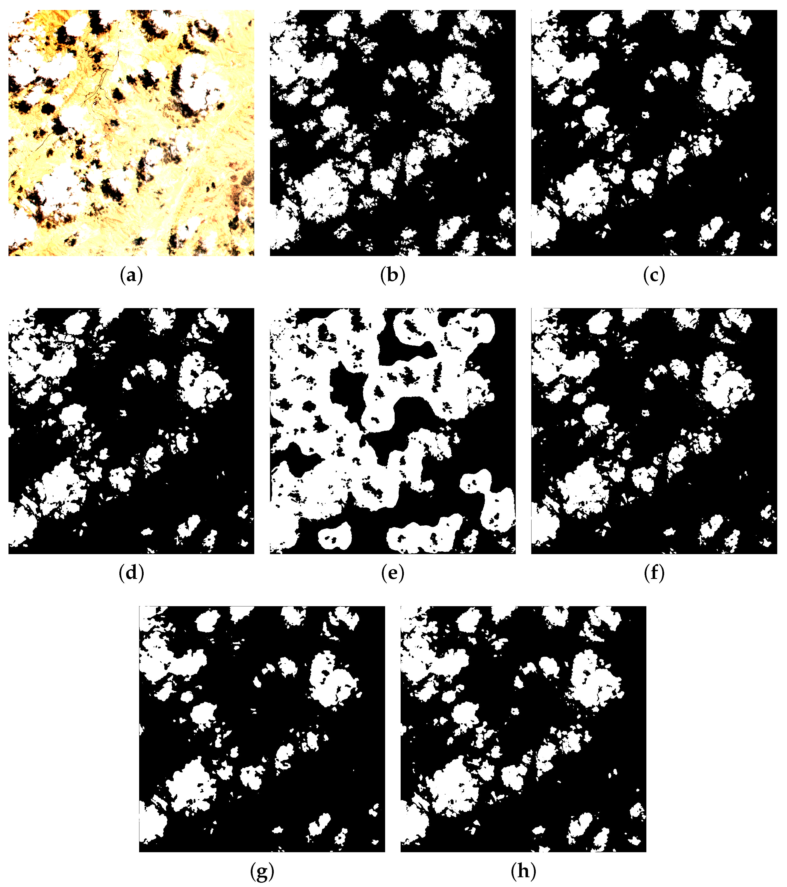
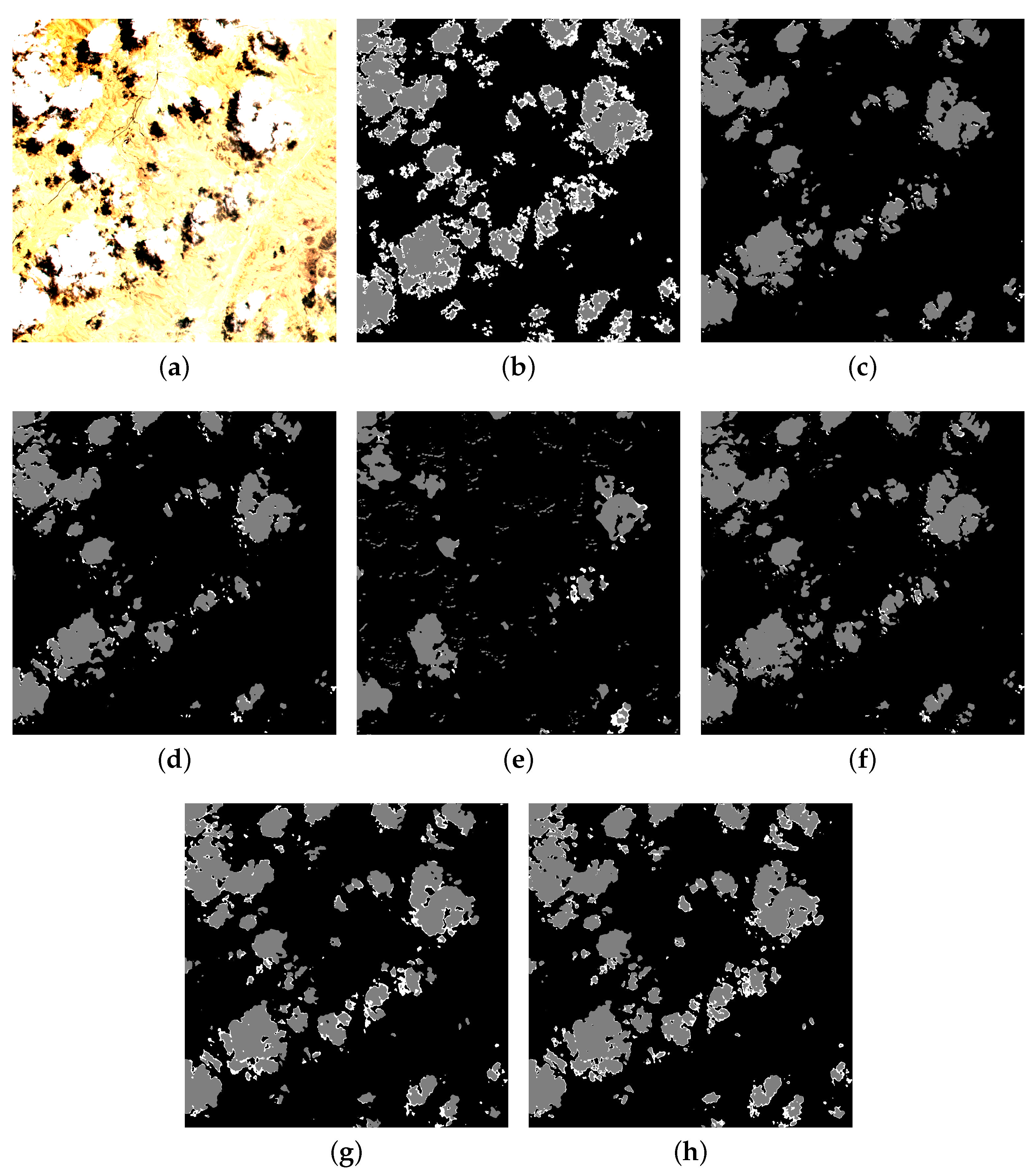
Visual inspection of the results leads to a few findings. As shown in Figure 13, the binary classifier running on the RGB + NDVI dataset suffers a great deal of overdetection in arid areas. As the loss value according to Table 3 is not high, it performs well in non-arid areas; an experiment focusing mainly on the influence of NDVI or other indices such as the crust index [66] on cloud detection over arid areas could be valuable. For the multi-class version illustrated in Figure 14, the overdetection is not as extreme; however, the model nonetheless expects many small scattered cloud patches where either no clouds appear or parts of bigger clouds should be.
Another observation from the visual results is that data augmentation solves the aforementioned issue mentioned, as it is able balance differences between different architectures. It is especially helpful for thin cloud detection, which seems to be very unsuccessful for arid areas, and worked particularly well for the RGB + NDVI dataset, as can be seen in Figure 14.

4.3. Comparison with MAJA

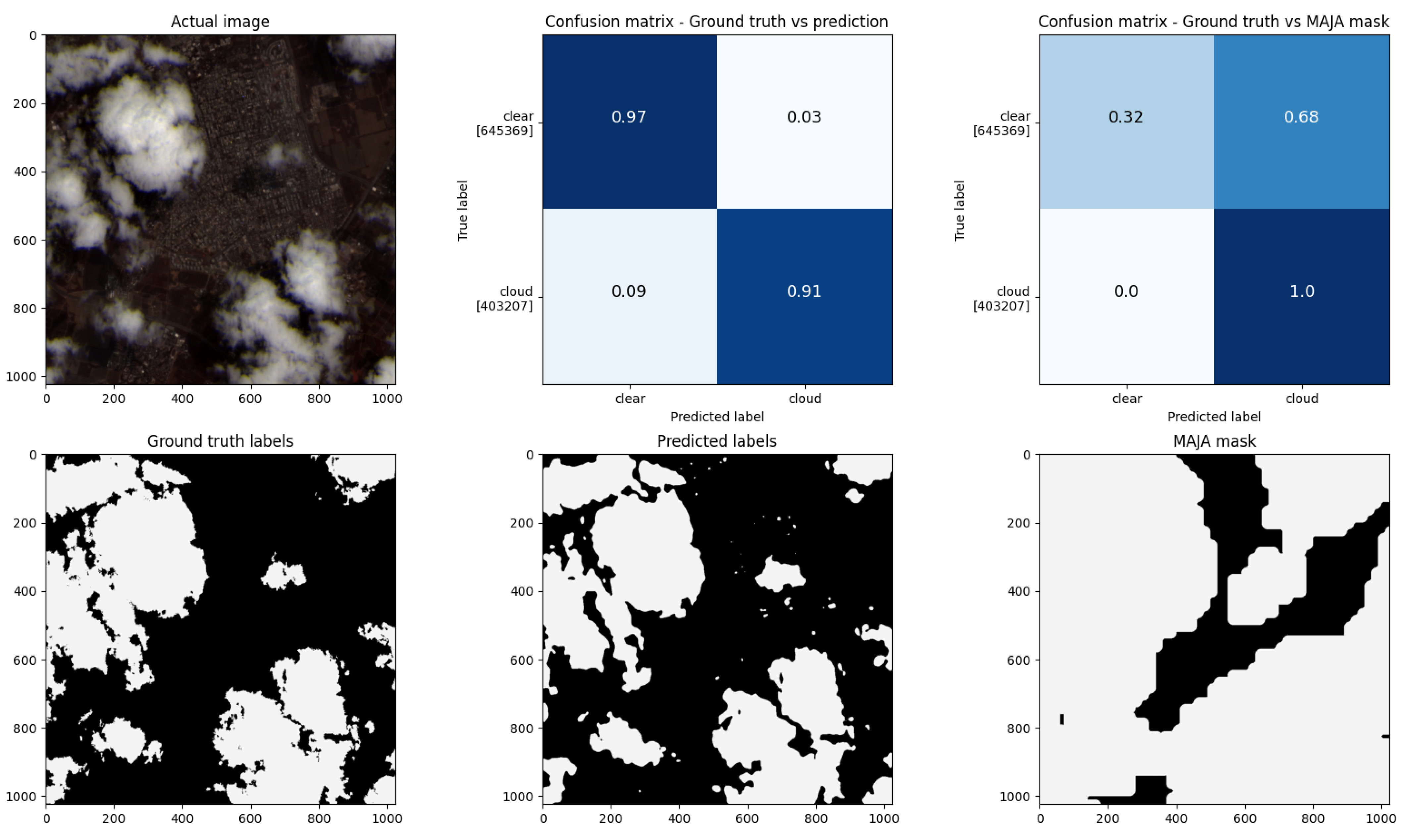
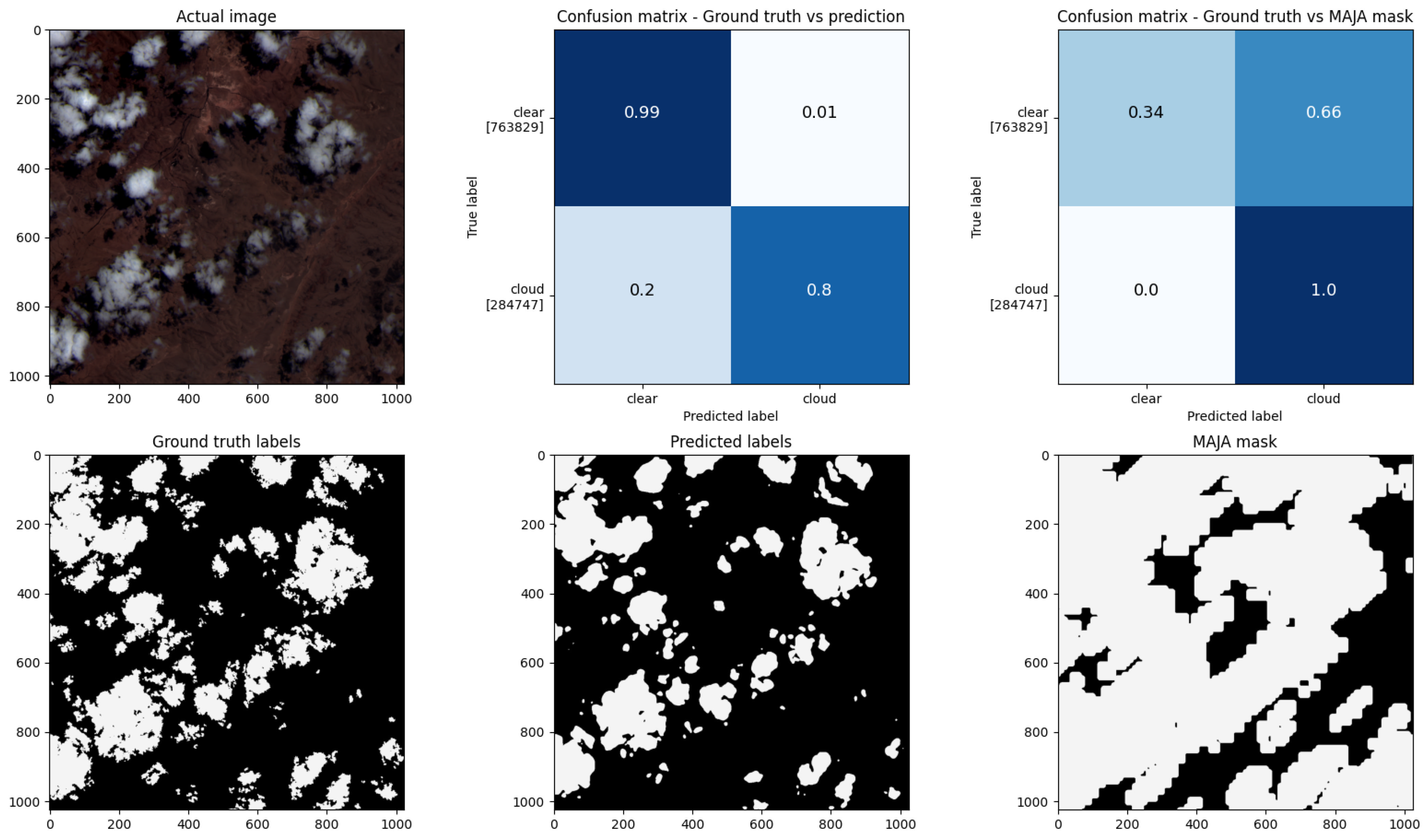
As illustrated in Figure 15 and Figure 16, visual comparison of MAJA-based cloud masks and the results obtained by U-Net favours U-Net. MAJA masks tend to suffer from considerable overestimation of cloud-covered areas.
Comparison of confusion matrices reported in Figure 15 and Figure 16 supports this claim, showing that although 100% of cloud-covered pixels are labelled as cloudy on MAJA masks, more than 65% of the cloud-free pixels are usually considered to be cloudy as well; this mislabelling radically reduces the number of applicable products offered to the user. Although U-Net misses a few cloudy pixels, its mislabelling is minimal, never reaching the level of 5%.

5. Discussion

This study describes a new cloud mask methodology for VEN μ S images and conducts research utilizing this task to test the most common CNN architectures for semantic segmentation. U-Net attained the best results among the tested architectures, outperforming the current default algorithm MAJA by tens of percents in terms of lowering the false positive prediction and having few problems with the challenging arid terrain in southern Israel. Its main strength was shown to be in differentiating between clouds and non-cloud pixels, whereas in the case of thick cloud vs. thin cloud differentiation, it evidently prefers the thick cloud class. Nevertheless, this behaviour does not necessarily mean that the performance of CNNs is worse for thin clouds, as this could be caused by ground truth label imperfection or class imbalance.
In addition, we conducted research exploring the effect of dropout layers and data augmentation. Dropout layers were found to be an advantage in only 25% of cases, and data augmentation in slightly more than one third of cases. This finding hints that other experiments should pay attention to these tools. An experiment dealing with the effect of data augmentation on spatially dependent features could be valuable.
Additionally, the influence of different band sets on the performance of CNN models was investigated. It was found that in most cases a model trained on full-band VEN μ S images reached better results than reduced sets. Indices such as NDVI proved their strength in cloud detection, and a corresponding analysis could be helpful in the task of cloud detection. Despite this finding, the model’s performance over a simple RGB dataset was valuable, and outperformed default MAJA masks, leading to the conclusion that the proposed model could be useful even for data sources screening only the visible spectrum.
However, the fact that all of the CNN architectures used in this study improved the cloud mask accuracy does not mean that their usage is without drawbacks. The nature of CNNs is that they work as ’black boxes’, and although user experience can help to foresee the network’s behaviour, it is believed to be impossible to understand and appropriately trust the meaning of millions of their parameters. In recent years, explainable artificial intelligence has been used to deal with this complication [67], and would be a valuable enhancement for any continuation of deep learning-based cloud detection. Another issue is the fact that neural networks generally have extremely high data requirements. Although there is an open dataset provided with this article to fight this difficulty, models trained on this dataset can perform slightly worse on data coming from other satellite systems or other locations, as they may not have seen relevant backgrounds (e.g., high latitude or high altitude areas) before and because even the RGB-surveying satellites differ slightly in their use of central bandwidths. Another problem is connected to the dataset used in this study, which includes only limited types of clouds that appeared in the areas of interest during the chosen period. As such, its performance on different cloud types, such as cirrus clouds, has not been tested. The final downsides that should be mentioned are the time and resources requirements of the models; it took three days to train U-Net on thirty CPU cores, while it took only one hour on a Tesla V100 GPU.

6. Conclusions

Cloud cover has always been an obstacle for many tasks in remote sensing. For certain satellite systems, there are numerous approaches to detect and mask cloud-corrupted pixels; however, this is not the case with the VEN μ S satellite system. The current algorithm used to obtain cloud masks for VEN μ S scenes is MAJA. Using sample zones selected in Israel, this paper shows MAJA’s insufficiency and tendency to extensively overestimate the cloud cover, especially in urban regions and in the almost exclusively arid southern parts of the country.
Recent research on CNNs has shown promising results in cloud cover detection, making them candidates for increasing cloud mask quality. Although all cited papers proposing CNN-based cloud detection have claimed to outperform all the other tested methods, only half of them were compared to other CNNs. This lack of comparison makes the choice of a model challenging for remote sensing scientists with no experience with CNNs. This paper can serve as such a benchmark. It explores the cloud detection performance of a selection of the most common CNN architectures while lowering the false positive detection ratio by tens of percents when compared to the MAJA algorithm. Moreover, it investigates their performance over different settings, including diverse numbers of classes (binary vs. multiclass), diverse band and index variations (RGB vs. RGB + NIR vs. full-band), and the effect of overfitting avoidance strategies (dropout, data augmentation). Our results show that U-Net is the best-performing architecture among the most common basic CNNs. Its accuracy over difficult land cover types such as deserts and its performance over a simple RGB dataset illustrate its potential for other satellite systems.
Where possible, this paper is being published under open science principles [68]; the code (https://github.com/pesekon2/cloud-detection-venus, accessed on 11 October 2022) and data (https://zenodo.org/record/7040177, accessed on 11 October 2022) used in this study are freely accessible under the MIT license (https://opensource.org/licenses/MIT, accessed on 11 October 2022) and the Creative Commons Attributions 4.0 International license (https://creativecommons.org/licenses/by/4.0/legalcode accessed on 11 October 2022), respectively.

Author Contributions

Conceptualization, O.P., A.K., M.S.-R.; methodology, O.P.; software, O.P.; validation, O.P.; formal analysis, O.P.; investigation, O.P.; resources, O.P., A.K.; data curation, O.P.; writing—original draft preparation, O.P., A.K.; writing—review and editing, O.P., A.K., M.S.-R.; visualization, O.P., A.K.; supervision, A.K., M.S.-R.; project administration, A.K. All authors have read and agreed to the published version of the manuscript.

Funding

This work was supported by the Grant Agency of the Czech Technical University in Prague, grant No. SGS22/047/OHK1/1T/11.

Data Availability Statement

The data presented in this study are openly available at https://zenodo.org/record/7040177 accessed on 11 October 2022 at DOI:10.5281/zenodo.7040177.

Conflicts of Interest

The authors declare no conflict of interest.

Abbreviations

The following abbreviations are used in this manuscript:
ACCAAutomated Cloud Cover Assessment
CNNConvolutional Neural Network
FCNFully Convolutional Network
FmaskFunction of Mask
LEDAPSLandsat Ecosystem Disturbance Adaptive Processing System
MAJAMACCS-ATCOR Joint Algorithm
NDVINormalized Difference Vegetation Index
ReLURectified Linear Unit
RGBRed, Green, Blue
VEN μ SVegetation and Environment New Micro-Satellite
XBAER-CMeXtensible Bremen AErosol Retrieval

References

  1. King, M.D.; Platnick, S.; Menzel, W.P.; Ackerman, S.A.; Hubanks, P.A. Spatial and Temporal Distribution of Clouds Observed by MODIS Onboard the Terra and Aqua Satellites. IEEE Trans. Geosci. Remote Sens. 2013, 51, 3826–3852. [Google Scholar] [CrossRef]
  2. Rossow, W.B.; Schiffer, R.A. Advances in Understanding Clouds from ISCCP. Bull. Am. Meteoroligcal Soc. 1999, 80, 2261–2288. [Google Scholar] [CrossRef]
  3. Asner, G.P. Cloud Cover in Landsat Observations of the Brazilian Amazon. Int. J. Remote Sens. 2001, 22, 3855–3862. [Google Scholar] [CrossRef]
  4. Irish, R. Landsat 7 Automatic Cloud Cover Assessment. In Algorithms for Multispectral, Hyperspectral, and Ultraspectral Imagery VI; SPIE: Bellingham, WA, USA, 2000. [Google Scholar]
  5. Zhu, Z.; Woodcock, C.E. Object-Based Cloud and Cloud Shadow Detection in Landsat Imagery. Remote Sens. Environ. 2012, 118, 83–94. [Google Scholar] [CrossRef]
  6. Koren, I.; Remer, L.A.; Kaufman, Y.J.; Rudich, Y.; Martins, J.V. On the Twilight Zone Between Clouds and Aerosols. Geophys. Res. Lett. 2007, 34. [Google Scholar] [CrossRef] [Green Version]
  7. Hollingsworth, B.V.; Chen, L.; Reichenbach, S.E.; Irish, R.R. Automated Cloud Cover Assessment for Landsat TM Images. In Imaging Spectrometry; SPIE: Bellingham, WA, USA, 1996. [Google Scholar]
  8. Vermote, E.; Saleous, N. LEDAPS Surface Reflectance Product Description; University of Maryland: College Park, MD, USA, 2007. [Google Scholar]
  9. Main-Knorn, M.; Pflug, B.; Louis, J.; Debaecker, V.; Müller-Wilm, U.; Gascon, F. Sen2Cor for Sentinel-2. Image Signal Process. Remote Sens. 2017, 10427, 37–48. [Google Scholar]
  10. Zhu, Z.; Wang, S.; Woodcock, C.E. Improvement and Expansion of the Fmask Algorithm: Cloud, Cloud Shadow, and Snow Detection for Landsats 4–7, 8, and Sentinel 2 Images. Remote Sens. Environ. 2015, 159, 269–277. [Google Scholar] [CrossRef]
  11. Mei, L.; Vountas, M.; Gómez-Chova, L.; Rozanov, V.; Jäger, M.; Lotz, W.; Burrows, J.P.; Hollman, R. A Cloud Masking Algorithm for the XBAER Aerosol Retrieval Using MERIS Data. Remote Sens. Environ. 2016, 197, 37–48. [Google Scholar] [CrossRef]
  12. Hagolle, O.; Huc, M.; Pascual, D.V.; Dedieu, G. A Multi-Temporal Method for Cloud Detection, Applied to FORMOSAT-2, VENµS, LANDSAT and SENTINEL-2 Images. Remote Sens. Environ. 2010, 114, 1747–1755. [Google Scholar] [CrossRef] [Green Version]
  13. Zhu, Z.; Woodcock, C.E. Automated Cloud, Cloud Shadow, and Snow Detection in Multitemporal Landsat Data: An Algorithm Designed Specifically for Monitoring Land Cover Change. Remote Sens. Environ. 2014, 152, 217–234. [Google Scholar] [CrossRef]
  14. Razavian, A.S.; Azizpour, H.; Sullivan, J.; Carlsson, S. CNN Features Off-the-Shelf: An Astounding Baseline for Recognition. In Proceedings of the IEEE Conference on Computer Vision and Pattern Recognition, Columbus, OH, USA, 23–28 June 2014. [Google Scholar]
  15. Chen, Y.; Fan, R.; Bilal, M.; Yang, X.; Wang, J.; Li, W. Multilevel Cloud Detection for High-Resolution Remote Sensing Imagery Using Multiple Convolutional Neural Networks. ISPRS Int. J.-Geo-Inf. 2018, 7, 181. [Google Scholar] [CrossRef]
  16. Ma, N.; Sun, L.; Zhou, C.; He, Y. Cloud Detection Algorithm for Multi-Satellite Remote Sensing Imagery Based on a Spectral Library and 1D Convolutional Neural Network. Remote Sens. 2021, 16, 3319. [Google Scholar] [CrossRef]
  17. Shi, M.; Xie, F.; Zi, Y.; Yin, J. Cloud Detection of Remote Sensing Images by Deep Learning. In Proceedings of the 2016 International Geoscience and Remote Sensing Symposium IGARSS, Beijing, China, 10–15 July 2016; pp. 701–704. [Google Scholar]
  18. Li, Z.; Shen, H.; Cheng, Q.; Liu, Y.; You, S.; He, Z. Deep Learning Based Cloud Detection for Medium and High Resolution Remote Sensing Images of Different Sensors. ISPRS J. Photogramm. Remote Sens. 2019, 250, 197–212. [Google Scholar] [CrossRef] [Green Version]
  19. Xie, F.; Shi, M.; Shi, Z.; Yin, J.; Zhao, D. Multilevel Cloud Detection in Remote Sensing Images Based on Deep Learning. IEEE J. Sel. Top. Appl. Earth Obs. Remote Sens. 2017, 8, 3631–3640. [Google Scholar] [CrossRef]
  20. Francis, A.; Sidiropoulos, P.; Muller, J. CloudFCN: Accurate and Robust Cloud Detection for Satellite Imagery with Deep Learning. Remote Sens. 2019, 11, 2312. [Google Scholar] [CrossRef] [Green Version]
  21. Ronneberger, O.; Fischer, P.; Brox, T. U-Net: Convolutional Networks for Biomedical Image Segmentation. In Proceedings of the International Conference on Medical Image Computing and Computer-Assisted Intervention (MICCAI), Munich, Germany, 5–9 October 2015; Navab, N., Hornegger, J., Wells, W.M., Frangi, A.F., Eds.; Medical Image Computing and Computer-Assisted Intervention, Pt III. Springer: Cham, Switzerland, 2015. [Google Scholar]
  22. Li, X.; Yang, X.; Li, X.; Lu, S.; Ye, Y.; Ban, Y. GCDB-UNet: A Novel Robust Cloud Detection Approach for Remote Sensing. Knowl.-Baed Syst. 2022, 238, 107890. [Google Scholar] [CrossRef]
  23. Wu, X.; Shi, Z. Utilizing Multilevel Features for Cloud Detection on Satellite Imagery. Remote Sens. 2018, 10, 1853. [Google Scholar] [CrossRef] [Green Version]
  24. Simonyan, K.; Zisserman, A. Very Deep Convolutional Networks for Large-Scale Image Recognition. 2014. Available online: http://arxiv.org/abs/1409.1556 (accessed on 6 February 2022).
  25. Krizhevsky, A.; Sutskever, I.; Hinton, G.E. ImageNet Classification with Deep Convolutional Neural Networks. Adv. Neural Inf. Process. Syst. (NIPS) 2012, 60, 1097–1105. [Google Scholar] [CrossRef] [Green Version]
  26. Zhao, R.; Ouyang, W.; Li, H.; Wang, X. Saliency Detection by Multi-Context Deep Learning. In Proceedings of the IEEE Conference on Computer Vision and Pattern Recognition (CVPR), Boston, MA, USA, 7–12 June 2015; pp. 1265–1274. [Google Scholar]
  27. Zhan, Y.; Wang, J.; Shi, J.; Cheng, G.; Yao, L.; Sun, W. Distinguishing Cloud and Snow in Satellite Images via Deep Convolutional Network. IEEE Geosci. Remote. Sens. Lett. 2017, 14, 1785–1789. [Google Scholar] [CrossRef]
  28. Chen, L.C.; Papandreou, G.; Kokkinos, I.; Murphy, K.; Yuille, A.L. DeepLab: Semantic Image Segmentation with Deep Convolutional Nets, Atrous Convolution, and Fully Connected CRFs. arXiv 2017, arXiv:1606.00915. Available online: https://arxiv.org/abs/1606.00915 (accessed on 11 October 2022).
  29. Sanchez, A.H.; Picoli, M.C.A.; Camara, G.; Andrade, P.R.; Chaves, M.E.D.; Lechler, S.; Soares, A.R.; Marujo, R.E.B.; Simbes, R.E.O.; et al.; Queiroz, G.R. Comparison of Cloud Cover Detection Algorithms on Sentinel-2 Images of the Amazon Tropical Forest. Remote Sens. 2020, 12, 1284. [Google Scholar] [CrossRef] [Green Version]
  30. Fernandez-Moran, R.; Gomez-Chova, L.; Alonso, L.; Mateo-Garcia, G.; Lopez-Puigdollers, D. Towards a Novel Approach for Sentinel-3 Synergistic OLCI/SLSTR Cloud and Cloud Shadow Detection Based on Stereo Cloud-Top Height Estimation. ISPRS J. Photogramm. Remote Sens. 2021, 181, 238–253. [Google Scholar] [CrossRef]
  31. Foga, S.; Scaramuzza, P.L.; Guo, S.; Zhu, Z.; Dilley, R.D.; Beckmann, T.; Schmidt, G.L.; Dwyer, J.L.; Hughes, M.J.; Laue, B. Cloud Detection Algorithm Comparison and Validation for Operational Landsat Data Products. Remote Sens. Environ. 2017, 194, 379–390. [Google Scholar] [CrossRef] [Green Version]
  32. Murino, L.; Amato, U.; Carfora, M.F.; Antoniadis, A.; Huang, B.; Menzel, W.P.; Serio, C. Cloud Detection of MODIS Multispectral Images. J. Atmos. Ocean. Technol. 2014, 31, 347–365. [Google Scholar]
  33. Jang, J.D.; Viau, A.A.; Anctil, F.; Bartholome, E. Neural Network Application for Cloud Detection in SPOT VEGETATION Images. Int. J. Remote Sens. 2006, 4, 719–736. [Google Scholar] [CrossRef]
  34. Dong, Z.P.; Liu, Y.X.; Xu, W.; Feng, Y.K.; Chen, Y.L.; Tang, Q.H. A Cloud Detection Method for GaoFen-6 Wide Field of View Imagery Based on the Spectrum and Variance of Superpixels. Int. J. Remote Sens. 2021, 16, 6315–6332. [Google Scholar]
  35. Segal-Rozenhaimer, M.; Li, A.; Das, K.; Chirayath, V. Cloud Detection Algorithm for Multi-Modal Satellite Imagery Using Convolutional Neural-Networks (CNN). Remote Sens. Environ. 2020, 237, 111446. [Google Scholar] [CrossRef]
  36. Houze, R.A. Types of Clouds in Earth’s Atmosphere. In Cloud Dynamics, 2nd ed.; Academic Press: Cambridge, MA, USA, 2014; pp. 3–23. [Google Scholar]
  37. Sun, L.; Wang, Q.; Zhou, X.Y.; Wei, J.; Yang, X.; Zhang, W.H.; Ma, N. A Priori Surface Reflectance-Based Cloud Shadow Detection Algorithm for Landsat 8 OLI. IEEE Geosci. Remote Sens. Lett. 2017, 10, 1610–1614. [Google Scholar] [CrossRef]
  38. Salvoldi, M.; Tubul, Y.; Karnieli, A. VENμS Derived NDVI and REIP at Different View Azimuth Angles. Remote Sens. 2022, 14, 184. [Google Scholar] [CrossRef]
  39. Lee, S.; Choi, J. Daytime Cloud Detection Algorithm Based on a Multitemporal Dataset for GK-2A Imagery. Remote Sens. 2021, 13, 3215. [Google Scholar] [CrossRef]
  40. Müller, V. Anotace MapovéHo Podkladu Podle SatelitníCh SníMků TeréNu. Master’s Thesis, Czech Technical University in Prague, Prague, Czech Republic, 2021. [Google Scholar]
  41. Hoeser, T.; Kuenzer, C. Object Detection and Image Segmentation with Deep Learning on Earth Observation Data: A Review-Part I: Evolution and Recent Trends. Remote Sens. 2020, 12, 1667. [Google Scholar] [CrossRef]
  42. Hoeser, T.; Bachofer, F.; Kuenzer, C. Object Detection and Image Segmentation with Deep Learning on Earth Observation Data: A Review-Part II: Applications. Remote Sens. 2020, 11, 3053. [Google Scholar] [CrossRef]
  43. Ye, J.C.; Sung, W.K. Understanding Geometry of Encoder-Decoder CNNs. In Proceedings of the Machine Learning Research, Long Beach, CA, USA, 9–15 June 2019; Chaudhuri, K., Salakhutdinov, R., Eds.; JMLR-Journal Machine Learning Research: Cambridge, MA, USA, 2019. [Google Scholar]
  44. Hinton, G.E.; Srivastava, N.; Krizhevsky, A.; Sutskever, I.; Salakhutdinov, R.R. Improving Neural Networks by Preventing Co-Adaptation of Feature detectors. arXiv 2012, arXiv:1207.0580. Available online: https://arxiv.org/abs/1207.0580 (accessed on 11 October 2022).
  45. Yang, J.Y.; Guo, J.H.; Yue, H.J.; Liu, Z.H.; Hu, H.F.; Li, K. CDnet: CNN-Based Cloud Detection for Remote Sensing Imagery. IEEE Trans. Geosci. Remote Sens. 2019, 8, 6195–6211. [Google Scholar] [CrossRef]
  46. Long, J.; Shelhamer, E.; Darrell, T. Fully Convolutional Networks for Semantic Segmentation. In Proceedings of the IEEE Conference on Computer Vision and Pattern Recognition (CVPR), Boston, MA, USA, 7–12 June 2015. [Google Scholar]
  47. Hirose, I.; Tsunomura, M.; Shishikura, M.; Ishii, T.; Yoshimura, Y.; Ogawa-Ochiai, K.; Tsumura, N. U-Net-Based Segmentation of Microscopic Images of Colorants and Simplification of Labeling in the Learning Process. J. Imaging 2022, 8, 177. [Google Scholar] [CrossRef] [PubMed]
  48. Badrinarayanan, V.; Kendall, A.; Cipolla, R. SegNet: A Deep Convolutional Encoder-Decoder Architecture for Image Segmentation. IEEE Trans. Pattern Anal. Mach. Intell. 2017, 12, 2481–2495. [Google Scholar] [CrossRef]
  49. Li, W.; Cao, Y.; Zhang, W.; Ning, Y.; Xu, X. Cloud Detection Method Based on All-Sky Polarization Imaging. Sensors 2022, 22, 6162. [Google Scholar] [CrossRef]
  50. Chen, L.C.; Papandreou, G.; Kokkinos, I.; Murphy, K.; Yuille, A.L. Semantic Image Segmentation with Deep Convolutional Nets and Fully Connected CRFs. arXiv 2016, arXiv:1412.7062. Available online: https://arxiv.org/abs/1412.7062 (accessed on 12 October 2022).
  51. He, K.M.; Zhang, X.Y.; Ren, S.Q.; Sun, J. Deep Residual Learning for Image Recognition. In Proceedings of the IEEE Conference on Computer Vision and Pattern Recognition (CVPR), Boston, CA, USA, 26 June–1 July 2016; pp. 770–778. [Google Scholar]
  52. Chen, L.C.; Papandreou, G.; Schroff, F.; Adam, H. Rethinking Atrous Convolution for Semantic Image Segmentation. arXiv 2017, arXiv:1706.05587. Available online: https://arxiv.org/abs/1706.05587 (accessed on 11 October 2022).
  53. Liu, W.; Rabinovich, A.; Berg, A.C. ParseNet: Looking Wider to See Better. arXiv 2017, arXiv:1506.04579. Available online: https://arxiv.org/abs/1506.04579 (accessed on 11 October 2022).
  54. Ioffe, S.; Szegedy, C. Batch Normalization: Accelerating Deep Network Training by Reducing Internal Covariate Shift. arXiv 2017, arXiv:1502.03167. Available online: https://arxiv.org/abs/1502.03167 (accessed on 11 October 2022).
  55. Chen, L.C.; Zhu, Y.K.; Papandreou, G.; Schroff, F.; Adam, H. Encoder-Decoder with Atrous Separable Convolution for Semantic Image Segmentation. In Proceedings of the European Conference on Computer Vision (ECCV), Munich, Germany, 8–14 September 2018; Ferrari, V., Hebert, M., Sminchisescu, C., Weiss, Y., Eds.; Computer Vision—ECCV 2018, Pt VII. Springer: Berlin, Germany, 2018. [Google Scholar]
  56. Chollet, F. Xception: Deep Learning with Depthwise Separable Convolutions. In Proceedings of the Conference on Computer Vision and Pattern Recognition (CVPR), Honolulu, HI, USA, 21–26 July 2017; pp. 1800–1807. [Google Scholar]
  57. Pedrayes, O.D.; Lema, D.G.; Garcia, D.F.; Usamentiaga, R.; Alonso, A. Evaluation of Semantic Segmentation Methods for Land Use with Spectral Imaging Using Sentinel-2 and PNOA Imagery. Remote Sens. 2021, 13, 2292. [Google Scholar] [CrossRef]
  58. Ramachandran, P.; Zoph, B.; Le, Q.V. Searching for Activation Functions. arXiv 2017, arXiv:1710.05941. Available online: https://arxiv.org/abs/1710.05941 (accessed on 11 October 2022).
  59. Murphy, K.P. Machine Learning: A Probabilistic Perspective; MIT Press: Cambridge, CA, USA, 2000. [Google Scholar]
  60. Kullback, S.; Leibler, R.A. On Information and Sufficiency. Ann. Math. Stat. 1951, 1, 79–86. [Google Scholar] [CrossRef]
  61. Dice, L.R. Measures of the Amount of Ecologic Association Between Species. Ecology 1945, 3, 297–302. [Google Scholar] [CrossRef]
  62. Zijdenbos, A.P.; Dawant, B.M.; Margolin, R.A.; Palmer, A.C. Morphometric Analysis of White-Matter Lesions in MR Images: Method and Validation. IEEE Trans. Med. Imaging 1994, 4, 716–724. [Google Scholar] [CrossRef] [PubMed] [Green Version]
  63. Chai, D.; Newsam, S.; Zhang, H.K.K.; Qiu, Y.; Huang, J.F. Cloud and Cloud Shadow Detection in Landsat Imagery Based on Deep Convolutional Neural Networks. Remote Sens. Environ. 2019, 225, 307–316. [Google Scholar] [CrossRef]
  64. Shao, Z.F.; Pan, Y.; Diao, C.Y.; Cai, J.J. Cloud Detection in Remote Sensing Images Based on Multiscale Features-Convolutional Neural Network. IEEE Trans. Geosci. Remote Sens. 2019, 6, 4062–4076. [Google Scholar] [CrossRef]
  65. Yu, J.C.; Li, Y.C.; Zheng, X.X.; Zhong, Y.F.; He, P. An Effective Cloud Detection Method for Gaofen-5 Images via Deep Learning. Remote Sens. 2020, 12, 2106. [Google Scholar] [CrossRef]
  66. Karnieli, A. Development and Implementation of Spectral Crust Index over Dune Sands. Int. J. Remote Sens. 1997, 18, 1207–1220. [Google Scholar] [CrossRef]
  67. Gunning, D.; Aha, D.W. DARPA’s Explainable Artificial Intelligence Program. AI Magazione 2019, 2, 44–58. [Google Scholar] [CrossRef]
  68. Vicente-Saez, R.; Martinez-Fuentes, C. Open Science Now: A Systematic Literature Review for an Integrated Definition. J. Bus. Res. 2018, 88, 428–436. [Google Scholar] [CrossRef]
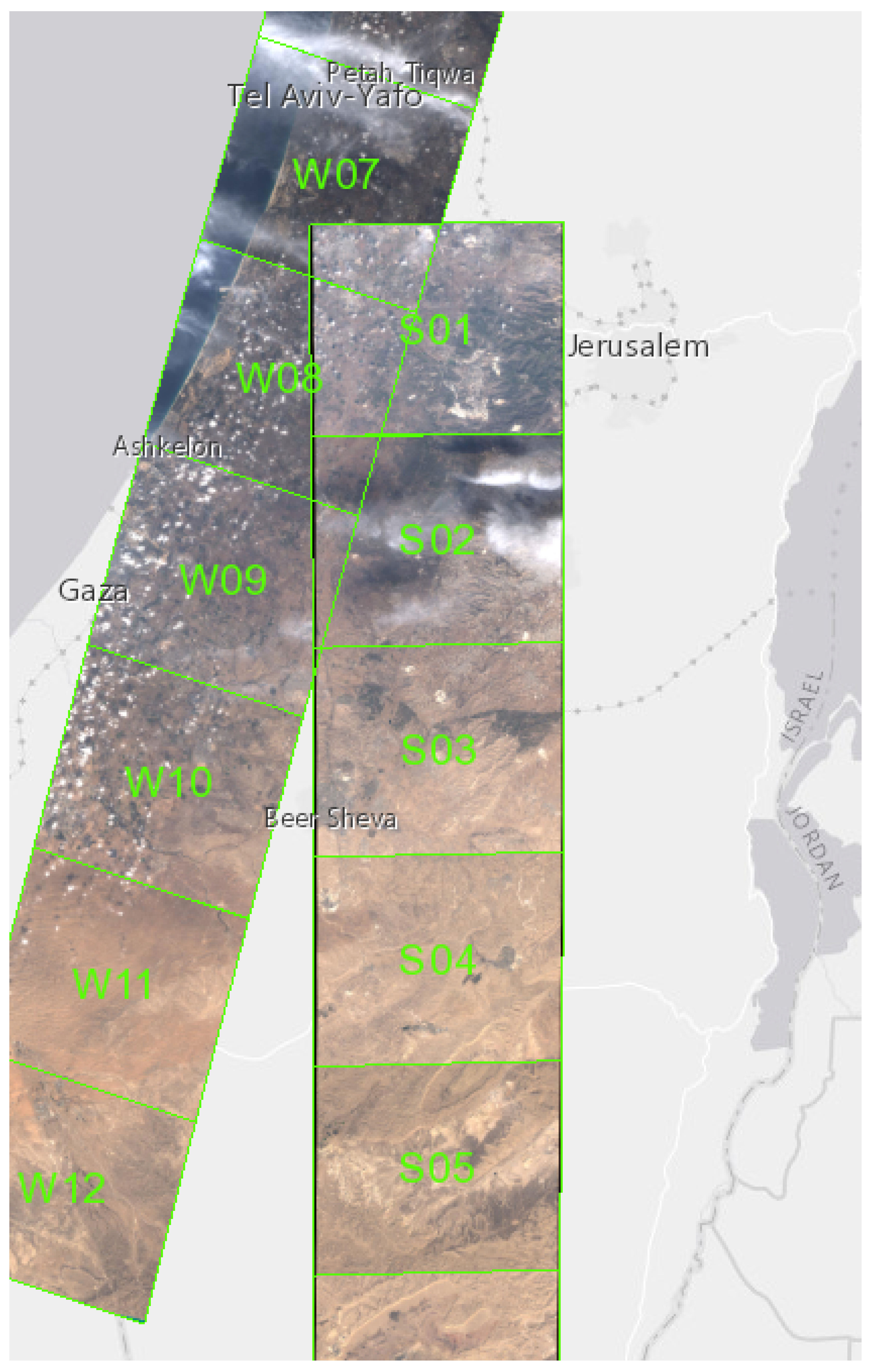
Figure 1. VEN μ S tile strips over Israel.
Remotesensing 14 05210 g001
Figure 2. Overview of chosen VEN μ S tiles: (a) Tile W07, covering water and urban areas; (b) Tile S01, covering agricultural and vegetated areas; (c) Tile S05, covering arid areas.
Remotesensing 14 05210 g002
Figure 3. Comparison of the MAJA cloud mask and manual label: (a) RGB representations of patches of VEN μ S tiles; (b) MAJA cloud mask (except for the thinnest clouds and cloud shadows); (c) manually labelled cloud mask.
Remotesensing 14 05210 g003
Figure 4. Comparison of manual binary and multi-class cloud masks: (a) RGB representations of patches of VEN μ S tiles; (b) binary mask; (c) multi-class mask, thick clouds (in grey) and thin clouds (in white).
Remotesensing 14 05210 g004
Figure 5. The workflow of the study.
Remotesensing 14 05210 g005
Figure 6. Overview of the commonly employed architectures for image segmentation in the field of remote sensing. Of the four most common encoder–decoder architectures, three were implemented: U-Net, SegNet, and DeepLab. Source: [42].
Remotesensing 14 05210 g006
Figure 7. An encoder–decoder CNN architecture with κ layers and skip connections; q l refers to the number of channels, m l denotes each channel dimension, and d l depicts the total dimension of the feature at the l-th layer. Source: [43].
Remotesensing 14 05210 g007
Figure 8. U-Net architecture. The channel number of feature maps is indicated on top of the boxes and the feature map size at the lower left/lower right edge of the image. In the experiment, it was enhanced by optional dropout layers following the CNN layers and by working with different feature map sizes, with the input being 1024 × 1024 pixels and convolutions used to preserve the shape. Source: [47].
Remotesensing 14 05210 g008
Figure 9. SegNet architecture. Source: [48].
Remotesensing 14 05210 g009
Figure 10. DeepLabv3+ architecture. Source: [57].
Remotesensing 14 05210 g010
Figure 11. Binary detection of clouds on a patch of an S01 VEN μ S tile from various architecture settings: (a) RGB representation of a patch of an S01 VEN μ S tile; (b) ground-truth mask; (c) U-Net—Dropout 0 %; (d) U-Net—Dropout 50%; (e) SegNet—Dropout 0%; (f) SegNet—Dropout 50%; (g) DeeplabV3+ with ResNet-50—Dropout 0%; (h) DeeplabV3+ with ResNet-50—Dropout 50%; (i) DeeplabV3+ with ResNet-101—Dropout 0%; (j) DeeplabV3+ with ResNet-101—Dropout 50%; (k) DeeplabV3+ with ResNet-152—Dropout 0%; (l) DeeplabV3+ with ResNet-152—Dropout 50%.
Remotesensing 14 05210 g011
Figure 12. Binary detection of clouds on a patch of an S05 VEN μ S tile from various architecture settings: (a) RGB representation of a patch of an S05 VEN μ S tile; (b) ground-truth mask; (c) U-Net—Dropout 0 %; (d) U-Net—Dropout 50%; (e) SegNet—Dropout 0%; (f) SegNet—Dropout 50%; (g) DeeplabV3+ with ResNet-50—Dropout 0%; (h) DeeplabV3+ with ResNet-50—Dropout 50%; (i) DeeplabV3+ with ResNet-101—Dropout 0%; (j) DeeplabV3+ with ResNet-101—Dropout 50%; (k) DeeplabV3+ with ResNet-152—Dropout 0%; (l) DeeplabV3+ with ResNet-152—Dropout 50%.
Remotesensing 14 05210 g012
Figure 13. Binary detection of clouds on a patch of an S05 VEN μ S tile with various inputs using U-Net—Dropout 0%. (a) RGB representation of a patch of an S05 VEN μ S tile; (b) ground-truth mask; (c) after a training using full-band input; (d) using only RGB; (e) using RGB enhanced with NDVI; (f) using augmented full-band input; (g) using only augmented RGB; (h) using augmented RGB enhanced with NDVI.
Remotesensing 14 05210 g013
Figure 14. Multi-class detection of clouds on a patch of an S05 Ven μ s tile with various inputs using U-Net—Dropout 0%. White represents thin clouds, grey represents thick clouds. (a) RGB representation of a patch of an S05 VEN μ S tile; (b) ground-truth mask; (c) after a training using full-band input; (d) using only RGB; (e) using RGB enhanced with NDVI; (f) using augmented full-band input; (g) using only augmented RGB; (h) using augmented RGB enhanced with NDVI.
Remotesensing 14 05210 g014
Figure 15. Comparison of the MAJA cloud mask and results from the binary detection of U-Net without dropout layers trained on the full-band dataset. A patch of S01 tile covering an urban area.
Remotesensing 14 05210 g015
Figure 16. Comparison of the MAJA cloud mask and results from the binary detection of U-Net without dropout layers trained on the full-band dataset. A patch of S05 tile covering an arid area.
Remotesensing 14 05210 g016
Table 1. VEN μ S spectral bands and their primary applications. Source: [38].
BandCentral Wavelength [nm]Bandwidth [nm]Main Application
Band 1423.940Atmospheric correction, water
Band 2446.940Aerosols, clouds
Band 3491.940Atmospheric correction, water
Band 4555.040Land
Band 5619.740Vegetation indices
Band 6619.740DEM, image quality
Band 7666.230Red edge
Band 8702.024Red edge
Band 9741.116Red edge
Band 10782.216Red edge
Band 11861.140Vegetation indices
Band 12908.720Water vapour
Table 2. Dice loss values over the validation dataset for different architectures and settings on the multi-class dataset. For rows: dN% stands for dropout, N specifies the dropout ratio, and rnN specifies the ResNet version used as a backbone model for DeepLabV3+. For columns: fb stands for the dataset utilizing the full-band images, rgb stands for the dataset utilizing only the red, green, and blue bands, rgb_ndvi represents rgb enhanced by the NDVI, and _a represents the augmented version of the dataset.
Architecturefbfb_argbrgb_argb_ndvirgb_ndvi_a
U-Net_d000.3300.3680.3840.4340.3480.340
U-Net_d500.3530.3620.4150.3800.4670.359
SegNet_d000.3830.4010.4060.4030.3730.372
SegNet_d500.4390.4220.4310.4970.4940.398
DeepLabV3+_rn50_d000.3780.4230.4310.4440.4350.506
DeepLabV3+_rn50_d500.4100.4290.4050.4450.3560.452
DeepLabV3+_rn101_d000.4230.4200.3750.3770.3860.349
DeepLabV3+_rn101_d500.4260.4520.4200.4060.3680.484
DeepLabV3+_rn152_d000.4110.3960.3800.3990.3530.356
DeepLabV3+_rn152_d500.4120.4360.4150.4040.3900.424
Table 3. Binary cross entropy loss values over the validation dataset for different architectures and settings on the binary dataset. For rows: dN% stands for dropout, N specifies the dropout ratio, and rnN specifies the ResNet version used as a backbone model for DeepLabV3+. For columns: fb stands for the dataset utilizing the full-band images, rgb stands for the dataset utilizing only the red, green, and blue bands, rgb_ndvi represents rgb enhanced by the NDVI, and _a represents the augmented version of the dataset.
Architecturefbfb_argbrgb_argb_ndvirgb_ndvi_a
U-Net_d000.0620.0900.0900.1000.0580.049
U-Net_d500.0690.0970.0890.0910.0910.114
SegNet_d000.1150.0940.1190.1070.0860.097
SegNet_d500.2680.1890.2390.1390.1140.141
DeepLabV3+_rn50_d000.1160.1810.0940.1070.1010.068
DeepLabV3+_rn50_d500.1370.1180.1110.1350.1180.125
DeepLabV3+_rn101_d000.0950.0750.1370.0650.2380.063
DeepLabV3+_rn101_d500.0970.1410.1110.1070.1530.122
DeepLabV3+_rn152_d000.1510.1710.1450.1590.1550.153
DeepLabV3+_rn152_d500.1800.1890.1920.1860.2220.226
Publisher’s Note: MDPI stays neutral with regard to jurisdictional claims in published maps and institutional affiliations.