
MSNet: Multifunctional Feature-Sharing Network for Land-Cover Segmentation


Abstract
1. Introduction
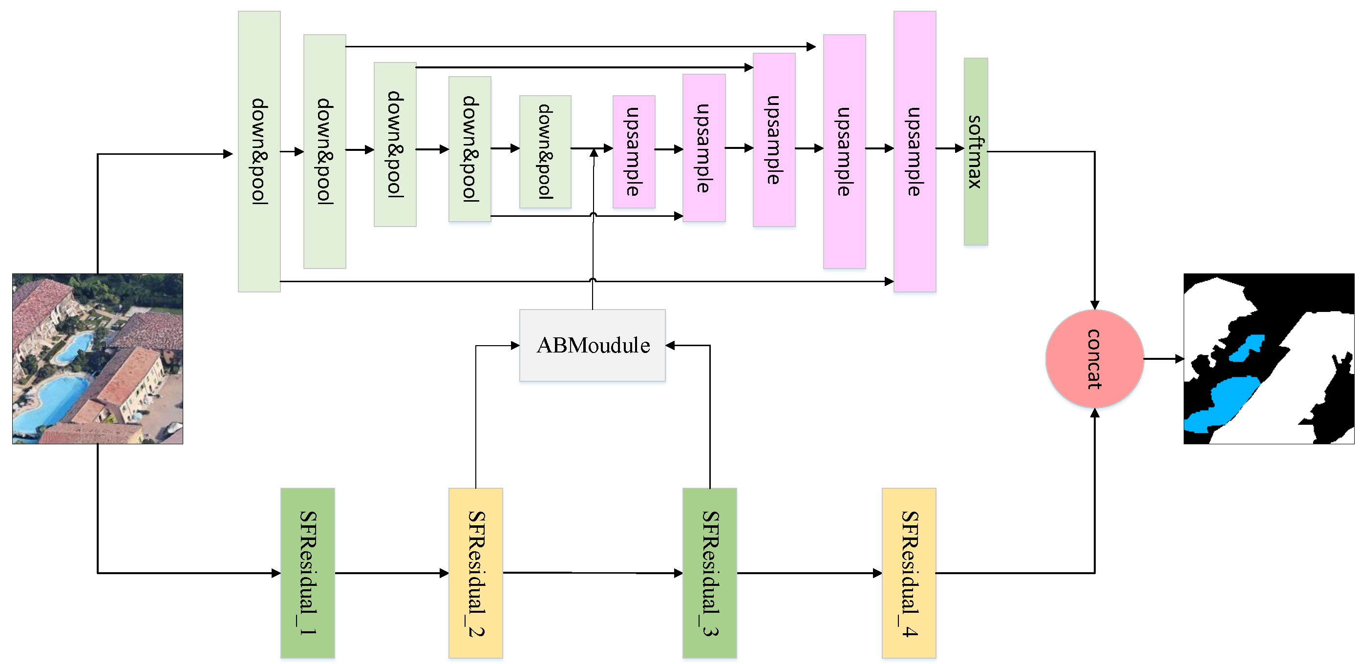
- One branch is a linear index upsampling branch with different levels. There is no need to learn upsampling. A trainable convolution kernel is used for convolution operations to acquire a complex feature map, which not only limits the amounts of calculations, but also ensures the integrity of high-frequency information.
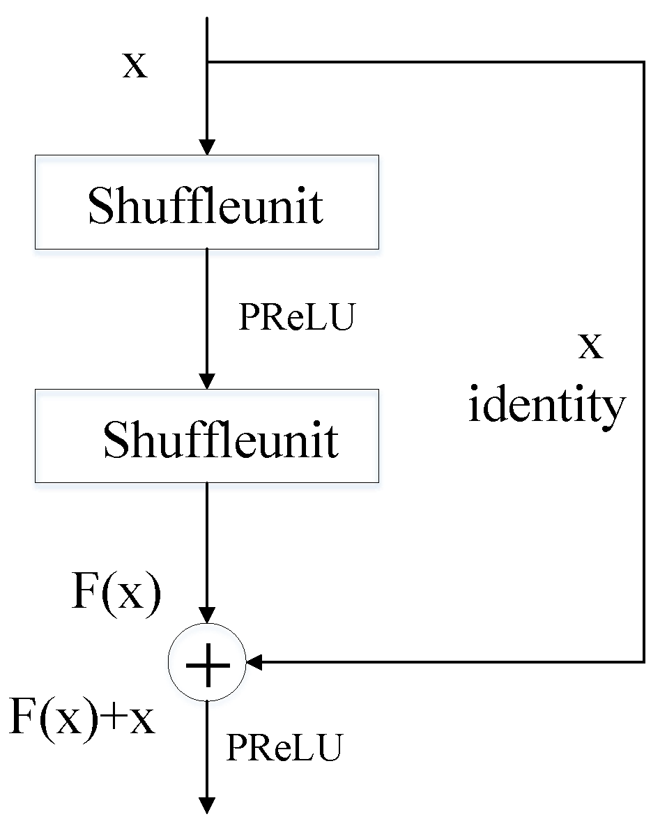
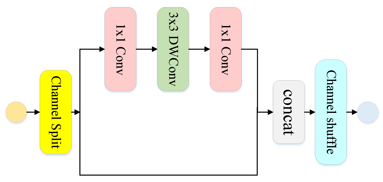
- The other branch combines a shuffle unit with a skip connection. Channel rearrangement makes the extraction of information more well distributed, and the residual structure ensures the accuracy of deep semantic information extraction. This branch extracts key features and pays attention to the dependencies between contexts by using the logical relationships [25] between information within a class and between classes.
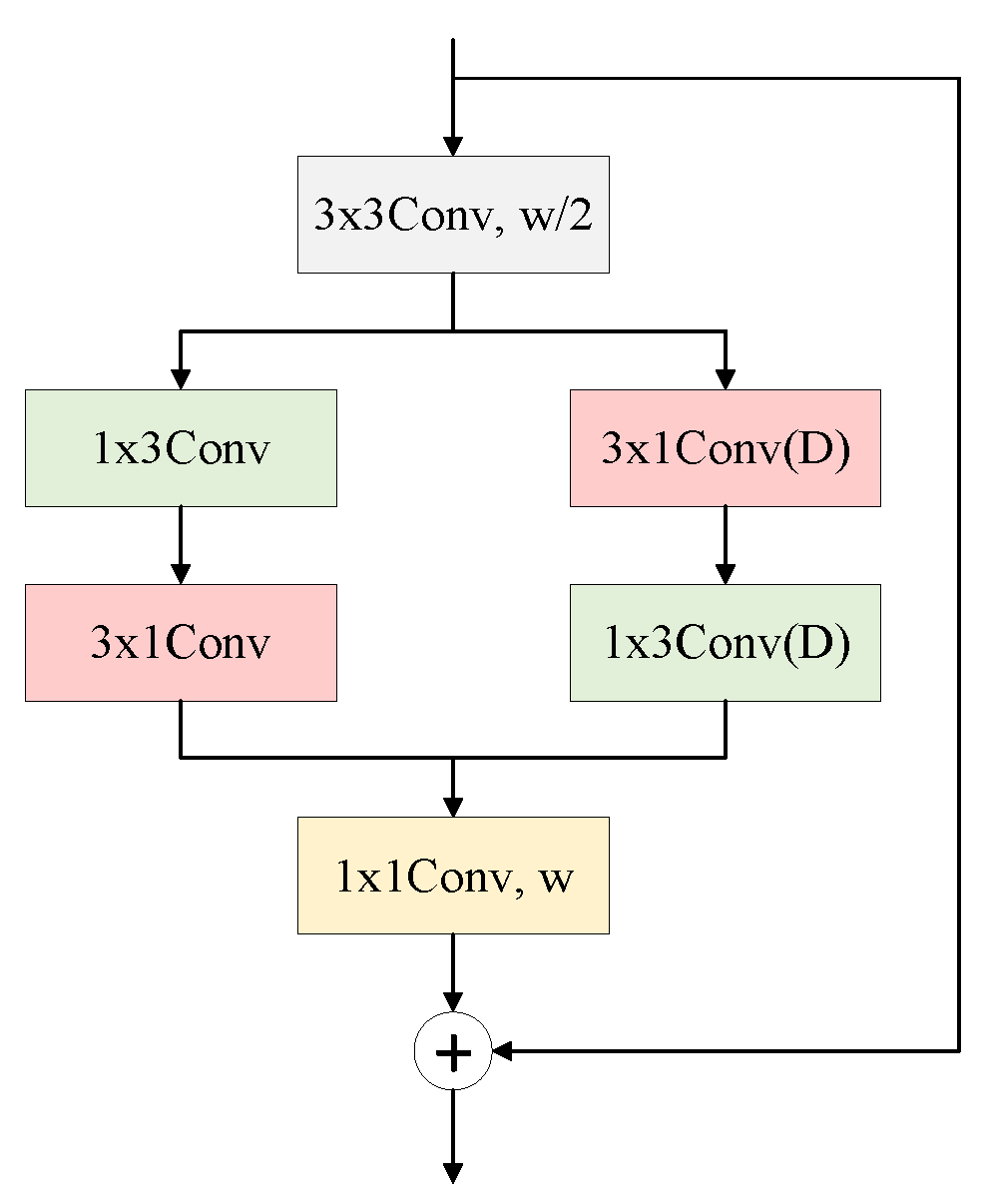
- After processing of the two SFR modules, the EFAModule is introduced to extract logical features and reply high-resolution detailed information, and good results in the learning of detailed information and edge information of a feature map were achieved.
2. Land-Cover Segmentation Methodology
2.1. Network Architecture
2.2. SFResidual
2.3. LIU Branch
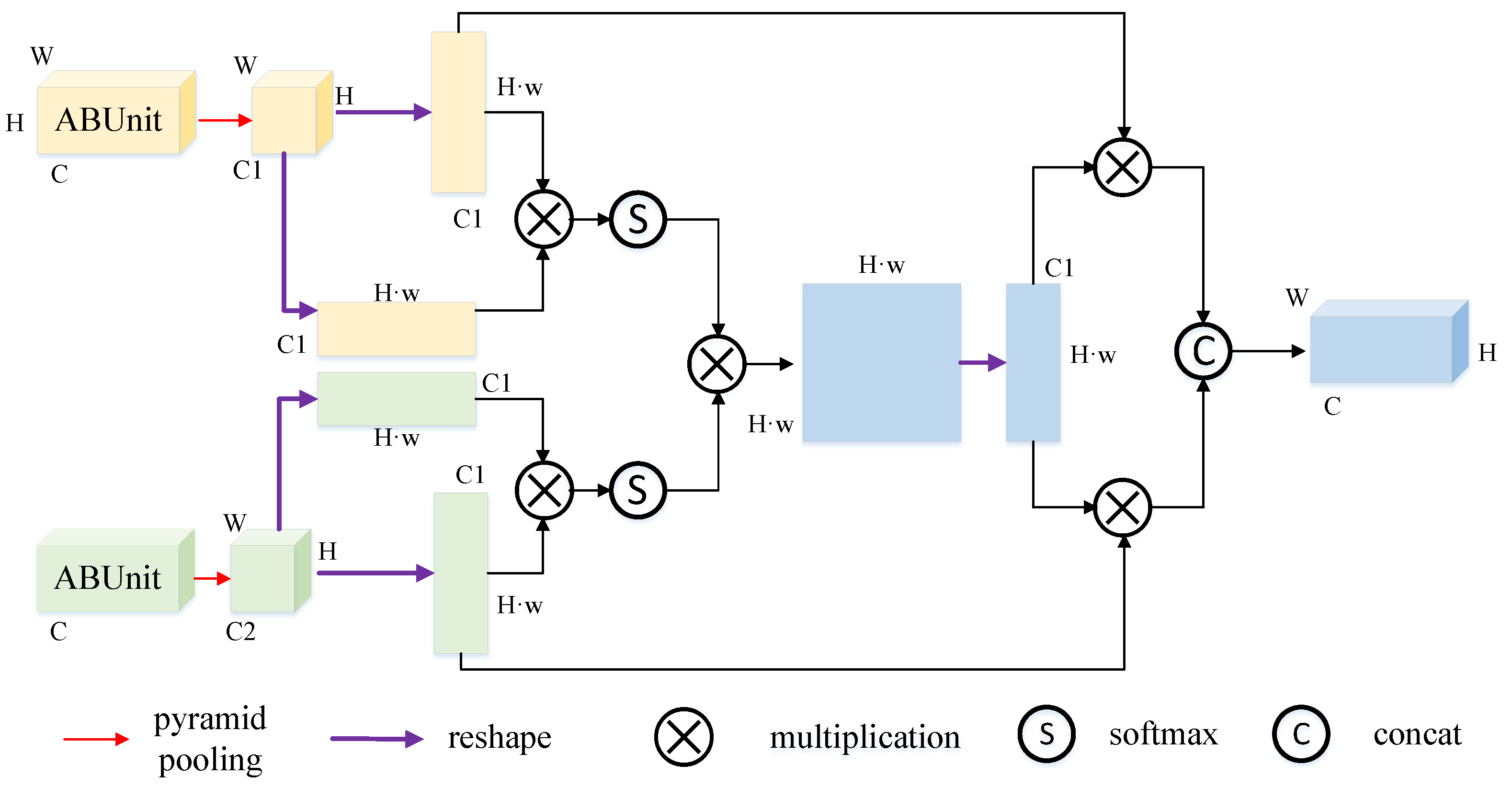
2.4. EFAModule
3. Land-Cover Segmentation Experiment
3.1. Dataset
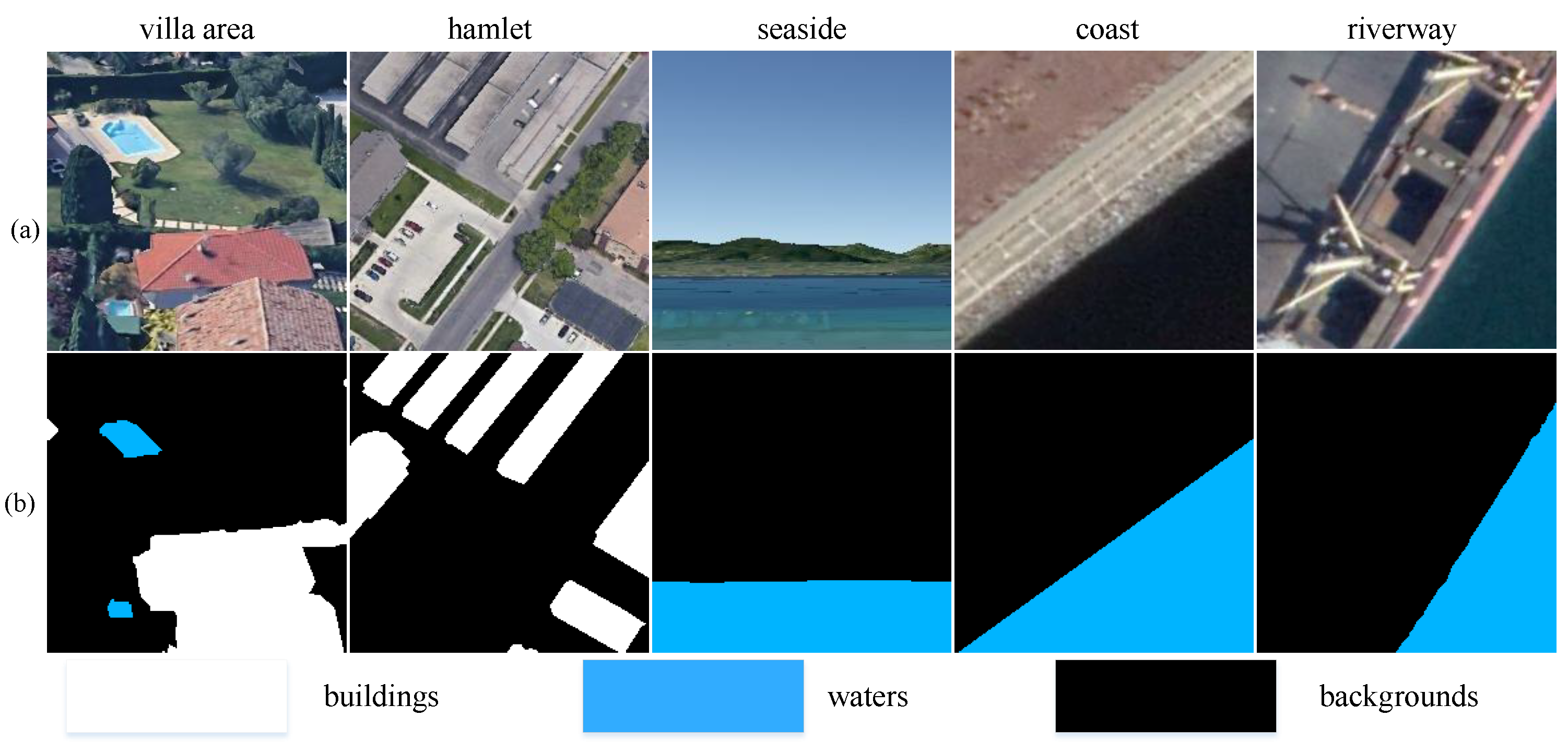
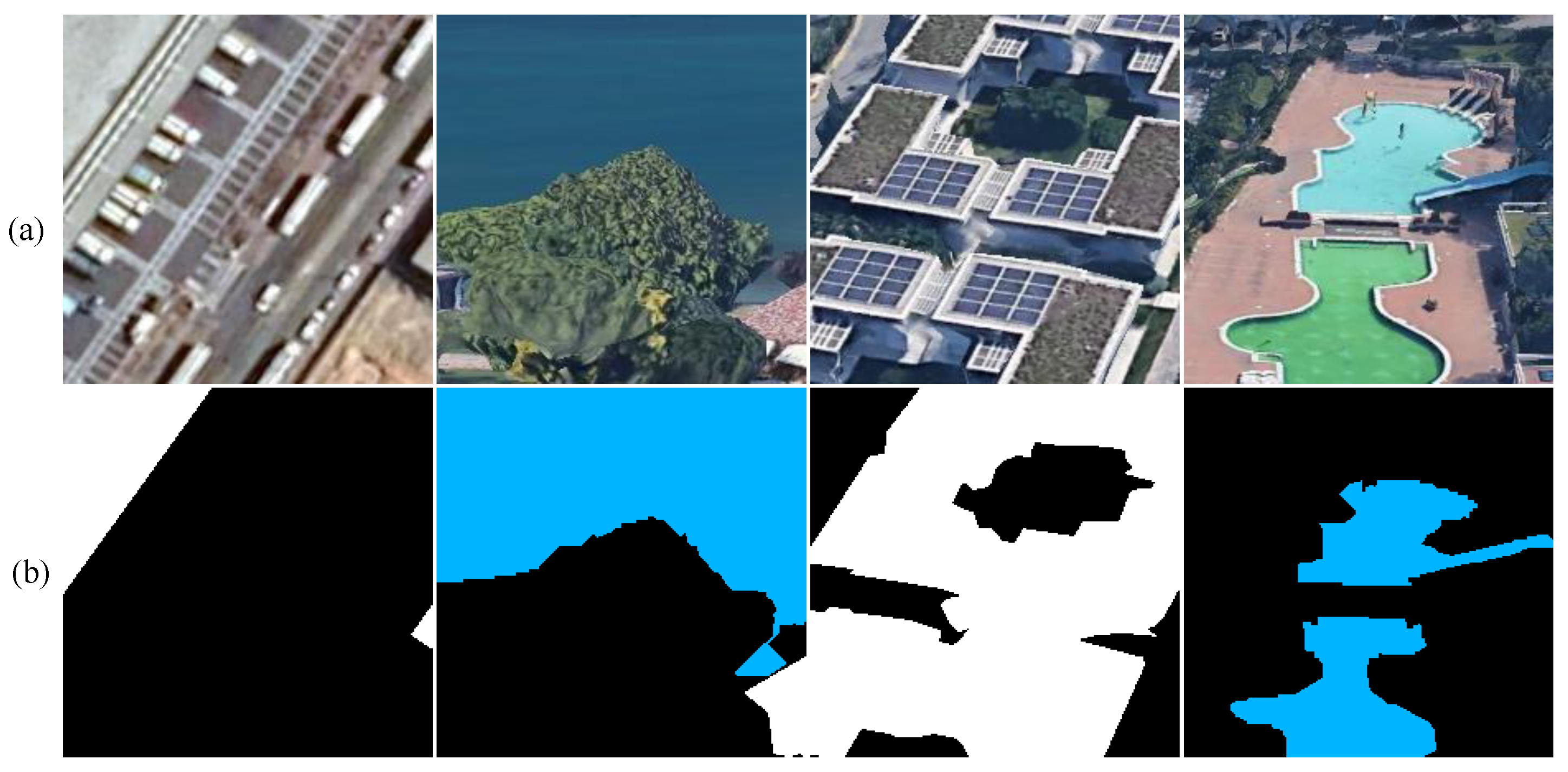
3.1.1. Land-Cover Dataset
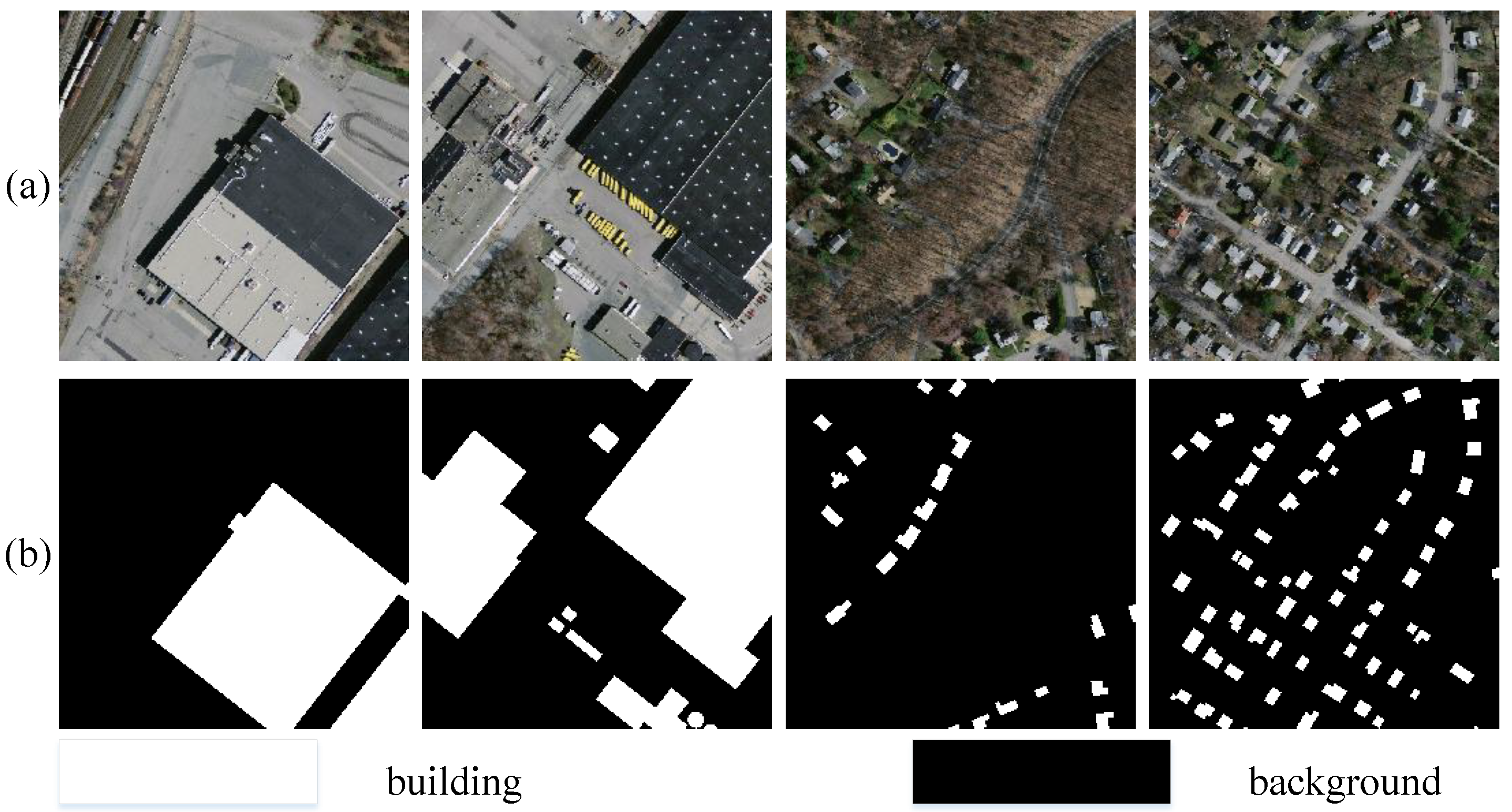
3.1.2. Public Dataset
3.1.3. Four-Class Public Dataset
3.2. Evaluation Index
3.3. Supplementary Experimental Procedures
3.4. Analysis of the Results
4. Conclusions
Author Contributions
Funding
Institutional Review Board Statement
Informed Consent Statement
Data Availability Statement
Conflicts of Interest
References
- Lu, C.; Xia, M.; Lin, H. Multi-scale strip pooling feature aggregation network for cloud and cloud shadow segmentation. Neural Comput. Appl. 2022, 34, 6149–6162. [Google Scholar] [CrossRef]
- Song, L.; Xia, M.; Jin, J.; Qian, M.; Zhang, Y. SUACDNet: Attentional change detection network based on siamese U-shaped structure. Int. J. Appl. Earth Obs. Geoinf. 2021, 105, 102597. [Google Scholar] [CrossRef]
- Wulder, M.A.; Masek, J.G.; Cohen, W.B.; Loveland, T.R.; Woodcock, C.E. Opening the archive: How free data has enabled the science and monitoring promise of Landsat. Remote Sens. Environ. 2012, 122, 2–10. [Google Scholar] [CrossRef]
- Bak, C.; Kocak, A.; Erdem, E.; Erdem, A. Spatio-temporal saliency networks for dynamic saliency prediction. IEEE Trans. Multimed. 2017, 20, 1688–1698. [Google Scholar] [CrossRef]
- Noble, W.S. What is a support vector machine? Nat. Biotechnol. 2006, 24, 1565–1567. [Google Scholar] [CrossRef] [PubMed]
- Xia, M.; Qu, Y.; Lin, H. PADANet: Parallel asymmetric double attention network for clouds and its shadow detection. J. Appl. Remote Sens. 2021, 15, 046512. [Google Scholar] [CrossRef]
- Potapov, P.V.; Turubanova, S.; Tyukavina, A.; Krylov, A.; McCarty, J.; Radeloff, V.; Hansen, M. Eastern Europe’s forest cover dynamics from 1985 to 2012 quantified from the full Landsat archive. Remote Sens. Environ. 2015, 159, 28–43. [Google Scholar] [CrossRef]
- Geller, G.N.; Halpin, P.N.; Helmuth, B.; Hestir, E.L.; Skidmore, A.; Abrams, M.J.; Aguirre, N.; Blair, M.; Botha, E.; Colloff, M.; et al. Remote sensing for biodiversity. In The GEO Handbook on Biodiversity Observation Networks; Springer: Cham, Switzerland, 2017; pp. 187–210. [Google Scholar]
- Gao, J.; Weng, L.; Xia, M.; Lin, H. MLNet: Multichannel feature fusion lozenge network for land segmentation. J. Appl. Remote Sens. 2022, 16, 016513. [Google Scholar] [CrossRef]
- Qu, Y.; Xia, M.; Zhang, Y. Strip pooling channel spatial attention network for the segmentation of cloud and cloud shadow. Comput. Geosci. 2021, 157, 104940. [Google Scholar] [CrossRef]
- Lu, C.; Xia, M.; Qian, M.; Chen, B. Dual-Branch Network for Cloud and Cloud Shadow Segmentation. IEEE Trans. Geosci. Remote Sens. 2022, 60, 5410012. [Google Scholar] [CrossRef]
- Chen, B.; Xia, M.; Qian, M.; Huang, J. MANet: A multi-level aggregation network for semantic segmentation of high-resolution remote sensing images. Int. J. Remote. Sens. 2022. [Google Scholar] [CrossRef]
- Wang, Z.; Xia, M.; Lu, M.; Pan, L.; Liu, J. Parameter Identification in Power Transmission Systems Based on Graph Convolution Network. IEEE Trans. Power Deliv. 2022, 37, 3155–3163. [Google Scholar] [CrossRef]
- Shokat, S.; Riaz, R.; Rizvi, S.S.; Abbasi, A.M.; Abbasi, A.A.; Kwon, S.J. Deep learning scheme for character prediction with position-free touch screen-based Braille input method. Hum.-Centric Comput. Inf. Sci. 2020, 10, 41. [Google Scholar] [CrossRef]
- Huang, H.; Lin, L.; Tong, R.; Hu, H.; Zhang, Q.; Iwamoto, Y.; Han, X.; Chen, Y.W.; Wu, J. Unet 3+: A full-scale connected unet for medical image segmentation. In Proceedings of the ICASSP 2020-2020 IEEE International Conference on Acoustics, Speech and Signal Processing (ICASSP), IEEE, Barcelona, Spain, 4–8 May 2020; pp. 1055–1059. [Google Scholar]
- Zhao, H.; Shi, J.; Qi, X.; Wang, X.; Jia, J. Pyramid scene parsing network. In Proceedings of the Proceedings of the IEEE Conference on Computer Vision and Pattern Recognition, Honolulu, HI, USA, 21–25 July 2017; pp. 2881–2890. [Google Scholar]
- Zhou, J.; Hao, M.; Zhang, D.; Zou, P.; Zhang, W. Fusion PSPnet image segmentation based method for multi-focus image fusion. IEEE Photonics J. 2019, 11, 6501412. [Google Scholar] [CrossRef]
- Chollet, F. Xception: Deep learning with depthwise separable convolutions. In Proceedings of the Proceedings of the IEEE Conference on Computer Vision and Pattern Recognition, Honolulu, HI, USA, 21–25 July 2017; pp. 1251–1258. [Google Scholar]
- Miao, S.; Xia, M.; Qian, M.; Zhang, Y.; Liu, J.; Lin, H. Cloud/shadow segmentation based on multi-level feature enhanced network for remote sensing imagery. Int. J. Remote. Sens. 2022. [Google Scholar] [CrossRef]
- Zhang, X.; Zhou, X.; Lin, M.; Sun, J. Shufflenet: An extremely efficient convolutional neural network for mobile devices. In Proceedings of the Proceedings of the IEEE Conference on Computer Vision and Pattern Recognition, Salt Lake City, UT, USA, 18–21 June 2018; pp. 6848–6856. [Google Scholar]
- Qin, X.; Wang, Z.; Bai, Y.; Xie, X.; Jia, H. FFA-Net: Feature fusion attention network for single image dehazing. In Proceedings of the AAAI Conference on Artificial Intelligence, New York, NY, USA, 7 February 2020; Volume 34, pp. 11908–11915. [Google Scholar]
- Hao, S.; Zhou, Y.; Zhang, Y.; Guo, Y. Contextual attention refinement network for real-time semantic segmentation. IEEE Access 2020, 8, 55230–55240. [Google Scholar] [CrossRef]
- O Oh, J.; Chang, H.J.; Choi, S.I. Self-Attention With Convolution and Deconvolution for Efficient Eye Gaze Estimation From a Full Face Image. In Proceedings of the IEEE/CVF Conference on Computer Vision and Pattern Recognition, New Orleans, LA, USA, 19–20 June 2022; pp. 4992–5000. [Google Scholar]
- Xia, M.; Wang, Z.; Lu, M.; Pan, L. MFAGCN: A new framework for identifying power grid branch parameters. Electr. Power Syst. Res. 2022, 207, 107855. [Google Scholar] [CrossRef]
- Khatami, R.; Mountrakis, G.; Stehman, S.V. A meta-analysis of remote sensing research on supervised pixel-based land-cover image classification processes: General guidelines for practitioners and future research. Remote Sens. Environ. 2016, 177, 89–100. [Google Scholar] [CrossRef]
- Huang, J.; Weng, L.; Chen, B.; Xia, M. DFFAN: Dual function feature aggregation network for semantic segmentation of land cover. ISPRS Int. J. Geo-Inf. 2021, 10, 125. [Google Scholar] [CrossRef]
- Zhao, J.; Du, B.; Sun, L.; Zhuang, F.; Lv, W.; Xiong, H. Multiple relational attention network for multi-task learning. In Proceedings of the 25th ACM SIGKDD International Conference on Knowledge Discovery & Data Mining, Anchorage, AK, USA, 4–8 August 2019; pp. 1123–1131. [Google Scholar]
- Cheng, X.; Zhang, Y.; Chen, Y.; Wu, Y.; Yue, Y. Pest identification via deep residual learning in complex background. Comput. Electron. Agric. 2017, 141, 351–356. [Google Scholar] [CrossRef]
- Ren, S.; Sun, J.; He, K.; Zhang, X. Deep residual learning for image recognition. In Proceedings of the CVPR, Vegas, NV, USA, 27–30 June 2016; Volume 2, p. 4. [Google Scholar]
- Liu, J.; He, J.; Qiao, Y.; Ren, J.S.; Li, H. Learning to predict context-adaptive convolution for semantic segmentation. In Proceedings of the European Conference on Computer Vision; Springer: Berlin/Heidelberg, Germany, 2020; pp. 769–786. [Google Scholar]
- Sengupta, A.; Ye, Y.; Wang, R.; Liu, C.; Roy, K. Going deeper in spiking neural networks: VGG and residual architectures. Front. Neurosci. 2019, 13, 95. [Google Scholar] [CrossRef] [PubMed]
- Pang, K.; Weng, L.; Zhang, Y.; Liu, J.; Lin, H.; Xia, M. SGBNet: An Ultra Light-weight Network for Real-time Semantic Segmentation of Land Cover. Int. J. Remote. Sens. 2022. [Google Scholar] [CrossRef]
- Yu, C.; Wang, J.; Peng, C.; Gao, C.; Yu, G.; Sang, N. Bisenet: Bilateral segmentation network for real-time semantic segmentation. In Proceedings of the European Conference on Computer Vision (ECCV), Munich, Germany, 13 September 2018; pp. 325–341. [Google Scholar]
- Li, X.; Li, X.; Zhang, L.; Cheng, G.; Shi, J.; Lin, Z.; Tan, S.; Tong, Y. Improving Semantic Segmentation via Decoupled Body and Edge Supervision Supplementary. In Proceedings of the ECCV, Glasgow, UK, 23–28 August 2020; Volume 17, pp. 435–452. [Google Scholar]
- Mehta, S.; Paunwala, C.; Vaidya, B. CNN based traffic sign classification using adam optimizer. In Proceedings of the 2019 International Conference on Intelligent Computing and Control Systems (ICCS), IEEE, Madurai, India, 15–17 May 2019; pp. 1293–1298. [Google Scholar]
- Hu, H.; Ji, D.; Gan, W.; Bai, S.; Wu, W.; Yan, J. Class-wise dynamic graph convolution for semantic segmentation. In Proceedings of the European Conference on Computer Vision; Springer: Berlin/Heidelberg, Germany, 2020; pp. 1–17. [Google Scholar]
- Boguszewski, A.; Batorski, D.; Ziemba-Jankowska, N.; Dziedzic, T.; Zambrzycka, A. LandCover. ai: Dataset for automatic mapping of buildings, woodlands, water and roads from aerial imagery. In Proceedings of the IEEE/CVF Conference on Computer Vision and Pattern Recognition, Long Beach, CA, USA, 19–25 June 2021; pp. 1102–1110. [Google Scholar]
- Marugg, J.D.; Gonzalez, C.F.; Kunka, B.S.; Ledeboer, A.M.; Pucci, M.J.; Toonen, M.Y.; Walker, S.A.; Zoetmulder, L.C.; Vandenbergh, P.A. Cloning, expression, and nucleotide sequence of genes involved in production of pediocin PA-1, and bacteriocin from Pediococcus acidilactici PAC1.0. Appl. Environ. Microbiol. 1992, 58, 2360–2367. [Google Scholar] [CrossRef] [PubMed]
- Xia, M.; Zhang, X.; Weng, L.; Xu, Y. Multi-stage feature constraints learning for age estimation. IEEE Trans. Inf. Forensics Secur. 2020, 15, 2417–2428. [Google Scholar] [CrossRef]
- Li, S.; Zhao, X.; Zhou, G. Automatic pixel-level multiple damage detection of concrete structure using fully convolutional network. Comput.-Aided Civ. Infrastruct. Eng. 2019, 34, 616–634. [Google Scholar] [CrossRef]
- Seifi, S.; Tuytelaars, T. Attend and segment: Attention guided active semantic segmentation. In Proceedings of the European Conference on Computer Vision; Springer: Berlin/Heidelberg, Germany, 2020; pp. 305–321. [Google Scholar]
- Chen, Y.; Li, Y.; Wang, J.; Chen, W.; Zhang, X. Remote sensing image ship detection under complex sea conditions based on deep semantic segmentation. Remote Sens. 2020, 12, 625. [Google Scholar] [CrossRef]
- Bock, S.; Goppold, J.; Weiß, M. An improvement of the convergence proof of the ADAM-Optimizer. arXiv 2018, arXiv:1804.10587. [Google Scholar]
- Ho, Y.; Wookey, S. The real-world-weight cross-entropy loss function: Modeling the costs of mislabeling. IEEE Access 2019, 8, 4806–4813. [Google Scholar] [CrossRef]
- Gordon-Rodriguez, E.; Loaiza-Ganem, G.; Pleiss, G.; Cunningham, J.P. Uses and abuses of the cross-entropy loss: Case studies in modern deep learning. arXiv 2020, arXiv:2011.05231. [Google Scholar]
- Mehta, S.; Rastegari, M.; Caspi, A.; Shapiro, L.; Hajishirzi, H. Espnet: Efficient spatial pyramid of dilated convolutions for semantic segmentation. In Proceedings of the European Conference on Computer Vision (ECCV), Munich, Germany, 13 September 2018; pp. 552–568. [Google Scholar]
- Badrinarayanan, V.; Handa, A.; Cipolla, R. Segnet: A deep convolutional encoder-decoder architecture for robust semantic pixel-wise labelling. arXiv 2015, arXiv:1505.07293. [Google Scholar]
- Zhang, S.; Wu, G.; Costeira, J.P.; Moura, J.M. Fcn-rlstm: Deep spatio-temporal neural networks for vehicle counting in city cameras. In Proceedings of the IEEE International Conference on Computer Vision, Honolulu, HI, USA, 22–25 July 2017; pp. 3667–3676. [Google Scholar]
- Li, G.; Yun, I.; Kim, J.; Kim, J. Dabnet: Depth-wise asymmetric bottleneck for real-time semantic segmentation. arXiv 2019, arXiv:1907.11357. [Google Scholar]
- Mehta, S.; Rastegari, M.; Shapiro, L.; Hajishirzi, H. Espnetv2: A light-weight, power efficient, and general purpose convolutional neural network. In Proceedings of the IEEE/CVF Conference on Computer Vision and Pattern Recognition, Long Beach, CA, USA, 16–20 June 2019; pp. 9190–9200. [Google Scholar]
- Yuan, Y.; Chen, X.; Chen, X.; Wang, J. Segmentation transformer: Object-contextual representations for semantic segmentation. arXiv 2019, arXiv:1909.11065. [Google Scholar]
- Park, H.; Sjösund, L.L.; Yoo, Y.; Bang, J.; Kwak, N. Extremec3net: Extreme lightweight portrait segmentation networks using advanced c3-modules. arXiv 2019, arXiv:1908.03093. [Google Scholar]
- Paszke, A.; Chaurasia, A.; Kim, S.; Culurciello, E. Enet: A deep neural network architecture for real-time semantic segmentation. arXiv 2016, arXiv:1606.02147. [Google Scholar]
- Yang, J.; Fu, X.; Hu, Y.; Huang, Y.; Ding, X.; Paisley, J. PanNet: A deep network architecture for pan-sharpening. In Proceedings of the IEEE International Conference on Computer Vision, Honolulu, HI, USA, 22–25 July 2017; pp. 5449–5457. [Google Scholar]
- Yu, C.; Gao, C.; Wang, J.; Yu, G.; Shen, C.; Sang, N. Bisenet v2: Bilateral network with guided aggregation for real-time semantic segmentation. arXiv 2020, arXiv:2004.02147. [Google Scholar] [CrossRef]


| Branch 1 | Branch 2 | Middle Branch |
|---|---|---|
| 3 × 3 conv | shuffleNet ×2 +PReLU, 16 | 1 × 3 conv, 3 × 1 conv |
| maxpool | shuffleNet ×2 +PReLU, 28 | 3 × 1 conv, 1 × 3 conv |
| groups conv + point conv | shuffleNet ×2 +PReLU, 40 | EFAModule |
| deconv ×2 | shuffleNet ×2 +PReLU, 56 | |
| softmax |
| Method | PA (%) | MPA (%) | MIoU (%) | Flops (G) | Parameters (M) |
|---|---|---|---|---|---|
| SFR | 87.69 | 87.96 | 75.62 | 0.96 | 0.039 |
| EFA | 79.56 | 77.96 | 70.62 | 0.05 | 0.0001 |
| LIU | 88.75 | 88.51 | 79.59 | 134.27 | 73.34 |
| SFR + EFA | 88.48 | 87.27 | 76.65 | 1.01 | 0.039 |
| SFR + LIU | 88.09 | 88.56 | 78.13 | 20 | 17.5 |
| SFR + LIU + EFA | 89.84 | 89.62 | 81.33 | 21.86 | 18.7 |
| Method | PA (%) | MPA (%) | MIoU (%) | Parameters (M) | Flops (G) |
|---|---|---|---|---|---|
| UNet | 86.89 | 85.66 | 75.18 | 17.27 | 40 |
| SegNet [47] | 87.95 | 88.35 | 75.95 | 29.44 | 40.07 |
| FCN8s | 89.43 | 88.51 | 79.59 | 134.27 | 73.35 |
| FCN32s [48] | 89.75 | 88.35 | 79.37 | 134.29 | 73.34 |
| PSPNet [16] | 89.29 | 89.75 | 80.14 | 48.94 | 44.3 |
| DABNet [49] | 89.55 | 89.90 | 79.89 | 0.75 | 2.82 |
| EspNetV2 [50] | 89.46 | 89.59 | 79.95 | 1.24 | 0.66 |
| OcrNet [51] | 89.97 | 89.51 | 80.09 | 70.35 | 40.4 |
| ExtremeC3Net [52] | 88.69 | 88.05 | 78.04 | 0.04 | 1.27 |
| MSNet | 89.84 | 89.62 | 81.33 | 18.7 | 21.86 |
| Method | MIoU(%) | Parameters (M) | Flops (G) |
|---|---|---|---|
| UNet | 69.5 | 17.27 | 40 |
| SegNet | 72.17 | 29.44 | 40.07 |
| PSPNet | 77.08 | 48.94 | 44.3 |
| ENet [53] | 70.52 | 0.35 | 0.45 |
| DeeplabV3+Net | 75.28 | 91.77 | 64.42 |
| DABNet | 75.14 | 0.752 | 1.27 |
| Pan [54] | 74.48 | 23.65 | 1.27 |
| BiseNetV2 [55] | 74.63 | 3.62 | 3.2 |
| MSNet | 79.90 | 18.7 | 21.01 |
| Method | MIoU (%) | Parameters (M) | Flops (G) |
|---|---|---|---|
| UNet | 89.5 | 17.27 | 40 |
| SegNet | 95.17 | 29.44 | 40.07 |
| PSPNet | 97.08 | 48.94 | 44.3 |
| ENet [53] | 70.52 | 0.35 | 0.45 |
| DeeplabV3+Net | 97.28 | 91.77 | 64.42 |
| DABNet | 97.14 | 0.752 | 1.27 |
| Pan [54] | 97.48 | 23.65 | 1.27 |
| BiseNetV2 [55] | 97.93 | 3.62 | 3.2 |
| MSNet | 98.94 | 18.7 | 21.01 |
| Method | MIoU (%) | PA | MPA |
|---|---|---|---|
| UNet | 64.49 | 73.31 | 79.91 |
| SegNet | 68.67 | 85.09 | 87.14 |
| FCN32s | 77.65 | 89.54 | 89.32 |
| DeeplabV3+Net | 76.86 | 87.85 | 87.07 |
| DABNet | 73.33 | 86.46 | 87.39 |
| ExtremeC3Net | 71.75 | 85.99 | 85.11 |
| MSNet | 78.79 | 90.21 | 88.64 |
Publisher’s Note: MDPI stays neutral with regard to jurisdictional claims in published maps and institutional affiliations. |
© 2022 by the authors. Licensee MDPI, Basel, Switzerland. This article is an open access article distributed under the terms and conditions of the Creative Commons Attribution (CC BY) license (https://creativecommons.org/licenses/by/4.0/).
Share and Cite
Weng, L.; Gao, J.; Xia, M.; Lin, H. MSNet: Multifunctional Feature-Sharing Network for Land-Cover Segmentation. Remote Sens. 2022, 14, 5209. https://doi.org/10.3390/rs14205209
Weng L, Gao J, Xia M, Lin H. MSNet: Multifunctional Feature-Sharing Network for Land-Cover Segmentation. Remote Sensing. 2022; 14(20):5209. https://doi.org/10.3390/rs14205209
Chicago/Turabian StyleWeng, Liguo, Jiahong Gao, Min Xia, and Haifeng Lin. 2022. "MSNet: Multifunctional Feature-Sharing Network for Land-Cover Segmentation" Remote Sensing 14, no. 20: 5209. https://doi.org/10.3390/rs14205209
APA StyleWeng, L., Gao, J., Xia, M., & Lin, H. (2022). MSNet: Multifunctional Feature-Sharing Network for Land-Cover Segmentation. Remote Sensing, 14(20), 5209. https://doi.org/10.3390/rs14205209