Abstract
In this paper, we propose a partial ambiguity method of global navigation satellite system (GNSS) reliable positioning based on a robust estimation model to address the problems of the low reliability and availability of GNSS positioning in urban complex environments. First, the high-precision observations selected on the basis of the signal-to-noise ratio (SNR) were used to solve ambiguities. Then, the fixed ambiguities were used as constraints to solve the ambiguities of low-quality observations. The robust estimation method was used to reduce the impact of outliers for the ambiguity solutions. The robust estimation was also used to solve the position parameters to reduce the influence of the residual errors and uncorrected ambiguities for GNSS high-accuracy positioning. Static and dynamic data were used to evaluate the proposed algorithm. These experiments show that the proposed algorithm with the robust estimation can reduce the fixed time of ambiguity initialization, compared with the conventional algorithm without the robust estimation. The positioning accuracy and solution rate are similar regardless of whether the robust estimation is used in the GNSS unblocked environment. In blocked environments, the solution rate improves to more than 99%, and the three-dimensional (3D) position accuracy improves by more than 70% when the robust estimation is used. When the observation number of simulated small gross error accounts for 40.91% of total observations, the centimeter-level positioning accuracy can still be obtained via several robust estimation models. In the urban blocked environment, the IGG (Institute of Geodesy and Geophysics) III scheme has a better performance than other robust schemes discussed in this paper with regard to the positioning performance and computational efficiency.
1. Introduction
The global network completion of the Beidou Navigation Satellite System (BDS), along with the Global Positioning System (GPS) and Global Navigation Satellite System (GLONASS), ensures that there are enough satellites currently operating [1]. The geometric structure of a single system can be improved by a multi-satellite system, which ensures positioning accuracy and reliability [2]. Multisystem global navigation satellite system (GNSS) positioning is a research trend, and it has been widely applied in mobile mapping, intelligent driving, and smart agriculture [3,4].
A high-accuracy, continuous, and robust position reference is required for mapping of mobile mapping systems and intelligent driving. However, GNSS observations are susceptible to the influence of blocked environments, and gross errors inevitably occur in observations, resulting in biased estimations [5,6]. Currently, these processing methods of gross errors are outlier detection and robust estimation [7]. The original outlier detection theory was proposed in Baarda’s study, which makes a decision between the null hypothesis and alternative hypothesis [8]. The observation of outlier that was detected was excluded, and the remaining observations were used for parameter estimation. In general, outlier detection can better process the single gross error of observations, and the gross error cannot be effectively identified when there are multiple outliers in observations. The method of robust estimation is relatively insensitive to outliers, and it not only excludes doubtful observations but also restrains the impacts of those doubtful observations [9]. The robust estimation method is widely used for the gross error process, which improves the accuracy by reducing the weight of contaminated observations. The key to robust estimation is the equivalent weight function. To effectively reduce the influence of gross error for parameter estimation, Huber proposed the M-estimation theory [10]. Zhou [11] proposed an equivalent weight function named the IGG scheme. Yang et al. [12] proposed the IGGIII scheme that divided the equivalent weight function into three segments. To adjust the correlation of observations, Yang et al. [13] developed robust estimation based on a bifactor model, in which the equivalent weight matrix was symmetric and the original correlation coefficients of observations were unchanged. Wang et al. [14] used robust estimation with equivalent weight based on the Huber function to suppress the measurement model error. The Hampel function, Tukey function, and Danish function are also widely used to construct equivalent weight functions to resist the impacts of outliers [15,16]. To reduce the influence of outliers for GNSS high-accuracy positioning, robust estimation is widely used in GNSS positioning [17,18,19]. Wang et al. [20] used robust estimation to process GPS positioning, and experiments showed that the robust estimation method effectively reduced the impact of small gross errors. Wang et al. [21] also applied robust estimations to network real-time kinematic (NRTK) positioning, and these experiments showed that the robust estimation algorithm could improve the positioning accuracy of single-epoch NRTK. In blocked environments, satellite signals are susceptible to interference, and the performance of GNSS positioning can be improved significantly by the robust estimation method [22,23]. Crespillo et al. [24] used robust estimation for GNSS positioning to reduce the impact of multipath/non-line-of-sight signals, and these experiments showed that the maximum error can be reduced in urban environments. To reduce the influence of residual atmospheric errors, a robust estimation algorithm was used [25] to effectively improve the accuracy of long baseline GNSS RTK positioning. The correctly fixed ambiguity is the key to obtaining continuous high-precision positioning [26]. The robust estimation algorithm can effectively identify outliers, and the accuracy of the ambiguity solution can be improved [27]. In one study [28], the influence of non-line-of-sight errors was reduced by the robust estimation method, and the performance of the ambiguity resolution was improved in complex environments. The robust estimation can effectively reduce the impact of the gross error and small cycle slip of GNSS observations, and the fixed rate of ambiguity and positioning accuracy can be improved [29].
At present, a single model of robust estimation used for GNSS positioning is being studied, but there are few analyses on the performance of different robust estimations in urban environments. Therefore, we propose a robust algorithm of GNSS high-accuracy positioning based on carrier phase observations and analyze the positioning performance of different robust estimation models. This proposed strategy of GNSS positioning uses robust estimation for ambiguity resolution and position parameter estimation, which reduces the influence of outliers for position estimation in complex urban environments, and a continuous, reliable, and high-accuracy position reference can be provided for mapping of mobile mapping system and intelligent driving. The structure of this paper is as follows: Section 2 introduces our proposed robust algorithm of GNSS positioning. In Section 3, the collected static and kinematic data are used to analyze the performance of the proposed algorithm with different robust estimation models. Section 4 includes our summary and conclusions.
2. Methods
2.1. Observation Model
The double-difference method can eliminate or reduce most errors of GNSS observations, and it is widely used for high-accuracy GNSS positioning. The double-difference equations of the GNSS based on observations of the pseudo-range and carrier phase are as follows [30,31]:
where and represent satellite numbers, , , and represent the satellite frequency number, reference station, and mobile station, respectively, is the double-difference operator, represents the pseudo-range observation, represents the carrier-phase observation, is the geometric distance from the satellite to the receiver, is the wavelength of the frequency, is the integer ambiguity, represents the tropospheric delay, represents the ionospheric delay of the first frequency, is the conversion coefficient of ionospheric delay from the first frequency to frequency, is the frequency of the first waveband, represents other errors that are independent of the frequency, and and represent noises of the pseudo-range and carrier phase, respectively.
After linearization of Equations (1) and (2), the error equation can be obtained as follows:
where represents the residual, and are design matrices of the parameter estimations, represents the estimated position parameters, and represents the observation value.
The least squares method is used to solve Equation (3), and the floated ambiguities and the corresponding variance–covariance are obtained. In this paper, we used the LAMBDA algorithm to fix ambiguities. The ratio value and unit weight of the standard error were used to confirm ambiguity. To further improve the accuracy of the ambiguity solution, we propose a partial ambiguity method based on wide-lane (WL) guidance. First, the WL ambiguity of high-quality observations selected on the basis of the signal-to-noise ratio (SNR) is fixed, and then the fixed ambiguity is used as a constraint to solve the residual ambiguities [32]:
where is the fixed solution, and represents the floated solution.
The least squares method is used to solve Equation (4), and the strength of the equation is enhanced because of the constraint of the fixed ambiguities. The robust estimation is used in solving Equation (4) to reduce the influence of outliers for the ambiguity solution.
After the WL ambiguity is fixed, the basic ambiguity can be solved according to the relationship between the WL observation equation and the basic observation equation. The fixed WL ambiguity is brought into the WL observation equation of the carrier phase, and then the WL observation equation subtracts the basic observation to calculate basic ambiguity.
where is the float ambiguity of the basic observation equation, is the fixed WL ambiguity, is the WL observation of the carrier phase, and is the WL wavelength.
The float ambiguity calculated using Equation (5) can be rounded directly for a short baseline. After the basic ambiguity is fixed, it is substituted into Equation (3), and the observation equation based on the carrier phase is used to solve the position parameters:
where is the weight matrix.
The SNR can reflect the quality of observations. When the quality of observations is lower, the SNR is smaller. Therefore, the random model based on the SNR was used in this paper:
where is the SNR, represents the phase tracking bandwidth, and takes an empirical value in practical applications [33].
To resist outliers of the GNSS observations, the robust estimation is used to improve the accuracy of the parameter estimation:
where is the equivalent weight, and is the weight factor of the robust estimation.
In urban blocked environments, different weight factors are selected, and the robust performance of GNSS positioning is different. Next, several equivalent weight functions are discussed.
2.2. Equivalent Weight Function
2.2.1. Andrews Function
The Andrews function contains the weight reduction segment and elimination segment, and its weight factor can be expressed as follows [34]:
where is the standardized residual, is the standard deviation, and is a constant (taken as 1.339 in this paper).
2.2.2. Danish Function
The Danish function includes a normal segment and weight reduction segment, and its weight factor can be expressed as follows [7]:
where represents the exponential function, and is a constant (taken as 1.5 in this paper).
2.2.3. Hampel Function
The Hampel function includes the normal segment, weight reduction segment, and eliminated segment, and its weight factor can be expressed as follows [16]:
where , , and are the modulation coefficients, which are 1.7, 3.4, and 8.5, respectively, in this paper.
2.2.4. Huber Function
The Huber function consists of a normal segment and weight reduction segment, and its weight factor can be expressed as follows [35,36]:
where is a constant (taken as 2.0 in this paper).
2.2.5. IGGIII Function
The IGGIII function contains the normal segment, weight reduction segment, and eliminated segment, and its weight factor can be expressed as follows [13]:
where represents the quantile parameter, and represents the elimination points. In this paper, and were taken as 1.2 and 2.8, respectively.
2.2.6. Tukey Function
The Tukey function contains the weight reduction segment and elimination segment, and its weight factor can be expressed as follows [37]:
where is the regression factor (taken as 4.685 in this paper).
Figure 1 shows the weight factor of different robust estimation functions described in Section 2.2.1 to Section 2.2.6, with ranging from −10 m to 10 m. In Figure 1, the curves of weight factor of Andrews function and Tukey function are similar. The parameters estimated using Equations (9) and (10) are either decreased in weight as is or the outliers are discarded, and the weight factor of observation is one only when is equal to zero, which almost reduces the weight of observations used for parameters estimation. The weight value calculated by the Danish function is either left as is or decreased, and the weight factor gradually approaches zero as increases. The weight factor calculated by the Hampel function includes four segments. The weight factor is one when the is less than or equal to 1.7 m, the weight factor is zero when is greater than 8.5 m, and the weight factor is decreased when is greater than 1.7 m but less than or equal to 8.5. The weight value calculated by the Huber function is either left as is or decreased, and the weight factor is still large even when is 10 m. That is, the observation with large outliers still has a certain weight value that decreases the accuracy of parameter estimation. The weight factor of the IGGIII function includes the normal segment, weight reduction segment, and eliminated segment. The weight factor is one when is less than 1.2 m, the weight factor is gradually decreased as the decreases, and the weight factor is zero when is greater than or equal to 2.8 m. Compared with other robust estimation function, the weight factor of IGGIII is smaller when is greater than 1.3.
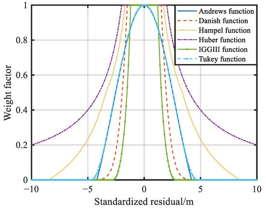
Figure 1.
The weight factor of different robust estimation functions.
The equivalent weight function discussed in Section 2.2 is substituted into Equation (8) for iterative calculation to solve the position parameters [38].
where represents the iteration, and represents the number of redundant observations.
In this paper, when the difference between the position parameters calculated in the two consecutive iterations meets the convergence accuracy, the calculation is stopped.
The flowchart of the proposed algorithm is shown in Figure 2. The process can be summarized as follows: the data of base station and mobile station are used to estimate parameters. The high-quality observations are selected on the basis of the SNR to build the subset of the WL ambiguity, and the ratio value and unit weight of standard error are used to confirm the ambiguity. The WL equations of low-quality observations are constructed by the constraint of the fixed WL ambiguity, and the robust estimation is used to solve the residual WL ambiguities. The LAMBDA algorithm is used to search integer ambiguities, and the ratio value and unit weight of standard error are used to confirm the integer ambiguity. The basic ambiguities are solved according to the relationship between the wide-lane observation equation and the basic observation equation, and the fixed basic ambiguities are substituted into the observation equation to solve the position parameters. The robust estimation is used to reduce the effects of outliers for position parameter estimation.
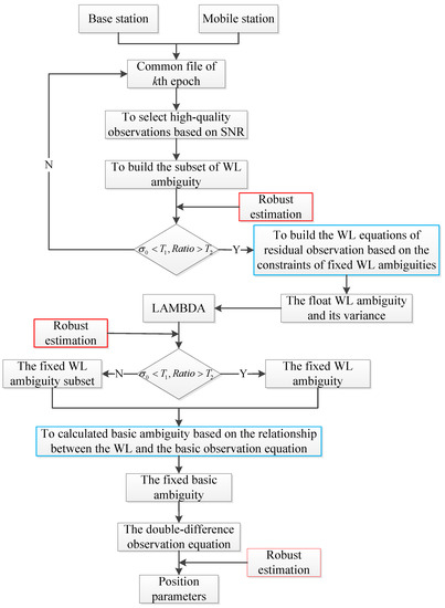
Figure 2.
Process flow of the proposed method.
3. Results
A NovAtel ProPak6 receiver was used to collect static and dynamic data to analyze the performance of the proposed algorithm. Seven schemes were designed, and self-development programs were used to analyze these data. Scheme 1 was a robust estimation based on the Andrews function. Scheme 2 was a robust estimation based on the Danish function. Scheme 3 was a robust estimation based on the Hampel function. Scheme 4 was a robust estimation based on the Huber function. Scheme 5 was a robust estimation based on the IGGIII function. Scheme 6 was a robust estimation based on the Tukey function. Scheme 7 was the method without robust estimation. The combined results of commercial software Inertial Explorer (IE) were used as a reference.
3.1. Case One
Static data were collected in an open environment. The reference station was set up on the roof, and the mobile station was set up on the square. The sample rate of reference station and mobile station was 20 Hz, and the collection time was about 3.0 h. These receivers collected data from GPS, GLONASS, and BDS. The data collection environment is shown in Figure 3.
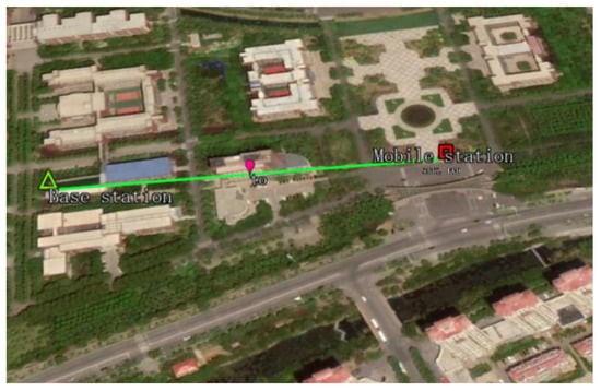
Figure 3.
The environment of the static experiment.
Figure 4 shows the number of visible satellites. In Figure 4, the number of visible satellites was stable during the data collection period, with more than five GPS (G) and GLONASS (R) satellites and more than nine BDS (C) satellites. The number of GPS/GLONASS/BDS (G/R/C) satellites was significantly higher than that of a single-satellite system, with the average number of G/R/C satellites increasing to more than 20.
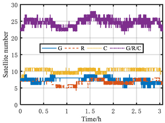
Figure 4.
The number of visible satellites.
The static data were solved by self-development programs, and the combined results of GNSS RTK of IE were used as a reference. Table 1 shows the solution rate of the seven schemes for the static data. The solution rate was the ratio of the solved epoch number of the proposed schemes to the actual epoch number. As shown in Table 1, the solution rate of the seven schemes was the same, reaching 100% regardless of whether the robust estimation was used, due to the good quality of observations.

Table 1.
The solution rate of the seven schemes for the static data.
Figure 5 shows the RMS of the position errors of several proposed schemes in the N, E, and U directions. As shown in Figure 4, the RMS of Scheme 7 (without the robust estimation) could achieve centimeter-level accuracy, at 0.0052 m, 0.0059 m, and 0.0108 m in the N, E, and U directions, respectively. The position accuracy of the robust schemes was basically the same, which was equivalent to Scheme 7 in the horizontal direction and slightly worse than Scheme 7 in the U direction. This is because the high-quality observations were also downweighted or were eliminated when these robust schemes were used in some epochs, which reduced the effect of high-quality observations for the position solution.
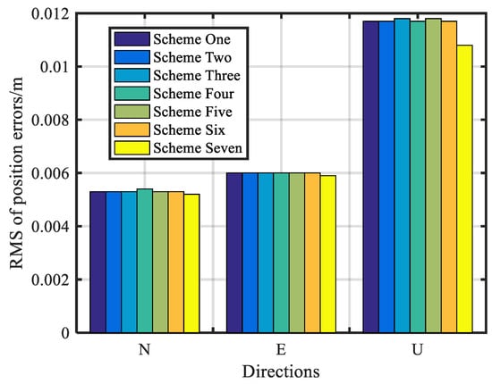
Figure 5.
RMS of the position errors of different schemes.
Table 2 shows the epoch numbers of the ambiguity initialization of several schemes for the static data. As shown in Table 2, Scheme 7 required 186 epochs to fix the ambiguity, while the robust schemes only required a single epoch to fix the ambiguity. The fixed time of ambiguity initialization was improved by more than 99%. Therefore, the robust estimation method could effectively shorten the fixed time of the ambiguity.

Table 2.
Epoch numbers of the ambiguity initialization of several schemes for the static data.
To analyze the performance of different robust schemes to resist outliers, small and large gross errors were simulated in observations. Table 3 shows the epoch and size of the simulated gross errors.

Table 3.
Epoch and size of the simulated gross errors.
The outlier numbers of 1, 3, 6, 9, and 12 were simulated in observations. Specifically, one outlier was simulated in observations of GPS, and one outlier, two outliers, three outliers, and four outliers were simulated in observations of GPS, GLONASS and BDS, respectively.
Figure 6 shows the position errors of different schemes of simulated gross error with different numbers and sizes. Figure 6a presents the position errors of Epoch 179,600 where gross error numbers of 0, 1, 3, 6, 9, and 12 were simulated. In this epoch, there were 22 satellites. Figure 6a shows that the GNSS positioning results were not affected when the number of simulated gross error was less than 4, and the positioning error of Scheme 7 increased more than twofold when the observation number of simulated gross error accounted for 27.27% of the total observations. With the increase in the number of gross errors, the position error gradually increased. When the number of the simulated gross error was 9, these proposed robust schemes could resist gross errors. When the number of simulated gross error reached 12, these robust schemes could not effectively deal with outliers. Figure 6b presents the position errors of different schemes of Epoch 180,200. In this epoch, there were 22 satellites. As shown in Figure 6b, the positioning results of Scheme 7 were biased when the number of simulated gross errors was 1. Schemes 1, 2, 5, and 6 could still effectively resist gross errors when the number of simulated gross errors was 9. However, the positioning result was biased when the number of simulated gross errors was 9 for Schemes 3 and 4, and the position errors were abnormal when the number of simulated gross errors was 6 for Scheme 4. Figure 6c presents the position errors of different schemes of Epoch 181,400. In this epoch, the satellite number was 21. As shown in Figure 6c, the positioning results of the robust schemes (except for Scheme 1) had decimeter-level deviation; when the number of simulated gross errors was 9, Scheme 5 had the least position bias. Figure 6d presents the position errors of different schemes of Epoch 182,000. In this epoch, there were 19 satellites. As shown in Figure 6d, the positioning results of Scheme 3 and Scheme 4 were biased when the number of simulated gross errors was 6. When the observation number of simulated gross errors accounted for 47.37% of the total observations, none of the robust schemes could resist gross errors. Figure 6e presents the position errors of different schemes of Epoch 182,600. In this epoch, there were 21 satellites. As shown in Figure 6e, when the number of simulated gross errors was 6, the robust schemes (except Scheme 3 and Scheme 4) could effectively resist gross errors. When the number of simulated gross errors reached 9, these proposed robust schemes could not resist gross errors. Figure 6f presents the position errors of different schemes of Epoch 183,200. In this epoch, there were 23 satellites. In Figure 6f, when the number of simulated gross errors was 6, the robust schemes (except Scheme 4) could effectively resist gross errors. When the number of simulated gross errors was 9, robust schemes (except Scheme 1) could not resist gross errors.
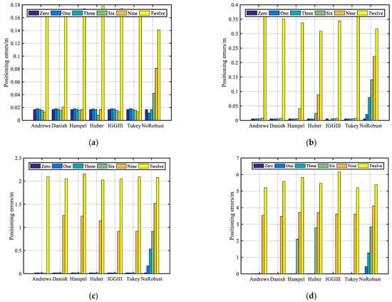
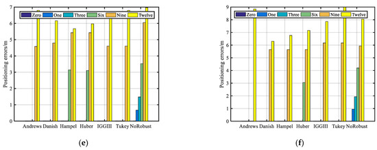
Figure 6.
Position errors of different schemes of simulated gross error with different numbers and sizes: (a) Epoch 179600; (b) Epoch 180,200; (c) Epoch 181,400; (d) Epoch 182,000; (e) Epoch 182,600; (f) Epoch 183,200.
In conclusion, the scheme without robust estimation could still obtain centimeter-level results when the observation number of the simulated 0.5-cycle gross error accounted for less than 13.64% of the total observations. Several robust schemes could effectively resist gross errors when the observation number of simulated gross errors accounted for 40.91% of the total observations. The robust performance of Scheme 4 was reduced when the observation numbers of the simulated one-cycle gross error accounted for 27.27% of the total observations. The robust performance of Schemes 3 and 4 was reduced when the observation numbers of simulated gross errors accounted for 40.91% of the total observations, but the position error was still at the centimeter level. Several robust schemes could still effectively resist gross errors when the observation number of the simulated five-cycle gross error accounted for 28.57%. For the simulated large gross errors of more than 10 cycles, the robust performance of Scheme 3 and Scheme 4 was slightly worse, the performance of other schemes was similar, and Scheme 1 was slightly better. Therefore, the robust effect of Schemes 3 and 4 was slightly worse for the simulated multiple gross errors.
3.2. Case Two
In urban environments, dynamic data were collected by the vehicle-born surveying system researched and development by Shandong University of Science and Technology and the company of Supersurs. The vehicle system is shown in Figure 7, and it was equipped with multiple sensors. The reference station was set up on the roof, and the mobile station was carried on the vehicle. The data included those from GPS, GLONASS, and BDS. The sample rate was 20 Hz, and the collection time was about 2.8 h. There were many blocked environments, including tall buildings, viaducts, tall porches, and shady roads. The experimental area and mobile trajectory are shown in Figure 8. In Figure 8, the marked A is the experimental area of signal interference, B is the experimental area of densely built, C is the experimental area of viaduct, and D is the experimental area of tall porch area.
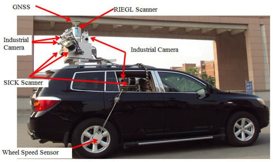
Figure 7.
Vehicle-borne surveying system.
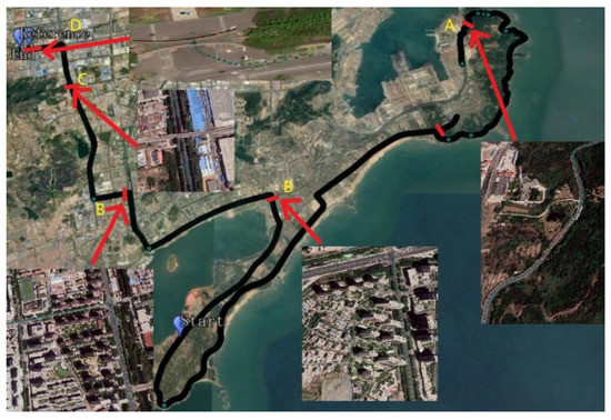
Figure 8.
Experimental area and mobile trajectory.
Figure 9 shows the number of visible satellites. In Figure 9, the satellite number of GPS was more than five, the satellite number of GLONASS was more than four, and the satellite number of BDS was more than eight most of the time. The number of GPS/GLONASS/BDS satellites was significantly higher than that of the single-satellite system, and the number of GPS/GLONASS/BDS satellites reached 15 most of the time. However, the satellite number of GNSS was less than four in some blocked environments.
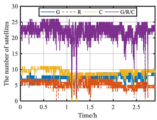
Figure 9.
The number of satellites.
The self-development programs were used to solve the data, and the combined smoothed results of GNSS RTK/INS integrated navigation of IE were used as a reference. Table 4 shows the solution rate of the seven schemes for the dynamic data. As shown in Table 4, the solution rate of Scheme 7 (where robust estimation was not used) was 97.83%, while the solution rate of several robust schemes was improved to more than 99%. The solution rate of Scheme 6 reached 99.57%, and the improvement effect of the solution rate was the best. This was followed by Scheme 5 with a solution rate of 99.47%, while the solution rate of Scheme 1 also reached 99.35%.

Table 4.
The solution rate of the seven schemes for the dynamic data.
Table 5 shows the epoch numbers of ambiguity initialization of several schemes for the dynamic data. As shown in Table 5, 48 epochs were needed to fix the ambiguity for Scheme 7, while the ambiguity could be fixed by a single epoch when robust estimation was used. The fixed time of ambiguity initialization was improved by more than 97.92%. Thus, the robust estimation method could effectively shorten the fixed time of the ambiguity initialization.

Table 5.
The epoch numbers of ambiguity initialization of several schemes for the dynamic data.
Figure 10 shows the position error of these proposed schemes. In Figure 10a, the area marked A is the signal interference area, B is the densely built area, C is the viaduct area, and D is the tall porch area. The actual environments of these marked areas are shown in Figure 8. Figure 11 shows the 3D position errors of the marked areas in Figure 10a. Figure 10 and Figure 11a show that Scheme 7 could not obtain the positioning results during a period of time in the area marked A, and the positioning results had decimeter-level errors in A. The positioning accuracy and solution rate were improved by robust schemes, and there were still decimeter-level errors for all robust Schemes in A. Figure 9 shows that the number of satellites during this period of time was low. The weight functions of Schemes 1 and 6 included a weight reduction segment and elimination segment. The low-quality satellites were directly eliminated such that the number of satellites participating in the position calculation was low and the reliability of positioning results was reduced. Figure 10 and Figure 11b show that Scheme 7 had continuous decimeter errors in the area marked B, and the position errors were reduced to the centimeter level by robust schemes. As shown in Figure 10 and Figure 11c, Scheme 7 had decimeter errors, and the position could not be obtained at some moments in the area marked C. The position accuracy was greatly improved when robust estimation was used, and Schemes 4 and 5 had a better improvement effect. As shown in Figure 10 and Figure 11d, Scheme 7 failed to obtain the position results for a long time in the area marked D, and the solution rate was improved by the robust schemes. Due to the serious blocked environment, several robust schemes also had decimeter-level errors; in Schemes 1 and 6, the decimeter-level errors were large, whereas, in Schemes 3 and 5, the decimeter errors were small.
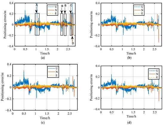
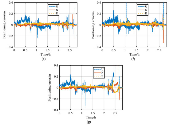
Figure 10.
Position errors of different schemes: (a) Scheme 1; (b) Scheme 2; (c) Scheme 3; (d) Scheme 4; (e) Scheme 5; (f) Scheme 6; (g) Scheme 7.
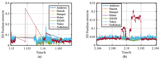
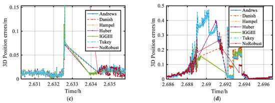
Figure 11.
The 3D position errors of blocked environments of different schemes: (a) signal interference area; (b) densely built area; (c) viaduct area; (d) tall porch area.
Table 6 shows the accuracy statistics of the position errors of the proposed schemes shown in Figure 10. As shown in Table 6, the RMS of the position errors of Scheme 7 was 0.0203 m, 0.0279 m, and 0.1685 m in the N, E, and U directions, respectively, and the maximum 3D position error reached 0.8113 m. The position accuracy was significantly improved by robust schemes. The RMS values of the 3D position error for the six robust schemes were 0.0516 m, 0.0493 m, 0.0495 m, 0.0496 m, 0.0494 m, and 0.0516 m. Compared with Scheme 7, the RMS of the six robust schemes was improved by 70.00%, 71.34%, 71.22%, 71.16%, 71.28%, and 70.26%, respectively. The maximum 3D position error was improved by these robust schemes. Scheme 5 had the best improvement effect, with the maximum 3D position error reduced to 0.2544 m, while the improvement effect of Schemes 1 and 6 was slightly worse.

Table 6.
The accuracy statistics of position errors of proposed schemes.
Figure 12 shows the cumulative probability of the position errors of the proposed schemes. As shown in Figure 12, the probability of Scheme 7 was only 63.18% when the 3D position error was less than 0.05 m. The cumulative probability was improved by the robust schemes. The cumulative probability of Scheme 5 reached 71.83%, of Scheme 2 reached 71.68%, and of other robust schemes reached more than 70%. The cumulative probability of Scheme 7 was only 86.98% when the 3D position error was less than 0.10 m, and the probability of several robust schemes reached more than 94%, among which Schemes 2 and 4 reached 94.84%, and Scheme 5 reached 94.64%. The cumulative probability of Scheme 7 was only 90.51% when the 3D position error was less than 0.15 m, and the probability of several robust schemes reached more than 98%, among which Scheme 5 had the best effect with a probability of 99.15%, followed by Scheme 6 at 99.13%. Compared with Scheme 7, the cumulative probability of the position error was also improved by several robust schemes for other position error intervals.
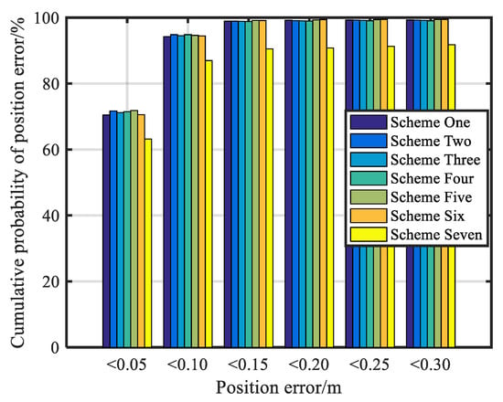
Figure 12.
The cumulative probability of the position errors of the proposed schemes.
Table 7 shows the average number of iterations of the proposed robust schemes. In this paper, the iteration calculation was terminated when the position difference of two consecutive iterations was less than a certain threshold. As shown in Table 7, the average number of iterations of Schemes 1 and 6 was more than 200, and the average number of iterations of Schemes 3 and 4 was also more than 30. The average number of Schemes 2 and 5 was less, being only 11.3081 for Scheme 5. Therefore, Scheme 5 had the smallest computational burden among the proposed robust estimation schemes in this paper.

Table 7.
The average number of iterations of proposed robust schemes.
4. Discussion
In this study, the proposed strategy of GNSS positioning could obtain reliable and high-accuracy position parameters in urban blocked environments. Compared with methods without robust estimation, the performance of GNSS positioning was improved by robust schemes. Scheme 5 had the best performance among the proposed robust schemes with regard to the positioning performance and computational efficiency. The positioning performance of the proposed algorithm was analyzed on the basis of data collected in urban environments, and decimeter-level or centimeter-level positioning results could be obtained by the proposed algorithm when gross errors occurred in observations. Centimeter-level positioning accuracy could still be obtained by the proposed strategy when observation numbers of the simulated 15-cycle gross error accounted for 28.75% of the total observations. Therefore, a continuous and high-accuracy position reference can be provided for mapping by the proposed algorithm, which can promote the development of mobile mapping systems and intelligent driving in urban environments.
5. Conclusions
In a complex urban environment, the reliability of GNSS positioning has numerous requirements, and GNSS signals are susceptible to the interference from block environments, resulting in a reduction in the observation quality, which affects the accuracy and reliability of GNSS positioning. Therefore, we proposed an algorithm of GNSS reliable positioning with several robust schemes. The technology of double-difference GNSS RTK was used to discuss the proposed algorithm, and the least squares method was used to solve parameters. The partial ambiguities method was used to solve the ambiguities. Different equivalent weight functions of robust estimation were analyzed, and the designed schemes of robust estimation were used to reduce the influence of the residual errors and uncorrected ambiguities for high-accuracy positioning. Static and dynamic data were used to assess the performance of the proposed algorithm. Some conclusions can be drawn from our experiments:
Firstly, reliable results of GNSS positioning can be obtained regardless of whether robust estimation is used in the open environment, and the accuracy and solution rate can be improved by the robust scheme in blocked environments.
Secondly, the fixed time of the ambiguity initialization can be significantly improved by robust schemes. Several robust schemes can effectively resist the simulated small and large gross errors.
Thirdly, to consider the positioning performance and computational efficiency, the IGGIII scheme that includes the three-segment function is more effective than other proposed robust schemes in complex blocked environments.
Author Contributions
Methodology, software, and writing—original draft preparation, D.C.; conceptualization, validation, and writing—review and editing, Y.N.; investigation and formal analysis, S.W., W.S. and J.X.; investigation and data curation, J.B. All authors have read and agreed to the published version of the manuscript.
Funding
This work was supported by the Natural Science Foundation of Shandong Province (grant numbers ZR2022QD108 and ZR2021QD058), the National Natural Science Foundation of China (grant numbers 42204011 and 42001397), the Doctoral Research Fund Program of Shandong Jianzhu University (grant number X21066Z), the National Key Research and Development Program of China (grant number 2021YFB1407001), the Key R&D Project of Shandong Province (grant number 2019GSF111052), and the Higher Educational Science and Technology Program of Shandong Province (grant number J17KA071).
Data Availability Statement
The data presented in this study are available on request from the authors on reasonable request.
Acknowledgments
The authors thank the reviewers and editor for their constructive and valuable comments, which helped greatly in revising the paper.
Conflicts of Interest
The authors declare no conflict of interest.
References
- Chai, D.S.; Wang, S.L.; Lu, X.S.; Shi, B. The research of high-frequency single—Epoch GNSS kinematic differential positioning technology. In Proceedings of the CSNC2016, China Satellite Navigation Conference (CSNC) 2016 Proceedings, Changsha, China, 18–20 May 2016; Springer: Singapore, 2016; pp. 85–95. [Google Scholar]
- Guo, J.; Zhang, Q.Y.; Li, G.C.; Zhang, K.L. Assessment of multi-frequency PPP ambiguity resolution using Galileo and Bei-Dou-3 Signals. Remote Sens. 2021, 13, 4746. [Google Scholar] [CrossRef]
- Paziewski, J.; Sieradzki, R. Integrated GPS+BDS instantaneous medium baseline RTK positioning: Signal analysis, methodology and performance assessment. Adv. Space Res. 2017, 60, 2561–2573. [Google Scholar] [CrossRef]
- Geng, J.H.; Chang, H.; Guo, J.; Li, G.C.; Wei, N. Three multi-frequency and multi-system GNSS high-precision point positioning methods and theis performance in complex urban environment. Acta Geod. Cartogr. Sin. 2020, 49, 1–13. [Google Scholar]
- Zhang, X.H.; Pan, Y.M.; Zuo, X.; Wang, J. An improved robust kalman filtering and its application in PPP. Geomat. Inf. Sci. Wuhan Univ. 2015, 40, 858–864. [Google Scholar]
- Aboutaleb, A.; El-Wakeel, A.S.; Elghamrawy, H.; Noureldin, A. LiDAR/RISS/GNSS dynamic integration for land vehicle robust positioning in challenging GNSS environments. Remote Sens. 2020, 12, 2323. [Google Scholar] [CrossRef]
- Knight, N.L.; Wang, J.L. A comparison of outlier detection procedures and robust estimation methods in GPS positioning. J. Navig. 2009, 62, 699–709. [Google Scholar] [CrossRef]
- Yang, L.; Wang, J.; Knight, N.L.; Shen, Y. Outlier separability analysis with a multiple alternative hypotheses test. J. Geod. 2013, 87, 591–604. [Google Scholar] [CrossRef]
- Yu, H.J.; Shen, Y.Z.; Yang, L.; Nie, Y.F. Robust M-estimation using the equivalent weights constructed by removing the influence of an outlier on the residuals. Surv. Rev. 2019, 51, 60–69. [Google Scholar] [CrossRef]
- Yang, C.; Shi, W.Z.; Chen, W. Robust M-M unscented kalman filtering for GPS/IMU navigation. J. Geod. 2019, 93, 1093–1104. [Google Scholar] [CrossRef]
- Zhou, J.W. Classical theory of errors and robust estimation. Acta Geod. Cartogr. Sin. 1989, 18, 115–120. [Google Scholar]
- Yang, Y.X.; Cheng, M.K.; Shum, C.K.; Tapley, B.D. Robust estimation of systematic errors of satellite laser range. J. Geod. 1999, 73, 345–349. [Google Scholar] [CrossRef]
- Yang, Y.X.; Song, L.; Xu, T.H. Robust estimator for correlated observations based on bifactor equivalent weights. J. Geod. 2002, 76, 353–358. [Google Scholar] [CrossRef]
- Wang, Y.D.; Sun, S.M.; Li, L. Adaptively robust unscented kalman filter for tracking a maneuvering vehicle. J. Guid. Control Dyn. 2014, 37, 1696–1701. [Google Scholar] [CrossRef]
- Guo, F.; Zhang, X.H. Adaptive robust kalman filtering for precise point positioning. Meas. Sci. Technol. 2014, 25, 105011–105018. [Google Scholar] [CrossRef]
- Yang, L.; Shen, Y.Z. Robust M estimation for 3D correlated vector observations based on modified bifactor weight reduction model. J. Geod. 2020, 94, 31–47. [Google Scholar] [CrossRef]
- Bahadur, B.; Nohutcu, M. Integration of variance component estimation with robust kalman filter for single-frequency multi-GNSS positioning. Measurement 2021, 173, 108596–108606. [Google Scholar] [CrossRef]
- Zhang, Q.Q.; Zhao, L.D.; Zhao, L.; Zhou, J.H. An improved robust adaptive kalman filter for GNSS precise point positioning. IEEE Sens. J. 2018, 18, 4176–4186. [Google Scholar] [CrossRef]
- Fan, P.R.; Li, W.Y.; Cui, X.W.; Lu, M.Q. Precise and robust RTK-GNSS positioning in urban environments with dual-antenna configuration. Sensors 2019, 19, 3586. [Google Scholar] [CrossRef]
- Wang, Q.X.; Xu, T.H.; Xu, G.C. Application of combining method of outlier detection and robust estimation to GPS kinematic relative positioning. Geomat. Inf. Sci. Wuhan Univ. 2011, 36, 476–480. [Google Scholar]
- Wang, S.L.; Wang, Q.; Pan, S.G.; Yu, X.X. Double integer ambiguities test an repair method netwok RTK base stations based on robust estimation. J. Chin. Inert. Technol. 2012, 20, 705–714. [Google Scholar]
- Pan, C.; Qian, N.J.; Li, Z.K.; Gao, J.X.; Liu, Z.B.; Shao, K.F. A robust adaptive cubature kalman filter based on SVD for dual-antenna GNSS/MIMU tightly coupled integration. Remote Sens. 2021, 13, 1943. [Google Scholar] [CrossRef]
- Gaglione, S.; Innac, A.; Carbone, S.P.; Troisi, S.; Angrisano, A. Robust estimation methods applied to GPS in harsh environments. In Proceedings of the 2017 European Navigation Conference (ENC), Lausanne, Switzerland, 9–12 May 2017; pp. 14–25. [Google Scholar]
- Crespillo, O.G.; Andreetti, A.; Grosch, A. Design and evaluation of robust M-estimators for GNSS positioning in urban environments. In Proceedings of the 2020 International Technical Meeting of The Institute of Navigation, San Diego, CA, USA, 21–24 January 2020; pp. 1–14. [Google Scholar]
- Han, H.Z.; Wang, J. Robust GPS/BDS/INS tightly coupled integration with atmospheric constraints for long-range kinematic positioning. GPS Solut. 2017, 21, 1285–1299. [Google Scholar] [CrossRef]
- Chai, D.S.; Sang, W.G.; Chen, G.L.; Ning, Y.P.; Yu, M.W.; Wang, S.L. A novel method of ambiguity resolution and cycle slip processing for single-frequency GNSS/INS tightly coupled integration system. Adv. Space Res. 2022, 69, 359–375. [Google Scholar] [CrossRef]
- Shi, J.B.; Huang, Y.H.; Ouyang, C.H. A GPS relative positioning quality control algorithm considering both code and phase observation errors. J. Geod. 2019, 93, 1419–1433. [Google Scholar] [CrossRef]
- Li, Z.; Xu, G.L.; Guo, J.; Zhao, Q.L. A sequential ambiguity selection strategy for partial ambiguity resolution during RTK positioning in urban areas. GPS Solut. 2022, 26, 92–107. [Google Scholar] [CrossRef]
- Liu, W.K.; Li, J.L.; Zeng, Q.; Guo, F.; Wu, R.P.; Zhang, X.H. An improved robust kalman filtering strategy for GNSS kinematic positioning considering small cycle slips. Adv. Space Res. 2019, 63, 2724–2734. [Google Scholar] [CrossRef]
- Wang, S.L.; Deng, J.; Lu, X.S.; Song, Z.Y.; Xu, Y. A new GNSS single-epoch ambiguity resolution method based on triple-frequency signals. Isprs. Int. J. Geo-Inf. 2017, 6, 46. [Google Scholar] [CrossRef]
- Odolinski, R.; Teunissen, P.J.G.; Odijk, D. Combined GPS+BDS for short to long baseline RTK positioning. Meas. Sci. Technol. 2015, 26, 1–16. [Google Scholar] [CrossRef]
- Chai, D.S.; Chen, G.L.; Wang, S.L.; Lu, X.S. A new single-epoch method for resolving GNSS ambiguity with segmented search in short baseline. Adv. Space Res. 2018, 62, 30–43. [Google Scholar] [CrossRef]
- Brunner, F.; Hartinger, H.; Troyer, L. GPS signal diffraction modelling: The stochastic SIGMA-δ model. J. Geod. 1999, 73, 259–267. [Google Scholar] [CrossRef]
- Andrews, D.F. A robust method for multiple linear regression. Technometrics 1974, 16, 523–531. [Google Scholar] [CrossRef]
- Huber, P.J. Robust estimation of a location parameter. Ann Math Stat. 1964, 35, 73–101. [Google Scholar] [CrossRef]
- Baselga, S. Global Optimization Solution of Robust Estimation. J. Surv. Eng. 2007, 133, 123–128. [Google Scholar] [CrossRef]
- Beaton, A.E.; Tukey, J.W. The fitting of power series, meaning polynomials, illustrated on band-spectroscopic data. Technometrics 1974, 16, 147–185. [Google Scholar] [CrossRef]
- Yu, X.X.; Lv, W.C. Robust estimation model for correlated observations based on standardized residuals. Inf. Sci. Wuhan Univ. 1998, 24, 75–78. [Google Scholar]
Publisher’s Note: MDPI stays neutral with regard to jurisdictional claims in published maps and institutional affiliations. |
© 2022 by the authors. Licensee MDPI, Basel, Switzerland. This article is an open access article distributed under the terms and conditions of the Creative Commons Attribution (CC BY) license (https://creativecommons.org/licenses/by/4.0/).