Abstract
With the growth of cloud computing, the use of the Google Earth Engine (GEE) platform to conduct research on water inversion, natural disaster monitoring, and land use change using long time series of Landsat images has also gradually become mainstream. Landsat images are currently one of the most important image data sources for remote sensing inversion. As a result of changes in time and weather conditions in single-view images, varying image radiances are acquired; hence, using a monthly or annual time scale to mosaic multi-view images results in strip color variation. In this study, the NDWI and MNDWI within 50 km of the coastline of the Yucatán Peninsula from 1993 to 2021 are used as the object of study on GEE platform, and mosaic areas with chromatic aberrations are reconstructed using Landsat TOA (top of atmosphere reflectance) and SR (surface reflectance) images as the study data. The DN (digital number) values and probability distributions of the reference image and the image to be restored are classified and counted independently using the random forest algorithm, and the classification results of the reference image are mapped to the area of the image to be restored in a histogram-matching manner. MODIS and Sentinel-2 NDWI products are used for comparison and validation. The results demonstrate that the restored Landsat NDWI and MNDWI images do not exhibit obvious band chromatic aberration, and the image stacking is smoother; the Landsat TOA images provide improved results for the study of water bodies, and the correlation between the restored Landsat SR and TOA images with the Sentinel-2 data is as high as 0.5358 and 0.5269, respectively. In addition, none of the existing Landsat NDWI products in the GEE platform can effectively eliminate the chromatic aberration of image bands.
1. Introduction
In recent decades, satellite imagery has developed, representing an effective source to monitor natural resources [1], vegetation ecological inversions [2], ecological function [3], and land–sea interactions [4]. High-quality satellite images normally need to satisfy three criteria for efficient operation: high-quality mosaic, abundant information, and harmonious tones [5]. Satellite images are inevitably affected by external disturbances, including seasonal variations and diverse atmospheric conditions, as well as internal elements, such as sensors and the satellite re-entry cycle during the image capture process, which all lead to uneven light distribution in satellite images [6,7]. Especially in large-scale satellite monitoring of long time series, it is frequently necessary to compare multi-period remote sensing images in order to distinguish the factors in response to the problem of different grayscale values of images and the phenomenon of uneven hue of adjacent image strips, such as changes in features, as well as image data mosaicked in different time scales, such as monthly, quarterly, and annual.
Google Earth Engine (GEE) is a cloud platform for satellite image visualization, calculation, and analysis at a planetary scale. A large number of studies have been deployed using GEE, including disaster monitoring [8], vegetation change [9,10], urban expansion [11], and land cover analysis [12]. The GEE platform brings together more than 600 datasets, including Landsat, MODIS, Sentinel, and a large number of multi-spectral satellite images, facilitating the work of researchers [13]. Increasing trends can be observed in long time series NDWI and MNDWI analysis, as well as online visualization at a large scale [14,15,16]. NDWI is a fundamental index used to monitor climate changes that have induced water body change and to evaluate the impact of economic development on inland aquatic ecosystems [17]. NDWI has a clear advantage in assessing the relationship between surface water and seasonal precipitation [18,19]. When using NDWI for water body assessment, images of mountain shadows and clouds are easily received, and the results are prone to inaccuracy [20]. MNDWI is a modified normalized difference water index that enhances open water features [21]. Long-term monitoring of changes in coastal shorelines using MNDWI based on long-term of Landsat image series can effectively identify coastal erosion and coastal exploration. Dynamic monitoring of shorelines and tidal flats using Landsat image inversion for MNDWI could be a suitable indicator for sustainable development analysis [22]. The NDWI is commonly used to extract the body of water part of images [23]. However, the MNDWI is more accurate in built-up areas [24]. Moreover, the existing NDWI analyses over long time series often do not address the striping problems caused by image mosaics.
There has recently been an increased focus on the color leveling of remote sensing images. For instance, the Wallis method of filtering is used to differentiate areas of images with similar mean and variance; GeoDodging software employs this method to align the color and brightness of different images [25]. The histogram-matching method can be applied to a single image or image overlap area as a reference and change other images to be restored in the image mosaic process for color leveling, which is a typical non-linear image restoration method [26]. Color correction in ArcGIS software is based on the idea of gamma correction for image leveling in the survey area, which is based on the principle of interpolation of the correction parameters of non-overlapping areas from the overlapping areas of an image [27]. The above methods can be effective for color leveling studies of similar features in multi-scene images; however, for a wide range of image coverage with multiple image strips with inconsistent color differences in a given area, using the above image restoration methods causes overall tonal distortion. Currently available methods do not consider the position relationship between images and cause cumulative errors in color transfer when used in long-term analyses.
Mainstream machine learning methods include SVM (support vector machine), neural networks, random forests, etc. SVM can only achieve small-scale sample training and binary classification with a significant effect [28]. A neural network is a typical gradient algorithm that solves the global extrema of complex nonlinear functions, with highly randomized training accuracy depending on the selected network and the quality of training samples [29]. Compared with other machine learning methods, random forest methods can provide mutually independent training subsets without feature selection and can achieve fast parallelization of high-dimensional and complex training data [30]. Random forest methods are widely used for remote sensing image classification, natural resource surveying, and environmental monitoring [31] but are rarely used for image restoration; therefore, in this paper, we adopt random forest methods for image restoration.
Three primary issues need to be addressed in the afterglow processing of remote sensing images with grayscale values of existing multi-view images to improve understanding of long-term NDWI and MNDWI indices. First, in the study of strip color differences caused by stitching of medium and large-scale multi-view images, it is difficult for existing leveling algorithms to achieve basic consistency in terms of brightness and hue among image strips after processing [6]. Second, in long-term time series remote sensing monitoring, the image restoration rules based on multi-source remote sensing are inconsistent and cannot effectively guarantee the objectivity of current image quality and the accuracy of long-term image inversion [32,33]. Third, an automatic and robust method is needed to implement batch processing of large amounts of image restoration for the homogenization of medium- and large-scale remote sensing images of long-term time series [5,34]. Therefore, there is an urgent need to solve the problem of how to efficiently and rapidly achieve restoration using current homologous remote sensing images in long time series and medium- and large-scale remote sensing image homogenization processes.
To address the above issues, in the present study, we employed a random forest algorithm to quickly classify the DN values and probabilities of the images separately based on the GEE platform; the classified results were then matched in a histogram. In this study, two water body indices, NDWI and MNDWI, were analyzed using Landsat TM/OLI image band computing from 1993 to 2021, and the results of image restoration were compared with existing Landsat, MODIS, and Sentinel-2 products to verify the effectiveness of the method. We propose a machine-learning-based histogram image restoration method that can provide a theoretical foundation for the homogenization study of long time series large-scale images.
2. Materials and Methods
2.1. Study Area
The Yucatán Peninsula (18°50′42″N, 89°07′32″W) is a peninsula located in northern Central America and southeastern Mexico [35], separating the Caribbean Sea from the Gulf of Mexico [36]. It is bordered by the Caribbean Sea to the east, the Gulf of Mexico and the Bay of Campeche to the west, and Cuba across the Yucatán Strait to the northeast, with an area of 197,600 square kilometers. The Yucatán Peninsula has an average elevation of less than 200 m, with a high southern and low northern topography. The average width of the peninsula is approximately 320 km, and its coastline is approximately 1100 km long [37]. The area analyzed in the present study is within 50 km of coast of the Yucatán Peninsula, as shown in Figure 1.

Figure 1.
Location of the study area. (a) Location of Yucatán Peninsula in Mexico; (b) path and row of each Landsat image. (WRS PATH:18–21 WRS ROW:45–48).
The climate of the Yucatán Peninsula is tropical, ranging from semiarid in the north to humid in the south. The average annual precipitation varies from less than 800 mm in the driest regions of the northwest to 2000 mm in the southern Petén Basin. Rainfall varies seasonally, with August and September generally representing the wettest months. As one of the largest karst landscapes in the world, the Yucatán Peninsula provides a suitable habitat for mangrove growth, with a carbon stock of more than 1000 Mg C ha-1 [38]. The carbon stocks in the Sian Ka’an Biosphere Reserve store the equivalent of approximately 185.7 million Mg CO2e, which is equivalent to almost half (40–46%) of the carbon emissions of Mexico in 2009 (399.7 million Mg of CO2e) [39]. Mangroves have the potential to help regulate the atmosphere, particularly by reducing atmospheric carbon concentrations and sequestering carbon stocks [40].
Due to the extreme karst nature of the whole peninsula, the northern Yucatán Peninsula is devoid of rivers. Where lakes and swamps are present, the water is typically marshy and generally unpotable [41]. Dry forests occupy the dry northwestern peninsula and include dry forests and scrublands, as well as cactus scrub. Moist forests occupy the middle and eastern portions of the peninsula and are characterized by semi-deciduous forests, where 25% to 50% of the trees lose their leaves during the summer dry season. Belizean pine forests are found in several enclaves across central Belize. The southernmost portion of the peninsula is in the Petén–Veracruz moist forests ecoregion, an evergreen rain forest [42].
2.2. Data and Processing
2.2.1. Image Collection
To reduce the images of Landsat 7 ETM data strips for image analysis, we primarily used Landsat 5 TM and Landsat 8 OLI data, with experimental data obtained from the GEE cloud platform. By screening the images of the study area, it is found that the Landsat 5 TM dataset from 1984 to 2012 did not include images for 1988, 2004, 2005, or 2006. A large number of images were missing for 2010, 2009, 2008, 2007, 2003, 2002, 1992, 1991, 1990, and 1989. Complete Landsat 5 TM were available for 1993 to 2001, and complete Landsat 8 OLI date were available for 2013 to 2021. The NDWI synthetic products available on GEE (ANNUAL, 32-DAY, 8-DAY, and MODIS) and the NDWI images after the Sentinel-2 band operation were also used as a dataset for comparison and validation. The range of Landsat image ranks in the study area is: World Reference System (WRS) PATH: 18–21, WRS_ROW: 45–47. A summary of image data details is shown in Table 1.

Table 1.
List of Landsat, MODIS, and Sentinel-2 image data used in this study.
2.2.2. Image Processing
Figure 2 depicts the technical process employed in this study, which is divided into four steps. The first step is image preprocessing, which includes (1) time and boundary screening, (2) cloud and cloud shadow removal, and (3) NDWI and MNDWI calculation to obtain the mosaic image. The preprocessed images were visually evaluated for the presence of strip color differences in the second step; portions with strip color differences were segmented and designated as the target image, and the reference image corresponding to each image was chosen. In the third step, the probability density function and cumulative distribution function were calculated for the NDWI and MNDWI values of each target image and reference image part. In order to obtain the DN values and probability distribution statistics, a classifier was built using a random forest algorithm, taking the DN values of the reference image as a training subset and mapping the training results to the target image. The final step was image analysis, including annual time series image analysis, single-view image analysis, and multi-source remote sensing image comparison analysis.
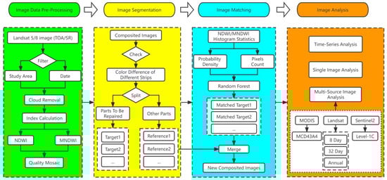
Figure 2.
Overall methodology of the study.
We used the existing technical methods of GEE: (1) normalized index calculation function ee.Image.normalizedDifference(), (2) image filtering boundary filter and time filter functions ee.ImageCollection.filterBounds() and ee.ImageCollection.filterDate(), (3) single-band image mosaic function ee.ImageCollection.qualityMosaic(), and (4) random forest function ee.Classifier.smileRandomForest(). The library of functions called external GEE includes ee-palettes (a module for generation of color palettes in GEE to be applied to mapped data). The main improvements and independently implemented parts are as follows: (1) the removal of clouds and cloud shadows using the QA (pixel_qa) band bit mask technique in Landsat images, (2) the statistical functions (probability distribution function and cumulative distribution function) in each band of the image, (3) the image mapping method using the random forest method, and (4) multi-band image Pearson correlation analysis function.
2.3. Methods
2.3.1. NDWI and MNDWI
NDWI (normalized difference water index) and normalized difference processing with green band and NIR (near infrared) bands of remotely sensed images were used to highlight the water body information in the images [43]. The value range of NDWI is [−1, 1], and DN ≥ 0 of image elements in NDWI generally indicates that the ground is covered by water bodies or dark, bare ground, whereas negative values indicate vegetation coverage [44].
MNDWI is an improved water body index proposed on the basis of the modification normalized difference water index (MNDWI), which is a normalized ratio index based on the near-infrared band and the mid-infrared band. Previous studies have demonstrated that MNDWI achieves better performance than NDWI for water body extraction and can better reveal changes, such as fine features of water bodies [21,23].
2.3.2. Random Forest Algorithm
The random forest algorithm is a machine learning algorithm based on the combination of decision trees proposed by Breiman [45,46]. The construction of a random forest classifier involves two primary aspects: random selection of data and random selection of features [47]. The basic principles of the algorithm are as follows:
- (1)
- Using put-back sampling, the statistical DN values and the probabilities of the reference images serve as the original dataset from which a subset of data is constructed with the same amount of data as the original dataset [48]. The size of each bagging is approximately 1/2 of the original data, and the size of the test dataset is about 1/2 of the original dataset, which is known as the out-of-bag (OOB) data. The above parameters are the default values for the bag fraction parameter of the GEE randomization algorithm.
- (2)
- According to the principle of minimum Gini coefficient, N bagging groups are randomly selected to form N decision trees, and multiple CART decision trees are constructed using the subsets of each node variable after internal splitting to form a random forest [44]; the number of trees selected in this study is 100.
- (3)
- Statistics of image DN values and probability distributions. The magnitude of DN values in each band of the reference image and the target image are counted using the probability distributions function, and the probability distribution of the DN values of the images are counted using the cumulative distribution function to compare the differences between the reference image and the target image. The image DN values and probability distributions are prepared for the next step of random forest classification.
- (4)
- The generated random forest classifier classifies the data. The reference image and the image to be restored are assigned DN values, and their probability distributions are classified by the random forest algorithm according to the above steps in the following process: (1) The DN value classifier of the reference image is derived according to the statistical DN values of each band of the reference image as a training subset using the random forest function. (2) The probability of the DN value of each band of the image to be restored is used as the training subset, and the random forest function is used to derive the probability classifier of the image to be restored. (3) The DN values of the reference image are matched with the DN values of the restored image using the DN value classifier of the reference image to map the probability distribution of the DN values of the reference image to the reference image.
3. Results
In the process of year-by-year NDWI and MNDWI calculations, the inconsistency of strip color difference caused by image mosaic is a common occurrence. The strip color difference of images from 1993–2001 and 2013–2021 were repaired and corrected, respectively. The mean value of NDWI of Landsat TOA images increased from 0.6243 to 0.6280, and the standard deviation of image elements decreased from 0.1302 to 0.1272; the mean value of NDWI of Landsat SR images increased from 0.7042 to 0.7279, whereas the standard deviation of NDWI decreased from 0.2321 to 0.2100. The mean value of the restored MNDWI of Landsat TOA images increased from 0.8790 to 0.8819, and the standard deviation of image elements decreased from 0.0897 to 0.0867; the mean value of the MNDWI of Landsat SR images increased from 0.7565 to 0.7745, and the standard deviation decreased from 0.2328 to 0.2183.
The results of the time-series analysis of NDWI and MNDWI from 1993–2001 and 2013–2021 are shown in Figure 3. The fluctuations of Landsat TOA images before and after restoration are smaller than those of Landsat SR. MNDWI is consistently smoother than NDWI over time, and there are obvious differences between Landsat SR images in 2001 and 2013 in the articulation section. Due to the variances in sensors, picture timing, and climatic circumstances, as well as the various cloud removal techniques used by TOA photographs and SR images, it is also evident that Landsat TM and OIL images differ from one another and because SR images and TOA images use various de-clouding techniques. The R2 of Landsat SR and TOA images after NDWI correction decreased by 0.0450 and 0.0333, respectively, in comparison to that before restoration, whereas the R2 of Landsat SR and TOA images after MNDWI image correction increased by 0.0321 and 0.0405, respectively, compared with that before restoration.
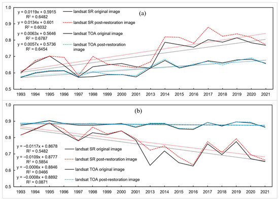
Figure 3.
Time-series analysis. (a) NDWI image; (b) MNDWI image.
3.1. Single-Image Analysis
By analyzing the images year by year, differences between the results of Landsat TM images and OIL images were discovered. To further analyze the effect before and after image restoration, 1998 and 2016 were selected for separate analyses; the restored single-view images are shown in Figure 4 and Figure 5. The results demonstrate that the NDWI and MNDW images after image restoration are smoother without the strip color difference created by the mosaic of single-view images, indicating that the restored images can more accurately depict the desired outcomes.
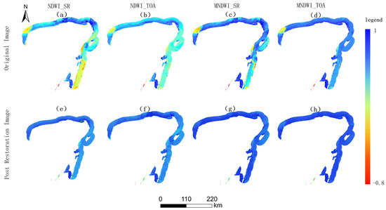
Figure 4.
Before and after image restoration in 1998. (a–d) Original image; (e–h) post-restoration image; (a,e) Landsat SR NDWI image; (b,f) Landsat TOA NDWI image; (c,g) Landsat SR MNDWI image; (d,h) Landsat TOA MNDWI image.

Figure 5.
Before and after image restoration in 2016. (a–d) Original image; (e–h) post-restoration image; (a,e) Landsat SR NDWI image; (b,f) Landsat TOA NDWI image; (c,g) Landsat SR MNDWI image; (d,h) Landsat TOA MNDWI image.
The areas with chromatic aberrations in the 1998 and 2016 images were restored in accordance with the image-stitching stripes, and the mean and standard deviation of NDWI and MNDWI before and after restoration were calculated based on the idea of restoring smaller areas. The statistical results are displayed in Table 2. The standard deviation of the image elements of Landsat SR and TOA images decreased by an average of 0.0283 and 0.0107, respectively, indicating that the effect of using Landsat TOA images for water body index calculation is superior to that of Landsat SR.
Table 2.
Mean values and standard deviations of NDWI and MNDWI of Landsat TOA and SR.
In order to verify the effect of the restored images of the random forest, the area random points of the restored image area and the reference image in 1998 were prepared, with the reference image as the true value and the restored image as the actual value. As shown in Figure 6, the correlations of both the restored image and the reference image are high, whereas the correlations of the Landsat SR image NDWI and MNDWI (R2 = 0.9467 and R2 = 0.9451) are slightly lower than those of Landsat TOA images (R2 = 0.9834 and R2 = 0.9779). In addition, we confirmed that Landsat TOA images were superior to Landsat SR images for restoration purposes.
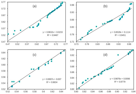
Figure 6.
Scatter plots for the values of NDWI and MNDWI regression equations in 1998. (a) Landsat SR NDWI image; (b) Landsat SR MNDWI image; (c) Landsat TOA NDWI image; (d) Landsat TOA MNDWI image.
3.2. Multi-Source Image Comparison Analysis
To compare the differences between the restored results of the images matched by the random forest method and the existing GEE products, a portion of the restored areas of the 2016 images was selected for the present study. Figure 7 shows a comparison of the results of the restored images of the area to be restored in 2016 with those of the existing products. The restored results of Landsat TOA and SR image NDWI are shown in Figure 7b,c, and the corresponding comparison images are shown in Figure 7d–h; Landsat 8-day, 32-day, and annual images all have varying degrees of band color difference. The results of the restored areas are better than those of the existing Landsat products. It is sufficient to determine, by comparing them to the MODIS products, that the MODIS images lack strip chromatic aberration. The resolution of MODIS is too coarse to determine the presence of noise, making it unsuitable for the study of images of small areas, whereas the results of the Sentinel-2 data are more precise. Compared to the Sentine-2 image, the restored Landsat image has more significant tonal stratification and more accurately reflects the actual condition of the coastline.
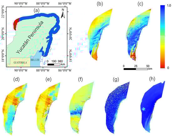
Figure 7.
Comparison of restoration area with different images in 2016. (a) Restoration area in the study area; (b) post-restoration Landsat TOA NDWI image; (c) post-restoration Landsat SR NDWI image; (d) Landsat 8-day NDWI image; (e) Landsat 32-day NDWI image; (f) Landsat annual NDWI image; (g) MOD13Q1 NDWI image; (h) Sentinel-2 NDWI image.
Landsat TOA and SR images of the restored area in 2016 were compared with Landsat 8-day, 32-day, annual, MODIS, and Sentinel 2 results. The statistical results of the differences between the restored images and other data products were determined by comparing the maximum, minimum, mean, and standard deviation of their images of the restored area, as shown in Table 3. Table 4 shows that the NDWI values of the restored Landsat TOA images and the higher-resolution Sentinel-2 images are closer, with mean values of 0.7595 and 0.7499, respectively, and the restored Landsat SR images have a high value of 0.9530, whereas the rest of the Landsat NDWI products are correspondingly low, and the NDWI values of the lower-resolution MODIS products are relatively high. NDWI values are relatively high for the lower-resolution MODIS products.
Table 3.
Statistical analysis of Landsat images, MODIS images, and Sentinel-2 images.
Table 4.
Pearson correlation analysis of NDWI with different images.
Correlation analysis results of the corrected 2016 Landsat images with other data products are presented in Table 4. With the exception of the higher correlation between the restored Landsat TOA and SR images, the highest correlation between the restored Landsat SR images and Sentinel-2 images is 0.5358, followed by the highest correlation between the Landsat TOA images and Sentinel-2 images. The highest correlation is 0.5269, indicating that the results of the restored images are most similar to those of the Sentinel-2 images without strip chromatic aberration, followed by the Landsat annual composite images. Due to the variable degrees of strip chromatic aberration in Landsat’s multiple composites, the findings are less similar.
4. Discussion
In this study, we used the GEE platform to first segment the strip chromatic aberrations in the NDWI and MNDWI image mosaics after the waveform operation and then count the DN values and their probability distributions of the image to be restored and the reference images, respectively, by histogram, and used the random forest function to map the DN values and their probability distributions of the reference image to the image to be restored. The results show that the restored images are superior to the images before the restoration in terms of effectively communicating the desired results. Additionally, the restored images lack any overt banding chromatic aberrations, and the chromatic aberrations are smoother following the image mosaic. In addition, in order to reduce the image restoration process, the total area of the image to be restored was limited to less than 50% of the total of the study area to avoid the results of the restored image from being distorted and thus to improve the image inversion accuracy.
Compared with existing research on image restoration, this study has the following features: 1. In contrast with traditional image restoration techniques based on local ArcGIS and ENVI software, the technique proposed in this study is based on the GEE cloud platform, which can effectively reduce the time spent on image preprocessing and considerably improve the efficiency of image restoration. 2. The principle set out in this study is to restore less than 50% of the area, which can effectively reduce the over-restoration of the image, avoiding distorted image values. 3. The reference image is also the adjacent area of the composite image, which ensures the consistency of the tones of the simultaneous images throughout the restoration process, making it suitable for water index inversion study of long time series synthesized by Landsat, such as monthly, quarterly, and annual.
In this study, we relied on the powerful cloud computing capabilities of the GEE platform, which can determine image DN values and probability distribution statistics using random forest classification and histogram matching in a short period of time. The study process of image restoration does not correlate with the geographical location, topography, and climatic conditions in the study area, and the strip color difference of Landsat’s normalized water body index (NDWI and MNDWI) for long time series is more generalized. The images processed by the algorithm can eliminate the inconsistency of color difference, and there is no obvious difference in tones at the edges of the images. In addition, this algorithm does not encounter the problem of error accumulation caused by color transfer, so it can be used for multiple color leveling according to the hue of each image area to be restored, avoiding images being restored based on the same reference image. The method is suitable for processing the hue inconsistency in the study area because it is larger than the range of single-view images processed with multiple time-phase synthesis.
Restoration was mainly applied in this research using two indices, NDWI and MNDWI, and the indices of other multi-band operations were not analyzed. Further analysis of the indices calculated for other bands is planned in the future to validate and compare the proposed technique with other method among the indices. Although the method proposed in this paper can effectively improve image strip chromatic aberration, the identification of areas where the image strip boundary is not obvious still needs to be improved; in future research, we will focus on the automatic identification and repair of the strip boundary in the study area.
We argue that large areas for Landsat image restoration require significant computational resources and efficient implementation, which was achieved in the present study using the GEE free platform. Because synthetic images of different time scales produce different chromatic aberration areas, the random forest method used in this study is applicable to all areas where image chromatic aberration restoration is required in the process of water surface data processing. In order to verify the regional applicability, we again selected the Southern African Ocean for analysis; the results show that the method is still applicable. The relevant code can be viewed at https://code.earthengine.google.com/13697e3deee07ac64c6da3a69208ed86?hideCode=true, (accessed on 15 August 2022). We also created an app for NDWI image restoration for any region of the world, which can be accessed at https://bqt2000204051.users.earthengine.app/view/landsat5-image--ndwi-restoration, (accessed on 1 October 2020).
5. Conclusions
In this study, we use a random forest algorithm to restore Landsat images with strip chromatic aberrations within 50 km of the coastline of the Yucatán Peninsula for a long time series (1993–2001 and 2013–2021) based on the GEE cloud platform. After restoration, the overlap between the Landsat SR and TOA images is smoother, and in accordance with the principle of minimum image restoration, we propose a new algorithm for the restoration of Landsat images with strip chromatic aberrations. To prevent image distortion and successfully resolve the problem of strip chromatic aberration in single-view image mosaics, the restored area is less than 50 percent.
Our results show that Landsat TOA images produce better results in terms of chromatic aberration and image restoration than Landsat SR images for both the Landsat 5 and Landsat 8 series. The restored Landsat images more accurately depict the actual conditions when compared to existing Landsat NDWI images, especially when compared to the correlation with the 10 m resolution Sentinel-2 images. A comparison of the year-by-year results of Landsat TOA and SR images shows that Landsat TOA images were smoother in the long time series of water body index studies compared to Landsat SR.
In general, this paper provides a set of efficient technical processing methods based on the GEE cloud platform for image restoration of large-scale and long time series water body indices, solving the problem of strip color difference after Landsat image inversion to a certain extent. The restoration method described in this paper can be applied to Landsat images in long time series studies to effectively compensate for image shortcomings.
Author Contributions
Conceptualization, X.Y. and D.Y.; methodology and software, X.Y.; validation, D.Y.; formal analysis, T.M. and Y.S.; materials, J.S. and R.Z.; writing—original draft preparation, X.Y.; writing—review and editing, X.Y., J.L. (Jiwei Li) and D.Y.; visualization, X.Y., R.Z. and J.S.; supervision, J.L. (Jing Li) and D.Y.; funding, J.L. (Jing Li). All authors have read and agreed to the published version of the manuscript.
Funding
This study was supported by the National Natural Science Foundation of China (No. 41501564) and the National Key Research and Development Program of China (No. 2016YFC0501101-4).
Acknowledgments
We would like to express our gratitude to the Google Earth Engine for offering free cloud computing services.
Conflicts of Interest
The authors declare no conflict of interest.
References
- Yang, D.; Fu, C.-S. Mapping regional forest management units: A road-based framework in Southeastern Coastal Plain and Piedmont. For. Ecosyst. 2021, 8, 1–17. [Google Scholar] [CrossRef]
- Li, J.; Zipper, C.E.; Donovan, P.F.; Wynne, R.H.; Oliphant, A.J. Reconstructing disturbance history for an intensively mined region by time-series analysis of Landsat imagery. Environ. Monit. Assess. 2015, 187, 4766. [Google Scholar] [CrossRef]
- Mutanga, O.; Dube, T.; Galal, O. Remote sensing of crop health for food security in Africa: Potentials and constraints. Remote Sens. Appl. Soc. Environ. 2017, 8, 231–239. [Google Scholar] [CrossRef]
- Neshaei, S.A.; Safaval, P.A.; Zarkesh, M.M.K.; Karimi, P. Study of morphological changes and sustainable development on the southern coasts of the caspian sea using remote sensing and GIS. WIT Trans. Ecol. Environ. 2018, 217, 771–779. [Google Scholar] [CrossRef]
- Eliu, P. A survey of remote-sensing big data. Front. Environ. Sci. 2015, 3, 45. [Google Scholar] [CrossRef]
- Yuan, X.; Han, Y.; Fang, Y. Improved Mask dodging algorithm for aerial imagery. Yaogan Xuebao/J. Remote Sens. 2014, 18, 630–641. [Google Scholar] [CrossRef]
- Du, Y.; Cihlar, J.; Beaubien, J.; Latifovic, R. Radiometric normalization, compositing, and quality control for satellite high resolution image mosaics over large areas. IEEE Trans. Geosci. Remote Sens. 2001, 39, 623–634. [Google Scholar] [CrossRef]
- Gorelick, N.; Hancher, M.; Dixon, M.; Ilyushchenko, S.; Thau, D.; Moore, R. Google Earth Engine: Planetary-scale geospatial analysis for everyone. Remote Sens. Environ. 2017, 202, 18–27. [Google Scholar] [CrossRef]
- Mutanga, O.; Kumar, L. Google Earth Engine Applications. Remote Sens. 2019, 11, 591. [Google Scholar] [CrossRef]
- Li, J.; Yan, X.G.; Yan, X.X.; Guo, W.; Wang, K.W.; Qiao, J. Temporal and spatial variation characteristic of vegetation coverage in the Yellow River Basin based on GEE cloud platform. J. China Coal Soc. 2021, 46, 1439–1450. [Google Scholar]
- Kumar, L.; Mutanga, O. Google Earth Engine Applications Since Inception: Usage, Trends, and Potential. Remote Sens. 2018, 10, 1509. [Google Scholar] [CrossRef]
- Li, J.; Jiang, Z.; Miao, H.; Liang, J.; Yang, Z.; Zhang, Y.; Ma, T. Identification of cultivated land change trajectory and analysis of its process characteristics using time-series Landsat images: A study in the overlapping areas of crop and mineral production in Yanzhou City, China. Sci. Total Environ. 2021, 806, 150318. [Google Scholar] [CrossRef]
- Pettorelli, N.; Laurance, W.F.; O’Brien, T.G.; Wegmann, M.; Nagendra, H.; Turner, W. Satellite remote sensing for applied ecologists: Opportunities and challenges. J. Appl. Ecol. 2014, 51, 839–848. [Google Scholar] [CrossRef]
- Coll, J.; University of Kansas; Li, X. Google Earth Engine. In The Geographic Information Science & Technology Body of Knowledge; University Consortium Geographic Information Science: Washington, DC, USA, 2020. [Google Scholar] [CrossRef]
- Sun, Z.; Xu, R.; Du, W.; Wang, L.; Lu, D. High-Resolution Urban Land Mapping in China from Sentinel 1A/2 Imagery Based on Google Earth Engine. Remote Sens. 2019, 11, 752. [Google Scholar] [CrossRef]
- Han, W.; Huang, C.; Duan, H.; Gu, J.; Hou, J. Lake Phenology of Freeze-Thaw Cycles Using Random Forest: A Case Study of Qinghai Lake. Remote Sens. 2020, 12, 4098. [Google Scholar] [CrossRef]
- Kumari, N.; Srivastava, A.; Kumar, S. Hydrological Analysis Using Observed and Satellite-Based Estimates: Case Study of a Lake Catchment in Raipur, India. J. Indian Soc. Remote Sens. 2021, 50, 115–128. [Google Scholar] [CrossRef]
- Mehmood, H.; Conway, C.; Perera, D. Mapping of Flood Areas Using Landsat with Google Earth Engine Cloud Platform. Atmosphere 2021, 12, 866. [Google Scholar] [CrossRef]
- Ahmed, K.R.; Akter, S. Analysis of landcover change in southwest Bengal delta due to floods by NDVI, NDWI and K-means cluster with landsat multi-spectral surface reflectance satellite data. Remote Sens. Appl. Soc. Environ. 2017, 8, 168–181. [Google Scholar] [CrossRef]
- Ashok, A.; Rani, H.P.; Jayakumar, K. Monitoring of dynamic wetland changes using NDVI and NDWI based landsat imagery. Remote Sens. Appl. Soc. Environ. 2021, 23, 100547. [Google Scholar] [CrossRef]
- Xu, H. Modification of normalised difference water index (NDWI) to enhance open water features in remotely sensed imagery. Int. J. Remote Sens. 2006, 27, 3025–3033. [Google Scholar] [CrossRef]
- Cao, W.; Zhou, Y.; Li, R.; Li, X. Mapping changes in coastlines and tidal flats in developing islands using the full time series of Landsat images. Remote Sens. Environ. 2020, 239, 111665. [Google Scholar] [CrossRef]
- Titolo, A. Use of Time-Series NDWI to Monitor Emerging Archaeological Sites: Case Studies from Iraqi Artificial Reservoirs. Remote Sens. 2021, 13, 786. [Google Scholar] [CrossRef]
- Souza, W.D.O.; Gustavo, L.; Reis, D.M.; Ruiz-armenteros, A.M.; Veleda, D.; Neto, A.R.; Ruberto, C.; Jr, F.; Joaquim, J.; Cabral, P. Analysis of Environmental and Atmospheric Influences in the Use of SAR and Optical Imagery from Sentinel-1, Landsat-8, and Sentinel-2 in the Operational Monitoring of Reservoir Water Level. Remote Sens. 2022, 14, 2218. [Google Scholar] [CrossRef]
- Sun, M.; Zhanga, J. Dodging Research for Digital Aerial Images. Int. Arch. Photogramm. Remote Sens. Spat. Inf. Sci. 2008, XXXVII Par, 349–354. [Google Scholar]
- Helmer, E.H.; Ruefenacht, B. Cloud-free satellite image mosaics with regression trees and histogram matching. Photogramm. Eng. Remote Sens. 2005, 71, 1079–1089. [Google Scholar] [CrossRef]
- Zhou, X. Multiple Auto-Adapting Color Balancing for Large Number of Images. ISPRS-Int. Arch. Photogramm. Remote Sens. Spat. Inf. Sci. 2015, XL-7/W3, 735–742. [Google Scholar] [CrossRef]
- Shao, Y.; Lunetta, R.S. Comparison of support vector machine, neural network, and CART algorithms for the land-cover classification using limited training data points. ISPRS J. Photogramm. Remote Sens. 2012, 70, 78–87. [Google Scholar] [CrossRef]
- Foody, G.M.; Cutler, M.E. Mapping the species richness and composition of tropical forests from remotely sensed data with neural networks. Ecol. Model. 2006, 195, 37–42. [Google Scholar] [CrossRef]
- Belgiu, M.; Drăguţ, L. Random forest in remote sensing: A review of applications and future directions. ISPRS J. Photogramm. Remote Sens. 2016, 114, 24–31. [Google Scholar] [CrossRef]
- Sheykhmousa, M.; Mahdianpari, M.; Ghanbari, H.; Mohammadimanesh, F.; Ghamisi, P.; Homayouni, S. Support Vector Machine Versus Random Forest for Remote Sensing Image Classification: A Meta-Analysis and Systematic Review. IEEE J. Sel. Top. Appl. Earth Obs. Remote Sens. 2020, 13, 6308–6325. [Google Scholar] [CrossRef]
- Liu, J.; Wang, X.; Chen, M.; Liu, S.; Shao, Z.; Zhou, X.; Liu, P. Illumination and Contrast Balancing for Remote Sensing Images. Remote Sens. 2014, 6, 1102–1123. [Google Scholar] [CrossRef]
- Fu, X.; Sun, Y.; LiWang, M.; Huang, Y.; Zhang, X.-P.; Ding, X. A novel retinex based approach for image enhancement with illumination adjustment. In Proceedings of the 2014 IEEE International Conference on Acoustics, Speech and Signal Processing (ICASSP), Florence, Italy, 4–9 May 2014; pp. 1190–1194. [Google Scholar] [CrossRef]
- Richter, R. A fast atmospheric correction algorithm applied to Landsat TM images. Int. J. Remote Sens. 1990, 11, 159–166. [Google Scholar] [CrossRef]
- Pinedo-Escatel, J.A.; Aragón-Parada, J.; Dietrich, C.H.; Moya-Raygoza, G.; Zahniser, J.N.; Portillo, L. Biogeographical evaluation and conservation assessment of arboreal leafhoppers in the Mexican Transition Zone biodiversity hotspot. Divers. Distrib. 2021, 27, 1051–1065. [Google Scholar] [CrossRef]
- Lopez, Y.; Berkes, F. Restoring the environment, revitalizing the culture: Cenote conservation in Yucatan, Mexico. Ecol. Soc. 2017, 22, 7. [Google Scholar] [CrossRef]
- McColl, R.W. Encyclopedia of World Geography; Infobase Publishing: New York, NY, USA, 2005; p. 1216. [Google Scholar]
- Adame, M.F.; Santini, N.S.; Torres-Talamante, O.; Rogers, K. Mangrove sinkholes (cenotes) of the Yucatan Peninsula, a global hotspot of carbon sequestration. Biol. Lett. 2021, 17, 20210037. [Google Scholar] [CrossRef] [PubMed]
- Adame, M.F.; Kauffman, J.B.; Medina, I.; Gamboa, J.N.; Torres, O.; Caamal, J.P.; Reza, M.; Herrera-Silveira, J.A. Carbon Stocks of Tropical Coastal Wetlands within the Karstic Landscape of the Mexican Caribbean. PLoS ONE 2013, 8, e56569. [Google Scholar] [CrossRef] [PubMed]
- Cinco-Castro, S.; Herrera-Silveira, J. Vulnerability of mangrove ecosystems to climate change effects: The case of the Yucatan Peninsula. Ocean Coast. Manag. 2020, 192, 105196. [Google Scholar] [CrossRef]
- Torrescano-Valle, N.; Folan, W.J. Physical Settings, Environmental History with an Outlook on Global Change. In Biodiversity and Conservation of the Yucatán Peninsula; Springer: Cham, Switzerland, 2015; pp. 9–37. [Google Scholar] [CrossRef]
- Olson, D.M.; Dinerstein, E.; Wikramanayake, E.D.; Burgess, N.D.; Powell, G.V.N.; Underwood, E.C.; D’Amico, J.A.; Itoua, I.; Strand, H.E.; Morrison, J.C.; et al. Terrestrial Ecoregions of the World: A New Map of Life on Earth: A New Global Map of Terrestrial Ecoregions Provides an Innovative Tool for Conserving Biodiversity. Bioscience 2001, 51, 933–938. [Google Scholar] [CrossRef]
- McFeeters, S.K. Using the Normalized Difference Water Index (NDWI) within a Geographic Information System to Detect Swimming Pools for Mosquito Abatement: A Practical Approach. Remote Sens. 2013, 5, 3544–3561. [Google Scholar] [CrossRef]
- McFeeters, S.K. The use of the Normalized Difference Water Index (NDWI) in the delineation of open water features. Int. J. Remote Sens. 1996, 17, 1425–1432. [Google Scholar] [CrossRef]
- Reza, M.; Miri, S.; Javidan, R. A Hybrid Data Mining Approach for Intrusion Detection on Imbalanced NSL-KDD Dataset. Int. J. Adv. Comput. Sci. Appl. 2016, 7, 20–25. [Google Scholar] [CrossRef]
- Jin, Z.; Shang, J.; Zhu, Q.; Ling, C.; Xie, W.; Qiang, B. RFRSF: Employee Turnover Prediction Based on Random Forests and Survival Analysis. In WISE 2020: Web Information Systems Engineering—WISE 2020; Lecture Notes in Computer Science; Springer: Cham, Switzerland, 2020; Volume 12343, pp. 503–515. [Google Scholar] [CrossRef]
- Chen, C.; Liaw, A.; Breiman, L. Using Random Forest to Learn Imbalanced Data. Discovery 1–12. Available online: https://statistics.berkeley.edu/sites/default/files/tech-reports/666.pdf (accessed on 6 September 2022).
- Sadras, V.; Bongiovanni, R. Use of Lorenz curves and Gini coefficients to assess yield inequality within paddocks. Field Crop. Res. 2004, 90, 303–310. [Google Scholar] [CrossRef]
Publisher’s Note: MDPI stays neutral with regard to jurisdictional claims in published maps and institutional affiliations. |
© 2022 by the authors. Licensee MDPI, Basel, Switzerland. This article is an open access article distributed under the terms and conditions of the Creative Commons Attribution (CC BY) license (https://creativecommons.org/licenses/by/4.0/).