Article

Quantifying Lidar Elevation Accuracy: Parameterization and Wavelength Selection for Optimal Ground Classifications Based on Time since Fire/Disturbance

Department of Geography and Environment, University of Lethbridge, 401 University Drive, Lethbridge, AB T1K 3M4, Canada
*
Author to whom correspondence should be addressed.
Remote Sens. 2022, 14(20), 5080; https://doi.org/10.3390/rs14205080
Submission received: 7 September 2022 / Revised: 3 October 2022 / Accepted: 8 October 2022 / Published: 11 October 2022

Abstract

:
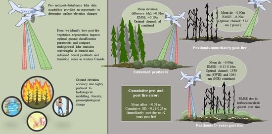
Pre- and post-fire airborne lidar data provide an opportunity to determine peat combustion/loss across broad spatial extents. However, lidar measurements of ground surface elevation are prone to uncertainties. Errors may be introduced in several ways, particularly associated with the timing of data collection and the classification of ground points. Ground elevation data must be accurate and precise when estimating relatively small elevation changes due to combustion and subsequent carbon losses. This study identifies the impact of post-fire vegetation regeneration on ground classification parameterizations for optimal accuracy using TerraScan and LAStools with airborne lidar data collected in three wavelengths: 532 nm, 1064 nm, and 1550 nm in low relief boreal peatland environments. While the focus of the study is on elevation accuracy and losses from fire, the research is also highly pertinent to hydrological modelling, forestry, geomorphological change, etc. The study area includes burned and unburned boreal peatlands south of Fort McMurray, Alberta. Lidar and field validation data were collected in July 2018, following the 2016 Horse River Wildfire. An iterative ground classification analysis was conducted whereby validation points were compared with lidar ground-classified data in five environments: road, unburned, burned with shorter vegetative regeneration (SR), burned with taller vegetative regeneration (TR), and cumulative burned (both SR and TR areas) in each of the three laser emission wavelengths individually, as well as combinations of 1550 nm and 1064 nm and 1550 nm, 1064 nm, and 532 nm. We find an optimal average elevational offset of ~0.00 m in SR areas with a range (RMSE) of ~0.09 m using 532 nm data. Average accuracy remains the same in cumulative burned and TR areas, but RMSE increased to ~0.13 m and ~0.16 m, respectively, using 1550 nm and 1064 nm combined data. Finally, data averages ~0.01 m above the field-measured ground surface in unburned boreal peatland and transition areas (RMSE of ~0.19 m) using all wavelengths combined. We conclude that the ‘best’ offset for depth of burn within boreal peatlands is expected to be ~0.01 m, with single point measurement uncertainties upwards of ~0.25 m (RMSE) in areas of tall, dense vegetation regeneration. The importance of classification parameterization identified in this study also highlights the need for more intelligent adaptative classification routines, which can be used in other environments.

Graphical Abstract

1. Introduction

Boreal peatlands contain considerable carbon (C) stores and have acted as a long-term sink for atmospheric C since the Holocene [1,2]. However, with climate change, many of these peatland regions are drying and becoming more vulnerable to wildland fire [3,4,5], which are increasing in both frequency and severity [4,6]. There is interest in quantifying the contribution of peat combustion to atmospheric C [7,8,9]. Improving estimations of C loss during wildland fire is especially critical in boreal environments, where soil combustion can account for up to ~90% of C loss [7].
In recent years, several studies [6,10,11,12] have described the loss of C from wildland fire in peatlands; however, there are methodological limitations for estimating C loss across a broad range of peatland and boreal ecosystems. Fieldwork is labor-intensive and time-consuming and cannot survey the full range of environmental variations that influence the loss of C from fire in peatland landscapes [8,13,14]. Optical remote sensing is often utilized to estimate burn severity and is particularly useful in its ability to cover broad spatial extents (e.g., [13,15]); however, optical remote sensing of the understory and ground surface is occluded by the pre-fire vegetation canopy and any remaining post-forest canopy—a limitation in assessing burn severity as well as pre-fire conditions [8,13,16]. Therefore, these sensing techniques cannot easily measure ground surface elevation and cannot measure depth of burn, an essential component of biomass loss [9].
Airborne and Unpiloted Aerial Vehicle (UAV) lidar provide an opportunity to resolve both the lack of spatial coverage of field data and reduced ability to determine ground elevation from high spatial resolution optical remote sensing due to occlusion. Lidar is useful for measuring ground surface elevations and vegetation structural characteristics across a range of land cover types, including boreal peatlands (e.g., [17,18,19]). This capability allows for not only the quantification of pre-fire fuels and post-fire ecosystem regeneration in the study of wildland fire (e.g., [9,20,21]), but also in forestry (e.g., [19,22]), urban planning and road design (e.g., [13]), hydrological modelling (e.g., [23]), mapping and modelling of land cover distribution (i.e., wetlands) (e.g., [24,25]), monitoring of permafrost thaw (e.g., [9]), soil erosion (e.g., [26]) and flooding (e.g., [27]). A benefit of the use of lidar is the ability to measure both canopy structure, understory, and ground surface elevation [13]. Multi-temporal, pre- and post-fire lidar data also enable quantification of biomass losses from fire and post-fire vegetation regeneration (e.g., [28]). As laser pulse returns can measure ground surface elevation, the technology is particularly useful for determining surface elevation changes, such as depth of burn during wildland fire, quantification of erosion, and impacts of permafrost slaw if pre- and post-disturbance lidar data are available. However, despite its utility, questions arise on the accuracy of lidar data for determining elevation (and therefore depth of burn, C losses, etc.) associated with different ground classification routines and also, the efficacy of lidar-based observations as time since fire increases. Ref. [13] suggest that most error is introduced during the classification stage; however, custom, environment-specific ground classification parameterization can improve DEM accuracy [19,29]. Due to the need for accurate ground surface data when quantifying relatively small changes in elevation from combustion, erosion, slumping, permafrost thaw, and anthropogenic disturbance, the quantification of ground classification routines specific to land cover and vegetation growth that result in the least error is required. There is also an urgent need for more accurate measurements of soil combustion and overall C losses from boreal peatlands and their potential influence on the global climate system [11,30].
Based on the necessity for accurate ground elevation data for estimating depth of peatland burn in pre- and post-fire lidar data, this study aims to: (a) identify how post-fire vegetation regeneration impacts optimal ground classification configurations using industry-standard software: TerraScan (Terrasolid, Helsinki, Finland) and LAStools (RapidLasso, Gilching, Germany, GmbH); and (b) compare multispectral lidar emission wavelength(s) (532 nm (green); 1064 nm (near infrared); 1550 nm (shortwave infrared); 1064 and 1550 nm combined; and, 532, 1064, and 1550 nm combined) in burned and unburned boreal peatlands and transition zones in western Canada. The overall goal is to provide recommendations for ground classification of lidar data across a range of vegetation regeneration required for quantifying subtle changes in elevation, including depth of burn from fire (in bi-temporal, pre- and post-fire lidar data). While this research focuses on wildland fire, recommendations will also be useful for hydrological modelling, forestry applications, and land surface engineering/mining/cut-fill operations.

2. Materials and Methods

2.1. Study Area

The study area is located about 30 km south of Fort McMurray, Alberta (centre: 12N 482464E 6260554N) in the Boreal Plains ecozone of Canada (Figure 1) [31]. The region is characterized by flat to slightly undulating terrain with some hummocky zones. It is dominated by bog and fen peatlands (dominant wetland classes in Alberta [32]), aspen (Populus tremuloides) uplands, and black spruce (Picea mariana) lowlands/transition zones [31]. Extensive forestry and oil exploration and extraction occur within the region, as do subsistence and commercial hunting and fishing and minor agricultural practices [31].
The study covers a 20,441-ha area south of Fort McMurray, extending beyond the area burned by the Horse River Wildfire in 2016 (Figure 1). The Horse River Wildfire, covering approximately 600,000 ha, ignited 7 km outside Fort McMurray on 1 May 2016, under hazardous conditions—uncharacteristically hot (~35 °C), dry, and windy (~43 km hr−1) weather. The fire was declared under control on 4 July 2016; however, smoldering peat burn continued for approximately 15 months before being extinguished [33,34]. The burned region includes a variety of burn severities and levels of vegetative regeneration since the fire, from little to no regeneration to significant vegetation growth (Figure 2). This allows for the opportunity to compare laser pulse interactions and ground elevation accuracies across a range of conditions akin to timing of lidar data collection following fire.
In sites with shorter regeneration (SR), post-fire vegetation heights averaged 0.20–0.35 m (Figure 2). Dominant vegetation was primarily Sphagnum spp. And feathermoss (Pleurozium spp.), with subdominant vegetation consisting of mosses, herbs, and low-lying herb species such as Labrador tea (Rhododendron groenlandicum), reindeer lichen (Cladonia rangiferina), bog cranberry (Vaccinium oxycoccos), cloudberry (Rubus chamaemorus), and horsetail (Equisetum fluviatile). In sites with taller post-fire vegetative regeneration (TR), above-surface vegetation heights averaged 0.40–1.00 m (Figure 2). While dominant vegetation included some similar species as the SR sites such as feathermoss and Sphagnum spp., sites were also dominated by more woody vegetation and tall shrubs, such as willow (Salix spp.), bog, shrub, and paper birch (Betula pumila, glandulosa, and papyrifera), black spruce (Picea mariana), fireweed (Chamaenerion angustifolium), horsetail (Equisetum spp.), rose (Rosa acicularis), trembling aspen (Populus tremuloides), and raspberry (Rubus idaeus).

2.2. Data Acquisition

Airborne lidar data were collected in July 2018, two years following the Horse River Wildfire, using a Titan multispectral lidar (Teledyne Optech, Inc., Vaughan, ON, Canada). The Titan collects data using three laser emission wavelengths (channels): 1550 nm (shortwave infrared (SWIR); channel 1), which is 3.5° forward of nadir; 1064 nm (near-infrared (NIR); channel 2), which is emitted at nadir; and 532 nm (green; channel 3) which is 7° forward of nadir (Figure 3a) [18]. The survey was flown at ~1000 m above ground, with scan angles of ±25 degrees, a pulse repetition frequency of 100 kHz per channel (300 kHz total), and a 50% flightline overlap. This survey configuration resulted in average point densities of 4.8 pts m-2, 4.2 pts m-2, and 2.1 pts m-2 for channels 1, 2, and 3, respectively. As laser scan lines are not spatially coincident, the 50% overlap reduces gaps, especially prevalent along scan line edges, such that validation points do not exist within one or two channels, introducing bias (Figure 3b).
Field data were collected coincident with the 2018 lidar data collection for the calibration and validation of lidar data. To select sample sites, the study area was first stratified into scales of influence: (a) burned versus non-burned areas within and proximal to the Horse River wildfire; (b) within burned areas, different classes of burn severity (minimum, medium, and severe) determined visually from optical remote sensing imagery as well as through on-the-ground assessments at the time of field data collection; and, (c) peatland type (treed and open bogs; rich and poor fens) determined from optical remote sensing imagery and on-the-ground assessments. Data were collected along ~30 m transects in 18 burned and 6 unburned peatland sites. Transects intersected upland-peatland transition zones and peatlands. Global Navigation Satellite System (GNSS) ground elevation validation points were collected in burned and unburned landscapes. To validate post-fire ground surface elevations [9], GNSS stations were placed at the beginning and end of each transect and were left to run for the duration of sampling (>1 h for centimeter accuracy). Precise Point Positioning (PPP) was used to process these end points. A level was used at one- (burned sites) or two- (unburned sites) meter intervals to determine ground elevation relative to the GNSS base stations. A total of 708 ground elevations were measured: 130 in unburned and 578 in burned peatlands with variable rates of vegetation regeneration. Post Processed Kinematic (PPK) GNSS elevation locations were also collected along two road surfaces (n = 2655) to ensure the elevational accuracy of airborne lidar data in areas of flat terrain without any overstory canopy influences on ground surface elevation [17,35].

2.3. Data Processing

Lidar returns from road surfaces were compared with PPK GNSS survey points and vertically batch-shifted to ensure the average offset between lidar data and calibration points was zero [35] using Bentley Microstation TerraSolid Terrascan software version 021.011 (Terrasolid, Helsinki, Finland) [36]. Isolated or outlier points were removed, and an iterative ground classification analysis was then conducted through which ground vs. non-ground returns were classified. The five ground cover types (road, unburned, short vegetation regeneration (SR), and tall vegetation regeneration (TR), and cumulative burned (all regeneration stages)) were analyzed separately to identify optimal ground return classifications for each type, optimized for relatively flat to slightly undulating boreal peatland and transitional environments with micro-topographic hummocks and hollows.

2.3.1. TerraScan

Within TerraScan, six ground classification parameters can be readily modified: (a) ‘max building size’, which sets the grid size for seed ground point selection; (b) ‘terrain angle’, which is the maximum slope between a seed point and a candidate point; (c) ‘iteration angle’, which is the maximum angle that a point can be added to the ground classification; (d) ‘iteration distance’, which is the maximum distance that a point can be added to the ground classification; (e) ‘reduce iteration angle’, a binary choice which reduces the number of unnecessary points added to the surface in areas of high point density by reducing the number of points that are added to the surface if edge length is longer than all triangle edges; and (f) ‘stop triangulation’, another binary choice which reduces the number of unnecessary points added to the surface by not processing points within a triangle if edge length is longer than all triangle edges [37,38] (Table 1). Adjusting each ground classification parameter results in morphological differences in the resultant ground-classified data.
Thirty-six different ground classification parameterizations were developed by making adjustments to TerraScan’s classification parameters (Table 1). Classifications 1–28 were produced by iterating through adjustments to the four primary parameters: ‘Max Building Size’, ‘Terrain Angle’, ‘Iteration Angle’, and ‘Iteration Distance’. Classifications 29–36 were developed by refining an optimal classification (27) using ‘Reduce Iteration Angle When Edge Length<’ and ‘Stop Triangulation When Edge Length <’ (Table 1). Each of the classification parameterizations was used to produce ground surfaces in the channels and channel combinations tested, resulting in 180 distinct ground surfaces. Each surface output was compared to ground elevation field validation data (elevation collected along the road, unburned peatlands, TR peatlands, SR peatlands, and total burned peatlands) using TerraScan’s control report function (see Section 2.4) for a total of 740 ground classification tests.

2.3.2. LAStools

LASground, from LAStools (RapidLasso GmbH, Gilching, Germany), offers five defined ground classifications that, like TerraScan, use an adaptive TIN algorithm to classify ground points. Two were tested (excluding urban settings): ‘nature’ and ‘wilderness’. These settings differ in their step size (cell size within which lowest point becomes initial ground point) and ‘bulge’ (height allowance for TIN to “bulge” above planar surface). These can be refined using the options ‘default’, ‘fine’, ‘extra’, ‘ultra’, and ‘hyper’, resulting in ten different readily accessible ground classification parameterizations (lettered A–J; Table 2). Using refining options intensifies the search for seed ground points—this is often most useful for ground surfaces with steep hills [39]. Each of the ten different classification parameterizations was used to produce ground surfaces in the channels and channel combinations tested, resulting in 50 distinct ground surfaces. These were brought into TerraScan for the quantification of control point statistics. Like the TerraScan analysis, each ground surface was compared with field elevation measurements from road, unburned peatlands, TR peatlands, SR peatlands, and burned peatlands cumulatively, for a total of 250 ground classification tests.

2.4. Vertical Accuracy Assessment

Ground classification outputs performed using TerraScan (n = 36) and LAStools software (n = 10) in each of the three available laser emission wavelengths and wavelength combinations were compared with field-measured elevations from road (n = 2655), unburned peatlands (n = 130), burned peatlands (n = 578), TR peatlands (n = 267), and SR peatlands (n = 269). Validation data were segregated into TR vs. SR vegetative regeneration based on average measured vegetation height and dominant species per plot (1 m × 1 m with three elevation measures through the center of each plot, perpendicular to the transect; Figure 2). The separation of peatlands based on vegetation provides an opportunity to quantify elevation accuracy from lidar across a range of environmental characteristics, including unburned with a full understory, burned with no or shorter regeneration (SR; a proxy for lidar data collected immediately post-fire), and burned with tall regeneration (TR; a proxy for data collection several years post-fire). Validation data were distributed throughout the study area, and the number of validation elevations measured in the field exceeded the minimum (n = 20) and the recommended (n = 30) suggested for each vegetation cover type by the American Society for Photogrammetry and Remote Sensing [13,40,41]. All ground-classified data were examined in TerraScan, where validation point elevations were compared with lidar point elevations, a standard methodology for lidar vertical accuracy assessments [41,42]. Through TerraScan’s control report function, lidar points were used to interpolate a surface using a Triangulated Irregular Network (TIN). As it is unlikely that a lidar point exists at the same x, y location as a validation point, validation points were compared to their x, y location on the TIN surface [43,44]. Control point statistics, including the difference in elevation between control points and lidar ground returns (dz; average, maximum, and minimum), standard deviation, and root mean square error (RMSE), were quantified via TerraScan’s control report function [44].
To identify the optimal ground classification for each vegetation cover type, classified outputs were assessed based on RMSE (commonly used to determine accuracy) [41,45,46] and by absolute average dz (| d z ¯ |), while also being mindful of point density. Optimal ground classification statistics ( d z ¯ and standard deviation (SD)) were then used to determine total error ( d z ¯ ± SD) when using multitemporal lidar data to assess ground surface elevation changes (pre- and post-fire). The uncertainties associated with multi-temporal surface elevation measurements are independent of one another, so the propagated error (SD) was calculated through quadrature, (Equation (1)), where Q is the average over- or under-estimation of surface elevation change,   a is cumulative SD, d z ¯ b and d z ¯ c   are the average deviations of lidar classified ground surface from the measured ground surface at times b and c, and   b and   c are the SDs of ground surface measurements at two points in time (i.e., pre- and post-fire). Note that the average deviation ( d z ¯ ) is used, and not absolute average deviation (| d z ¯ |).
Q   ±   a = d z ¯ b + d z ¯ c   ± ( b ) 2 + ( c ) 2

3. Results

The results demonstrate wavelength dependencies and optimal ground classification parameterizations for each vegetation cover type tested within TerraScan and LAStools.

3.1. Differences between Ground-Surveyed Road Elevations and Lidar-Measured Road Ground Classifications

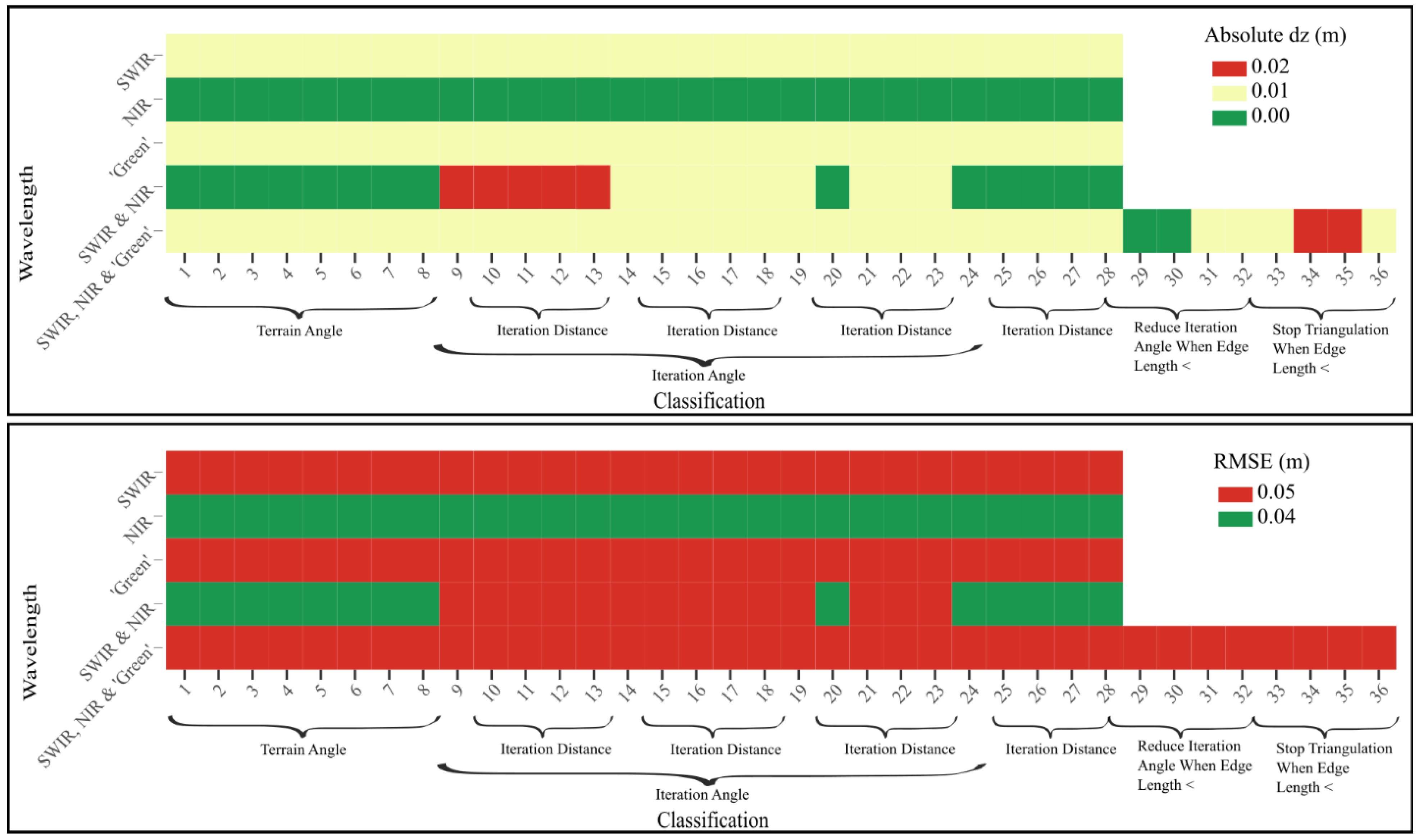
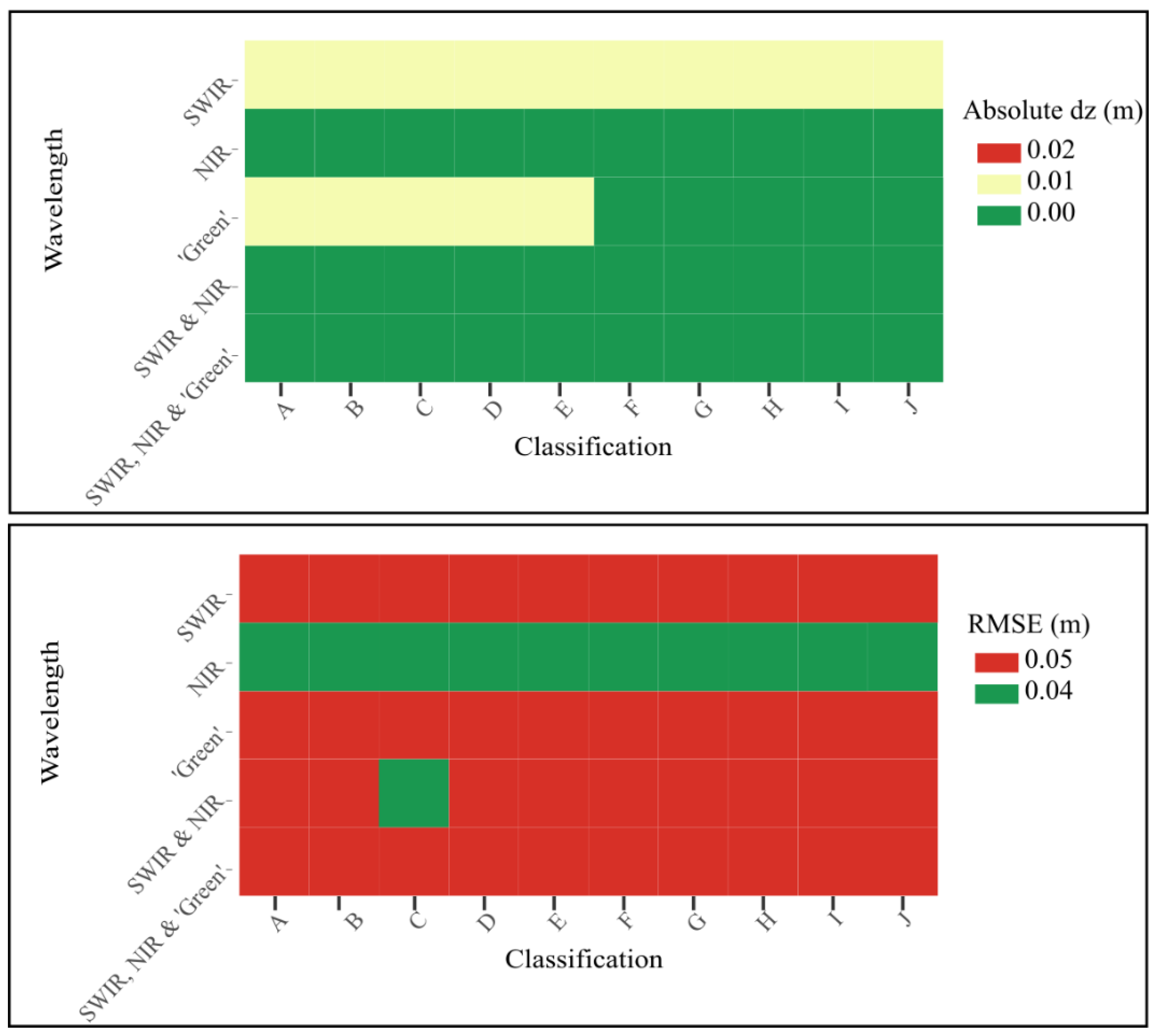
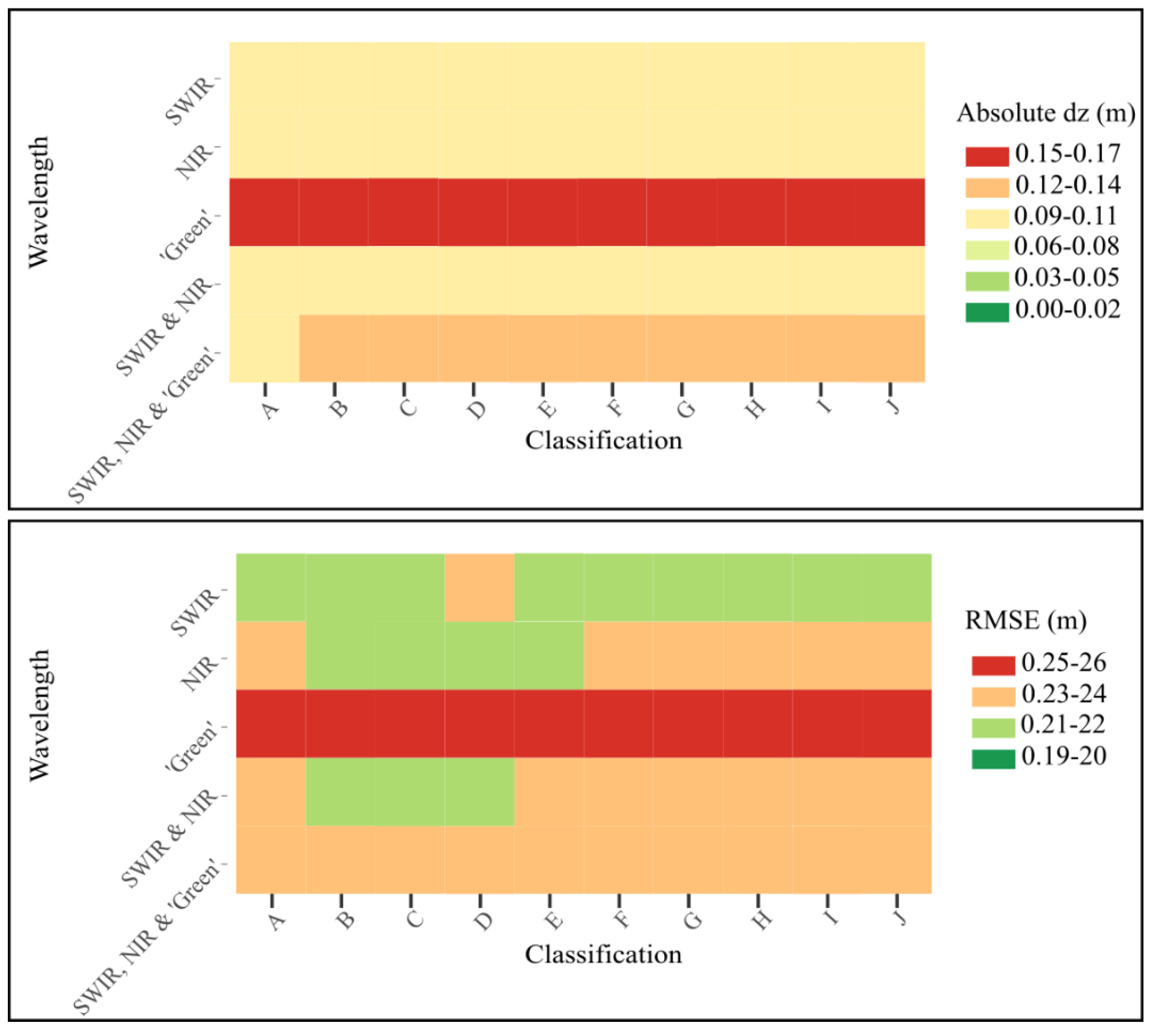
The optimal ground return classification aims to observe the lowest differences in ground surface elevations between field validation and nearby laser returns in each wavelength. Based on the flat, non-vegetated road surface GNSS measurements, we found that neither classification parameter choice (Table 1 and Table 2), nor wavelength, significantly impacted the quality of the ground classification along road surfaces (Figure 4 and Figure 5; Table S1). Using both TerraScan and LAStools, the | d z ¯ | from the measured elevations ranged from 0.00 to 0.02 m, and RMSE from 0.04 m to 0.05 m.
This provides a baseline for comparisons to ground classifications in varying vegetation regeneration stages and demonstrates that any changes observed in ground classification accuracies result from different parameterizations responding differently to variable vegetation regeneration.

3.2. Differences between Field-Measured Elevation and Lidar Return Ground Classification in Shorter Vegetative Regeneration Peatlands

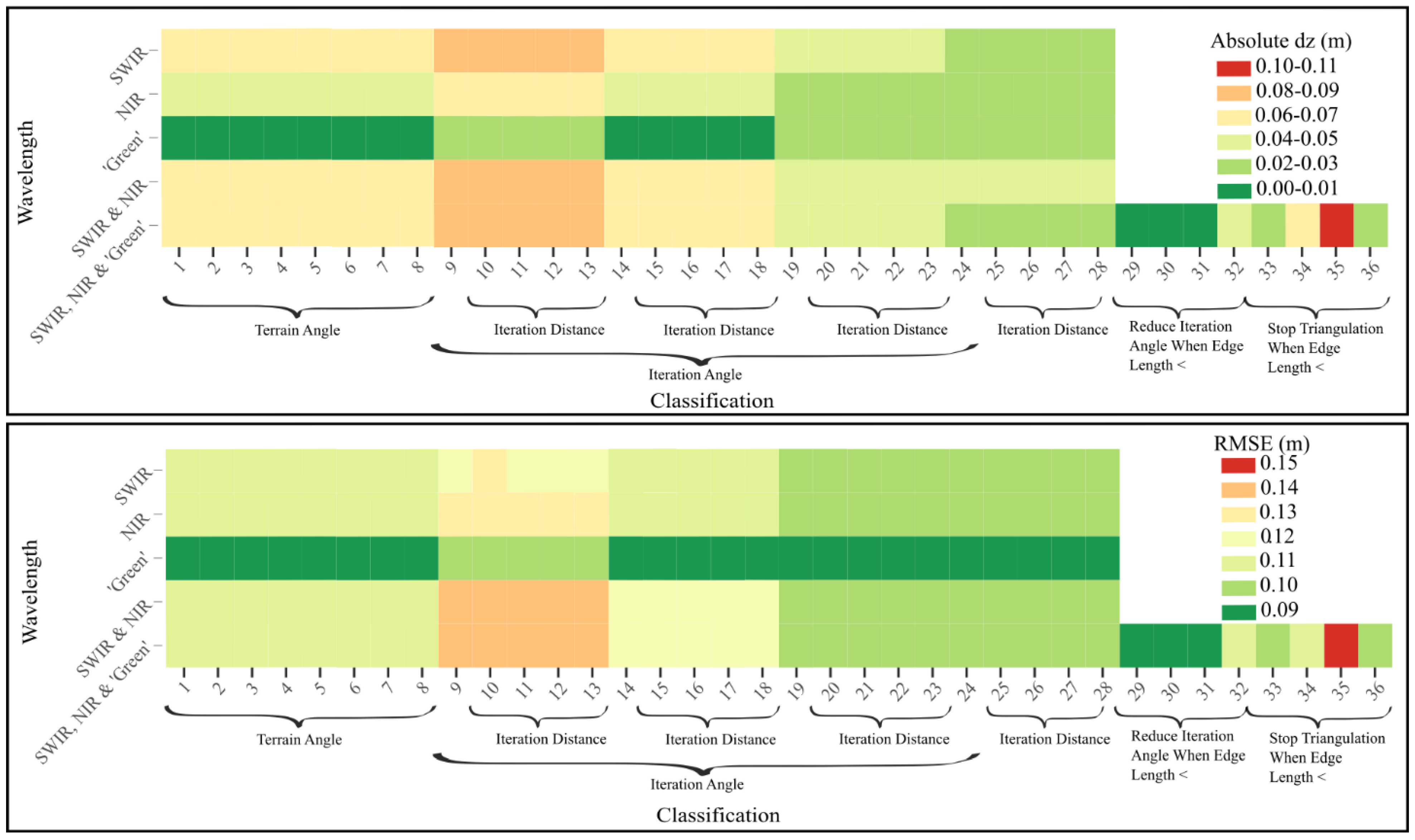
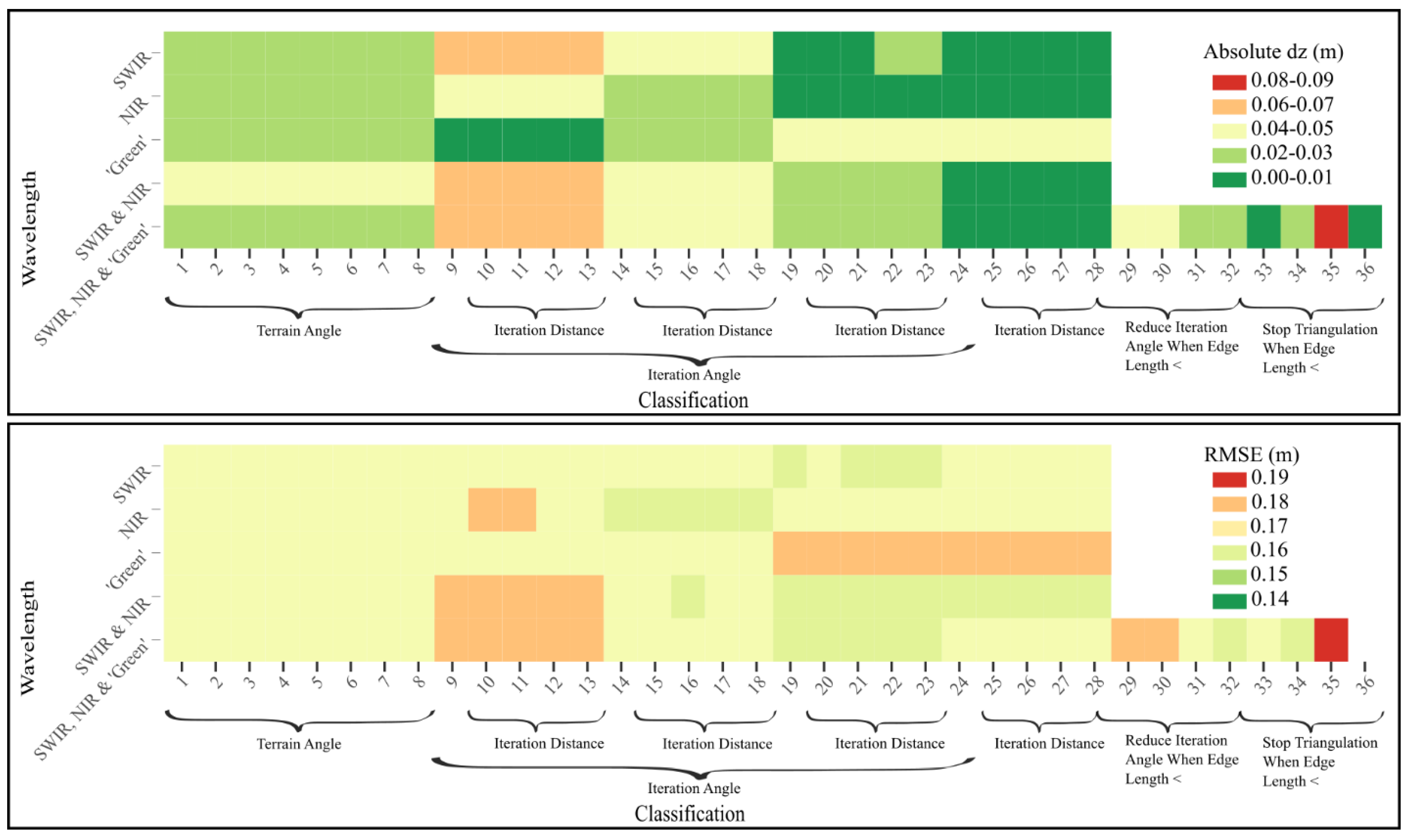
In SR peatlands and transitional areas (representing characteristics that are similar to peatlands that have been surveyed soon after a fire), we found that the ground classifications that produced the most accurate results in TerraScan were classifications 14 through 18 (a slight reduction in iteration angle from six to five as compared to default) with laser pulse emission at 532 nm (Figure 6 and Table 1). These all produced a lidar-derived ground-classified elevation with an | d z ¯ | = 0.00 m (RMSE = 0.09 m). However, the point density was below 1 point m−2; (0.86 points m−2; Table S1). If a higher point density were required, using all three laser pulse emissions (IR, NIR and Visible) and increasing iteration angle from 6 to 15, as well as reducing iteration angle when edge length < 1.0, 2.0, or turned off (classifications 29–31) produce nearly-as-accurate ground surfaces with | d z ¯ | = 0.01 m (RMSE = 0.09 m) and 4.06, 3.94, and 3.32 points m−2, respectively (Figure 6; Table 1 and Table S1). In more typically used lidar systems that collect data at 1064 nm (NIR), the optimal classifications were 24–28 (iteration angle increased from 6 to 15°; Table 1), which resulted in | d z ¯ |s slightly elevated above the true ground surface (| d z ¯ | = 0.03 m; RMSE = 0.10 m; 1.03 points m−2; Figure 6 and Table S1).The poorest ground classifications for SR areas were those within which iteration angle was narrowed to 2°.
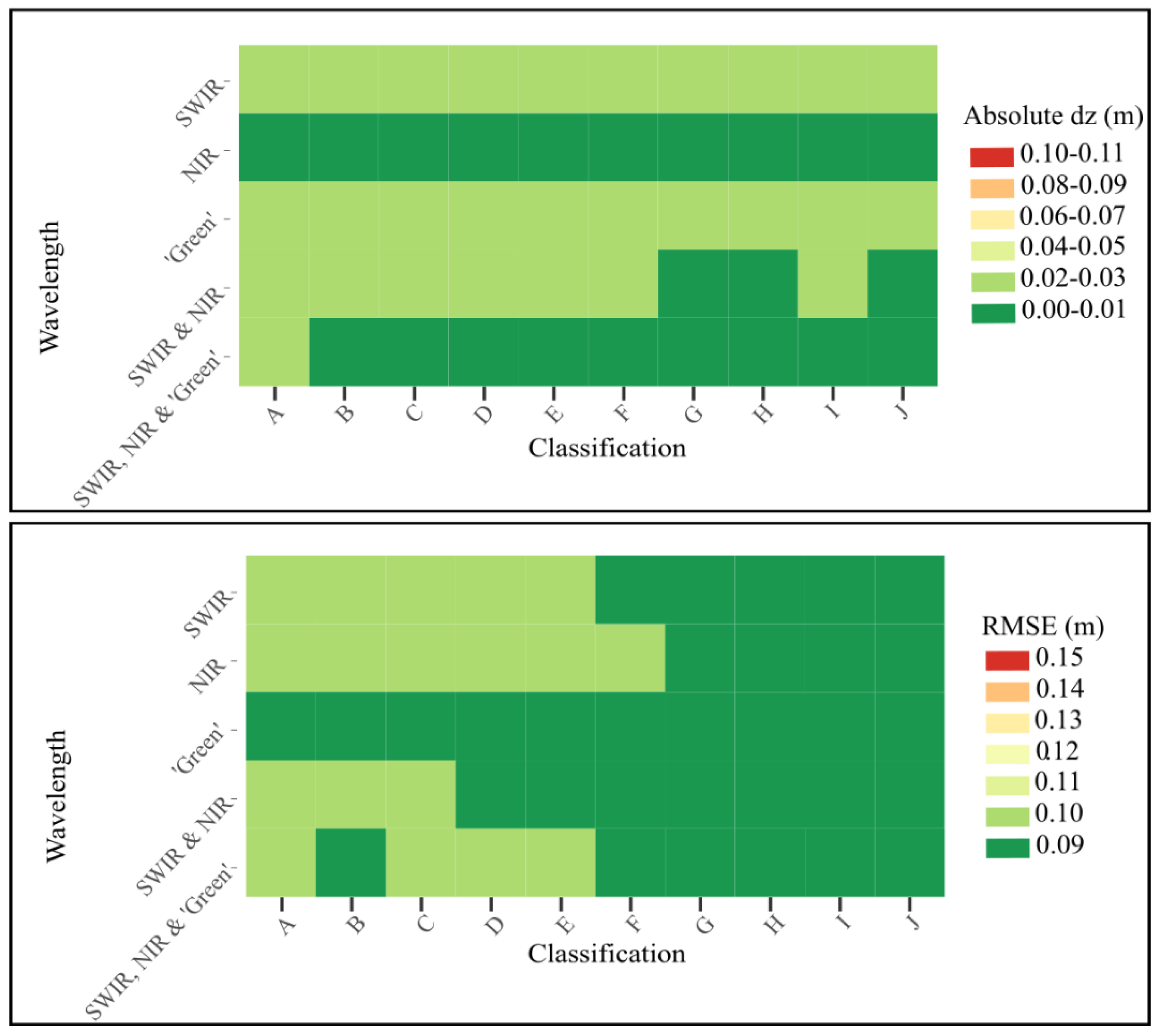
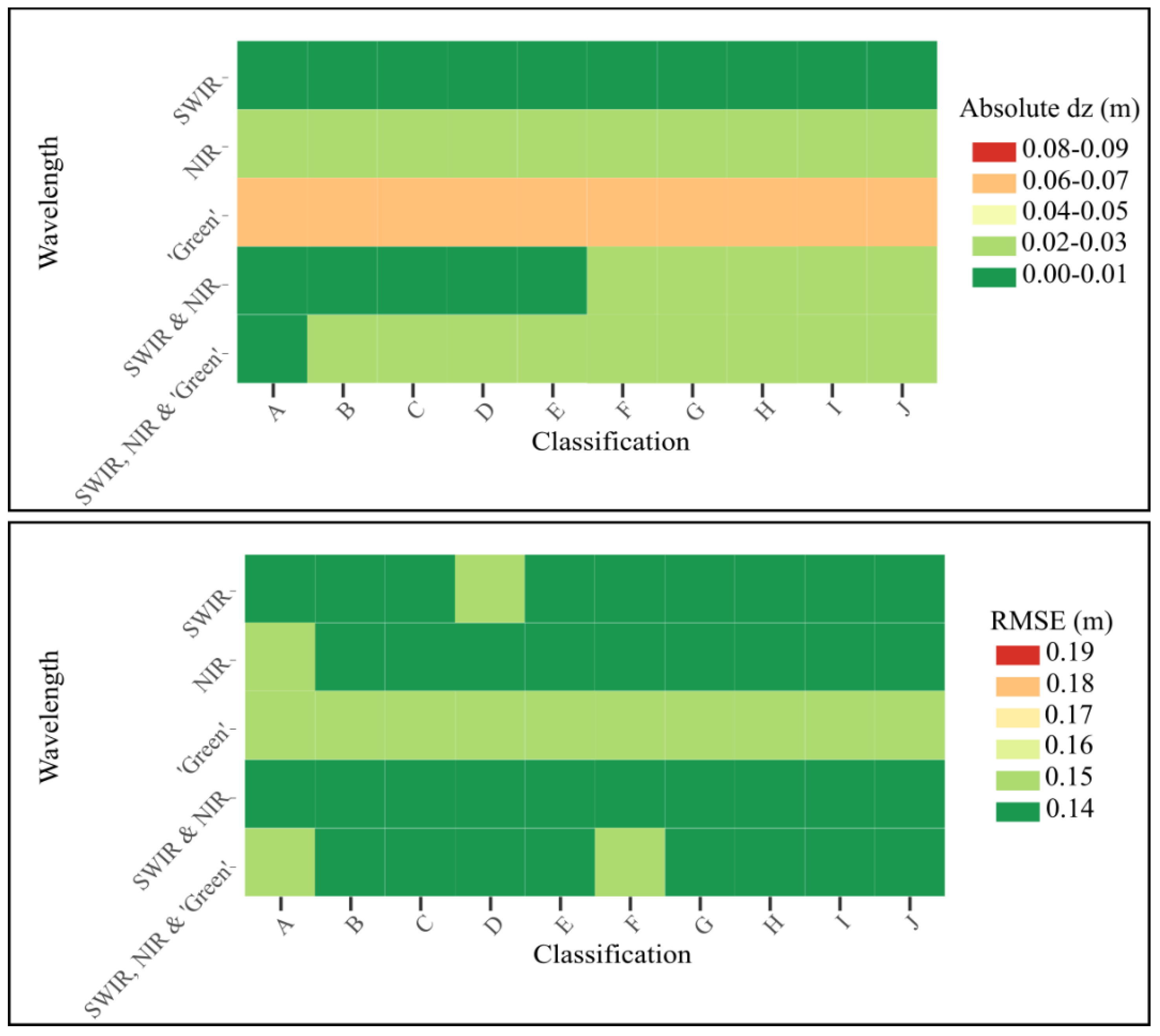
Using LAStools, ground classifications F–J using lidar data collected at all three wavelengths were optimal (Figure 7 and Table 2). These classifications produced lidar-measured ground elevations that did not, on average, deviate from the true ground surface (| d z ¯ | = 0.00 m; RMSE = 0.09 m; 3.70–3.72 points m−2; Figure 7 and Table S1). In this case, where all channels were used, refinement did not impact the ground-classified surface’s accuracy or point density (m−2). In a lidar system that collects data in the 1064 nm wavelength, optimal classifications were G–J, which produced lidar-measured ground classifications with | d z ¯ | = 0.01 m (RMSE = 0.09 m; 1.3–1.31 points m−2; Figure 7 and Table 2). However, in this landscape, when using LAStools, the most significant difference in classification accuracy was due to the channel with which the data were collected; changes within a channel were negligible (i.e., within the 1064 nm data: | d z ¯ | remained at 0.01 m regardless of classification, RMSE only varied by 0.01 m (0.09–0.10 m), and point density varied from 1.24–1.31 points m−2 (Figure 7 and Table S1). While the optimal classifications from TerraScan and LAStools were comparable, the poorest classifications from each were notably different. The classifications produced in LAStools had an | d z ¯ | ranging from 0.00–0.03 m and an RMSE ranging from 0.09–0.10 m, whereas TerraScan classifications had an | d z ¯ | ranging from 0.00–0.09 m and an RMSE ranging from 0.09–0.15 m (Figure 5 and Figure 6).
In summary, for a well-calibrated and locally controlled (e.g., over a nearby highway surface) airborne lidar survey we can expect a spatially averaged difference in elevation of <0.01 m with a range of ~0.09 m in areas of burned ground surface with no to low vegetation regeneration using optimal classifications in both TerraScan and LAStools. However, appropriate parameterization in TerraScan is dependent on the channel(s) available and required point density (Table 1 and Table S1).

3.3. Differences between Field-Measured Elevation and Lidar Ground Classification across All Burned Peatlands (Cumulative Shorter Vegetative Regeneration and Taller Vegetative Regeneration Sites)

As vegetation growth increases in the two years following wildland fire, and vegetation regeneration varies from low (as in SR sites) to high (as in TR sites), optimal ground classification parameters change. In TerraScan, the greatest similarity (and lowest error) when comparing lidar ground-classified returns with the surveyed ground elevation in all burned sites combined (a proxy for ~2 years post-fire) was found when the iteration angle was increased from 6 to 15, but iteration distance was reduced to 0.5 or 1.0 from 1.4 default (parametrization methods 25 or 26) using both 1550 nm and 1064 nm data (Figure 8; Table 1 and Table S1). These classifications produced lidar-measured ground elevations with an | d z ¯ | = 0.00 m (RMSE = 0.13 m; 1.88 points m−2). For a typical 1064 nm laser emission wavelength system, classifications 20 through 23 produced optimal results (iteration angle increased from six to ten), also producing ground elevations with an | d z ¯ | = 0.00 m but with a slightly higher RMSE and lower point density (RMSE = 0.14 m; 1.03 points m−2; Figure 8 and Table 1). As with SR areas, the ground classifications with the lowest accuracy in cumulative burned areas were those whose iteration angle was narrowed to 2.
When compared with optimal ground classification for laser returns in SR landscapes, the optimal ground classification used for total burned areas provides results with comparable | d z ¯ |, but slightly higher uncertainty (SR RMSE = 0.09 m), as would be expected with an increase in vegetation height and height variability.
As in SR areas, classification of returns to ground and elevation accuracy in areas representative of vegetation two years post-fire (cumulative burn areas) depended more on laser pulse emission wavelength than on classification parameters applied in LAStools; however, channel optimization differed. The ground classifications that produced the most accurate results for burned surfaces compared with measured elevations were A through C, E, G, and J (Table 2), using 1550 nm data (| d z ¯ | = 0.00; RMSE = 0.14; point density = 1.27–1.34 points m−2; Figure 9; Table 2); however, within a given wavelength, all parameterizations produced similar results (for example, using 1550 nm data, | d z ¯ | = 0.00–0.01 m; RMSE = 0.14–0.15 m; points m−2 = 1.27–1.34). By using combined 1550 nm and 1064 nm data, similar results are produced (| d z ¯ | = 0.01–0.02 m; RMSE = 0.14) but point density increases to 2.4–2.61 points m−2. Similarly to SR landscapes, optimal classifications from TerraScan and LAStools were negligibly different; however, the poorest classification from LAStools was more accurate than that of TerraScan (| d z ¯ | = 0.06 m; RMSE = 0.15 m and | d z ¯ | = 0.09 m; RMSE = 0.16 m, respectively; Figure 7 and Figure 8).
In the case of more typical 1064 nm lidar systems, classifications B through J produced ground elevations with an | d z ¯ | of 0.02 m, an RMSE of 0.14 m, and 1.24–1.31 points m−2 compared with field-measured; however, even the “poorest” classification (greatest difference from measured) produced from 1064 nm data showed nearly identical results (| d z ¯ | = 0.02; RMSE = 0.15; Figure 9 and Table 2), emphasizing the importance of channel selection during data collection over classification parameterization choice when using LAStools.
In summary, two years post-fire, we can expect an average elevational accuracy of ~0.00 m with a range of ~0.13 m using combined 1550 nm and 1064 nm data with TerraScan. Using LAStools, spatially averaged elevational accuracy is comparable at ~0.00 m but with a slightly higher range of ~0.14 m when measured at 1550 nm.

3.4. Differences between Field-Measured Elevation and Lidar Return Ground Classification in Taller Vegetative Regeneration Peatlands

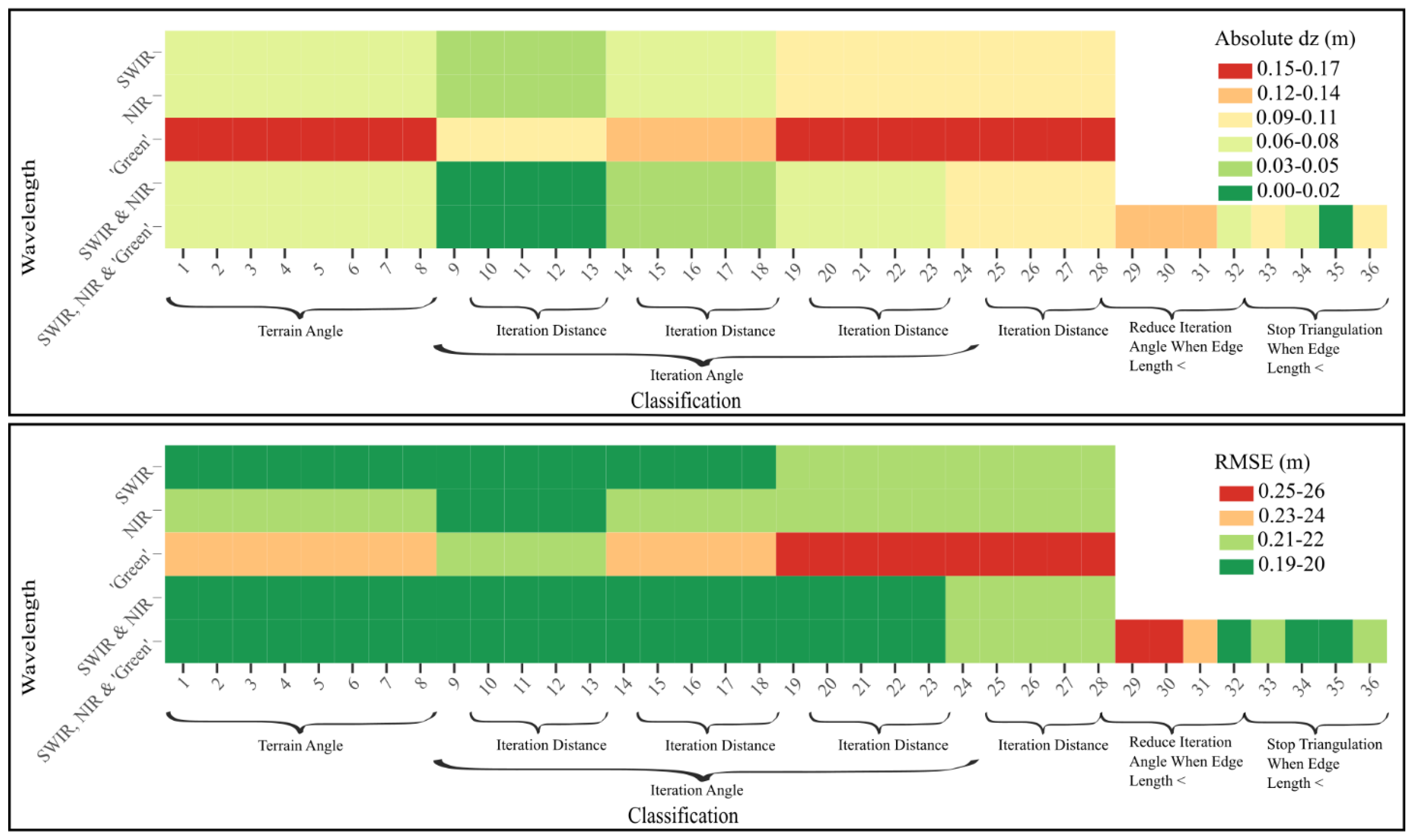
In areas with the greatest vegetation growth since fire (proxies for >2 years post-burn), the most accurate ground classification in TerraScan was classification 20, using combined 1550 nm and 1640 nm data (Figure 10; Table 1 and Table S1). For this classification, the iteration angle was increased from six to ten, and the iteration distance was reduced from 1.4 m to 0.5 m when compared with default parameters. This resulted in a lidar ground classification output with a ground classification accuracy of | d z ¯ | = 0.00 m (RMSE = 0.16 m; 1.54 points m−2). In the case of more typical airborne lidar emitting laser pulses at 1064 nm, this classification still resulted in the most optimal ground surface (with a point density of >1 point m2); however, the lidar-measured ground surface sat ~0.03 m above measured (| d z ¯ | = 0.03 m; RMSE = 0.17 m; 1.03 points m−2). More accurate classification schemes were identified, with fewer (in this case, 0.75) points m−2 (classifications 14 through 18; | d z ¯ | = 0.00 m; RMSE = 0.17 m; Figure 10; Table 1). Generally, the least accurate results were similar to those for cumulative burned areas—those within which the iteration angle was reduced to two; however, in TR areas, emission wavelength made the most difference to accuracy, with the lowest accuracy classifications produced by 532 nm data.
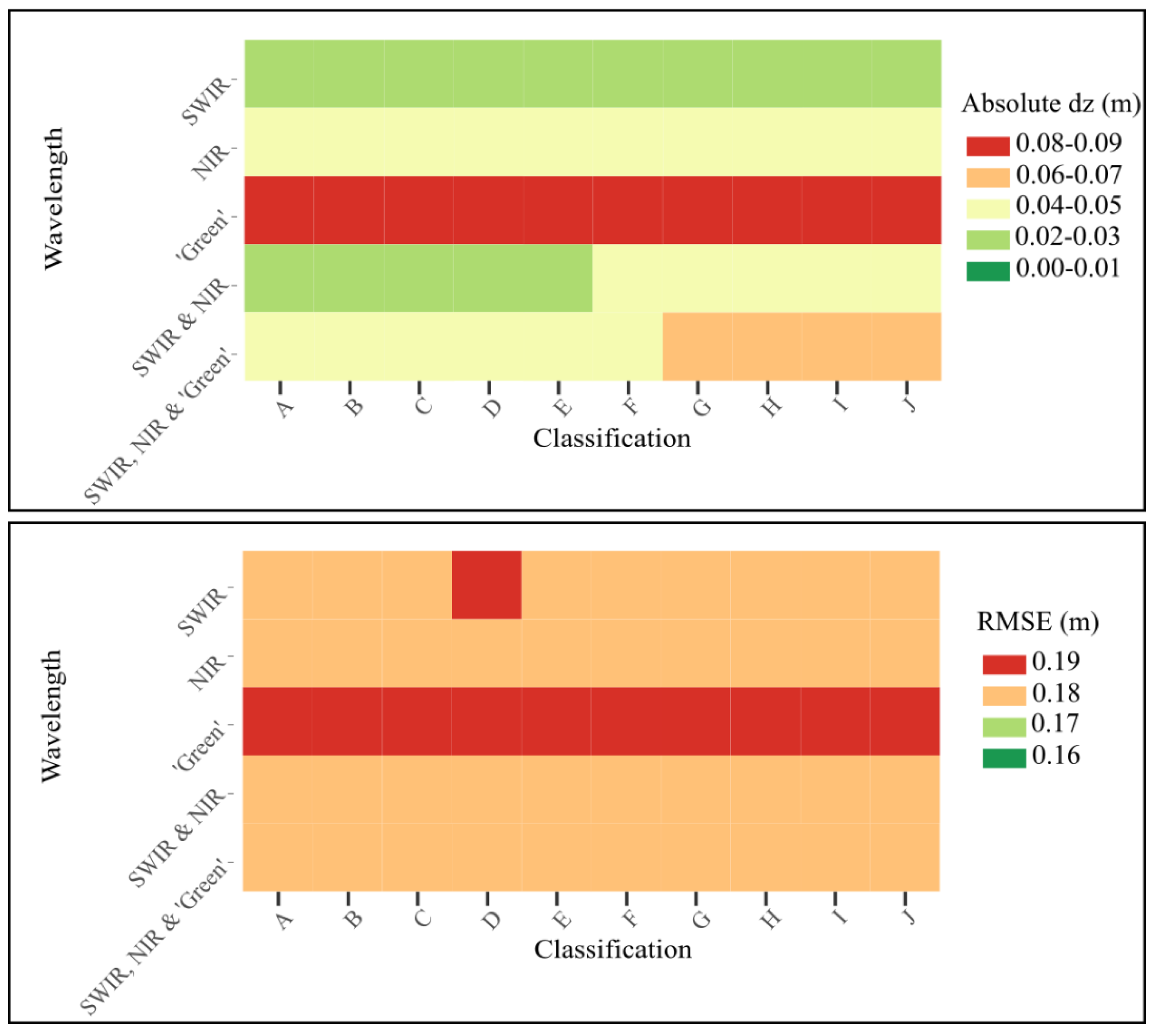
Using LAStools, the optimal ground classifications were A through E (‘Nature’ classifications with any level of refinement) using combined 1550 nm and 1064 nm data (Figure 11; Table 2 and Table S1). The lidar-measured ground classified returns had an | d z ¯ | = 0.03 m from field-measured (RMSE = 0.18 m; 2.40–2.42 points m−2). Comparable results were achieved using only 1550 nm data, but point density was reduced to 1.27–1.34 points m−2. As with earlier vegetation regeneration stages, classification accuracy depended more on the wavelength than on classification parameters with LAStools. For systems using only 1064 nm emission wavelengths, the lidar-measured ground surface sits slightly above the measured ground (| d z ¯ | = 0.04–0.05 m; RMSE = 0.18 m; 1.24–1.31 points m−2). Similar to TerraScan results, the poorest classifications were those produced with 532 nm data.
In summary, unlike areas with lower vegetation regeneration, in TR areas, the optimal classifications from TerraScan and LAStools differed, with TerraScan classifications generally performing better (Figure 10 and Figure 11). Using TerraScan we can still expect an average elevation accuracy of ~0.00 m; however, the accuracy at a given point is expected to have a range of ~0.16 m using combined 1550 nm and 1640 nm data with TerraScan. Using the same lidar data but with LAStools, the average elevational accuracy is slightly lower at ~0.03 m, with a slightly increased RMSE of ~0.18 m.

3.5. Differences between Field-Measured Elevation and Lidar Return Ground Classification in Unburned Peatlands

Finally, in unburned areas (or areas that have fully regenerated post-fire), the optimal ground classifications were 9 through 13 using all wavelengths combined (Figure 12; Table 1 and Table S1). By reducing the iteration angle to two, these classifications resulted in an | d z ¯ | = 0.01 m and an RMSE = 0.19 m; however, point density was relatively low for this particular survey (0.64 points m−2). When a threshold of 1.0 points m−2 is set, the optimal ground classifications shifted to 14 through 18, with their iteration angles set to 5° (Table S1). These classifications have a point density of 1.16 points m−2, but an | d z ¯ | = 0.05 m (Figure 12; Table 1). In the case of a lidar emitting at 1064 nm, the optimal classifications are the same as those when all wavelengths are combined (9 through 13); however, classification accuracies notably decline with a threshold of 1.0 points m−2. Classifications 19 through 23 provide the best outputs, in this case, with an | d z ¯ | = 0.09 m (RMSE = 0.22 m; 1.03 points m−2). The least accurate classifications are those produced using lidar data collected at 532 nm, where the iteration angle is 15 (widest angle tested).
Unlike in burned landscapes, where classification was not the dominant control on accuracy compared with emission wavelength in LAStools, there was a distinction between classifications in unburned areas. In these zones, classification B using data collected at 1064 nm was optimal (Figure 13 and Table 2), resulting in the lowest difference between field-measured and ground classified returns. This classification resulted in an | d z ¯ | = 0.09 m (RMSE = 0.21 m; 1.24 points m−2). As with other vegetation regeneration stages, data collected at 532 nm resulted in the least accurate ground classifications, regardless of parameterization, followed by use of all channels combined.
In summary, as with TR areas, the optimal classifications from TerraScan and LAStools differed in unburned boreal peatlands. We can expect a spatially averaged elevation accuracy of ~0.01 m (or ~0.05 m with a threshold of point density > 1 point m−2) with an accuracy at a given point within an RMSE of ~0.19 m when using all channels combined, processed in TerraScan (Figure 12). Using LAStools, accuracy was poorer, with an average elevation accuracy of ~0.09 m with an RMSE of ~0.21 m at 1064 nm (Figure 13).

3.6. Expected Ground Surface Elevation Accuracies of Lidar Data in the Years following Wildland Fire

By isolating taller versus shorter vegetative regeneration regions and using these as proxies for time since fire, we can estimate the elevation accuracy of lidar data collection in the years following wildland fire. Within the first year since fire (which we assume is the ‘SR’ category), lidar-measured ground elevation accuracies would be expected to be approximately 0.00 ± 0.09 m ( d z ¯ ± standard deviation (SD); Figure 14a and Table S1). For this classification, as well as the others used, below, SD was equal to RMSE. Approximately two years post-fire (at the time of this lidar data collection, assumed to include burned area surveyed–SR and TR), we would expect to see ground elevation accuracy of approximately 0.00 ± 0.13 m (Figure 14a and Table S1). As vegetation growth continues beyond the third year post-fire (‘TR’ category), the elevation accuracy of the lidar-measured ground classified points would be reduced to approximately 0.00 ± 0.16 m (Figure 14a and Table S1). In unburned areas, elevation accuracy would be approximately 0.01 ± 0.19 m (Figure 14a and Table S1).
As the highest uncertainty (SD) was associated with unburned (pre-fire) areas, the RMSEs associated with surface elevation changes were minimally different depending on the stage of post-fire vegetation regeneration (Figure 14b). By using optimal ground classification schemes, the post-fire d z ¯ s were consistently 0.00 m, and pre-fire was ~0.01 m (Figure 4, Figure 5, Figure 6, Figure 7, Figure 8, Figure 9, Figure 10, Figure 11, Figure 12 and Figure 13; Table S1). As such, the standard offset for elevation change was ~0.01 m, on average, regardless of vegetation regeneration. We found that if lidar data were collected immediately post-fire (i.e., SR areas), SD of the elevation change (depth of burn) was 0.21 m (Figure 14b). If data were collected ~ two years post-fire (i.e., cumulative burned areas), SD was 0.23 m (Figure 14b). Furthermore, if lidar data were collected three or more years post-fire (i.e., TR areas), SD was 0.25 m (Figure 14b).

3.7. Wavelength Dependency of Ground Classification Accuracy as Varies by Vegetation Regeneration

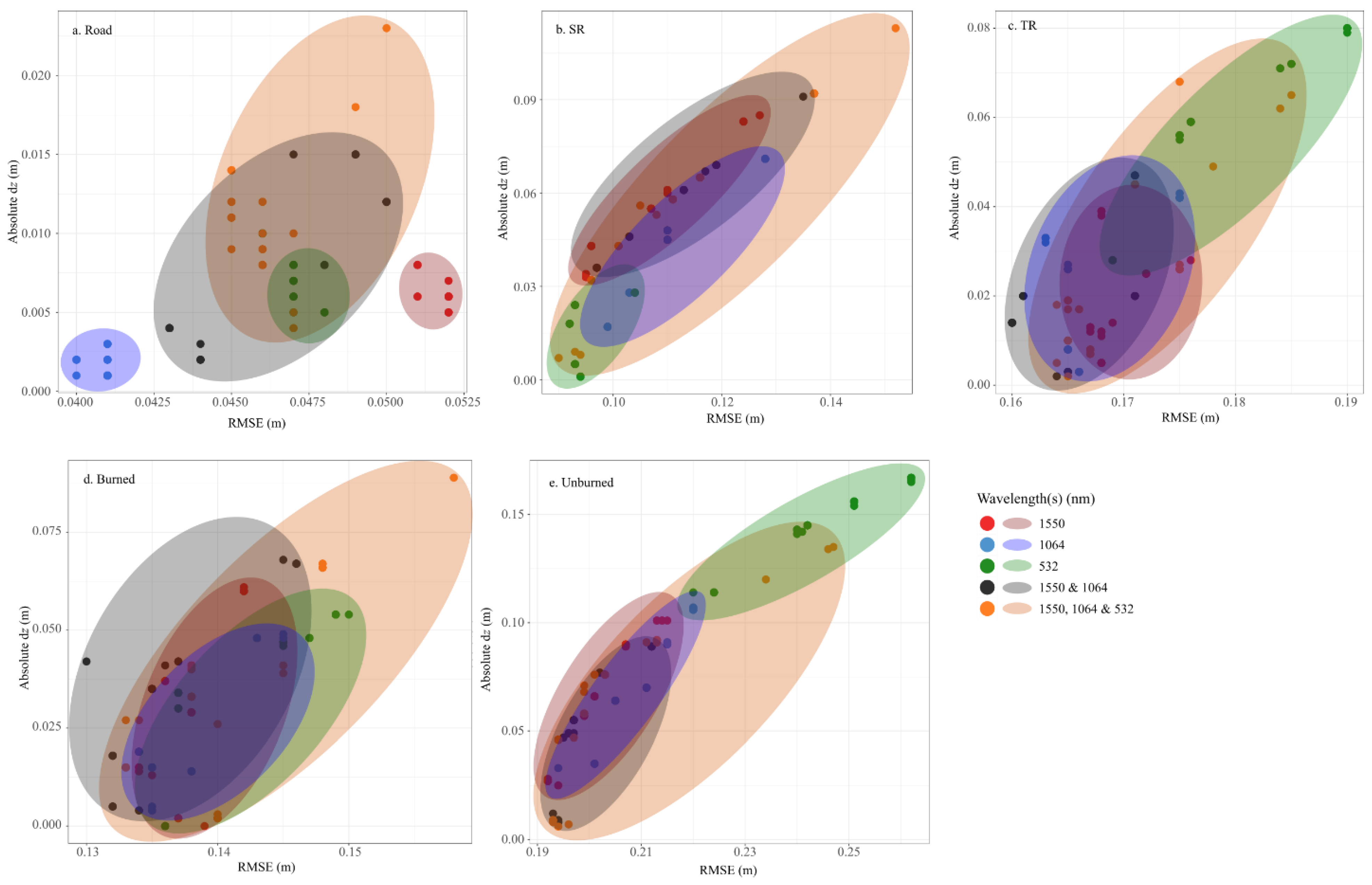
By optimizing parameterizations, highly accurate ground classifications in low relief environments are possible for any wavelength or combination used. However, regardless of processing software, local vegetation characteristics still influence which wavelength produces optimal ground classification results. When applying the TerraScan ground classification parameterizations to road surfaces, optimal ground classification parameterizations derived from 1064 nm data had the lowest error compared with ground control measurements. However, wavelength-associated differences in ground surface elevation were negligible: | d z ¯ |s ranged from 0.00 to 0.02 m (on average for all combination of wavelengths) and RMSEs from 0.04 to 0.05 m (Figure 15a and Table S1). In unburned and TR areas, the combination of 1550 nm and 1064 nm wavelengths resulted in the most accurate ground classifications, with the least variability based on parameterization optimizations (Figure 15e,c). The least wavelength-dependent vegetation regeneration stage was that of cumulative burned areas with variable regeneration heights (a proxy for ~2 years post-fire; Figure 15d). While 1064 nm data resulted in the most accurate ground classifications with the least variability based on the parameterization scheme, the use of any wavelength individually resulted in similar levels of accuracy. However, the accuracy of ground classifications became more variable when wavelengths were combined (either 1550 nm and 1064 nm; or, 1550 nm, 1064 nm, and 532 nm). In SR zones, lidar-based ground elevations measured at 532 nm were the most accurate, with the lowest variability based on parameterizations (Figure 15b).
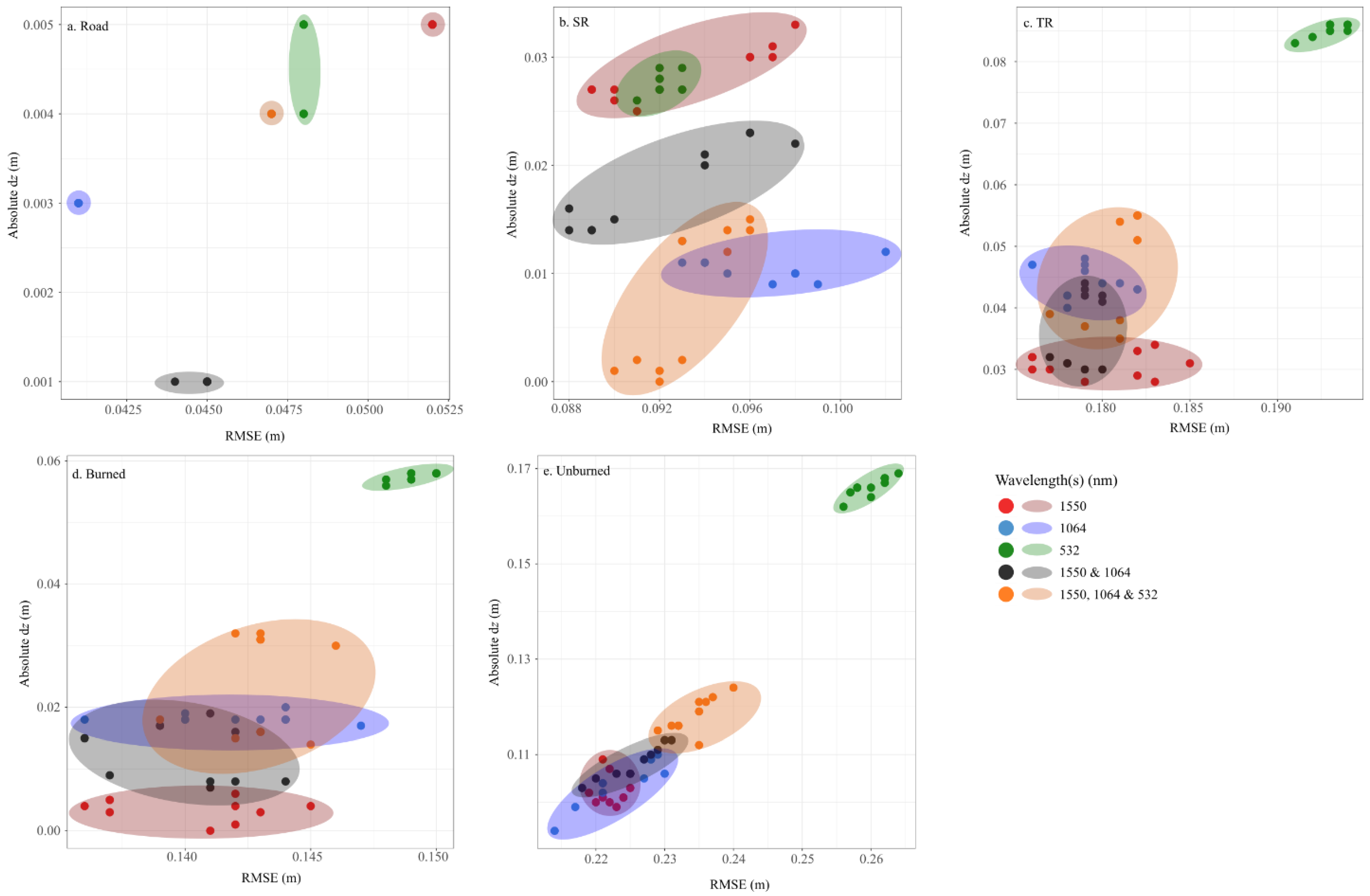
In LAStools, wavelength selection impacted ground classification accuracy more than in TerraScan (Figure 15 and Figure 16). Interestingly, processing software affects wavelength dependency for a given regeneration stage, particularly in SR areas (Figure 15b and Figure 16b). Along road surfaces, the use of data collected at 1064 nm, or both 1550 nm and 1064 nm, resulted in slightly lower RMSEs; however, | d z ¯ | differences were negligible, and RMSEs varied by only ~0.01 m (Figure 16a). In unburned areas, 1064 nm data resulted in ground classifications with the lowest | d z ¯ |s and RMSEs (Figure 16e). Data collected using the 1550 nm wavelength provided the most accurate classifications in both cumulative burned and TR areas (Figure 16d,c). In SR areas, all wavelengths combined provided the most accurate ground classifications (Figure 16b).

4. Discussion

Despite the utility of lidar data for measuring ground surface elevation, time-series lidar data pre- and immediately post-fire is relatively rare but is increasing in availability with the application of lidar for understanding the impacts of wildland fire on ecosystems. This study provides an opportunity to assess the potential for error during the classification of lidar returns as “ground” and the accuracy of ground elevations for use in DEMs. It also identifies the ground classification errors associated with scorched patches/new vegetation regeneration (SR) and early post-fire regeneration stages, indicating time since disturbance.
Previous studies have found that errors in ground classification most often occur as a result of steep terrain [19,41,47] or dense vegetation [19,29,48]. Here, the study area is relatively flat, and so the potential for error that results from sloped terrain is greatly reduced (e.g., [19]). However, where vegetation has regenerated post-fire, stems and foliage can be relatively dense. Further, burned peatland surfaces can have significant microtopographical variability (hummocks and hollows) that may be difficult for the lidar ground classification to differentiate from short, dense vegetation (e.g., [49]). Our results show that within a given vegetation height range, the accuracies of lidar ground classifications (provided the parameters are set logically) do not deviate greatly from the most to least accurate ground classification of laser returns compared with ground control (Table S1). For example, within SR zones, using the least accurate classification scheme/wavelength combination results in classified returns that were, on average, 0.11 m below measured ground elevation, with a RMSE of 0.15 m. For many applicationns, such as canopy height measurements in forested environments, this may be sufficient (e.g., [50]); however, it is important to achieve the best accuracy possible when determining ground surface elevations for applications including combustion from wildland fire (e.g., using pre- and post-fire datasets) and hydrological modelling (e.g., [19]). This is due to the need for accurate quantification of slight differences in the elevation surface from pre-post fire or spatial changes in local surface topography.
We found that as vegetation regenerates post-fire, both optimal parameterizations and the wavelength used for lidar data collection differ at varying growth stages. In SR areas, or immediately post-fire, laser pulse emissions at 532 nm or using all wavelengths combined (532 nm, 1064 nm, and 1550 nm) provide the most accurate ground classifications compared with measured (Figure 4, Figure 5, Figure 15 and Figure 16; Table S1). In these areas where vegetation regeneration was minimal, laser pulses emitted at 532 nm better characterized the ground surface due to the dominance of moss cover in measurement plots with little overlying vegetation in these peatland environments. It should be noted that channel dependencies are likely a result of both wavelength as well as pulse geometry (beam angle and footprint). Pulses emitted at 532 nm have lower energy receipt, a wider footprint, and a tendency to reflect from green vegetation above the ground surface (Figure 3a) [51,52]. As such, ground classified returns at 532 nm were the least accurate in unburned and TR areas (Figure 15 and Figure 16).
As vegetation heights increased, the data from 1064 nm, 1550 nm, or both wavelengths combined, produced the most accurate elevations, noting that the addition of the 532 nm wavelength reduced accuracy even when combined with the other two (Figure 15 and Figure 16). In cumulative burned areas, the use of 1550 nm provided the most optimal ground classifications, while in TR areas, either using 1550 nm data or combined 1064 nm and 1550 nm data had the least error and variability based on parameterizations (Figure 15 and Figure 16). In cumulative burn areas where ground classification was conducted over regions of highly variable vegetation heights and densities, classifications that used 1064 nm data resulted in vegetation misclassified as ground [17,53]. Typical lidar systems with 1064 nm laser wavelength emission have greater reflectance from short vegetation and mosses [54]. Therefore, in areas with low, dense vegetation, there may be energy transmission losses as the laser pulse intercepts and reflects from vegetation instead of the ground surface [9,17,51,53]. This was also observed in [19] who found that low, dense vegetation was more commonly misclassified as ground, such that the classification was less accurate than in areas with tall overstory vegetation and reduced understory, e.g., in some forests. This phenomenon can be seen in the classifications of unburned peatlands, where 1064 nm data were optimal for ground classifications as this resulted in the lowest error (Figure 15 and Figure 16). Here, it is likely that lidar was penetrating through canopies to low-lying understory vegetation (ground dominated by mosses) and the ground surface.
As with channel selection, the parameterization settings that optimized ground classifications depended on the dominant and sub-dominant vegetation heights found within plots. In TerraScan, we found that changes to three parameters impacted ground classifications: iteration angle, iteration distance, and the ability to reduce iteration angle when edge length exceeds a set distance (Table 1 and Table S1). In burned landscapes with little vegetation regeneration (SR), adjustments made to the iteration angle improved the accuracy of the lidar-measured ground elevations compared with field-measured (Table 1 and Table S1). Using 532 nm wavelength data (most accurate but low point density), the iteration angle was slightly reduced from six to five degrees in the optimal classification. Using all wavelengths combined, or only the 1064 nm wavelength data, the iteration angle was increased to 15 and 10 degrees, respectively (Table S1). The classifications using 532 nm data were more optimal using a smaller iteration angle (best for flat landscapes), likely due to the large pulse footprint. However, by increasing the iteration angle when using all wavelengths or 1064 nm data, the classification was better able to retain the steep transitions between hummocks and hollows, which would be most significant in areas with low regeneration, resulting in higher accuracy ground classification. A larger iteration angle allows the ground classification routine to adhere to surface elevation variability [38] by including returns that follow the microtopographic morphology of the hummocks and hollows. Despite the general topography of peatlands and transitions into forests being relatively flat, we are able to optimize the classification to account for highly localized topographic variability by setting the iteration angle to a greater angle within a confined area [10,38].
As vegetation heights increased (cumulative burned and TR areas), maintaining a high iteration angle but reducing iteration distance improved results. Iteration distance, which is the maximum height at which a point will be added to the ground classification [38], may be optimized at a longer distance in landscapes with little vegetation (e.g., for lidar surveys in the months following a fire). This will better account for the discrepancies in dz from returns from hummocks vs. hollows. However, in areas with greater vegetation regeneration and fewer scorched gaps between vegetation patches, a larger iteration distance of 1.4 m (vs. 0.5 m) may result in some returns from short vegetation being included in the ground classification. This increases the lidar ground classified elevation surface above the measured ground surface elevation, thereby increasing the inaccuracy of the DEM (Table 1 and Table S1). Optimal parameterizations change notably in unburned areas or in areas with complete vegetation regeneration, post-fire. Interestingly, the optimal classifications in these regions had a reduced iteration angle of two degrees, which was the iteration angle that resulted in the poorest classifications in all post-burn analyses, even in TR areas. As peat combustion can enhance elevation differences between hummocks and hollows in peatlands [55], unburned peatlands often have less undulating moss ground surfaces. Further, reducing the iteration angle in unburned areas reduces the likelihood of including low herbaceous or shrubby vegetation in the ground classification. However, by reducing the iteration angle, the tendency to add more points into the ground class is also reduced, thereby reducing the point density. We found that by increasing the iteration angle to 5°, point density was increased to >1 point m−2; however, this increased the d z ¯ as the routine included low-lying vegetation as ground.
When using LAStools, we found that classification parameters were less important than the channel (laser pulse emission/reception wavelength as well as pulse geometry) with which data were collected. In SR and TR areas, ground elevation classifications were slightly improved when step size was set to 5 (‘Nature’ setting) instead of 3 (‘Wilderness’ setting) but were not impacted by the level of refinement. The ground classification was slightly better in unburned landscapes when step size was five and refinement was set to ‘Fine’, where the initial ground point search grid is four times more refined than the step size (Table 2 and Table S1).
The results of this study demonstrate that not only do optimal classification parameters differ based on vegetation structures and environmental conditions within these low-relief ecosystems, but also that the same ground classification parameters can be optimal for specific environmental conditions (e.g., burned, low, moderate vegetation regeneration), but far less accurate for a different set of environmental conditions. For example, in TerraScan, classifications 8 through 13 provided the most accurate classifications in unburned landscapes but were the least accurate in cumulative burned and SR areas. There may be more variable ground topography in a burned landscape, which is not optimally parameterized using the same classification. With reduced iteration angle, areas with highly variable microtopography result in underestimation of ground surface elevation because returns from hummocks are excluded from the classification because the angular differences between returns in hollows vs. hummocks is too great. Steep angular classification of returns from the tops of the Sphagnum hummocks resulted in points being added to short vegetation instead of the ground class. This emphasizes the need to classify returns not only by land cover type but also by vegetation characteristics within those land covers for the most optimal/accurate classification parameterization. For example, classification to wetland class, burned and unburned, and within the burned class, high versus low regeneration (which can be determined based on the lidar data derivatives).

5. Conclusions

This study demonstrates the importance of optimizing classification parameters from default settings and optimizing parameters for different land cover types and vegetation structural characteristics. While it is important to iterate/optimize methods with any new data set, the results here provide parameters that can be used in burned and unburned boreal peatland environments and as a starting point for parameterization in similar environments. We provide optimal parameterization for boreal peatlands along a post-fire regeneration trajectory, with “SR” representing peatlands soon after burn, unsegmented burned land cover representing two years post-fire, “TR” representing several years post-fire, and unburned vegetation covers representing land cover later in the regeneration trajectory. However, we suggest that there is a need for the development of accessible adaptative classification procedures, which can be used to (a) filter the landscape by attributes and (b) identify optimal parameterizations.
From this study, we conclude an expected ‘best’ average accuracy for depth of burn (pre-fire elevation minus post-fire elevation) within peatlands will have a spatially averaged error (dz) of ~0.01 m, indicating that soil organic matter loss (determined most simply as a change in elevation) would be over-estimated by an average of 0.01 m. Using the adventitious roots method, the average uncertainty is 0.004 m to 0.04 m (e.g., [54,56,57]) at the tree base. However, airborne lidar methods provide an opportunity to quantify spatially continuous elevational variability between trees and across a broad range of peatlands and environmental characteristics. In addition, we demonstrate that lidar surveys completed in the years following combustion do not become significantly less accurate for quantifying depth of burn overall (offset at ~0.01 m and RMSEs ranging from ~0.21 m to ~0.25 m in SR to TR areas; Figure 14). We suggest that lidar data collected up to three years post-fire can be utilized for depth of burn analyses without significant differences in cumulative errors associated with laser pulse interactions in the understory.

Supplementary Materials

The following supporting information can be downloaded at: https://www.mdpi.com/article/10.3390/rs14205080/s1, Table S1: Ground Classification Results.

Author Contributions

Conceptualization, K.N., L.C. and C.H.; methodology, K.N., L.C. and C.H.; formal analysis, K.N.; investigation, K.N.; resources, L.C. and C.H.; data curation, K.N.; writing—original draft preparation, K.N.; writing—review and editing, K.N., L.C. and C.H.; visualization, K.N.; supervision, L.C.; project administration, L.C.; funding acquisition, L.C., C.H. and K.N. All authors have read and agreed to the published version of the manuscript.

Funding

This research was funded by the Natural Sciences and Engineering Research Council (NSERC) Discovery Grant and University of Lethbridge Start-Up Funding to L. Chasmer. The Teledyne Optech Inc. Titan multispectral lidar was purchased using Western Economic Diversification Canada funding to C. Hopkinson. GNSS equipment was purchased using Canadian Foundation for Innovation funds provided to C. Hopkinson. Research was also funded by post-graduate support of K. Nelson, including the NSERC Canada Graduate Scholarship–Doctoral (CGS D), the Alberta Innovates Graduate Student Scholarship, the Nexen Fellowship in Water Research, and the University Of Lethbridge School Of Graduate Studies, as well as funding from Canada Wildfire (NSERC SPG-N).

Data Availability Statement

Supporting data can be found in Supplementary Information Table S1.

Acknowledgments

The authors would like to thank Linda Flade, Emily Jones, Craig Mahoney, and Maxim Okhrimenko for their field and lidar data collection/processing assistance.

Conflicts of Interest

The authors declare no conflict of interest.

References

  1. Frolking, S.; Roulet, N.T. Holocene radiative forcing impact of northern peatland carbon accumulation and methane emissions. Glob. Change Biol. 2007, 13, 1079–1088. [Google Scholar] [CrossRef]
  2. Yu, Z.C. Northern peatland carbon stocks and dynamics: A review. Biogeosciences 2012, 9, 4071–4085. [Google Scholar] [CrossRef] [Green Version]
  3. Flannigan, M.; Cantin, A.S.; De Groot, W.J.; Wotton, M.; Newbery, A.; Gowman, L.M. Global wildland fire season severity in the 21st century. For. Ecol. Manag. 2013, 294, 54–61. [Google Scholar] [CrossRef]
  4. Miller, C.A.; Benscoter, B.W.; Turetsky, M.R. The effect of long-term drying associated with experimental drainage and road construction on vegetation composition and productivity in boreal fens. Wetl. Ecol. Manag. 2015, 23, 845–854. [Google Scholar] [CrossRef]
  5. Walker, X.J.; Mack, M.C.; Johnstone, J.F. Stable carbon isotope analysis reveals widespread drought stress in boreal black spruce forests. Glob. Change Biol. 2015, 21, 3102–3113. [Google Scholar] [CrossRef]
  6. Kohlenberg, A.J.; Turetsky, M.R.; Thompson, D.K.; Branfireun, B.A.; Mitchell, C.P. Controls on boreal peat combustion and resulting emissions of carbon and mercury. Environ. Res. Lett. 2018, 13, 035005. [Google Scholar] [CrossRef] [Green Version]
  7. Van der Werf, G.R.; Randerson, J.T.; Giglio, L.; Collatz, G.J.; Mu, M.; Kasibhatla, P.S.; Morton, D.C.; DeFries, R.S.; Jin, Y.; van Leeuwen, T.T. Global fire emissions and the contribution of deforestation, savanna, forest, agricultural, and peat fires (1997–2009). Atmos. Chem. Phys. 2010, 10, 11707–11735. [Google Scholar] [CrossRef] [Green Version]
  8. Thompson, D.K.; Waddington, J.M. A Markov chain method for simulating bulk density profiles in boreal peatlands. Geoderma 2014, 232, 123–129. [Google Scholar] [CrossRef]
  9. Chasmer, L.E.; Hopkinson, C.D.; Petrone, R.M.; Sitar, M. Using multitemporal and multispectral airborne lidar to assess depth of peat loss and correspondence with a new active normalized burn ratio for wildfires. Geophys. Res. Lett. 2017, 44, 11851–11859. [Google Scholar] [CrossRef] [Green Version]
  10. Mickler, R.A.; Welch, D.P.; Bailey, A.D. Carbon emissions during wildland fire on a North American temperate peatland. Fire Ecol. 2017, 13, 34–57. [Google Scholar] [CrossRef]
  11. Lin, S.; Liu, Y.; Huang, X. Climate-induced Arctic-boreal peatland fire and carbon loss in the 21st century. Sci. Total Environ. 2021, 796, 148924. [Google Scholar] [CrossRef] [PubMed]
  12. Morison, M.; van Beest, C.; Macrae, M.; Nwaishi, F.; Petrone, R. Deeper burning in a boreal fen peatland 1-year post-wildfire accelerates recovery trajectory of carbon dioxide uptake. Ecohydrology 2021, 14, e2277. [Google Scholar] [CrossRef]
  13. Aguilar, F.J.; Mills, J.P. Accuracy assessment of LiDAR-derived digital elevation models. Photogramm. Rec. 2008, 23, 148–169. [Google Scholar] [CrossRef]
  14. Hokanson, K.J.; Lukenbach, M.C.; Devito, K.J.; Kettridge, N.; Petrone, R.M.; Waddington, J.M. Groundwater connectivity controls peat burn severity in the boreal plains: Groundwater controls peat burn severity. Ecohydrology 2016, 9, 574–584. [Google Scholar] [CrossRef]
  15. Whitman, E.; Parisien, M.A.; Holsinger, L.M.; Park, J.; Parks, S.A. A method for creating a burn severity atlas: An example from Alberta, Canada. Int. J. Wildland Fire 2020, 29, 995–1008. [Google Scholar] [CrossRef]
  16. Hudak, A.T.; Morgan, P.; Bobbitt, M.J.; Smith AM, S.; Lewis, S.A.; Lentile, L.B.; Robichaud, P.R.; Clark, J.T.; McKinley, R.A. The relationship of multispectral satellite imagery to immediate fire effects. Fire Ecol. 2007, 3, 64–90. [Google Scholar] [CrossRef]
  17. Hopkinson, C.; Chasmer, L.; Sass, G.; Creed, I.; Sitar, M.; Kalbfleisch, W.; Treitz, P. Vegetation class dependent errors in lidar ground elevation and canopy height estimates in a boreal wetland environment. Can. J. Remote Sens. 2005, 31, 191–206. [Google Scholar] [CrossRef]
  18. Ekhtari, N.; Glennie, C.; Fernandez-Diaz, J.C. Classification of airborne multispectral lidar point clouds for land cover mapping. IEEE J. Sel. Top. Appl. Earth Obs. Remote Sens. 2018, 11, 2068–2078. [Google Scholar] [CrossRef]
  19. Moudrý, V.; Klápště, P.; Fogl, M.; Gdulová, K.; Barták, V.; Urban, R. Assessment of LiDAR ground filtering algorithms for determining ground surface of non-natural terrain overgrown with forest and steppe vegetation. Measurement 2020, 150, 107047. [Google Scholar] [CrossRef]
  20. Andersen, H.E.; McGaughey, R.J.; Reutebuch, S.E. Estimating forest canopy fuel parameters using LIDAR data. Remote Sens. Environ. 2005, 94, 441–449. [Google Scholar] [CrossRef]
  21. McCarley, T.R.; Hudak, A.T.; Sparks, A.M.; Vaillant, N.M.; Meddens, A.J.; Trader, L.; Francisco, M.; Kreitler, J.; Boschetti, L. Estimating wildfire fuel consumption with multitemporal airborne laser scanning data and demonstrating linkage with MODIS-derived fire radiative energy. Remote Sens. Environ. 2020, 251, 112114. [Google Scholar] [CrossRef]
  22. Chen, Y.; Zhu, X.; Yebra, S.; Harris, N. Development of a predictive model for estimating forest surface fuel load in Australian eucalypt forests with LiDAR data. Environ. Model. Softw. 2017, 97, 61–71. [Google Scholar] [CrossRef]
  23. O’Neil, G.L.; Saby, L.; Band, L.E.; Goodall, J.L. Effects of LiDAR DEM smoothing and conditioning techniques on a topography-based wetland identification model. Water Resour. Res. 2019, 55, 4343–4363. [Google Scholar] [CrossRef]
  24. Millard, K.; Richardson, M. Wetland mapping with LiDAR derivatives, SAR polarimetric decompositions, and LiDAR–SAR fusion using a random forest classifier. Can. J. Remote Sens. 2013, 39, 290–307. [Google Scholar] [CrossRef]
  25. O’Neil, G.L.; Goodall, J.L.; Watson, L.T. Evaluating the potential for site-specific modification of LiDAR DEM derivatives to improve environmental planning-scale wetland identification using Random Forest classification. J. Hydrol. 2018, 559, 192–208. [Google Scholar] [CrossRef]
  26. Neugirg, F.; Kaiser, A.; Schmidt, J.; Becht, M.; Haas, F. Quantification, analysis and modelling of soil erosion on steep slopes using LiDAR and UAV photographs. Proc. Int. Assoc. Hydrol. Sci. 2015, 367, 51–58. [Google Scholar] [CrossRef] [Green Version]
  27. Escobar Villanueva, J.R.; Iglesias Martínez, L.; Pérez Montiel, J.I. DEM generation from fixed-wing UAV imaging and LiDAR-derived ground control points for flood estimations. Sensors 2019, 19, 3205. [Google Scholar] [CrossRef] [PubMed] [Green Version]
  28. Campbell, M.J.; Dennison, P.E.; Kerr, K.L.; Brewer, S.C.; Anderegg, W.R. Scaled biomass estimation in woodland ecosystems: Testing the individual and combined capacities of satellite multispectral and lidar data. Remote Sens. Environ. 2021, 262, 112511. [Google Scholar] [CrossRef]
  29. Schmid, K.A.; Hadley, B.C.; Wijekoon, N. Vertical accuracy and use of topographic LIDAR data in coastal marshes. J. Coast. Res. 2011, 27, 116–132. [Google Scholar] [CrossRef]
  30. Nelson, K.; Thompson, D.; Hopkinson, C.; Petrone, R.; Chasmer, L. Peatland-fire interactions: A review of wildland fire feedbacks and interactions in Canadian boreal peatlands. Sci. Total Environ. 2021, 769, 145212. [Google Scholar] [CrossRef]
  31. Downing, D.J.; Pettapiece, W.W. Natural Regions and Subregions of Alberta; Pub. No. T/852; Government of Alberta Publish: Edmonton, AB, Canada, 2006; 264p.
  32. Alberta Environment and Sustainable Resource Development (ESRD). Alberta Wetland Classification System; Water Policy Branch, Policy and Planning Division: Edmonton, AB, Canada, 2015. [Google Scholar]
  33. MNP LLP. A Review of the 2016 Horse River Wildfire; Forestry Division, Alberta Agriculture and Forestry: Edmonton, AB, Canada, 2017; Available online: https://www.alberta.ca/assets/documents/Wildfire-MNP-Report.pdf (accessed on 20 July 2021).
  34. Institute for Catastrophic Loss Reduction. Fort McMurray Wildfire: Learning from Canada’s Costliest Disaster; Institute for Catastrophic Loss Reduction: Toronto, ON, Canada, 2019; p. 9. Available online: https://www.zurichcanada.com/-/media/project/zwp/canada/docs/english/weather/fort-mcmurray-report_canada.pdf (accessed on 16 May 2021).
  35. Csanyi, N.; Toth, C.K. Improvement of lidar data accuracy using lidar-specific ground targets. Photogramm. Eng. Remote Sens. 2007, 73, 385–396. [Google Scholar] [CrossRef] [Green Version]
  36. Axelsson, P. DEM generation from laser scanner data using adaptive TIN models. Int. Arch. Photogramm. Remote Sens. 2000, 33, 110–117. [Google Scholar]
  37. GeoCue Group. TerraScan Ground Parameters. 2020. Available online: https://support.geocue.com/terrascan-ground-filter-parameters/ (accessed on 10 February 2021).
  38. Terrasolid Ltd. TerraScan User Guide. Terrasolid Ltd., Batch Processing Reference > Classification Routines > Points > Ground. 2021. Available online: https://terrasolid.com/guides/tscan/crground.html (accessed on 10 November 2021).
  39. Rapidlasso GmbH. Lasground_New README. 2021. Available online: https://lastools.github.io/download/lasground_new_README.txt (accessed on 5 December 2021).
  40. ASPRS. ASPRS Guidelines: Vertical Accuracy Reporting for Lidar Data Version 1.0; American Society for Photogrammetry and Remote Sensing Lidar Committee (PAD): Baton Rouge, LA, USA, 2004. [Google Scholar]
  41. Pourali, S.; Arrowsmith, C.; Chrisman, N.; Matkan, A. Vertical accuracy assessment of LiDAR ground points using minimum distance approach. In Proceedings of the Research Locate 14, Canberra, Australia, 7–9 April 2014. [Google Scholar]
  42. Maune, D.; Black, T.; Constance, E. DEM user requirements. In Digital Elevation Model Technologies and Applications: The DEM Users Manual, 2nd ed.; American Society for Photogrammatry and Remote Sensing: Bethesda, MD, USA, 2007; pp. 449–473. [Google Scholar]
  43. Goulden, T.; Hopkinson, C.; Jamieson, R.; Sterling, S. Sensitivity of DEM, slope, aspect and watershed attributes to LiDAR measurement uncertainty. Remote Sens. Environ. 2016, 179, 23–35. [Google Scholar] [CrossRef]
  44. GeoCue Group. Control Point Statistics in TerraScan: TerraScan, Versions 002.001 and Above. 2017. Available online: https://support.geocue.com/wp-content/uploads/2017/03/Control-Point-Statistics-in-TerraScan.pdf (accessed on 10 February 2021).
  45. Carlisle, B.H. Modelling the spatial distribution of DEM error. Trans. GIS 2005, 9, 521–540. [Google Scholar] [CrossRef]
  46. Goulden, T.; Hopkinson, C. The forward propagation of integrated system component errors within airborne lidar data. Photogramm. Eng. Remote Sens. 2010, 76, 589–601. [Google Scholar] [CrossRef]
  47. Goulden, T.; Hopkinson, C. Mapping simulated error due to terrain slope in airborne lidar observations. Int. J. Remote Sens. 2014, 35, 7099–7117. [Google Scholar] [CrossRef]
  48. Hopkinson, C.; Chasmer, L.E.; Zsigovics, G.; Creed, I.F.; Sitar, M.; Treitz, P.; Maher, R.V. Errors in LIDAR ground elevations and wetland vegetation height estimates. Int. Arch. Photogramm. Remote Sens. Spat. Inf. Sci. 2004, 36, 108–113. [Google Scholar]
  49. Brubaker, K.M.; Myers, W.L.; Drohan, P.J.; Miller, D.A.; Boyer, E.W. The use of LiDAR terrain data in characterizing surface roughness and microtopography. Appl. Environ. Soil Sci. 2013, 2013, 891534. [Google Scholar] [CrossRef]
  50. Tinkham, W.T.; Smith, A.M.; Hoffman, C.; Hudak, A.T.; Falkowski, M.J.; Swanson, M.E.; Gessler, P.E. Investigating the influence of LiDAR ground surface errors on the utility of derived forest inventories. Can. J. For. Res. 2012, 42, 413–422. [Google Scholar] [CrossRef]
  51. Hopkinson, C.; Chasmer, L.; Gynan, C.; Mahoney, C.; Sitar, M. Multisensor and multispectral lidar characterization and classification of a forest environment. Can. J. Remote Sens. 2016, 42, 501–520. [Google Scholar] [CrossRef]
  52. Okhrimenko, M.; Coburn, C.; Hopkinson, C. Multispectral lidar: Radiometric calibration, canopy spectral reflectance, and vegetation vertical SVI profiles. Remote Sens. 2019, 11, 1556. [Google Scholar] [CrossRef] [Green Version]
  53. Reddy, A.D.; Hawbaker, T.J.; Wurster, F.; Zhu, Z.; Ward, S.; Newcomb, D.; Murray, R. Quantifying soil carbon loss and uncertainty from peatland wildfire using multi-temporal LiDAR. Remote Sens. Environ. 2015, 170, 306–316. [Google Scholar] [CrossRef]
  54. Gerrand, S.; Aspinall, J.; Jensen, T.; Hopkinson, C.; Collingwood, A.; Chasmer, L. Partitioning carbon losses from fire combustion in a montane valley, Alberta Canada. For. Ecol. Manag. 2021, 496, 119435. [Google Scholar] [CrossRef]
  55. Benscoter, B.W.; Greenacre, D.; Turetsky, M.R. Wildland fire as a key determinant of peatland microtopography. Can. J. For. Res. 2015, 45, 1132–1136. [Google Scholar] [CrossRef]
  56. Kasischke, E.S.; Johnstone, J.F. Variation in postfire organic layer thickness in a black spruce forest complex in interior Alaska and its effects on soil temperature and moisture. Can. J. For. Res. 2005, 35, 2164–2177. [Google Scholar] [CrossRef] [Green Version]
  57. Boby, L.A.; Schuur, E.A.; Mack, M.C.; Verbyla, D.; Johnstone, J.F. Quantifying fire severity, carbon, and nitrogen emissions in Alaska’s boreal forest. Ecol. Appl. 2010, 20, 1633–1647. [Google Scholar] [CrossRef]
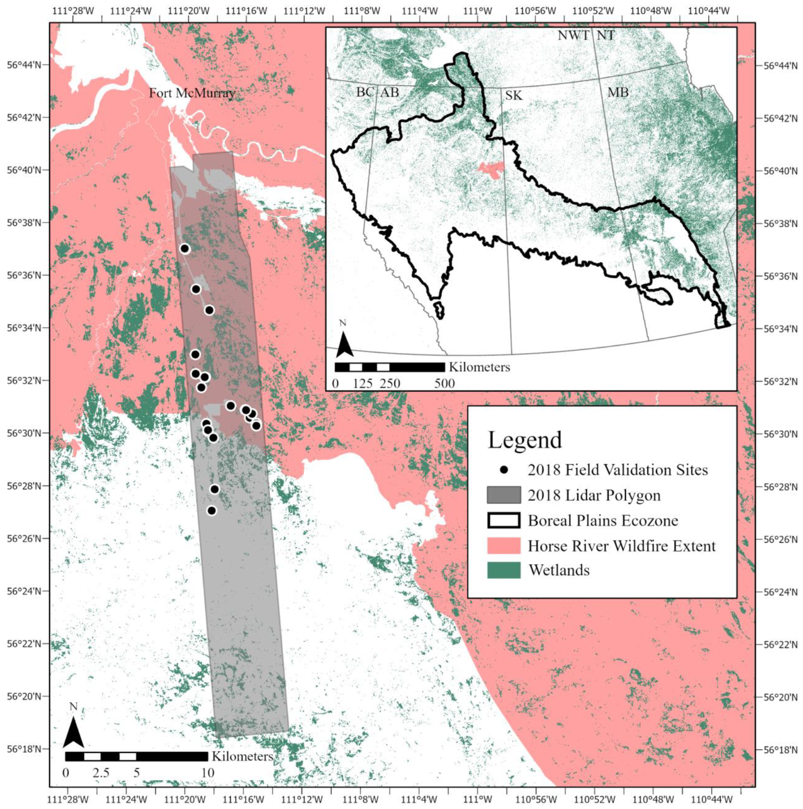
Figure 1. Map illustrating the extent of the Horse River Wildfire within the Boreal Plains Ecozone (inset), which extends across Canada from northern British Columbia (BC) and into Alberta (AB), Saskatchewan (SK), and Manitoba (MB) and the study area, including lidar survey polygon and field validation transects/plots.
Remotesensing 14 05080 g001
Figure 2. Four vegetation categories used to represent time since fire with field photos and lidar point clouds.
Remotesensing 14 05080 g002
Figure 3. (a) Illustration of lidar laser beam angles, beam divergence, and impact on footprint diameter (Ø) in peatlands with variable microtopography (hollows and hummocks); (b) Samples of validation transects and lidar data demonstrating spatial distribution of validation points throughout the three channels. Note: microtopography in (a) has been exaggerated for demonstration purposes.
Remotesensing 14 05080 g003
Figure 4. Ground classification results (| d z ¯ | and RMSE) along a flat road surface for baseline comparisons using parameterization methods in Table 1. Classifications were conducted in TerraScan.
Remotesensing 14 05080 g004
Figure 5. Ground classification results (| d z ¯ | and RMSE) along a flat road surface for baseline comparisons using parameterization methods in Table 2. Classifications were conducted in LAStools.
Remotesensing 14 05080 g005
Figure 6. Ground classification results (| d z ¯ | and RMSE) in burned peatlands with low vegetation regeneration two years post-fire (as a proxy for immediately post-fire). Classifications were conducted in TerraScan.
Remotesensing 14 05080 g006
Figure 7. Ground classification results (| d z ¯ | and RMSE) in burned peatlands with low vegetation regeneration two years post-fire (as a proxy for immediately post-fire). Classifications were conducted in LAStools.
Remotesensing 14 05080 g007
Figure 8. Ground classification results (| d z ¯ | and RMSE) in burned peatlands unsegregated based on vegetation regeneration two years post-fire (true representation of two years post-fire). Classifications were conducted in TerraScan.
Remotesensing 14 05080 g008
Figure 9. Ground classification results (| d z ¯ | and RMSE) in burned peatlands unsegregated based on vegetation regeneration two years post-fire (true representation of two years post-fire). Classifications were conducted in LASTools.
Remotesensing 14 05080 g009
Figure 10. Ground classification results (| d z ¯ | and RMSE) in burned peatlands with tall vegetation regeneration two years post-fire (as a proxy for 3+ years post-fire). Classifications were conducted in TerraScan.
Remotesensing 14 05080 g010
Figure 11. Ground classification results (| d z ¯ | and RMSE) in burned peatlands with tall vegetation regeneration two years post-fire (as a proxy for 3+ years post-fire). Classifications were conducted in LAStools.
Remotesensing 14 05080 g011
Figure 12. Ground classification results (| d z ¯ | and RMSE) in unburned peatlands. Classifications were conducted in TerraScan.
Remotesensing 14 05080 g012
Figure 13. Ground classification results (| d z ¯ | and RMSE) in unburned peatlands. Classifications were conducted in LAStools.
Remotesensing 14 05080 g013
Figure 14. (a) Expected ground elevation accuracies of lidar data in the years following wildland fire in boreal peatlands; (b) Expected depth of burn (DOB) accuracies of lidar data in the years following wildland fire in boreal peatlands, assuming pre-fire lidar data were collected in “unburned conditions”, where Q = average over- or under-estimation of surface elevation change, and Ea is cumulative error (SD). Note: for all measurements used, SD was equal to RMSE.
Remotesensing 14 05080 g014
Figure 15. Ground classification results by wavelength along/in: (a) roads, (b) burned peatlands with short regeneration, (c) burned peatlands with tall regeneration, (d) all burned peatlands, and (e) unburned peatlands two years post-fire. Results were identified using TerraScan as determined by lidar channel. Each point represents an iterative parameter set. Note: axis range varies by plot.
Remotesensing 14 05080 g015
Figure 16. Ground classification results by wavelength along/in: (a) roads, (b) burned peatlands with short regeneration, (c) burned peatlands with tall regeneration, (d) all burned peatlands, and (e) unburned peatlands two years post-fire. Results were identified using LAStools as determined by lidar channel. Each point represents an iterative parameter set. Note: axis range varies by plot.
Remotesensing 14 05080 g016
Table 1. TerraScan ground classification parameter modifications used in ground classification iteration analysis.
Ground ClassificationMax Building SizeTerrain AngleIteration AngleIteration DistanceReduce Iteration Angle When Edge Length<Stop Triangulation When Edge Length<
1605061.45-
2605561.45-
3606061.45-
4606561.45-
5607061.45-
6607561.45-
7608061.45-
8608861.45-
9608821.45-
10608820.55-
116088215-
12608821.55-
136088225-
14608851.45-
15608850.55-
166088515-
17608851.55-
186088525-
196088101.45-
206088100.55-
2160881015-
226088101.55-
2360881025-
246088151.45-
256088150.55-
2660881515-
276088151.55-
2860881525-
296088151.5--
306088151.51-
316088151.52-
326088151.510-
336088151.550.5
346088151.552
356088151.555
366088151.550.25
Table 2. LASTools ground classification parameter modifications used in ground classification iteration analysis.
Ground ClassificationRefinementBulge (m)Step Size (m)Subgrid for Initial Ground Points
ANatureDefault0.55=step size
BNatureFine0.55Default granularity × 4
CNatureExtra Fine0.55Fine granularity × 4
DNatureUltra-Fine0.55Extra Fine granularity × 4
ENatureHyper Fine0.55Ultra-Fine granularity × 4
FWildernessDefault0.33=step size
GWildernessFine0.33Default granularity × 4
HWildernessExtra Fine0.33Fine granularity × 4
IWildernessUltra-Fine0.33Extra Fine granularity × 4
JWildernessHyper Fine0.33Ultra-Fine granularity × 4
Publisher’s Note: MDPI stays neutral with regard to jurisdictional claims in published maps and institutional affiliations.