Article

Mapping Forest Stock Volume Based on Growth Characteristics of Crown Using Multi-Temporal Landsat 8 OLI and ZY-3 Stereo Images in Planted Eucalyptus Forest

1
Research Center of Forestry Remote Sensing & Information Engineering, Central South University of Forestry and Technology, Changsha 410004, China
2
Key Laboratory of Forestry Remote Sensing Based Big Data & Ecological Security for Hunan Province, Changsha 410004, China
3
Key Laboratory of State Forestry Administration on Forest Resources Management and Monitoring in Southern Area, Changsha 410004, China
*
Author to whom correspondence should be addressed.
Remote Sens. 2022, 14(20), 5082; https://doi.org/10.3390/rs14205082
Submission received: 25 August 2022 / Revised: 29 September 2022 / Accepted: 9 October 2022 / Published: 11 October 2022
(This article belongs to the Collection Feature Paper Special Issue on Forest Remote Sensing)

Abstract

:
Labeled as a fast-growing tree species, eucalyptus has outstanding carbon sequestration capacity. Forest stock volume (FSV) is regarded as an important parameter for evaluating the quality of planted eucalyptus forests. However, it is an intractable problem to map FSV of planted eucalyptus forests using optical images because of growth characteristics of the crown and low saturation levels. To improve the accuracy of FSV in planted eucalyptus forests, time series Landsat 8 OLI (LC8) images and ZY-3 stereo images were acquired in the study area. Additionally, then, three composite images were proposed using acquired Landsat 8 OLI images based on the size and shape of eucalyptus crowns, and several spectra variables were extracted from these composite images. Furthermore, corrected canopy height model (CCHM) was also extracted from ZY-3 stereo images. Meanwhile, four models (random forest (RF), support vector machine (SVM), K-nearest neighbor (KNN), and multiple linear regression (MLR)) were used to estimate the FSV with various variable sets using the importance of the alternative variables ranked by RF. The results show that the sensitivity between proposed spectral variables and FSV is significantly improved using proposed composed images based on the growth characteristics of the crown, especially for young eucalyptus forests. After adding CCHM and stand age to the optimal variable set, the average relative root mean square error (rRMSE) of estimated FSV decreased from 41.01% to 29.94% for single LC8 images and from 32.64% to 26.47% for proposed composite LC8 images, respectively. After using the variable set extracted from composite LC8 images, the number of samples with overestimated FSV was significantly decreased for the young forest. Furthermore, forest height plays an important role in improving the accuracy of mapping FSV, whether young or mature eucalyptus forest. It was also proved that composite images related to crown close and CCHM have great potential to delay the saturation phenomenon for mapping FSV in planted eucalyptus forest.

Graphical Abstract

1. Introduction

Eucalyptus forests, regarded as one of the fastest-growing tree species, have an outstanding ability to sequester carbon [1,2]. More than one-third of the wood is provided by planted eucalyptus forests in China, which cover 2% of the total planted area [3]. Forest stock volume (FSV) is one of the key parameters for evaluating the ability of sequester carbon [4,5]. In the past, the FSV was mainly obtained by ground measurements, such as the diameter at breast height (DBH) and the average height of forest (AHF) [6,7,8]. However, these methods are time-consuming, laborious, and expensive. Remote sensing images, which provide long-term, large-scale spatial information, have great potential to improve the efficiency of mapping FSV [9,10,11,12,13]. Up to now, several forest parameters have been widely mapped using various optical remote sensing images with different sensors and bands [14,15,16].
Generally, the spectral variables extracted from optical images, including Landsat, Sentinel-2, GF-1, and GF-2, are used to construct models for the estimation of FSV or above-ground biomass (AGB) [17,18,19]. However, it is still difficult to obtain reliable FSV using optical images because of the saturation problems, and spectral variables are insensitive to changes in FSV, especially for forests with large FSV [20,21,22]. Previous studies have explored various methods to solve the saturation phenomenon, such as multi-source optical image fusion and stratified estimation of samples [20]. It has also been reported that once the forest reaches a certain age, normal vegetation indices did not increase with age in planted eucalyptus forests [23,24,25,26]. So, it is difficult to identify the difference of spectral reflectance between difference ages eucalyptus forests using single Landsat 8 images.
For young eucalyptus forest, the crown diameter (CD) changes with FSV during the growth, and the spectral reflectance can capture the difference in FSV before the crown is closed. When the crown is closed, the spectral characteristics do not reflect the increase in FSV, and the forest height becomes the key factor in reflecting the difference in FSV. Previous studies have also proven that multi-temporal optical data show greater potential than single-temporal images [24,25,26,27]. Theoretically, the optical data before and after the crown closes is more advantageous for estimating the FSV of eucalyptus than a single image. Therefore, the response between FSV and spectral variables related to the growth characteristics of the crown should be further studied to improve the accuracy of FSV in planted eucalyptus forests.
Furthermore, vertical features of forests, such as the canopy height model (CHM), are also regarded as an effective means to solve the saturation problem of eucalyptus forest with closed crown [28,29,30]. Generally, light detection and ranging (LiDAR) has been widely used to quickly obtain accurate CHM of forests [31,32]. However, due to the cost of acquiring data, LiDAR is not suitable for obtaining forest height over large areas [17,33]. On the other hand, satellite-borne synthetic aperture radar (SAR) has been proven to have the potential to extract vertical parameters of forests [34,35,36,37,38]. However, the interferometric quality is severely affected by temporal decoherence in forest areas [38,39]. In addition, satellite stereo images are also a good source of data that can be used to generate the spatially continuous digital surface model (DSM) related to forest height [40,41,42]. Obviously, extracting reliable CHM in forest depends on obtaining accurate understory elevations and DSM extracted from satellite stereo images. Therefore, whether the open-source digital elevation model (DEM) with low accuracy and low spatial resolution can meet the requirements of the reliability of CHM extraction is a problem worth exploring.
Currently, parametric and non-parametric models have been widely used for mapping forest structure parameters [17,18]. Among them, parametric models are easy to establish regression equations between remote sensing variables and forest structure parameters [17,43]. However, in complex forest environments, the relationship between remote sensing variables and forest structure parameters can be nonlinear; in contrast, nonparametric models (e.g., random forest algorithm) can identify the nonlinear relationship between remote sensing variables and forest structure parameters and can ignore the covariance between remote sensing variables [17]. Therefore, nonparametric models are considered to have greater potential in forest parameter quantification [5,18].
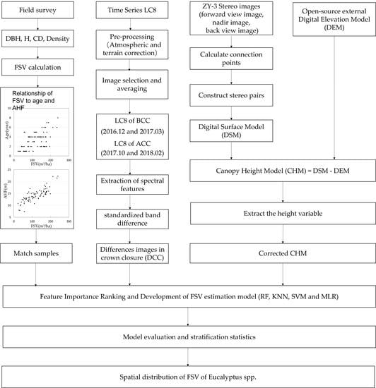
To improve the accuracy of FSV in planted eucalyptus forests, four Landsat 8 OLI and one pair of Ziyuan-3 (ZY-3) stereo images of planted eucalyptus forest were acquired before and after the crown closed, and the composite LC8 images were proposed to extract several new variables for reflecting the growth characteristics of the crown. Then, the CHM was obtained by subtracting the open-source DEM from the DSM extracted from the ZY-3 stereo images by the correction approach. Subsequently, four models (support vector machine (SVM), random forest (RF), k-nearest neighbors (KNN), and multiple linear regression (MLR)) were employed to estimate the FSV of the eucalyptus forest. The sensitivity and capability of stand age, CHM, and vegetation indices related to the growth characteristics of the crown were analyzed, and an optimal variable set related to crown characteristics was obtained to delay the saturation levels and to improve the accuracy of mapping FSV in the planted eucalyptus forest.

2. Materials and Methods

2.1. Study Area

The Gaofeng Forest Farm (Lat. 22°57′N, Lon. 108°19′E) is in the north of Nanning city, Guangxi Province, China (Figure 1). The landforms of the study area are mainly characterized by mountainous regions, with elevations up to 457 m in the northeast. The area has a subtropical monsoon climate, with an average annual temperature of 21 °C and an average annual rainfall of approximately 1200–1600 mm. The forest coverage rate in this region is greater than 80%, and the forest stock volume reached 6.63 million m3/ha in 2020 (https://www.gfslgy.com/, accessed on 8 May 2021). More than 90% of the study area is covered by planted forests, and the main tree species is eucalyptus.

2.2. Ground Data

Based on the stand age and spatial distribution in the study area, 87 samples (Figure 1) were randomly categorized into four forest ages (young forest (1-year-old), middle-age forest (2-year-old and 3-year-old), near-mature (4-year-old and 5-year-old) forest, and mature (older than 5 years) forest) in the planted eucalyptus forest. The corner and center positions of the ground samples were measured using global positioning system (GPS) device. In January 2018, these plots with a size of 20 m × 20 m were established, and the forest parameters (such as DBH, AFH, CD, density) were measured for each tree whose DBH was greater than 5 cm.
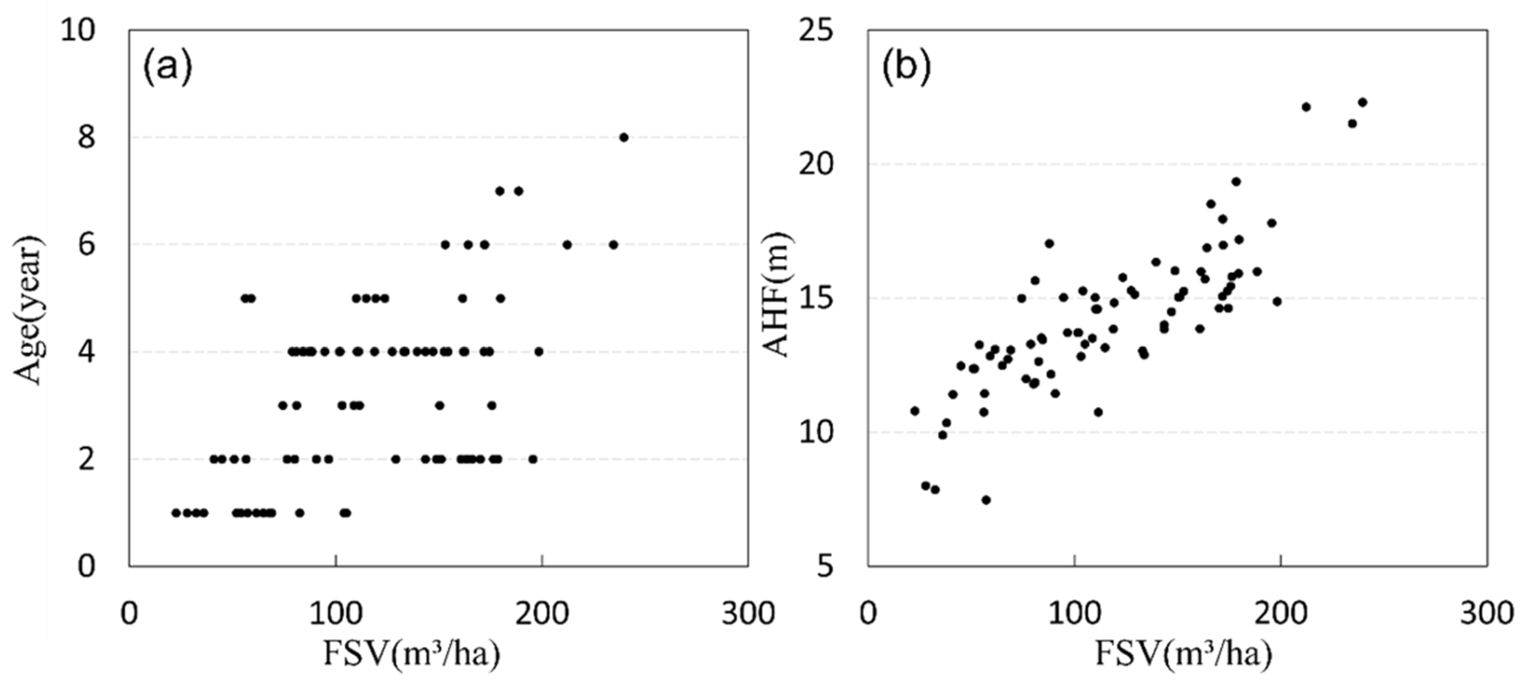
The volume of each tree was calculated using the binary volume table of the Gaofeng Forest Farm, and the FSV of each plot was obtained as the sum of the volume of all trees in the plots. The wood volume equation for Eucalyptus is derived from the technical regulations on construction of two-variable tree volume table of the People’s Republic of China (http://www.forestry.gov.cn, accessed on 8 May 2021). AHF was also obtained from the average height of all trees, and the stand age was obtained from the database of forest management investigation. The FSV of the ground-measured samples ranged from 22.6 to 239.5 m3/ha, with an average value of 118.1 m3/ha. The AHF ranged from 7.4 to 22.3 m, with an average value of 14.29 m. The relationships between FSV, age, and AHF are shown in Figure 2.

2.3. Processing the Remote Sensing Images

2.3.1. Extracting Variables from Landsat 8 OLI Data

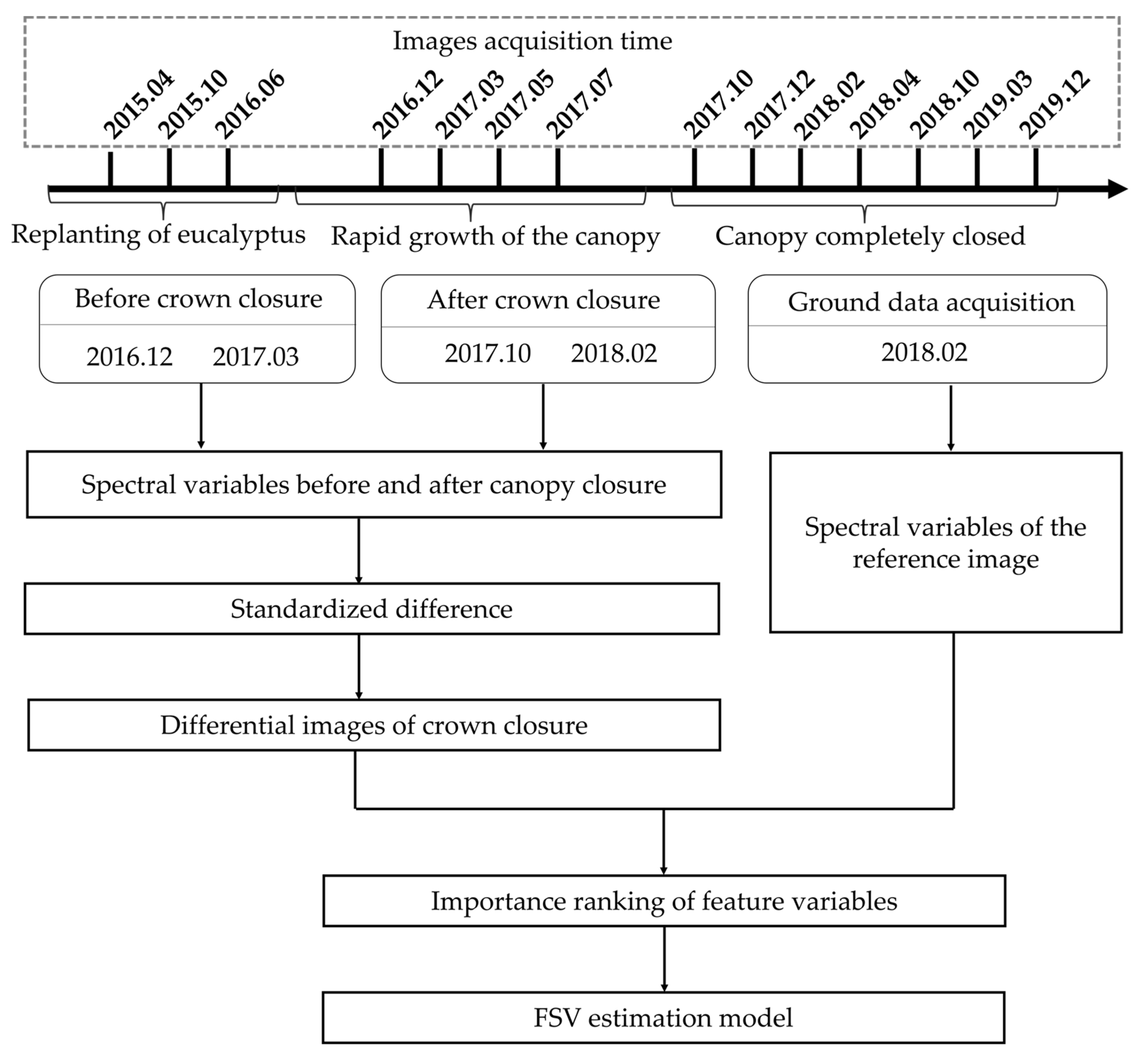
To retrieve the FSV of the eucalyptus forest, fourteen Landsat 8 OLI (LC8) remote sensing images with less than 5% cloud cover were downloaded from the US Geological Survey Earth Explorer website (http://earthexplorer.usgs.gov/, accessed on 10 June 2021). The acquisition dates of these images are shown in Figure 3 (ranged from 2015 to 2019). Based on the date of measurement of ground samples and crown characteristics, two images were acquired before the crown close (28 December 2016, and 2 March 2017), and two images were acquired after the crown close (28 October 2017, and 1 February 2018) were selected to form several new composite images in the next processing. Simultaneously, one of the images (acquired on 1 February 2018) was selected as the reference image to match the date of ground measurement. Atmospheric correction and relative radiometric calibration were performed using the regression equation to reduce errors due to differences in the acquired data. In each image, six multispectral bands with a spatial resolution of 30 m (three bands of visible light, one band of near-infrared, and two bands of shortwave infrared) were selected to extract the variables in the next process. Subsequently, an open-source DEM with a spatial resolution of 12.5 m was downloaded from NASA-EARTHDATA (https://search.asf.alaska.edu/, accessed on 11 June 2021).
To reduce the error of images, three composite images were proposed using algebraic operations of bands. Firstly, the average images before the crown close (BCC) were obtained from the images acquired on 28 December 2016, and 2 March 2017, and then the average images after the crown close (ACC) were obtained from the images acquired on 28 October 2017, and 1 February 2018. Furthermore, six bands (Band2_Blue, Band3_Green Band4_Red, Band5_NIR, Band6_SWIR1 and Band7_SWIR2) and six common vegetation indices, such as normalized difference vegetation index (NDVI), red–green vegetation index (RGVI), enhanced vegetation index (EVI), difference vegetation index (DVI), ratio vegetation index (RVI), and atmospherically resistant vegetation index (ARVI), were extracted from the two average images. Additionally, to improve the sensitivity between the vegetation indices and FSV, difference images were formed by subtracting images acquired before the crown close from the image acquired after the crown close (Figure 3). Therefore, variables derived from difference images are used to explore the sensitivity of FSV related to the growth characteristics of the crown. The standardized band difference was constructed as follows:
B D C C = ( B B C C B A C C ) ( B B C C + B A C C )
where BBCC is the band from the average images before the crown close, BACC is the band from the average images after the crown close, and BDCC is the band from the difference images before and after the crown close. After algebraic operations, variables (bands and vegetation indices) were extracted from the four LC8 images (three composite images and one reference image). Then, the importance of the alternative variables ranked by RF was employed to select the optimal variable set.

2.3.2. Extracting the CHM from ZY-3 Stereo Images

ZY-3 satellite data have been widely used to invert the DSM on a large scale [43,44,45]. Three images (forward image, orthorectified image and backward image) obtained from three high-resolution panchromatic cameras were used to provide the in-orbit stereo image pair. For this study, one pair of stereo images with a spatial resolution of 2.1 m was acquired in March 2018 (downloaded from Geospatial Data Cloud http://www.gscloud.cn/, accessed on 11 June 2021). Additionally, an open-source DEM with a spatial resolution of 12.5 m, downloaded from NASA-EARTHDATA (https://search.asf.alaska.edu/, accessed on 11 June 2021), was also used to extract the CHM. To accurately retrieve the DSM from ZY-3 stereo images, the steps of calculating connection points and regional network adjustment were initially employed to reconstruct the model of the point clouds, and the DSM was successfully derived from the model of point clouds after matching and interpolation. To match the resolution of the DSM, the DEM images were oversampled to a resolution of 2.1 m. Finally, the CHM was directly obtained by subtracting the open-source DEM from the extracted DSM. The above operation is performed in ENVI5.3 software.
In addition, height metrics were extracted as variables for correction CHM, including maximum height, minimum height, mean height, median height, and height profile quantiles (5 percent height (5 ph), 10 percent height (10 ph)…95 percent height (95 ph)). Additionally, then, to match the LC8 images, the spatial resolution of height variables were resampled to 30 m × 30 m. The corrected CHM (CCHM) was estimated using four algorithms (SVM, RF, KNN, and MLR) with the following variable sets, including the CHM data, spectral variables and stand age.

2.3.3. Variable Set

In this study, the bands and vegetation indices were derived from single (acquired on 1 February 2018) and composite images, respectively. Additionally, the stand age derived from a database of forest management investigation and CCHM derived from ZY-3 stereo images were employed to estimate the FSV. To explore the capability of mapping FSV, four types of alternative variables were divided into two groups: single and composite LC8 images, and four variable sets of each group were obtained from alternative variables selected by random forest (Table 1). The first set (variable set 1) included bands and vegetation indices extracted from single and composite LC8 images, the second variable set (variable set 2) included variable set 1 and the stand age, the third variable set (variable set 3) included the variable set 1 and CCHM, and the last set (variable set 4) included the variable set 1, stand age, and CCHM.

2.4. Model and Assessment

Recently, machine learning approaches have been widely used in the mapping of FSV. In this study, three machine learning models—SVM, RF, and KNN—and the multiple linear regression model (MLR) were employed to estimate the FSV in planted eucalyptus forest. Furthermore, leave-one-out cross-validation (LOOCV) was employed to assess the accuracy of the estimated FSV, and the root mean square error (RMSE), relative RMSE (RRMSE), and coefficient of determination (R2) were used as indicators to evaluate the accuracy of the model. The formulae are as follows:
R 2 = 1 ( y i y ^ i ) 2 ( y i y ^ i ) 2
R M S E = 1 N i = 1 N ( y i y ^ i ) 2
R R M S E = R M S E y ¯ × 100 %
where N is the number of samples, y is the observed value of FSV, y ^ is the estimated value of FSV, and y ¯ is the average of the observed values of FSV for all samples.

3. Results

3.1. The Growth Characteristics of Crown in Planted Eucalyptus Forest

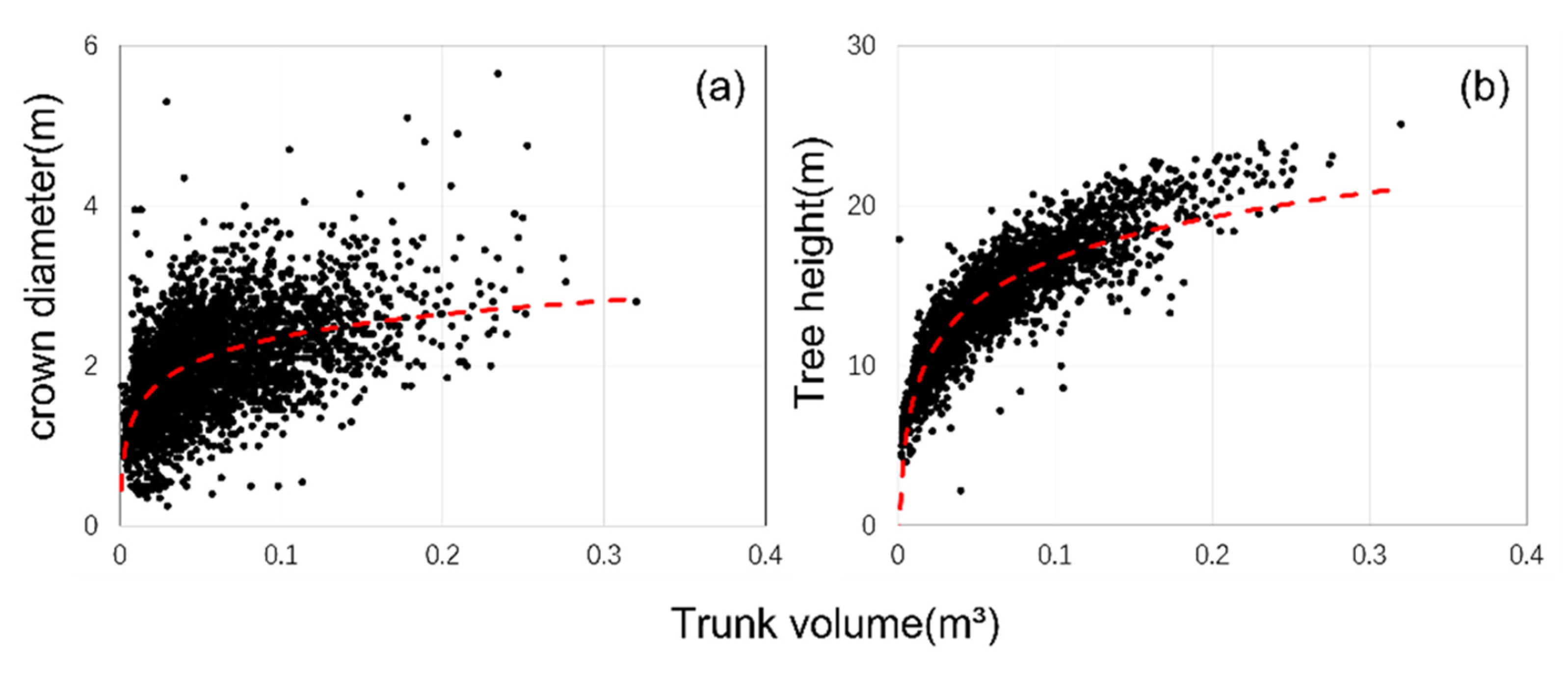
In planted eucalyptus forest, the FSV can be successfully detected by optical remote sensing images. The main reason is that the crown width changes with FSV during the growth before the crown close. After the crown closed, the saturation phenomenon occurred for optical remote sensing images. In our study, the parameters of near to 3000 trees were measured in all samples and scatterplots between the crown width, height and volume were shown in Figure 4.
It was found that the volume of tree varied significantly with increasing crown width at the very young stage (nearly to 2 years) and the sensitivity between the FSV and spectral variables was obviously high (Figure 4a). However, the sensitivity gradually decreased with the increasing volume of tree, because of unchanged crown width after a certain age. Finally, the saturation phenomenon occurred for mapping FSV using spectral variables in the planted eucalyptus forest. At this moment, the increased volume was mainly reflected by tree height (Figure 4b). Therefore, the growth characteristics of the crown and height of trees should be considered to improve the accuracy of mapping FSV at different growth stages.
Furthermore, four regions of planted eucalyptus forest were also selected to analyze the relationship between growth characteristics of the crown and NDVI extracted from fourteen images in five years (Figure 5). It is inferred that these regions were cut down and planted again between April 2015 and June 2016, and the results were also proved by time series NDVI. Meanwhile, the values of NDVI increased for about 2 years (from October 2015 to July 2017). After that, the NDVI values did not increase with the growth of eucalyptus forest, and the spectral characteristics of the crown did not reflect the increase in FSV. Therefore, variables extracted from single optical images have great potential for young eucalyptus forest (less than 2 years). However, for the middle-age, near-mature, and mature eucalyptus forest, the saturation phenomenon related to the crown will induce unacceptable errors for mapping FSV.

3.2. The Sensitivity of Variables Related to Width

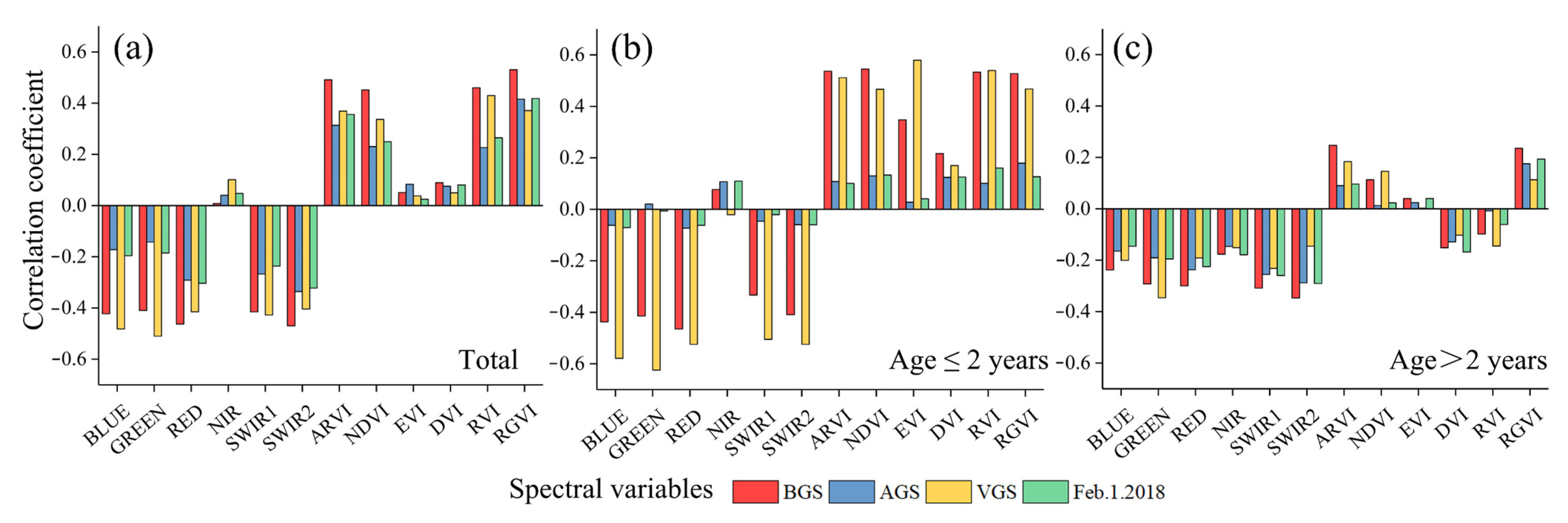
It has been reported that the width and depth of the eucalyptus crown are not sensitive to the FSV once the stand age reaches a certain age. To further explore the sensitivity between the FSV and spectral variables, three composite images, including two average images (BCC and ACC) and one difference image (DCC), were proposed to extract the variable set. Meanwhile, one single image (acquired on 1 February 2018) was also employed. Additionally, then, six bands and six indices were extracted from single and composite images, respectively. Additionally, all ground samples were divided into two groups: the first group was the samples with ages less than 2 years and the rest were the second group. The Pearson correlation coefficients between spectral variables and FSV were used to analyze the sensitivity of spectral variables related to growth characteristics of the crown in eucalyptus forest (Figure 6).
For all samples (Figure 6a), the Pearson correlation coefficient of each spectral variable extracted from single images (ranging from −0.4 to 0.4) was lower than that extracted from the composite images. Additionally, the spectral variable set extracted from DCC had the highest values of correlation. It was also observed that the sensitivities between FSV and spectral variables extracted from average (BCC) and composite (DCC) images were significantly higher than that extracted from single and average (ACC) images. It was proved that the sensitivity of spectral variables was severely affected by the growth characteristics of the crown. For the young eucalyptus forest (Figure 6b), variables extracted from average (BCC) and composite (DCC) images can capture the difference of FSV before the crown is closed. After the crown is closed, the results are contrary, such as the variables extracted from single and average (ACC) images.
Furthermore, for the first group, the spectral variables extracted from BCC and DCC had higher absolute value of correlation with FSV than those extracted from ACC and single images (Figure 6b). Additionally, the results show a small difference in the Pearson correlation coefficient from various images for the second group (Figure 6c). It was confirmed that the saturation of the spectral variable occurred at the stage of the closed crown. After that, the crown of eucalyptus did not grow with FSV because of the automatic pruning of eucalyptus. Therefore, the growth characteristics of the crown are helpful to select appropriate images and features (BCC and DCC images), and composite images have great potential to improve the accuracy of mapping FSV, especially for young eucalyptus forests.
Additionally, to map the FSV of the eucalyptus forest, an importance assessment method based on random forest was employed to select the optimal variable set. The ranking of the importance of the spectral variables is shown in Figure 7. For the reference LC8 images, RGVI was the most important and SWIR2 was the least important (Figure 7a). For the composite LC8 images, RGVI (derived from BCC) was the most important variable and DVI (derived from BCC) was the least important variable among all alternative variables (Figure 7b).

3.3. The Results of Extracted CHM

Using the ZY-3 stereo images, the CHM was directly extracted from the DSM by subtracting the open-sourced DEM, and a height variable with a size of 30 m × 30 m was extracted from the extracted CHM. Because of the errors from DEM, the gaps between the extracted CHM and ground-measured average height were so large that the height variable was difficult to apply directly in mapping FSV (Figure 8(a1)). To correct the CHM, vegetation indices, stand age, and height variable were employed to update the CHM using four models (MLR, KNN, SVM, and RF). The results of the CCHM are listed in Table 2.
For the single LC8 images, the RMSE of the estimated CCHM ranged from 2.06 to 2.52 m, respectively. Additionally, the optimal results were obtained using the KNN model. For the composite LC8 images, the RMSE of estimated CCHM ranged from 1.82 to 2.16 m, respectively. The accuracy of the estimated CCHM using variables extracted from composite LC8 images was slightly higher than that extracted from single LC8 images, and the optimal results were obtained from the RF model (R2 = 0.56, RMSE = 1.82 m). To further analyze the results of CCHM, scatterplots between CCHM and AHF were illustrated in Figure 8(b1,c1). After correcting the CHM, the Pearson correlation coefficient (r) between the CCHM and AHF increased significantly (from 0.48 to 0.75) using variable set extracted from composite LC8 images. Meanwhile, the values of the Pearson correlation coefficient between CCHM and FSV were up to 0.7 for single LC8 images and 0.76 for composite LC8 images, respectively.
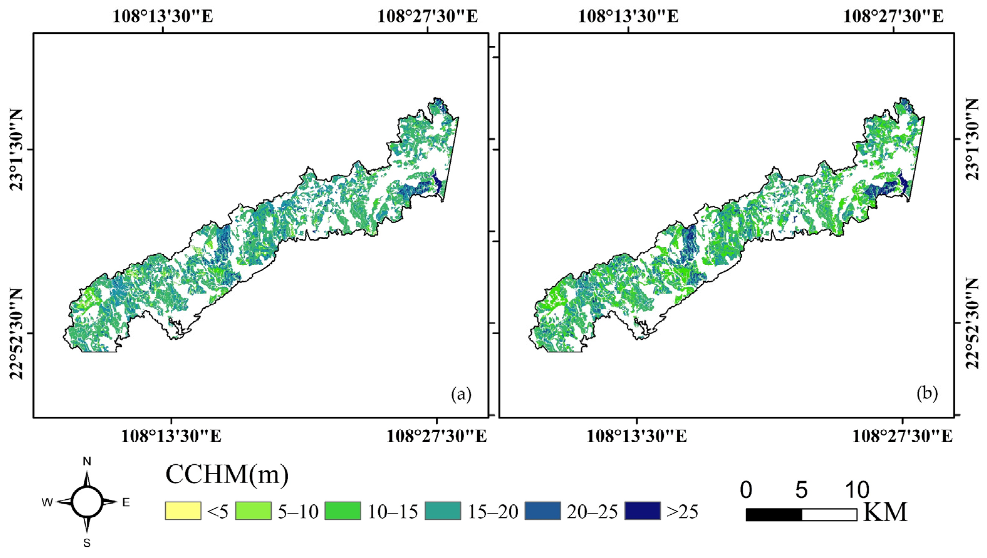
To map the results of CHM, vegetation indices extracted from the single and composite LC8 images were employed to retrieve CCHM using optimal models and other variable sets (stand age 5ph), respectively. Additionally, Figure 9 illustrates the results of mapped CCHM ranging from 10 to 20 m. Additionally, the CCHM extracted from various images was used for their respective FSV estimations in the next process.

3.4. The Results of Mapped FSV

To accurately map the FSV of planted eucalyptus forest, four models (SVM, RF, KNN, and MLR) were employed to construct the relationship between the FSV and various optimal variable sets. In this study, four types of optimal variable sets were extracted from single and composite LC8 images, and the results of the estimated FSV are listed in Table 3. In each variable set, the best results were obtained using different models, and the differences between the models were within 5%. The results indicate that the models were not the main factors affecting the accuracy of the mapping FSV.
Table 3 also illustrates that the variable set extracted from various images, stand age, and CCHM played different roles in improving the accuracy of mapping FSV. For each variable set, the RRMSEs of estimated FSV with the vegetation indices extracted from composite LC8 images were significantly smaller than those extracted from single LC8 images, and the differences gradually narrowed as the stand age and CCHM were added to the variable set. It was confirmed that the variables extracted from the composite LC8 images were more sensitive than those extracted from the single LC8 images. Furthermore, after adding CCHM to variable set 1, the average RRMSEs of the four employed models decreased from 41.01% to 31.08% for single LC8 images and from 32.64% to 29.13% for composite LC8 images, respectively. The highest accuracy of the estimated FSV was obtained in the case of variable set 4. It was concluded that the parameters of stand age and CCHM have great potential in improving the accuracy of estimated FSV in planted eucalyptus forests.
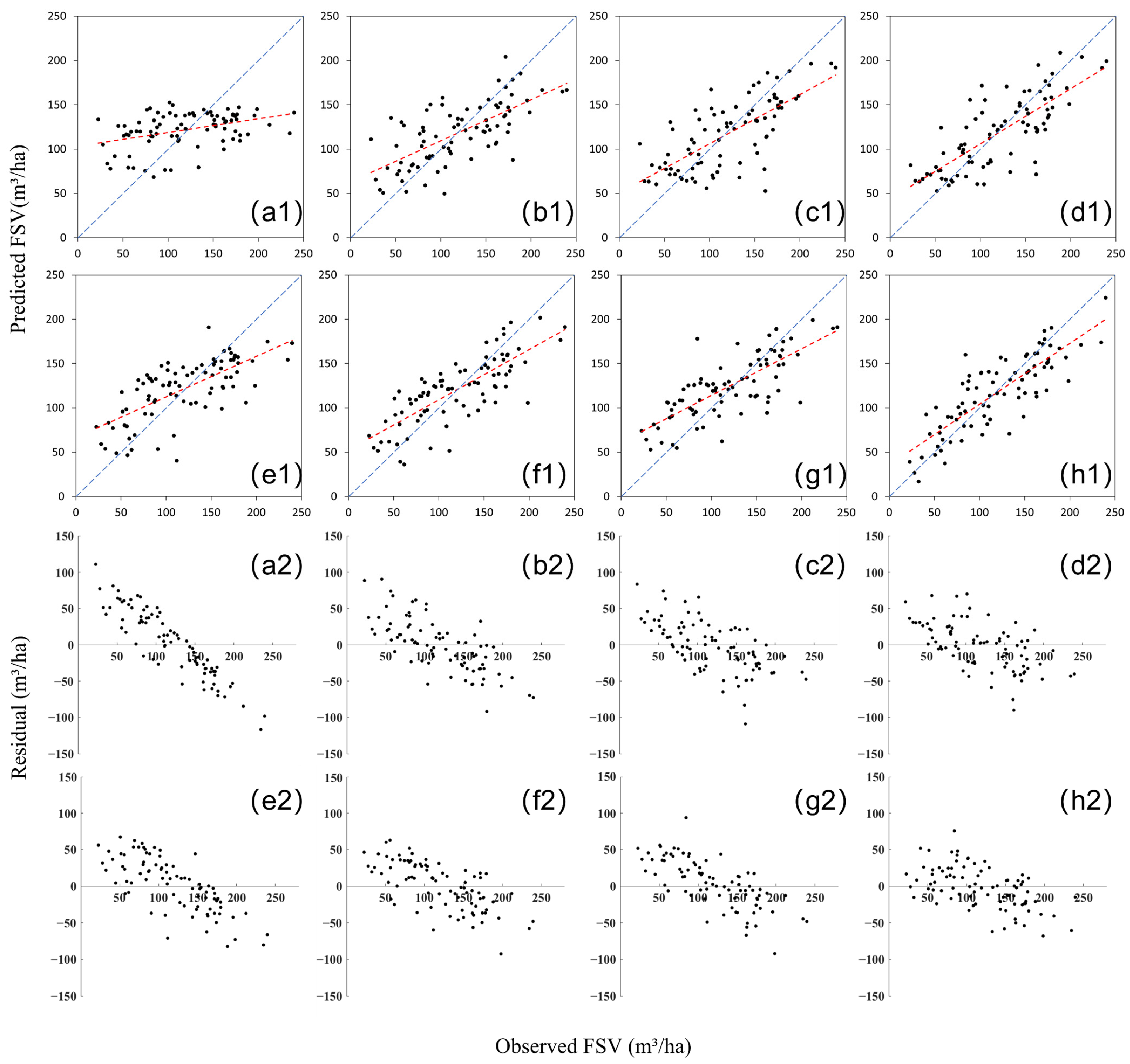
To further analyze the contribution of various variables, Figure 10(a1–h1) illustrates the scatterplots between the ground measured and predicted FSV using the models with the highest accuracy of results in each variable set (Table 3). The residuals of each selected model are also plotted in Figure 10(a2–h2). For young samples (stand age: less than 2 years), overestimated results frequently occurred using the variable set extracted from single LC8 images (Figure 10(a1,a2)). The results were significantly improved using the variable set extracted from composite LC8 images (Figure 10(e1,e2). Therefore, it was inferred that composite LC8 images could improve the accuracy of FSV for young eucalyptus forests.
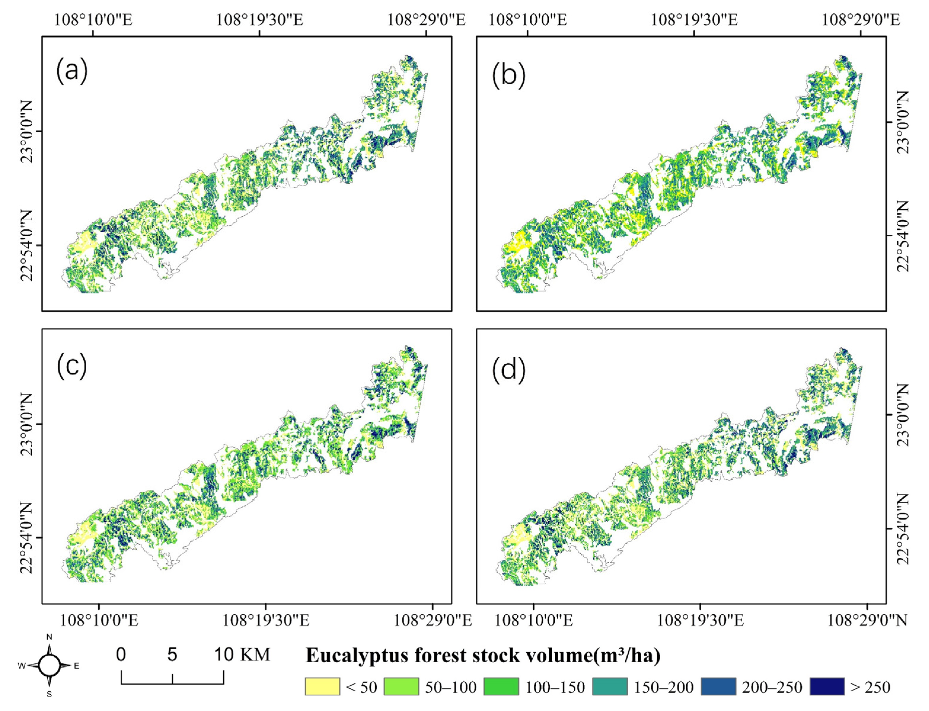
Moreover, without the stand age and CCHM, the saturation levels occurred at a low FSV (approximately 100–150 m3/ha), and the accuracy of the results was severely influenced by FSV underestimated samples (Figure 10(e1,e2)). After adding the CCHM and stand age, the accuracy of the estimated FSV improved significantly as the number of underestimated samples decreased. The residuals of variable set 2 (Figure 10(f2)) and variable set 3 (Figure 10(g2)) were close to zero after adding the CCHM and stand age, and the highest accuracy of estimated FSV (R2 = 0.68, RMSE = 24.04%) was obtained in the case of variable set 4 (Figure 10(h1)). Therefore, the CCHM and stand age are useful to improve the accuracy of mapping FSV by delaying saturation levels. Finally, the FSV of the study area was mapped using four models and variable set 4 extracted from the composite LC8 images (Figure 11). There was no obvious difference between each employed model in the spatial distribution of the FSV. Furthermore, it was also observed that the FSVs ranged from 50 to 200 m3/ha in most of the eucalyptus forest.

4. Discussion

4.1. Challenges in Mapping FSV of Eucalyptus Using Optical Images

In previous studies, it has been proven that optical and microwave images can be successfully applied to map FSV or AGB, owing to the high correlation between the spectral features [11,16,29]. However, it was difficult to obtain a high correlation between the spectral variables extracted from the single LC8 images and the FSV in our study, and the accuracy of the estimated FSV (R2 less than 0.2) was rather low using single LC8 images in the planted eucalyptus forest. Additionally, it was observed that the characteristics of SAR images also made it difficult to estimate the FSV of eucalyptus [23]. Due to the growth characteristics of the crown in planted eucalyptus forests, it has been observed that mapping the FSV of eucalyptus forests is more challenging than other tree species (such as coniferous forests). It has been reported that the crown of young eucalyptus changes with FSV before the crown close, and the sensitivity between spectral variables and FSV decreases with age once the stand reaches a certain age (occurred saturation) [24].
Naturally, the saturation levels can be delayed by combining auxiliary data, such as stand age and forest height. Similarly, the importance of age in estimating FSV in eucalyptus plantations has been highlighted in a previous study [22,45]. To improve the accuracy of FSV in the planted eucalyptus forest, composite Landsat 8 images and ZY-3 stereo images were proposed to obtain vegetation indices and forest height, respectively. Table 3 and Figure 9 illustrate that the accuracy of mapped FSV of eucalyptus forest was successfully improved using CCHM and spectral variables extracted from composite images, and the numbers of overestimated and underestimated samples obviously decreased. Therefore, it was inferred that spectral variables from composite images have the capability to estimate the FSV of eucalyptus forests based on the growth characteristics of the crown.
In addition, three non-parametric models (RF, KNN and SVM) and one parametric model (MLR) were widely employed for mapping FSV. MLR was found to have weaker estimation power than the nonparametric models (e.g., variable set 1 and variable set 2) when the correlation between remote sensing variables and FSV was not high. This result can be attributed to the fact that parametric models can only represent linear relationships between variables and FSV [18,19,46,47], while the relationships between remote sensing variables and FSV may be nonlinear due to the complex forest environment. When remote sensing variables with higher correlation with FSV (e.g., CCHM) were entered into the model, approximate results were obtained when FSV was estimated using the four models (variable set 3). In conclusion, compared to parametric models, nonparametric models can identify potential relationships between remote sensing variables and FSV and have higher flexibility in that it does not need to consider covariance between variables with specific sample distributions (e.g., normal distribution) and has greater potential for quantification and mapping species of forest parameters.

4.2. The Effect of Crown, Forest Height and Stand Age on Mapping FSV

In the previous study, the spectral variables extracted from the optical images have been proved to be insensitive to changes in FSV in planted eucalyptus forests [23]. In this study, it was also observed that the width and depth of the eucalyptus crown were not sensitive to the FSV once the stand reached a certain age (Figure 6). Furthermore, to use phenological information on vegetation growth, multi-temporal remote sensing images have been regarded as a significant advantage in obtaining forest parameters, especially for vegetation with significant seasonal changes [25,27,28]. In a previous study, multi-temporal optical images were successfully used to estimate the forest structure parameters [18,36,43]. In our study, three composite images were proposed from acquired fourteen LC8 images using algebraic operations of bands. The results indicate that the Pearson correlation coefficient of each spectral variable extracted from single LC8 images (ranging from −0.4 to 0.4) was lower than that extracted from composite images (BCC and DCC). Additionally, the variables extracted from composite images (BCC and DCC) were more sensitive than those extracted from single and ACC images for young eucalyptus forests. The main reason is that the increased FSV can be reflected by changes in the forest crown for young eucalyptus forests before the crown close.
Without penetrating the dense crown, optical remote sensing data will inevitably exhibit spectral saturation for estimating FSV or AGB [5,17,48]. Recently, CHM has been closely related to FSV without the data saturation problem; it is regarded as an effective approach to overcome the problem of spectral saturation [13,43,49,50,51]. At present, stereo images have great potential for extracting forest height with an accurate DEM or digital terrain module (DTM). Several studies have successfully extracted forest height using DSM during the peak and deciduous seasons; however, this approach is only applicable to deciduous tree species such as larch [44]. In this study, the CHM of eucalyptus stands was directly extracted by open-sourced DEM, and the RMSEs ranged from 2.06 to 1.82 m after correction. After adding the CCHM for estimating FSV, the average errors decreased from −46.7 to −27.89 m3/ha for single LC8 images and from −30.60 to −20.82 m3/ha for multitemporal LC8 images (Table 3). Although the accuracy of CCHM is certainly lower than that of LiDAR, it was confirmed that CCHM, which is regarded as an indirect variable, can significantly improve the estimated FSV in eucalyptus forests.
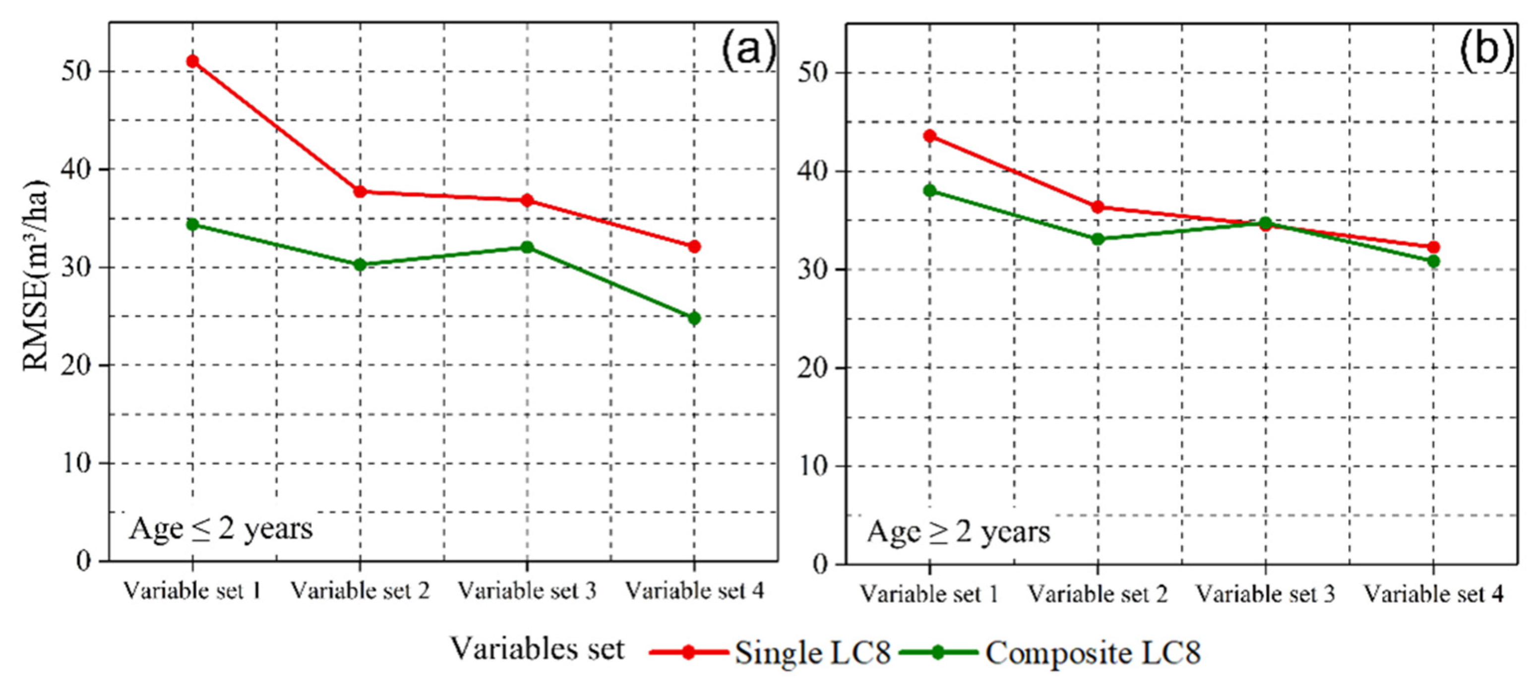
To further analyze the contributions of the crown width, forest height and stand age to map FSV, all samples were divided into two groups based on stand age: the first group is stand age younger than two years old and the rest is the second group (stand age > 2 years). Using the proposed composite images, the overestimated FSV was significantly decreased because of the contribution of the crown width, and Figure 12 illustrates that the contributions of the crown in young samples (RMSE reduced by 15%) is obviously larger than that in near-mature or mature samples (RMSE reduced by 5%). Moreover, the contributions of the crown width gradually faded into insignificance for near-mature or mature eucalyptus forest. These results also indicated that composite LC8 images were more capable of improving the accuracy of FSV in young eucalyptus forests. The main reason is the growth characteristics of the crown; the crown of young eucalyptus grows with an increase in FSV. In contrast, it is rather difficult to obtain a reliable FSV using single LC8 images after crown closure because of saturation problems.
On the contrary, the forest height made a great contribution for mapping FSV, whether young or mature eucalyptus forest. For young forest, the contributions of forest height (CHM) and stand age using single LC8 images are larger than those using composite images (Figure 12a). Therefore, it was confirmed that the CCHM improved the accuracy of the estimated FSV for high FSV forests (near mature and mature eucalyptus). Additionally, upon using the stand age and CCHM, the accuracy of the estimated FSV was also improved for the low and high FSV forests.

5. Conclusions

To overcome the limitations of small canopies in eucalyptus forests, time series Landsat 8 OLI images were acquired before and after the crown close, and one pair of stereo images was employed to derive the CHM. After forming the composite images, various vegetation indices and bands were extracted to analyze the response of the FSV to the crown close and other forest parameters. The results show that the FSV of eucalyptus forest could be successfully obtained by combining multi-temporal LC8 with stand age and CCHM. The number of samples with overestimated and underestimated FSV was reduced. In addition, the results also show that the corrected CHM, which is regarded as an indirect variable, can significantly improve the accuracy of estimated FSV in eucalyptus forests, especially for near-mature and mature forests. It was also confirmed that variables extracted from seasonal LC8 images were more sensitive to the FSV in young eucalyptus forests. In contrast, it is rather difficult to obtain a reliable FSV using single LC8 images after crown closure. In the future, seasonal variables associated with the crown close will be extracted from other optical remote sensing images, and the precise response will be analyzed to describe the relationship between the various variables and FSV for determining the specific saturation levels in planted eucalyptus forests.

Author Contributions

Conceptualization, Z.L., J.L. and H.L.; methodology, Z.L., X.X. and J.L.; software, Z.L.; validation, Z.L., J.L. and H.L.; formal analysis, Z.L., Z.Y., T.Z. and X.X.; investigation, Z.L., J.L., H.L. and Z.Y.; resources, Z.L., X.X., J.L. and Z.Y.; data processing, Z.L. and X.X.; original draft, Z.L.; review and revision, Z.L., J.L. and H.L.; final editing: J.L.; visualization, Z.L., J.L. and T.Z.; supervision, H.L. and J.L.; project administration, Z.L. and J.L.; funding acquisition, Z.L., J.L., X.X. and H.L. All authors have read and agreed to the published version of the manuscript.

Funding

This research was funded by the Innovative and Construction special funds of Hunan Province “Intelligent measurement and monitoring technology of forest stock, biomass and carbon storage based on multi-source data of land, space and sky” (2020NK2051), National Key R&D Program of China project “Research of Key Technologies for Monitoring Forest Plantation Resources” (2017YFD0600900), postgraduate scientific research Innovative project of Hunan province “Study on Estimation of Eucalyptus Plantation Volume Based on Combining Stereo Data and Landsat 8 OLI Time Series” (CX20210854), and “Research on remote sensing estimation of plantation growing stem volume based on integrated learning algorithm” (CX20220703).

Data Availability Statement

The observed GSV data from the sample plots and spatial distribution data of forest resources presented in this study are available on request from the corresponding author. Those data are not publicly available due to privacy and confidentiality. The Landsat 8 OLI and ZY-3 stereo data were obtained from the US Geological Survey Earth Explorer website (http://earthexplorer.usgs.gov/, accessed on 11 June 2021).

Conflicts of Interest

The authors declare no conflict of interest.

References

  1. Brockerhoff, E.G.; Jactel, H.; Parrotta, J.A.; Ferraz, S.F. Role of eucalypt and other planted forests in biodiversity conservation and the provision of biodiversity-related ecosystem services—ScienceDirect. For. Ecol. Manag. 2013, 301, 43–50. [Google Scholar] [CrossRef]
  2. Dube, T.; Sibanda, M.; Shoko, C.; Mutanga, O. Stand-volume estimation from multi-source data for coppiced and high forest Eucalyptus spp. silvicultural systems in KwaZulu-Natal, South Africa. ISPRS J. Photogramm. 2017, 132, 162–169. [Google Scholar] [CrossRef]
  3. Li, X.; Ye, D.; Liang, H.; Zhu, H.; Lin, Q.; Zhu, Y.; Wen, Y. Effects of Successive Rotation Regimes on Carbon Stocks in Eucalyptus Plantations in Subtropical China Measured over a Full Rotation. PLoS ONE 2015, 10, e132858. [Google Scholar] [CrossRef] [PubMed] [Green Version]
  4. Cosmo, L.D.; Gasparini, P.; Tabacchi, G. A national-scale, stand-level model to predict total above-ground tree biomass from growing stock volume. For. Ecol. Manag. 2016, 361, 269–276. [Google Scholar] [CrossRef]
  5. Jiang, F.; Kutia, M.; Sarkissian, A.J.; Lin, H.; Long, J.; Sun, H.; Wang, G. Estimating the Growing Stem Volume of Coniferous Plantations Based on Random Forest Using an Optimized Variable Selection Method. Sensors 2020, 20, 7248. [Google Scholar] [CrossRef]
  6. Long, J.; Lin, H.; Wang, G.; Sun, H.; Yan, E. Mapping Growing Stem Volume of Chinese Fir Plantation Using a Saturation-based Multivariate Method and Quad-polarimetric SAR Images. Remote Sens. 2019, 11, 1872. [Google Scholar] [CrossRef] [Green Version]
  7. Ismail, R. Assessing the utility of ALOS PALSAR and SPOT 4 to predict timber volumes in even-aged Eucalyptus plantations located in Zululand, South Africa. J. S. Afr. For. Assoc. 2015, 77, 203–211. [Google Scholar] [CrossRef]
  8. Berger, A.; Gschwantner, T.; McRoberts, R.E.; Schadauer, K. Effects of Measurement Errors on Individual Tree Stem Volume Estimates for the Austrian National Forest Inventory. For. Sci. 2014, 60, 14–24. [Google Scholar] [CrossRef]
  9. Asner, G.P.; Alencar, A. Drought impacts on the amazon forest: The remote sensing perspective. New Phytol. 2010, 187, 569–578. [Google Scholar] [CrossRef]
  10. Dengsheng, L. The potential and challenge of remote sensing-based biomass estimation. Int. J. Remote Sens. 2006, 27, 1297–1328. [Google Scholar] [CrossRef]
  11. Roberts, J.W.; Van Aardt, J.A.N.; Ahmed, F.B. Image fusion for enhanced forest structural assessment. Int. J. Remote Sens. 2011, 32, 243–266. [Google Scholar] [CrossRef]
  12. Franco-Lopez, H.; Ek, A.R.; Bauer, M.E. Estimation and mapping of forest stand density, volume, and cover type using the k-nearest neighbors method. Remote Sens. Environ. 2001, 77, 251–274. [Google Scholar] [CrossRef]
  13. Lim, K.; Treitz, P.; Wulder, M.; St-Onge, B.; Flood, M. LiDAR remote sensing of forest structure. Prog. Phys. Geogr. 2003, 27, 88–106. [Google Scholar] [CrossRef] [Green Version]
  14. Balenović, I.; Milas, A.S.; Marjanović, H. A Comparison of Stand-Level Volume Estimates from Image-Based Canopy Height Models of Different Spatial Resolutions. Remote Sens. 2017, 9, 205. [Google Scholar] [CrossRef] [Green Version]
  15. Narine, L.L.; Popescu, S.C.; Malambo, L. Synergy of ICESat-2 and Landsat for Mapping Forest Aboveground Biomass with Deep Learning. Remote Sens. 2019, 11, 1503. [Google Scholar] [CrossRef]
  16. Wijaya, A.; Kusnadi, S.; Gloaguen, R.; Heilmeier, H. Improved strategy for estimating stem volume and forest biomass using moderate resolution remote sensing data and GIS. J. For. Res. 2010, 21, 1–12. [Google Scholar] [CrossRef]
  17. Fugen, J.; Feng, Z.; Kaisen, M.; Dongsheng, L.; Hua, S. Mapping the Forest Canopy Height in Northern China by Synergizing ICESat-2 with Sentinel-2 Using a Stacking Algorithm. Remote Sens. 2021, 13, 1535. [Google Scholar] [CrossRef]
  18. Li, X.; Liu, Z.; Lin, H.; Wang, G.; Zhang, M. Estimating the Growing Stem Volume of Chinese Pine and Larch Plantations based on Fused Optical Data Using an Improved Variable Screening Method and Stacking Algorithm. Remote Sens. 2020, 12, 871. [Google Scholar] [CrossRef] [Green Version]
  19. Wang, Y.; Zhang, X.; Guo, Z. Estimation of tree height and aboveground biomass of coniferous forests in North China using stereo ZY-3, multispectral Sentinel-2, and DEM data. Ecol. Indic. 2021, 126, 107645. [Google Scholar] [CrossRef]
  20. Foody, G.M.; Boyd, D.S.; Cutler, M.E.J. Predictive relations of tropical forest biomass from Landsat TM data and their transferability between regions. Remote Sens. Environ. 2003, 85, 463–474. [Google Scholar] [CrossRef]
  21. Gemmell, F.M. Effects of forest cover, terrain, and scale on timber volume estimation with Thematic Mapper data in a Rocky Mountain site. Remote Sens. Environ. 1995, 51, 291–305. [Google Scholar] [CrossRef]
  22. Zhao, P.; Lu, D.; Wang, G.; Liu, L.; Li, D.; Zhu, J.; Yu, S. Forest aboveground biomass estimation in Zhejiang Province using the integration of Landsat TM and ALOS PALSAR data. Int. J. Appl. Earth Obs. Geoinf. 2016, 53, 1–15. [Google Scholar] [CrossRef]
  23. Almeida, A.C.; Soares, J.V.; Landsberg, J.J.; Rezende, G.D. Growth and water balance of Eucalyptus grandis hybrid plantations in Brazil during a rotation for pulp production. For. Ecol. Manag. 2007, 251, 10–21. [Google Scholar] [CrossRef]
  24. Wei, C.; Huang, J.; Mansaray, L.R.; Li, Z.; Liu, W.; Han, J. Estimation and Mapping of Winter Oilseed Rape LAI from High Spatial Resolution Satellite Data Based on a Hybrid Method. Remote Sens. 2017, 9, 488. [Google Scholar] [CrossRef] [Green Version]
  25. Su, W.; Huang, J.; Liu, D.; Zhang, M. Retrieving Corn Canopy Leaf Area Index from Multitemporal Landsat Imagery and Terrestrial LiDAR Data. Remote Sens. 2019, 11, 572. [Google Scholar] [CrossRef] [Green Version]
  26. Zhou, H.; Wang, J.; Liang, S.; Xiao, Z. Extended Data-Based Mechanistic Method for Improving Leaf Area Index Time Series Estimation with Satellite Data. Remote Sens. 2017, 9, 533. [Google Scholar] [CrossRef] [Green Version]
  27. Gasparri, N.I.; Parmuchi, M.G.; Bono, J.; Karszenbaum, H.; Montenegro, C.L. Assessing multi-temporal Landsat 7 ETM+ images for estimating above-ground biomass in subtropical dry forests of Argentina. J. Arid Environ. 2010, 74, 1262–1270. [Google Scholar] [CrossRef]
  28. Mikhail, U.; Christian, T.; Mirco, M.; Markus, R.; Pedro, R.V.; Christiane, S. Improved Multi-Sensor Satellite-Based Aboveground Biomass Estimation by Selecting Temporally Stable Forest Inventory Plots Using NDVI Time Series. Forests 2016, 7, 169. [Google Scholar] [CrossRef] [Green Version]
  29. Reiche, J.; Hamunyela, E.; Verbesselt, J.; Hoekman, D.; Herold, M. Improving near-real time deforestation monitoring in tropical dry forests by combining dense Sentinel-1 time series with Landsat and ALOS-2 PALSAR-2. Remote Sens. Environ. 2018, 204, 147–161. [Google Scholar] [CrossRef]
  30. Ji, L.; Wylie, B.K.; Nossov, D.R.; Peterson, B.; Waldrop, M.P.; McFarland, J.W.; Rover, J.; Hollingsworth, T.N. Estimating aboveground biomass in interior Alaska with Landsat data and field measurements. Int. J. Appl. Earth Obs. 2012, 18, 451–461. [Google Scholar] [CrossRef]
  31. Ginzler, C.; Hobi, M.L. Countrywide Stereo-Image Matching for Updating Digital Surface Models in the Framework of the Swiss National Forest Inventory. Remote Sens. 2015, 7, 4343–4370. [Google Scholar] [CrossRef] [Green Version]
  32. Ghosh, S.M.; Behera, M.D. Aboveground biomass estimation using multi-sensor data synergy and machine learning algorithms in a dense tropical forest. Appl. Geogr. 2018, 96, 29–40. [Google Scholar] [CrossRef]
  33. Knapp, N.; Fischer, R.; Cazcarra-Bes, V.; Huth, A. Structure Metrics to Generalize Biomass Estimation from Lidar across Forest Types from Different Continents. Remote Sens. Environ. 2019, 237, 111597. [Google Scholar] [CrossRef]
  34. Mascaro, J.; Detto, M.; Asner, G.P.; Muller-Landau, H.C. Evaluating uncertainty in mapping forest carbon with airborne LiDAR. Remote Sens. Environ. 2011, 115, 3770–3774. [Google Scholar] [CrossRef]
  35. Shean, D.E.; Alexandrov, O.; Moratto, Z.M.; Smith, B.E.; Joughin, I.R.; Porter, C.; Morin, P. An automated, open-source pipeline for mass production of digital elevation models (DEMs) from very-high-resolution commercial stereo satellite imagery. ISPRS J. Photogramm. Remote Sens. 2016, 116, 101–117. [Google Scholar] [CrossRef] [Green Version]
  36. Lu, D.; Chen, Q.; Wang, G.; Liu, L.; Li, G.; Moran, E. A survey of remote sensing-based aboveground biomass estimation methods in forest ecosystems. Int. J. Digit. Earth 2016, 9, 63–105. [Google Scholar] [CrossRef]
  37. Antropov, O.; Rauste, Y.; Ahola, H.; Hame, T. Stand-Level Stem Volume of Boreal Forests from Spaceborne SAR Imagery at L-Band. IEEE J. Sel. Top. Appl. Earth Obs. Remote Sens. 2013, 6, 35–44. [Google Scholar] [CrossRef]
  38. Abdullahi, S.; Kugler, F.; Pretzsch, H. Prediction of stem volume in complex temperate forest stands using TanDEM-X SAR data. Remote Sens. Environ. 2016, 174, 197–211. [Google Scholar] [CrossRef]
  39. Chowdhury, T.; Thiel, C.; Schmullius, C.; Stelmaszczuk-Górska, M. Polarimetric Parameters for Growing Stock Volume Estimation Using ALOS PALSAR L-Band Data over Siberian Forests. Remote Sens. 2013, 5, 5725–5756. [Google Scholar] [CrossRef] [Green Version]
  40. Iizuka, K.; Tateishi, R. Simple Relationship Analysis between L-Band Backscattering Intensity and the Stand Characteristics of Sugi (Cryptomeria japonica) and Hinoki (Chamaecyparis obtusa) Trees. Adv. Remote Sens. 2014, 3, 219–234. [Google Scholar] [CrossRef]
  41. Lei, Y.; Siqueira, P. Estimation of Forest Height Using Spaceborne Repeat-Pass L-Band InSAR Correlation Magnitude over the US State of Maine. Remote Sens. 2014, 6, 10252–10285. [Google Scholar] [CrossRef] [Green Version]
  42. Ahmed, R.; Siqueira, P.; Hensley, S.; Chapman, B.; Bergen, K. A survey of temporal decorrelation from spaceborne L-Band repeat-pass InSAR. Remote Sens. Environ. 2011, 115, 2887–2896. [Google Scholar] [CrossRef]
  43. Zhang, T.; Lin, H.; Long, J.; Zhang, M.; Liu, Z. Analyzing the Saturation of Growing Stem Volume Based on ZY-3 Stereo and Multispectral Images in Planted Coniferous Forest. IEEE J. Sel. Top. Appl. Earth Obs. Remote Sens. 2021, 15, 50–61. [Google Scholar] [CrossRef]
  44. Li, G.; Xie, Z.; Jiang, X.; Lu, D.; Chen, E. Integration of ZiYuan-3 Multispectral and Stereo Data for Modeling Aboveground Biomass of Larch Plantations in North China. Remote Sens. 2019, 11, 2328. [Google Scholar] [CrossRef] [Green Version]
  45. Xie, Z.; Chen, Y.; Lu, D.; Li, G.; Chen, E. Classification of Land Cover, Forest, and Tree Species Classes with ZiYuan-3 Multispectral and Stereo Data. Remote Sens. 2019, 11, 164. [Google Scholar] [CrossRef] [Green Version]
  46. Zhang, C.; Denka, S.; Cooper, H.; Mishra, D.R. Quantification of sawgrass marsh aboveground biomass in the coastal Everglades using object-based ensemble analysis and Landsat data. Remote Sens. Environ. 2017, 204, 366–379. [Google Scholar] [CrossRef]
  47. Powell, S.L.; Cohen, W.B.; Healey, S.P.; Kennedy, R.E.; Moisen, G.G.; Pierce, K.B.; Ohmann, J.L. Quantification of live aboveground forest biomass dynamics with Landsat time-series and field inventory data: A comparison of empirical modeling approaches. Remote Sens. Environ. 2010, 114, 1053–1068. [Google Scholar] [CrossRef]
  48. Reis, A.D.; Franklin, S.E.; Mello, J.D.; Junior, F.A. Volume estimation in a Eucalyptus plantation using multi-source remote sensing and digital terrain data: A case study in Minas Gerais State, Brazil. Int. J. Remote Sens. 2019, 40, 2683–2702. [Google Scholar] [CrossRef]
  49. Zhu, X.; Liu, D. Improving Forest aboveground biomass estimation using seasonal Landsat NDVI time-series. ISPRS J. Photogramm. Remote Sens. 2015, 102, 222–231. [Google Scholar] [CrossRef]
  50. Immitzer, M.; Stepper, C.; Böck, S.; Straub, C.; Atzberger, C. Use of WorldView-2 stereo imagery and National Forest Inventory data for wall-to-wall mapping of growing stock. For. Ecol. Manag. 2016, 359, 232–246. [Google Scholar] [CrossRef]
  51. Vastaranta, M.; Yu, X.; Luoma, V.; Karjalainen, M.; Saarinen, N.; Wulder, M.A.; White, J.C.; Persson, H.J.; Hollaus, M.; Yrttimaa, T.; et al. Aboveground forest biomass derived using multiple dates of WorldView-2 stereo-imagery: Quantifying the improvement in estimation accuracy. Sci. Total Environ. 2019, 39, 8766–8783. [Google Scholar] [CrossRef]
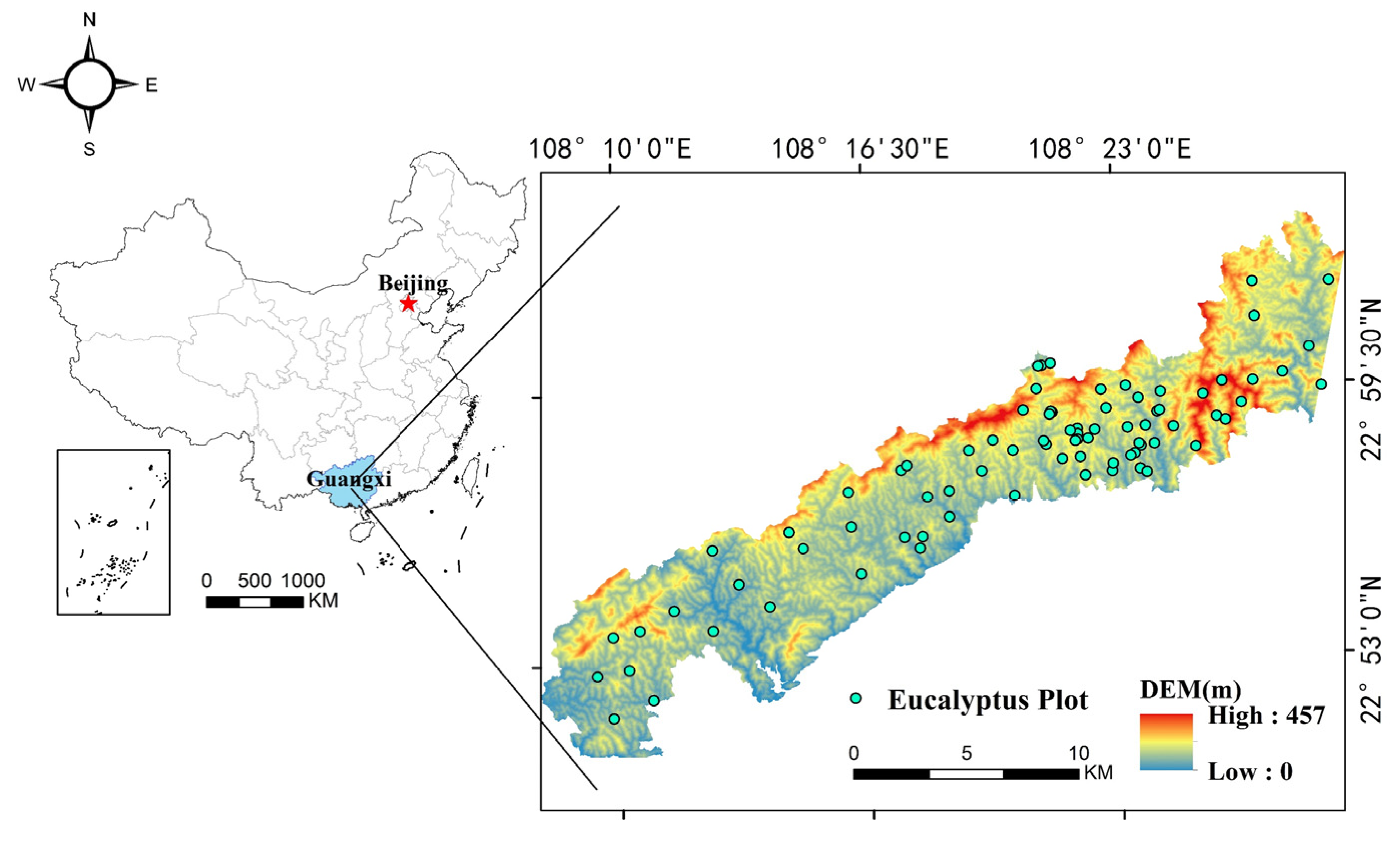
Figure 1. The location of the study area, and the distribution of the ground samples in planted eucalyptus forest.
Remotesensing 14 05082 g001
Figure 2. The relationship between AHF, age and FSV: (a) is the scatterplot of FSV and age; (b) is the scatterplot of FSV and AHF.
Remotesensing 14 05082 g002
Figure 3. The flowchart of composite LC8 images.
Remotesensing 14 05082 g003
Figure 4. The scatterplots between volume and measured parameters of single tree: the red dash line is the trend line of the scatter, (a) is the scatterplot between volume and crown width and (b) is the scatterplot between volume and tree height.
Remotesensing 14 05082 g004
Figure 5. The images of four regions with different stages and time series average NDVI of selected regions from April 2015 to December 2019, the red dashed box is used to highlight the change in NDVI of eucalyptus over time, which gradually increases inside the red dashed box and stops changing outside the red dashed box.
Remotesensing 14 05082 g005
Figure 6. The histograms of Pearson Correlation coefficient between spectral variables and FSV: (a) illustrates all samples; (b) illustrates the samples with stand age less than 2 years; (c) illustrates the samples with stand age larger than 2 years.
Remotesensing 14 05082 g006
Figure 7. The importance of spectral variables: (a) is variables extracted from single LC8 images; (b) is variables extracted from composite LC8 images.
Remotesensing 14 05082 g007
Figure 8. The scatterplots between CHM, AHF and FSV: (a1) is the scatterplot between 5ph and AHF; (b1,c1) are scatterplots between CCHM derived from single and composite LC8 and AHF, respectively; (a2c2) are the scatterplots between 5ph, CCHM and FSV.
Remotesensing 14 05082 g008
Figure 9. The mapped CCHM of the study area: (a) is from single LC8 images and (b) is from composite LC8 images.
Remotesensing 14 05082 g009
Figure 10. Scatterplots between ground measured and predicted FSV with optimal models: (a1d1) illustrated the variables extracted from single LC8 images; (e1h1) illustrated the variables extracted from composite LC8 images; (a2h2) illustrated the plots between ground measured FSV and residuals from optimal results. The blue dashed line indicates the 1:1 reference line, and the red dashed line indicates the fitted line.
Remotesensing 14 05082 g010
Figure 11. The map of FSV in planted eucalyptus forest using four models and variable set 4 from composite LC8 images: (ad) is mapped FSV using SVM, RF, KNN, and MLR, respectively.
Remotesensing 14 05082 g011
Figure 12. Contribution of crown width, forest height and stand age in mapping FSV: (a) indicates samples older than 2 years; (b) indicates samples younger than 2 years.
Remotesensing 14 05082 g012
Table 1. The groups of variable set.
Variable SetSingle LC8 ImagesComposite LC8 Images
Variable set 1Bands and vegetation indicesBands and vegetation indices
Variable set 2Variable set 1 and AgeVariable set 1 and Age
Variable set 3Variable set 1 and CCHMVariable set 1 and CCHM
Variable set 4Variable set 1, Age and CCHMVariable set 1, Age and CCHM
Table 2. The results of corrected CHM.
Data CombinationModelR2RMSE (m)RRMSE (%)
Height variable, stand age, and vegetation indices extracted from Single LC8 imagesMLR0.382.1615.10
KNN0.432.0614.44
SVM0.352.5217.60
RF0.382.1615.09
Height variable, stand age, and vegetation indices extracted from composite LC8 imagesMLR0.342.1915.31
KNN0.521.8913.22
SVM0.412.1615.10
RF0.561.8212.77
Table 3. The results of estimated FSV with different variable set in eucalyptus forest.
Variable SetModelSingle LC8 ImagesComposite LC8 Images
R2RMSE
(m3/ha)
RRMSE (%)Average RRMSE (%)R2RMSE
(m3/ha)
RRMSE (%)Average RRMSE (%)
Variable set 1MLR0.0349.7841.8241.010.3739.9833.5932.64
KNN0.1546.6539.190.4138.8932.67
SVM0.1552.3644.000.3839.9033.52
RF0.1446.7639.290.4736.6330.77
Variable set 2MLR0.2743.1336.2333.790.5035.6729.9729.20
KNN0.3740.2233.790.5633.7128.32
SVM0.3540.6334.130.535.7230.01
RF0.4736.9031.000.5533.9128.49
Variable set 3MLR0.3939.3633.0731.800.4437.9331.8629.13
KNN0.5135.4529.780.5434.4028.90
SVM0.4039.0332.790.4834.3528.86
RF0.4537.5831.570.6032.0026.88
Variable set 4MLR0.3939.6433.3029.940.5733.1727.8726.47
KNN0.5932.2127.060.6131.7126.64
SVM0.5434.3228.830.6828.6124.04
RF0.4836.4030.580.5932.5427.33
Publisher’s Note: MDPI stays neutral with regard to jurisdictional claims in published maps and institutional affiliations.