Parallel Electrical Conductivity at Low and Middle Latitudes in the Topside Ionosphere Derived from CSES-01 Measurements

Abstract

The study of electrical currents in the topside ionosphere is of great importance, as it may allow a better understanding of the processes involved in the Sun–Earth interaction and magnetosphere–ionosphere–thermosphere coupling, two crucial aspects debated by the Space Weather scientific community. In this context, investigating the electrical conductivity parallel to the geomagnetic field in the topside ionosphere is of primary importance because: (1) it provides information on the capability of the ionosphere to conduct currents; (2) it relates current density and electric field through Ohm’s law; (3) it can help to quantify the dissipation of currents; (4) it is generally modeled and not locally measured by in situ missions. In this work, we used in situ measurements of electron density and temperature recorded between 2019 and 2021 by the China Seismo-Electromagnetic Satellite (CSES-01) flying with an orbital inclination of 97.4° and at an altitude of about 500 km to compute the parallel electrical conductivity in the topside ionosphere at low and middle latitudes at the two fixed local times (LT) characterizing the CSES-01 mission: around 02 and 14 LT. The results, which are discussed in light of previous literature, highlight the dependence of conductivity on latitude and longitude and are compared with those obtained using values both measured by the Swarm B satellite (flying at a similar altitude) and modeled by the International Reference Ionosphere in the same time period. In particular, we found a diurnal variation in parallel electrical conductivity, with a slight hemispheric asymmetry. Daytime features are compatible with Sq and equatorial electrojet current systems, containing “anomalous” low values of conductivity in correspondence with the South Atlantic region that could be physical in nature.

1. Introduction

The study of the mechanisms that trigger, amplify and dissipate electrical currents in the ionosphere is of great importance, as it may allow a better understanding of the processes that regulate the Sun–Earth interaction and the magnetosphere–ionosphere–thermosphere coupling, two crucial aspects at the centre of scientific debate. At the same time, the amplification of ionospheric currents can have non-negligible Space Weather effects, which may become critical during extreme solar events and the resulting impact with the circumterrestrial environment. For example, ground-based infrastructure may be subject to extra-currents and/or overvoltages associated with sharply peaked induced geoelectric fields [1,2]. Geomagnetic disturbances associated with strong ionospheric electric currents can affect the operation of global navigation and positioning systems [3]. The deposition of energy in the ionosphere at all latitudes may increase the atmospheric drag and degrade the duty cycle of missions in low-Earth orbit [4,5]. In this context, it is important to characterise the physical properties of the upper ionosphere to better understand the impact of Space Weather phenomena on Earth.

As mentioned, a key role in the dynamics of the upper ionosphere is played by the electrical currents located there. At high latitudes, these currents consist mainly of horizontal (i.e., perpendicular to the main geomagnetic field) Hall and Pedersen currents, which flow between an altitude of ∼90 km and ∼110 km [6,7], and field-aligned Birkeland currents, which flow parallel to the main field and connect the upper ionosphere to the faraway magnetosphere [8,9,10].

Significant current systems are also present at low and middle latitudes. For example, the equatorial electrojet (EEJ) is a current system peaking in the ionospheric E region, which consists of a prominent daytime current flowing eastward along the dip equator together with reverse and meridional currents [11,12] originating from the uplift of plasma at the equator and the following divergence into both hemispheres at a few degrees of magnetic latitude along the geomagnetic field lines. Occasionally, there are days when a westward current flow is observed, typically lasting for a few hours. This EEJ flow is referred to as a counter electrojet or reverse electrojet [13,14,15]. Despite the EEJ-related meridional currents being expected in the E region, vertical flows at ∼400 km altitude have been locally detected in the afternoon [16] and interpreted as part of the EEJ current system due to an F region dynamo driven by zonal winds [17,18]. However, our knowledge of the EEJ in the F region is still incomplete, such as its intensity, diurnal variation and altitude distribution. Only in situ measurements can help shed light on the current circuit taking place at ionospheric heights.

Solar quiet (Sq) currents flow in the ionospheric E region and consist of two vortexes symmetric with respect to the magnetic equator, one for each hemisphere, and centred at noon. These currents depend primarily on solar extreme ultraviolet (EUV) radiation and solar elevation angle, and are measurable only during solar quiet conditions (see, e.g., [15] and references therein). In the Northern hemisphere, the Sq current flows in a counter-clockwise direction, while, in the Southern hemisphere, the Sq current flows in a clockwise direction. At the dip equator, both hemispheric vortexes participate in the strong zonal EEJ current. The asymmetry of neutral winds and conductivity between the Northern and Southern hemispheres leads to an associated asymmetry in the potential difference between hemispheres, which drives inter-hemispheric field-aligned currents (IHFACs, [19,20]), whose direction varies with LT. In particular, IHFACs flow southward in the dawn sector and northward in the noon and dusk sectors when the Northern hemisphere is in local summer [21]. Recently, IHFACs have been detected by satellite observations [20,22,23], which subsequently highlighted their dependence on LT and their increased intensity around noon (09–14 LT) with respect to dawn and dusk (05–08 LT and 15–18 LT, respectively). Different from previous predictions, Park et al. [23] also found summer to winter IHFACs in the evening. This suggested that these currents have local seasonal signatures that are not still completely understood. Interestingly, these currents also show features in the F region, due to the wind-driven dynamo action that provides an upward flowing current above the dip equator around 18 LT and a downward current around noon, depending on season, longitude and solar activity [24,25].

Near the magnetic equator, currents associated with the phase of the moon are also globally observed to occur in the dynamo region, i.e., between 90 km and 150 km altitude [26]. This current system consists of four cells, two for each hemisphere, mainly driven by semi-diurnal atmospheric lunar tides produced by the gravitational action of the moon on the Earth’s atmosphere.

The coupling of gravitational and pressure gradient forces with the geomagnetic field generates electrical currents with intensity inversely proportional to the distance from the magnetic equator [27,28]. In particular, gravity-driven currents are eastward in the F region and close in the daytime E region with a westward current. Such a return current is associated with a westward electric field that exhibits itself as a polarisation electric field via the Cowling effect, which is also present at low and middle latitudes [28].

A fundamental physical parameter in characterizing the physical state of the ionosphere is electrical conductivity, $\sigma$. The reasons are mainly twofold. Firstly, electrical conductivity is linked to the current density and the electric field accelerating charged particles via Ohm’s law, and thus directly enters into the computation of these physical quantities. Secondly, it can allow for estimating the power density dissipated by currents, as ruled by Poynting’s theorem. In fact, as electrical conductivity is measure of how well a conductive medium is able to let a current flow, it is inversely proportional to the loss of energy experienced by currents flowing in a medium due to collisions. In particular, power density dissipated by a current density of strength J due to Ohm’s dissipation, grows as $J^2/\sigma$. In the F region, at altitudes of current cutting-edge satellite missions, such as Swarm [29] and CSES [30], the only relevant contribution to conductivity is provided by parallel electrical conductivity, ${\sigma }_{\left|\right|}$, i.e., conductivity evaluated in the direction parallel to the geomagnetic field. Recently, Giannattasio et al. [31,32] characterised ${\sigma }_{\left|\right|}$ in the F region by in situ measurements derived from the Swarm mission [29]. They employed six years of electron density and temperature data at 1 s cadence and pointed out the features of ${\sigma }_{\left|\right|}$ and their dependence on magnetic latitude, magnetic local time (MLT), seasons, solar and geomagnetic activity. In particular, they studied the effect of particle and sunlit precipitation on the enhancement of conductivity in the cusp and the auroral and subauroral regions. They suggested, for example, that particle precipitation is responsible for the increased conductivity in the cusp region and in the nighttime sector, where the reduced collisional cooling enhances conductivity especially during winter and under disturbed geomagnetic activity levels at sub-auroral latitudes [32]. In light of this, here we extend their work by investigating, for the first time, ${\sigma }_{\left|\right|}$ in the topside ionosphere, at low and middle latitudes and fixed local times (LTs) as derived from data acquired by the CSES-01 satellite [30]. This could provide important constraints on the physical state of the ionosphere in relation to the currents flowing parallel with the geomagnetic field at low and middle latitudes. The use of data from the CSES-01 satellite is also motivated by the fact that some current features at low and mid-latitudes are expected to occur mainly within specific narrow LT ranges. This is, for example, the case for IHFACs, which are expected to show the most prominent features at LTs around dawn, noon and dusk [22]. Thus, a satellite with an orbit like that of CSES-01 allows a statistically relevant number of measurements to be collected within a narrow range of LTs with a relatively low number of transits. Consequently, a data set of a few years such as that provided by the CSES-01, is sufficient to obtain a collection of statistics that render the representative values in each bin robust. The novelty of the work lies in the fact that the information we currently possess on conductivity is mainly derived from models and/or integrated measurements. A comparison with the results obtained by using data from the Swarm B satellite (that flies at a similar altitude) is also performed, in order to both check for the consistency of results obtained from missions flying at similar altitudes and validate the measurements acquired by the more recent CSES mission. We remark that despite the main scientific objective of the CSES mission being to investigate the electric and magnetic perturbations associated with strong earthquakes, its payload also allows the characterisation, through in situ measurements, of ionospheric plasma and the geomagnetic and geoelectric fields in the ionospheric F region. Moreover, an accurate characterisation of the state of the ionosphere is essential to better interpret the measured signals in relation to the mission’s main task.

This paper is organised as follows. In Section 2, we describe the data set used to carry out the current study; in Section 3, we present the analysis performed and its justification from a physical perspective; Section 4 is devoted to a description of the obtained results; in Section 5 we discuss the results in light of the previous literature; in Section 6 we summarise our findings and provide conclusions.

2. Data

2.1. The China Seismo-Electromagnetic Satellite (CSES)

The China Seismo-Electromagnetic Satellite (CSES) is a project of the Chinese Space Agency’s mission comprising the spread out launch of a series of satellites over the next 10 years. It is intended for monitoring of the electromagnetic environment, mainly for seismological investigations. The first satellite of the constellation, i.e., CSES-01, was launched at the beginning of 2018. CSES-01 flies along a Sun-synchronous orbit with an inclination of ∼97.4° and at an altitude of ∼500 km. The descending and ascending nodes of the satellite are at around 14:00 LT and 02:00 LT, respectively. Satellites that will be launched in the future will progressively cover all LTs. An important characteristic of CSES-01 is that data are acquired only in a geographical latitudinal range between ±70°, being, then, representative only of low and middle latitudes. The main goal of the mission is to investigate the existence of possible correlations between ionospheric perturbations as well as particle precipitation from the inner Van Allen belts and the occurrence of strong earthquakes [30]. The CSES-01 payload includes two Langmuir probe (LP) sensors that allow inferring in situ plasma parameters such as electron density ($n_e$) and electron temperature ($T_e$) [33,34]. The two LP sensors comprise spheres with a diameter of 5 cm and 1 cm, sensor 1 and 2, respectively, mounted on 50 cm long bars; for hardware and technical details we refer the reader to [33,34]. Sensor 1 is used to retrieve $n_e$ and $T_e$ observations while sensor 2 is used as a backup solution. CSES-01 LP provides $n_e$ and $T_e$ observations in the nominal range between $5\times {10}^2$ cm${}^{-3}$ and $1\times {10}^7$ cm${}^{-3}$, and between 500 K and 10,000 K, respectively, both with an accuracy of 10% [33,34]. The CSES-01 LP operating mode (sensor 1) is based on varying the bias voltage between −3 V and +3 V with a step width of 24 mV, and then measuring the current collected by the probe as a function of the applied voltage [33]. Specifically, two operational modes are applied for different spatial regions: survey and burst mode. In survey mode, the sweeping period is 3 s:1 s for both down- and up-sweeping, and 1 s for the fixed bias voltage. Instead, for burst mode data the sweeping period is 1.5 s:0.5 s for both down- and up-sweeping, and 0.5 s for the fixed bias voltage. The burst mode is available only for specific regions of the globe covering mainly the Chinese territory and the principal subduction zones [30]. Ref. Rui et al. [33] provided some graphical examples of I-V curves by carefully discussing the calibration procedure. They pointed out how, in nominal cases, the voltage step applied (24 mV) in the voltage sweeping bears enough resolution to allow for a reliable characterization of the I-V curve, and consequent accurate estimation of both $n_e$ and $T_e$. They also highlighted some criticalities in the fitting procedure for non-nominal cases, and the fact that only the up-sweeping data are used for $n_e$ and $T_e$ calculation since an interference issue occurs during the voltage down-sweeping. The reliability of the CSES-01 LP I-V curves was then further assessed by Yan et al. [35]. For this study, we considered data from sensor 1 obtained between the period 1 January 2019 to 30 September 2021, for a total of 27,935 semi-orbits, of which 13,957 were collected in the daytime sector and 13,978 in the nighttime one. CSES-01 LP data are freely available at https://www.leos.ac.cn/ (accessed on 30 August 2022).

2.2. Swarm B Data

In order to check the results obtained by using CSES-01 data, we also considered data acquired by the European Space Agency’s (ESA) Swarm mission [29] for comparison. To this aim, we focused on data from the Swarm satellite of the constellation closer in altitude to CSES-01, namely Swarm B. In order to be consistent with CSES-01 data, we selected the measurements gathered between the time period from 1 January 2019 to 30 September 2021. Moreover, we selected Swarm B data covering the same LTs sounded by CSES-01, i.e., in the range 01:00 ≤ LT < 03:00 for the nighttime sector, and in the range 13:00 ≤ LT < 15:00 for the daytime sector. During the selected period, Swarm B flew in a circular near-polar orbit at an average altitude of about 510 km and an orbit inclination plane of about 87.7°. The so-called “Level 1b” data, downloaded from the LATEST_BASELINES folder of the ESA’s dissemination server (ftp://swarm-diss.eo.esa.int (accessed on 30 August 2022)). us with the UTC time, the position of the satellite in Earth-centered geographic coordinates, electron density and electron temperature at 1 s cadence as measured by the LPs part of the Electric Field Instrument [36]. The time series acquired was filtered on the basis of quality flags provided by the Swarm team. In more detail, according to the Swarm Level 1b Product Definition document, we excluded data flagged as “non nominal” (i.e., with quality flags different from either 10 or 20).

3. Methods

Generally, electrical conductivity in the ionosphere is characterised by separating the component parallel to the geomagnetic field (namely, ${\sigma }_{\left|\right|}$) and the two components perpendicular to it (Pedersen conductivity, ${\sigma }_P$, and Hall conductivity, ${\sigma }_H$ [37]). In the F region, at CSES-01 and Swarm B altitudes, both Pedersen and Hall conductivities are, de facto, negligible, as they rapidly become insignificant at altitudes above ∼180 km [38,39]. For this reason, the only relevant contribution we will focus on is that from the parallel conductivity, ${\sigma }_{\left|\right|}$. By assuming that, at both CSES-01 and Swarm B altitudes, (1) the ionospheric ions mostly consist of O${}^{+}$, and (2) the plasma quasi-neutrality holds, for which ion density, $n_i$, and electron density, $n_e$, are similar ($n_i\simeq n_e$), the electrical conductivity is defined by the following equation

$${\sigma }_{\left|\right|}=n_e{e}^2\left(\frac{1}{m_e{\nu }_e}+\frac{1}{m_i{\nu }_i}\right)$$

(1)

where ${\sigma }_{\left|\right|}$ is the conductivity in the direction parallel to the geomagnetic field, e is the electron charge, $m_e$ and $m_i$ are the electron and ion mass, respectively, ${\nu }_e={\nu }_{en}+{\nu }_{ei}$ and ${\nu }_i={\nu }_{in}+{\nu }_{ie}$ are the collision frequencies of both electrons and ions, respectively, with the subscript marking the two species colliding (electrons, neutrals, and ions).

As we can see from Equation (1), ionospheric conductivity exhibits an explicit linear dependence on the electron density. However, the electron–ion collision rates, ${\nu }_e$ and ${\nu }_i$, depend on both $n_e$ and $T_e$, such that conductivity bears a more complicated dependence on these parameters [37].

From Equation (1), it is evident that, even if ${\nu }_e\sim {\nu }_i$ due to $m_e\ll m_i$, the first term in the parentheses dominates over the second, which can be neglected. Thus, we are left with the simple relation [40,41]

$${\sigma }_{\left|\right|}=\frac{n_e{e}^2}{m_e{\nu }_e}.$$

(2)

Aggarwal et al. [42] constructed a semi-empirical model of the electron-collision frequency within a range of altitudes between 50–500 km based on both experimental and theoretical values. According to this model, electron–ion collision frequency dominates over the collision rate of electrons and ions with neutral particles above ∼170 km. In any case, the collision frequency shows a clear dependence on solar activity and the different sunlit conditions due to seasonal changes. Researchers in Vickrey et al. [43] found that at around 100 km altitude, the effects of daytime electron–neutral particle collisions were already negligible in computing the electrical conductivity. On the other hand, in the nighttime, the altitude at which the equality of electron–neutral and electron–ion collision rate is reached is ∼280 km at middle and high latitudes, and a little higher at lower latitudes. Thus, at middle and low latitudes in the topside ionosphere, or, in other words, at CSES-01 and Swarm B altitudes, we can still safely assume that the collision frequency is basically dominated by electron–ion collisions, such that ${\nu }_{ei}\gg {\nu }_{en}$, and ${\nu }_{ei}\gg {\nu }_{in}$ [37,42,43,44,45,46,47]. An expression for ${\nu }_{ei}$ can be provided under the mentioned hypothesis of ions comprising only O${}^{+}$ [37], and reads

$${\nu }_{ei}=n_e{T}_e^{-3/2}\left[34+4.18\ln \left(\frac{T_e^3}{n_e}\right)\right],$$

(3)

where $n_e$ and $T_e$ are the electron density and temperature, respectively. By plugging Equation (3) into Equation (2) we find for the parallel electrical conductivity

$${\sigma }_{\left|\right|}=\frac{e^2{T}_e^{3/2}}{\left[34+4.18\ln \left(\frac{T_e^3}{n_e}\right)\right]m_e}.$$

(4)

From this relation, the strong dependence of parallel electrical conductivity on the electron temperature appears evident, mainly due to the dependence ${\sigma }_{\left|\right|}\propto T_e^{3/2}$. Thus, one can naturally expect to find common features between the two physical quantities, ${\sigma }_{\left|\right|}$ and $T_e$ [48]. Moreover, the close relationship among ${\sigma }_{\left|\right|}$ and $T_e$ puts in relation the electrical conductivity with the measure of the energy state (and eventually its dissipation) of the ionospheric F layer [45].

As we can see from Equation (4), ${\sigma }_{\left|\right|}$ depends only on $n_e$ and $T_e$, which are both measured by the LPs onboard CSES-01 and Swarm B, so it is possible to obtain in situ measurements of parallel electrical conductivity in the topside ionosphere via Equation (4). In what follows, we will adopt cgs units, according to which ${\sigma }_{\left|\right|}$ is measured in (s${}^{-1}$).

4. Results

4.1. CSES-01 Observations

Maps of ${\sigma }_{\left|\right|}$ were performed starting from the time series along the CSES-01 (in both survey and burst modes) and Swarm B satellites’ orbits. Bins are 2${}^{\circ }$-wide in latitude and 4${}^{\circ }$-wide in longitude, likewise, e.g., in the work by Pezzopane et al. [49]. The set of values collected within each bin, namely $\left\{w_i\right\}$, has been cleaned from spikes and outliers by using a median filter. Specifically, the filter works following three steps: (1) the set of absolute differences, $\left\{d_i\right\}$, between $\left\{w_i\right\}$ and their median value is evaluated; (2) the median value of $\left\{d_i\right\}$ is computed, namely $M\left(\left\{d_i\right\}\right)$; (3) the values $w_i$ for which $d_i$ is three times higher than $M\left(\left\{d_i\right\}\right)$ are replaced by the median of $\left\{w_i\right\}$. The value representative of each bin corresponds to the mean of such filtered series. In Figure 1, we show the results concerning data acquired by CSES-01 from January 2019 to September 2021, in geodetic coordinates. The values of ${\sigma }_{\left|\right|}$ are represented for both the daytime (around 14:00 LT, top panel) and the nighttime (around 02:00 LT, bottom panel), and are saturated between 1.0$\times {10}^{11}$ s${}^{-1}$ and 6.0$\times {10}^{11}$ s${}^{-1}$.

The most evident feature highlighted by our analysis is the diurnal variation of ${\sigma }_{\left|\right|}$. In fact, ${\sigma }_{\left|\right|}$ depends only on $n_e$ and $T_e$, which both exhibit evident day–night asymmetries due to solar illumination and the effect of EUV ionisation on the daytime ionosphere. For this reason, due to the contribution of sunlight ${\sigma }_{\left|\right|}$ enhances in the daytime at middle latitudes, between 30${}^{\circ }$ and 60${}^{\circ }$. In the daytime, the lowest values of conductivity (${\sigma }_{\left|\right|}$ between 1.0$\times {10}^{11}$ s${}^{-1}$ and 2.0$\times {10}^{11}$ s${}^{-1}$) are observed at low latitudes and regardless of longitude, i.e., around the magnetic equator. The only exception is between 0° and 90°W of geodetic longitude, where a feature of low conductivity is observed in correspondence with the South Atlantic region that extends down to about 45°S of latitude. This feature seems to be present at longitudes up to about 90°E, albeit much fainter. The nature of these patterns is unknown and needs to be studied in more detail. They are likely due to electron temperature values being anomalously lower than expected, since parallel electrical conductivity depends mostly on this quantity as well, evidenced by inspecting Equation (4). The highest values of conductivity (${\sigma }_{\left|\right|}$ between 5.0$\times {10}^{11}$ s${}^{-1}$ and 6.0$\times {10}^{11}$ s${}^{-1}$) are observed between 30${}^{\circ }$ and 60°N. At the same latitudes in the Southern hemisphere, conductivity is appreciably lower and ranges between 2.5$\times {10}^{11}$ s${}^{-1}$ and 5.0$\times {10}^{11}$ s${}^{-1}$. This hemispherical asymmetry is probably due to the fact that in the observation period covered by the data, the seasons are not statistically covered in the same way. In fact, the number of measurements falling around the summer solstice and spring equinox is greater than the number of measurements falling around the winter solstice and autumn equinox. In other words, during spring and summer months, when the solar flux is higher and, thus, both electron density and temperature increase [39,50] in the Northern hemisphere they are oversampled with respect to spring and summer months in the Southern hemisphere.

In the nighttime, conductivity ranges between 2.0$\times {10}^{11}$ s${}^{-1}$ and 2.5$\times {10}^{11}$ s${}^{-1}$ at all longitudes and latitudes between about 60°S and 60°N. The highest values of conductivity are observed at latitudes around 60°S and 60°N, where they reach values between 5.0$\times {10}^{11}$ s${}^{-1}$ and 6.0$\times {10}^{11}$ s${}^{-1}$, regardless of longitude. These features are complementary and consistent with those shown by Giannattasio et al. [31,32], who performed the same analysis by using Swarm A data, but focusing on high quasi-dipole magnetic latitudes. The enhancements in ${\sigma }_{\left|\right|}$ are mainly located in the subauroral regions, and have been interpreted as the joint effect of particle precipitation from the nighttime magnetosphere together with the reduced cooling effect [51,52,53,54]. According to this hypothesis, the decrease in electron and ion density (especially in winter) reduces the electron–ion collisions and, as a consequence, also reduces the energy loss carried by, e.g., particles precipitating from the magnetosphere. As a consequence, these particles preserve much of their energy, of which $T_e$ is a measure. These results are consistent with previous ones by the same authors. In fact, in their recent work, Giannattasio et al. [31] demonstrated that the features in the nighttime at ∼60° latitude and between 01:00 and 03:00 MLT, which roughly corresponds to the LT sounded by CSES-01, arise from particle precipitation phenomena due to the magnetosphere–ionosphere coupling processes.

4.2. Comparison with Swarm B Observations

To check the consistency of the results shown in Figure 1, we performed the same analysis for the Swarm B satellite, which flies at an altitude similar to that of CSES-01. To this aim, we realised maps of ${\sigma }_{\left|\right|}$ in geodetic coordinates starting from the time series acquired by Swarm B in the same time window (from January 2019 to September 2021), with the same binning (2° in latitude and 4° in longitude) and after applying the same filtering as performed for the CSES-01 satellite. In Figure 2, we show the results. Furthermore, in this case, the values of ${\sigma }_{\left|\right|}$ are represented in both the daytime (around 14:00 LT, top panel) and the nighttime (around 02:00 LT, bottom panel), and are saturated between 1.0 × 10${}^{11}$ s${}^{-1}$ and 6.0 × 10${}^{11}$ s${}^{-1}$. Our analysis highlights the diurnal variation of ${\sigma }_{\left|\right|}$, as expected, due to the diurnal variation of both $T_e$ and $n_e$ on which ${\sigma }_{\left|\right|}$ depends. In more detail, ${\sigma }_{\left|\right|}$ is enhanced in the daytime at middle latitudes, between 30° and 60°. In the daytime, the lowest values of conductivity are observed, again, at low latitudes and regardless of longitude. This time, conductivity around the dip equator ranges between 2.0 × 10${}^{11}$ s${}^{-1}$ and 3.5 × 10${}^{11}$ s${}^{-1}$, thus, it is about twice the conductivity observed by CSES-01 in the same region. However, the shapes of the emerging features are pretty similar, and traces of the “anomalous” low-conductivity feature are visible between 0° and 90°W longitude in correspondence with the South Atlantic region as well. The highest values of ${\sigma }_{\left|\right|}$ range between 5.0 × 10${}^{11}$ s${}^{-1}$ and 6.0 × 10${}^{11}$ s${}^{-1}$ and are located between 30° and 60° in both hemispheres, where the values of ${\sigma }_{\left|\right|}$ are, in general, comparable. At around 60° latitude and 90°W longitude in the Southern hemisphere, the values of ${\sigma }_{\left|\right|}$ are slightly higher than in the Northern hemisphere.

In the nighttime, ${\sigma }_{\left|\right|}$ ranges between 1.5 × 10${}^{11}$ s${}^{-1}$ and 3.0 × 10${}^{11}$ s${}^{-1}$ at all longitudes and latitudes between about 60°S and 60°N. The highest values of ${\sigma }_{\left|\right|}$ are observed at latitudes around 60°S and 60°N at longitudes between 0°E and 180°E, where they reach values higher than 6.0 × 10${}^{11}$ s${}^{-1}$.

4.3. IRI Modeled Values

A modelling representation of ${\sigma }_{\left|\right|}$ at CSES-01 altitudes can be computed by applying the International Reference Ionosphere (IRI) model [55], which is the empirical climatological model of the ionosphere recognized as the official ISO standard [56]. IRI provides hourly and monthly median values of electron density, electron and ion temperature, and ion composition in the ionosphere. In this work, IRI was run for the same time period, with the same sampling rate and at the same positions of the CSES-01 satellite, as though IRI values and CSES-01 were co-located. This guaranteed the correspondence between modeled and measured values. In running the IRI model, we selected the NeQuick topside option [57,58,59,60]. The values of $T_e$ computed by the IRI are based on the model by Truhlik et al. [61]. These are the default options in the current version of IRI, i.e., IRI-2016. Due to the scarcity of electron density and temperature data at very high latitudes, the IRI model is particularly accurate in modelling these quantities at low and middle latitudes, despite it being much more reliable in representing the state of the ionosphere at high latitudes than most of the physics-based models [62,63,64]. It is worth noting that there exist other ionospheric empirical models with performances even higher than that of IRI. However, these models can be applied only at regional scales for a selected range of latitudes (see, e.g., [65]). Starting from the computation of $n_e$ and $T_e$ with the IRI model at any CSES-01 location, we can obtain IRI-based values of ${\sigma }_{\left|\right|}$ by using Equation (4). The results are shown in Figure 3. In that figure, it is evident that IRI reproduces the diurnal variation of ${\sigma }_{\left|\right|}$ and, in particular, no features are present in the nighttime at low and middle latitudes, where ${\sigma }_{\left|\right|}$ is uniform and of the order of 10${}^{11}$ s${}^{-1}$. At the highest latitudes covered by CSES-01, ${\sigma }_{\left|\right|}$ reaches ∼3 × 10${}^{11}$ s${}^{-1}$. In the daytime, the values of ${\sigma }_{\left|\right|}$ are smaller than those obtained with CSES-01, reaching ∼4 × 10${}^{11}$ s${}^{-1}$ between 30° and 60° latitude in both hemispheres. Within ±30° latitude, ${\sigma }_{\left|\right|}$ is minimum and ranges between 2 × 10${}^{11}$ s${}^{-1}$ and 2.5 × 10${}^{11}$ s${}^{-1}$.

5. Discussion

In the magnetohydrodynamic (MHD) description of ionospheric plasma, the generalised Ohm’s law provides the following expression for the electric field, $\mathbf{E}$, namely:

$$\mathbf{E}=\frac{m_e}{e^2}\frac{D}{Dt}\left(\frac{\mathbf{J}}{n}\right)-\mathbf{v}\times \mathbf{B}+\left(\frac{{\mathbf{J}}_{\left|\right|}}{{\sigma }_{\left|\right|}}+\frac{{\mathbf{J}}_{\perp }}{{\sigma }_{\perp }}\right)+\frac{\mathbf{J}\times \mathbf{B}-\nabla ·{\mathbf{P}}_{\mathbf{e}}}{ne},$$

(5)

where $m_e$ is the electron mass, e is the electron charge, $D/Dt=\partial /\partial t+\mathbf{v}·\nabla$ is the total derivative operator, $\mathbf{J}$ is the current density, $\mathbf{v}$ is the plasma bulk velocity, $\mathbf{B}$ is the geomagnetic field vector, ${\mathbf{P}}_{\mathbf{e}}$ is the stress tensor due to the rate of energy transfer by electrons, n is the plasma density under the hypothesis of quasi-neutrality, and the $\left|\right|$ and ⊥ subscripts denote parallel and perpendicular directions with respect to the geomagnetic field, respectively. When restricted to the dynamics parallel to the geomagnetic field (i.e., by considering the scalar product of Equation (5) with the geomagnetic field versor), and neglecting (1) the electronic inertia term (first term in the right-hand side) with respect to the parallel electric field; (2) the stress tensor term, as in MHD the collective effect due to the electric field dominates over the local thermal motion of charges and the viscous stress is also negligible due to collisions; the generalised Ohm’s law reduces to the following simple Equation [66]:

$$E_{\left|\right|}=\frac{J_{\left|\right|}}{{\sigma }_{\left|\right|}}\Rightarrow J_{\left|\right|}={\sigma }_{\left|\right|}{E}_{\left|\right|}.$$

(6)

By assuming finite average values of $E_{\left|\right|}$, Equation (6) implies that a substantial increase in ${\sigma }_{\left|\right|}$ should be associated with an appreciable increase in $J_{\left|\right|}$ and vice versa. On the contrary, regions with small values of ${\sigma }_{\left|\right|}$ should correspond to regions where $J_{\left|\right|}$ is also small.

It is important to mention that the EEJ system comprises both reverse and meridional currents, which are part of the Sq symmetric vortexes with respect to the magnetic equator. The latter, in conjunction with the uplift of plasma up to the F region, could be relevant in the pre- and post-noon sectors, allowing the flow of currents along the geomagnetic field and resulting in enhanced ${\sigma }_{\left|\right|}$ just above (or below) the dip equator. If this were the case, meridional currents participating in the Sq-EEJ system should enhance between ±30° and ±60°, as shown in the top panel of Figure 1. In fact, it is well known that under quiet conditions the vortexes features of the Sq-EEJ current system are symmetric in both hemispheres and confined in a range of latitudes between 0° and ±60° in the daytime. These patterns slightly change with seasons [15,67]. This means that at the daytime’s LTs covered by the CSES-01 mission, a northward meridional current is expected in the Northern hemisphere, and a southward current is expected in the Southern hemisphere. A possible effect in the ionospheric F region, if present, is consistent with the enhancement of ${\sigma }_{\left|\right|}$ up to ±60° observed in the top panel of Figure 1. Similarly, the lunar current system consists of four cells covering the same latitudes of Sq-EEJ currents but are present at all universal (or local) times. In general, in the Northern hemisphere, the current flowing in the westward vortex circulates counter-clockwise, while in the eastward vortex the current flows clockwise. Currents circulating in opposite directions are observed in the vortexes occurring in the Southern hemisphere [68]. Furthermore, in this case, apart from the vortexes’ centres, meridional currents are present with a predominant component parallel to the low- and middle-latitude geomagnetic field, such as to eventually enhance ${\sigma }_{\left|\right|}$.

Despite most ionospheric models relying on the position ${\sigma }_{\left|\right|}\to \infty$, which is equivalent to assuming equipotential geomagnetic field lines, ${\sigma }_{\left|\right|}$ actually has finite values [31,32]. This means that potential differences can be achieved between conjugate points linked by the same geomagnetic field line and generate IHFACs [19], whose direction depends on LT [21]. The typical pattern of IHFACs consists of cross-equatorial currents connecting the foci of Sq vortexes [69]. On the other hand, in the top panel of Figure 1 it is evident that there are no signatures of IHFACs in the F region crossing the dip equator in the ${\sigma }_{\left|\right|}$ map at the LT of the CSES-01 mission. This suggests that IHFACs, if present, are restricted to a very tiny range of LTs around dawn, noon and dusk, so that at 14 LT there can be no features associated with these currents. This argument is consistent with the scenario of IHFACs connecting the foci of Sq vortexes around noon. However, it is important to remark that here we are pursuing a “climatological” study (i.e., based on the whole available data set) and we are not discerning, for example, among different seasons due to the restricted time window of the CSES-01 observations available. On the other hand, it is well known that there is a clear dependence of IHFACs strengths measured at different LTs on the seasons [23]. To further investigate this point, additional data from the CSES-01 mission are needed.

The calculation of ${\sigma }_{\left|\right|}$ relies on Equation (3), which is based on the assumption that O${}^{+}$ is the dominant ionic species at CSES-01 and Swarm altitudes. This assumption is certainly true during daytime, but may not be valid at nighttime during periods of low solar activity such as that considered in this study. In fact, large depletions in the O${}^{+}$ density have been observed during very low solar activity (F10.7 ≤ 70 sfu) through in situ measurements for some orbits in the pre-dawn sector of the topside ionosphere [70,71,72,73,74], which are more significant during winter [74]. These depletions make the density of O${}^{+}$ ions comparable to, or even lower than, that of H${}^{+}$ ions. Recently, Huba et al. [73] provided a physical explanation for observations based on simulations using neutral atmosphere inputs. They argued that the O${}^{+}$ depletions are basically caused by two main effects: (1) The lowering of H${}^{+}$/O${}^{+}$ transition height during some orbits together with (2) A prolonged downward $\mathbf{E}\times \mathbf{B}$ plasma drift velocity. Measurements with ground facilities such as incoherent scatter radars (ISRs) confirmed this behaviour. For example, Vaishnav et al. [75] studied the H${}^{+}$/O${}^{+}$ transition height using the measurements of ISR at Arecibo Observatory, and found that during low solar activity conditions, the mean transition height is about 750 km during the daytime and 500 km at nighttime. Regardless, even if the H${}^{+}$ density was larger than the O${}^{+}$ one at the CSES-01 and Swarm B satellite altitudes, the results shown in this work would remain practically unchanged for two reasons: (1) One of the assumptions that make Equation (3) valid is that the mass associated with the positive ion, $m_i$, is much greater than $m_e$ [44,50]. This is certainly true in the case $m_i\equiv m_{O^{+}}$, but it is still more than reasonable in the case $m_i\equiv m_{H^{+}}$; (2) The main features discussed in this work are observed in the daytime, when O${}^{+}$ is definitely the dominant species at 500 km altitude. Regarding point (1), it is useful to show the independence of ${\nu }_{ei}$ from the mass of the ions involved in electron–ion collisions. In a more general form of Equation (3), the mass of ions only enters through a multiplicative factor, let us refer to it as $\mu$, given by [44]

$$\mu =\frac{m_i+m_e}{{\left(m_i{m}_e\right)}^{1/2}{(m_i+m_e)}^{1/2}}.$$

(7)

All the other terms participating in the definition of ${\nu }_{ei}$ remain unchanged as $m_i$ changes. With the condition $m_i\gg m_e$, we obtain a reduced $\mu$, let us call it ${\mu }^{*}$, which is ${\mu }^{*}\simeq m_e^{-1/2}$ and leads to Equation (3). When considering $m_i\equiv m_{O^{+}}$ we obtain a $\mu \left(O^{+}\right)$ that varies by 0.0017% from ${\mu }^{*}$. Similarly, when considering $m_i\equiv m_{H^{+}}$ we obtain a $\mu \left(H^{+}\right)$ that varies by 0.0274% from ${\mu }^{*}$. These variations are clearly negligible and prove the validity of Equation (3) irrespective of the dominant ion species. However, a more in-depth study of ${\sigma }_{\left|\right|}$ at different ionospheric heights is postponed to a later work.

The comparison of CSES-01 with Swarm B data highlights a consistency between measurements from the two satellites. In addition, the results obtained by using Swarm B data are also consistent with those found by Giannattasio et al. [31]. For example, in that work, it is shown that ${\sigma }_{\left|\right|}$ reaches ∼4.8 × 10${}^{11}$ s${}^{-1}$ at 15:00 MLT and ±50° latitude in both hemispheres. At high latitude, between 60° and 80°, features associated with subauroral and auroral regions are clearly visible, especially in the Southern hemisphere at about 60°S of latitude. These enhancements in ${\sigma }_{\left|\right|}$ are consistent with those obtained from CSES-01 data and have been interpreted as the joint effect of particle precipitation from the nighttime magnetosphere and the reduced cooling effect [31,32], which represent two fundamental mechanisms in the context of magnetosphere–ionosphere coupling.

When comparing Figure 1 and Figure 2, two major differences emerge in the features presented: (1) the maps obtained with CSES-01 (Figure 1) appear much ‘sharper’ and capable of resolving smaller-scale structures; (2) the maps obtained with Swarm B exhibit longitudinal structures that seem to trace the orbits of the satellite. Both of these effects can be attributed to the poorer statistics of Swarm B observations in the time window and at the LTs selected by CSES-01. In fact, although Swarm’s measurements are characterised by a 1 s cadence (thus, 1.5 to 3.0 times faster than CSES-01’s cadence), CSES-01’s orbit geometry provides much better statistical coverage at the indicated LTs. This is clearly visible in Figure 4, where we show the number of counts falling within each bin for both CSES-01 (top row) and Swarm B (bottom row) missions in the daytime (left column) and in the nighttime (right column). As we can see, the number of measurements acquired by CSES-01 in the selected time window is much higher than the number of measurements acquired by Swarm B in the same time window. In fact, while Swarm B collected from 1000 to 3000 measurements in both hemispheres, CSES-01 collected from 5000 in survey mode (at 3.0 s cadence) to over 10,000 measurements in burst mode (at 1.5 s cadence), the latter being targeted at the Chinese territory and the Pacific coast of America. This substantial difference in counts is reflected in the smoothness of the maps shown in Figure 1 and Figure 2.

Our results highlight the presence of some peculiar ${\sigma }_{\left|\right|}$ structures whose nature needs to be further investigated. One of them is, for sure, the decreased ${\sigma }_{\left|\right|}$ at low latitudes and particularly over the South Atlantic ocean. Thus, by considering that the major contribution to ${\sigma }_{\left|\right|}$ comes from $T_e$, we asked the following: Are these features mainly due to corresponding $T_e$ variations? Is there any physical rather than instrumental effect justifying such variations? To answer these questions, we investigated the $T_e$ variations of CSES-01, Swarm B, and IRI observations, as previously performed for ${\sigma }_{\left|\right|}$.

Figure 5 shows maps in the geodetic coordinates of $T_e$ mean values measured by CSES-01 and Swarm B, and modeled by IRI, for the daytime sector on the left, and the nighttime sector on the right. The datasets and data processing employed are the same as those used to obtain ${\sigma }_{\left|\right|}$ maps. The three datasets exhibit similar large-scale patterns but with significant differences in the details and in magnitude. Overall, both satellites record $T_e$ values higher than those modelled by IRI. In the daytime, CSES records higher $T_e$ at Northern mid-latitudes compared to both Swarm B and IRI, while the differences are levelled in the Southern hemisphere. At low latitudes, the comparison is more complicated with CSES-01 showing low values in the South Atlantic region which superpose the expected low values around the geomagnetic equator. To a much more minor extent, this behaviour can also be seen in Swarm B data. This region of low $T_e$ values is not visible in IRI because, by construction, the IRI $T_e$ model does not explicitly consider longitudinal variations in geographic coordinates [61]. Nighttime values are characterised by similar spatial patterns among the three datasets, with highest values at auroral latitudes and lowest at low and mid-latitudes. However, at low and mid-latitudes, CSES-01 and Swarm B values are remarkably higher than IRI ones [76]. As described before, most of the Swarm B longitudinal variations are due to the limited extension of the dataset here considered. This is particularly evident in the nighttime.

To highlight the differences between CSES-01 and Swarm B $T_e$ datasets, we performed a statistical comparison through joint probability distributions (JPDs) between such datasets. Specifically, the mean $T_e$ values reported in Figure 5 are used to calculate JPDs between CSES-01 and Swarm B in Figure 6, which reports the JPDs between Swarm B $T_e$ (on x-axis) and corresponding values by CSES-01 (on the y-axis), in blue scale, for the daytime sector on top, and nighttime one on bottom. The mean and standard deviation values of CSES-01 $T_e$ conditioned by Swarm B $T_e$ are calculated and represented as black circles and error bars, respectively. The magenta lines in Figure 6 are the result of a linear fit applied to the mean values of CSES-01 $T_e$ conditioned by Swarm B $T_e$ (black points), with coefficients given in the legend. We also provide the Pearson correlation coefficient (R-Pearson) describing the linear correlation between the two distributions. The picture emerging from this statistical comparison is overall in quite good linear agreement between the two datasets, particularly in the daytime, as testified by high R-Pearson values. Daytime values agree both in magnitude and variation across a wide range of values between 1700 and 3600 K, despite the standard deviation values (error bars) being non-negligible. Nighttime values show a dual behaviour below and above 2000 K. Below 2000 K, encompassing the observations collected at low and mid-latitudes, CSES-01 $T_e$ values are quite constant at about 1800–1900 K while Swarm B values vary in the range 1300–2000 K. This can only be partly explained by the limited Swarm B dataset for such LT. However, above 2000 K, encompassing the observations collected at auroral latitudes, CSES-01 underestimates Swarm B; the higher the $T_e$, the higher the underestimation.

By comparing $T_e$ maps of Figure 5 with corresponding ${\sigma }_{\left|\right|}$ maps in Figure 1, Figure 2 and Figure 3, it is clear how much $T_e$ contributes to the explanation of ${\sigma }_{\left|\right|}$ spatial patterns. Indeed, the spatial structures we see in $T_e$ match those exhibited by ${\sigma }_{\left|\right|}$ in an excellent fashion, and the corresponding magnitude variations are also in good agreement. Thus, the fine “anomalous” features of ${\sigma }_{\left|\right|}$ in the daytime in the South Atlantic region pointed out by CSES-01 observations are consistent with the coarse features exhibited by Swarm B, and reflect the behaviour of $T_e$ in the same region. This is also supported by the maps uploaded in the additional material (not reported here) and showing the values of ${\sigma }_{\left|\right|}$ derived from Swarm B measurements averaged upon seven years of data (1 January 2014 to 31 December 2020). In that case, when the number of Swarm B counts within each bin of the map is comparable with the number of CSES-01 counts within each bin, and when all seasons are sampled in the same way, Swarm B exhibits almost the same “anomalous” fine features as CSES-01. In conclusion, the consistency between both CSES-01 and Swarm B measurements, especially in the daytime, may suggest a physical origin of $T_e$, and thus, of ${\sigma }_{\left|\right|}$, “anomalous” features, whose nature needs to be further investigated in the future. On the other hand, in the topside F-region above the South Atlantic geomagnetic field anomaly, a remarkable $T_e$ increase (up to over 1000 K) above the typical values was observed (see, e.g., [77,78,79,80,81] and references therein), especially in the nighttime, in conjunction with an increased particle precipitation in that region. Thus, future studies have to face and deepen such apparently conflicting results in order to shed light on the physical processes active within the ionospheric region above the South Atlantic.

6. Summary, Conclusions and Future Perspectives

The investigation of parallel electrical conductivity, ${\sigma }_{\left|\right|}$, in the ionospheric F region by in situ measurements is fundamental to gain information on the physical state of the topside ionosphere and to study the processes occurring there. Future ionospheric models need to consider the constraints provided by in situ measurements in order to become increasingly reliable. Recently, ${\sigma }_{\left|\right|}$ has been investigated at the middle and high latitudes, and put in relation with the auroral and subauroral processes that play a crucial role in the magnetosphere–ionosphere coupling [31,32]. However, studying the behaviour of ${\sigma }_{\left|\right|}$ at low and middle latitudes may help fill the gap in knowledge regarding the dynamical processes involving currents and, eventually, their dissipation at lower latitudes. In this work, for the first time we investigated the features of ${\sigma }_{\left|\right|}$ at low and middle latitudes and in two restricted ranges of LTs (in both the daytime and nighttime) by employing data from the promising CSES-01 mission. The results obtained may be briefly itemised as follows:

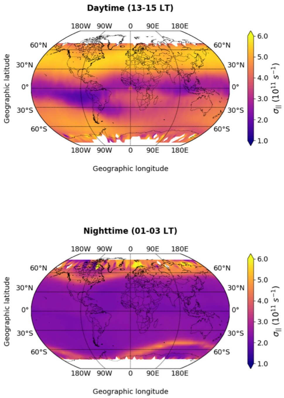
• There is a diurnal variation in ${\sigma }_{\left|\right|}$, due to the diurnal variation in $n_e$ and $T_e$ on which ${\sigma }_{\left|\right|}$ depends;
• In the daytime, ${\sigma }_{\left|\right|}$ is enhanced between ±30° and ±60° latitude and at all longitudes, while it is minimal around the dip equator. The only exception is in correspondence with the South Atlantic region, where an “anomalous” spot of low ${\sigma }_{\left|\right|}$ extends down to about −45° latitude;
• In the daytime, there is a slight hemispheric asymmetry in the ${\sigma }_{\left|\right|}$ values;
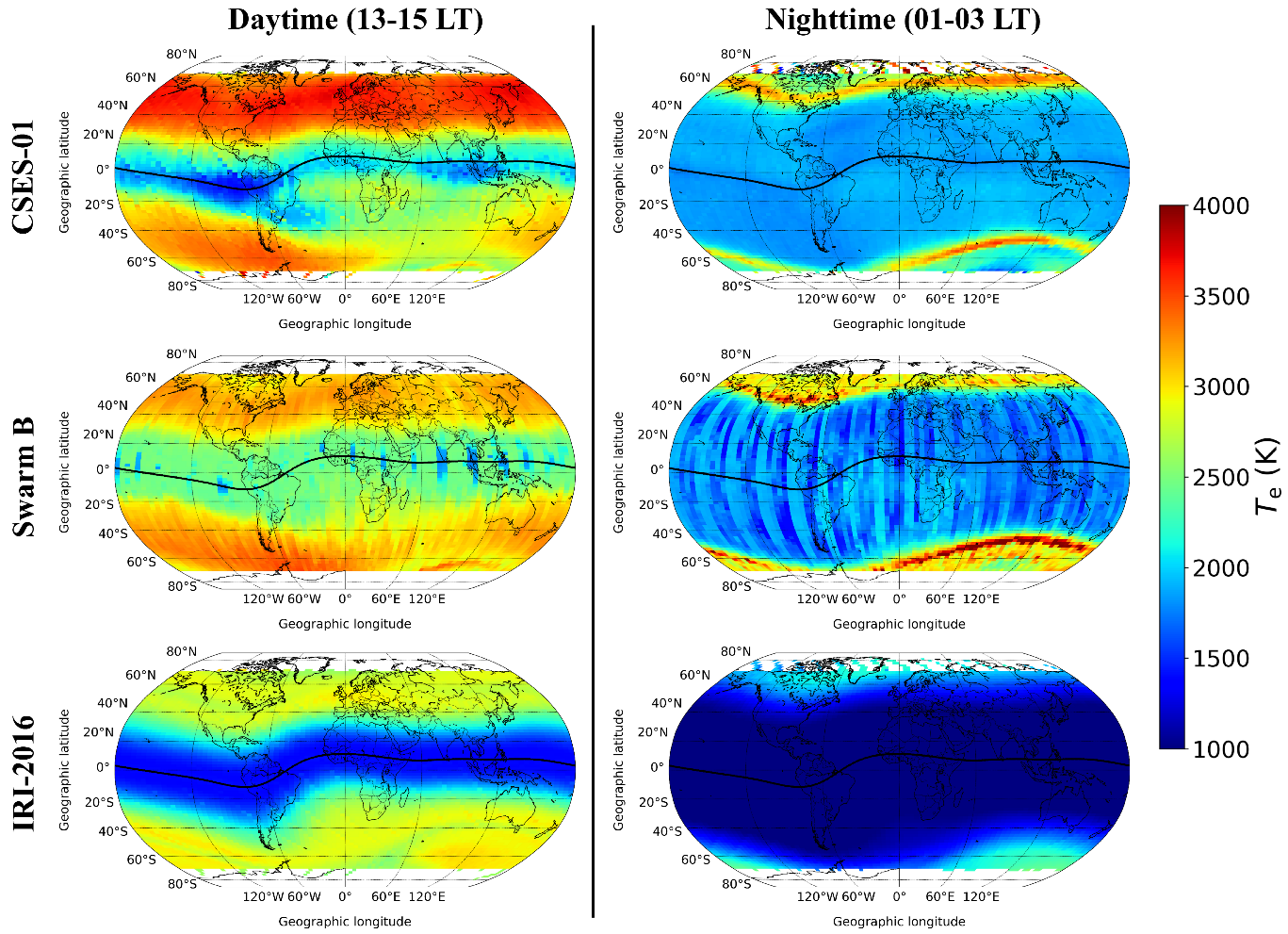
• In the nighttime, the values of ${\sigma }_{\left|\right|}$ are generally low except at subauroral latitudes, i.e., around 60°S and 60°N;
• The features of ${\sigma }_{\left|\right|}$ in the daytime are compatible with the presence of Sq-EEJ current systems;
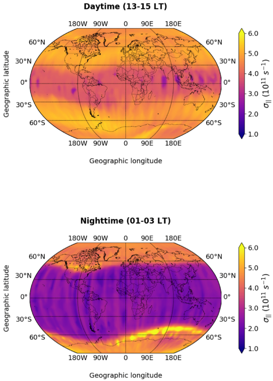
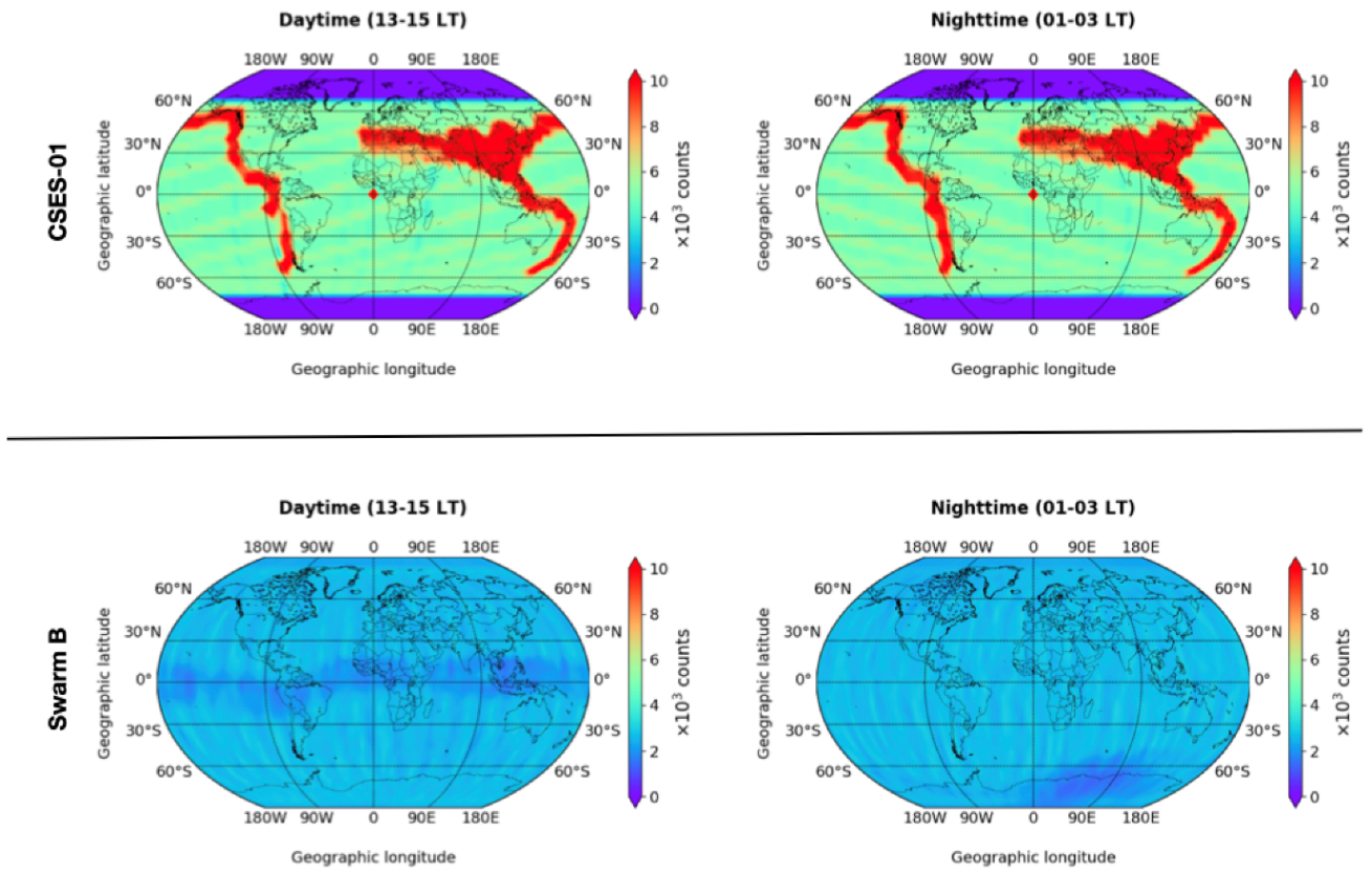
• Results from CSES-01 data are consistent with those from Swarm B, which orbits at a similar altitude. The only difference in the shape of patterns is due to the different statistical coverage of the measurements from the two satellites in the selected time window and at the CSES-01 LTs;
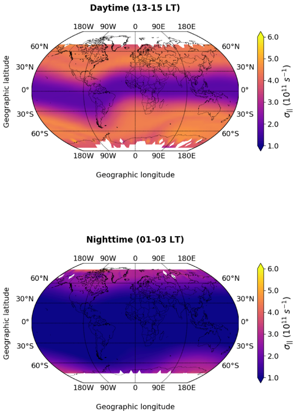
• Both satellites show conductivity values that are generally higher than those expected by ionosphere models such as IRI;
• The study of $T_e$ in the same time window suggests the physical nature of the fine features observed by CSES-01 and the coarse features observed by Swarm B, especially in the daytime. Indeed, $T_e$ features reflect those found in ${\sigma }_{\left|\right|}$.

The results presented in this work are consistent with previous findings concerning certain processes taking place at low and middle latitudes, such as, for example, the presence of a Sq-EEJ current system in the daytime together with the onset of IHFACs connecting hemispheres at specific LTs. However, the future extension of the CSES-01 data set is necessary to highlight both the seasonal and solar/geomagnetic activity dependence of ${\sigma }_{\left|\right|}$. It would also be interesting to investigate the altitude profile of ${\sigma }_{\left|\right|}$, using measurements from other facilities and models of the density and temperature profiles of the various species involved. For these reasons, a more detailed study will follow.

References

- Boteler, D.H.; Pirjola, R.J.; Nevanlinna, H. The effects of geomagnetic disturbances on electrical systems at the Earth’s surface. Adv. Space Res. 1998, 22, 17–27. [Google Scholar] [CrossRef]
- Boteler, D.H.; Pirjola, R.J. Modeling geomagnetically induced currents. Space Weather 2017, 15, 258–276. [Google Scholar] [CrossRef]
- Poedjono, B.; Beck, N.; Buchanan, A.; Borri, L.; Maus, S.; Finn, C.A.; Worthington, E.W.; White, T. Improved Geomagnetic Referencing in the Arctic Environment. Presented at the SPE Arctic and Extreme Environments Technical Conference and Exhibition, Moscow, Russia, 15–17 October 2013. [Google Scholar] [CrossRef]
- Liu, H.; Lühr, H. Strong disturbance of the upper thermospheric density due to magnetic storms: CHAMP observations. J. Geophys. Res. Space Phys. 2005, 110. [Google Scholar] [CrossRef]
- Pirjola, R.; Kauristie, K.; Lappalainen, H.; Viljanen, A.; Pulkkinen, A. Space weather risk. Space Weather 2005, 3. [Google Scholar] [CrossRef]
- Amm, O. Ionospheric Elementary Current Systems in Spherical Coordinates and Their Application. J. Geomagn. Geoelectr. 1997, 49, 947–955. [Google Scholar] [CrossRef]
- Kamide, Y.; Baumjohann, W. Magnetosphere-Ionosphere Coupling; Springer: Berlin/Heidelberg, Germany, 1993; Volume 23. [Google Scholar] [CrossRef]
- Zmuda, A.J.; Martin, J.H.; Heuring, F.T. Transverse magnetic disturbances at 1100 kilometers in the auroral region. J. Geophys. Res. 1966, 71, 5033–5045. [Google Scholar] [CrossRef]
- Zmuda, A.J.; Armstrong, J.C. The diurnal flow pattern of field-aligned currents. J. Geophys. Res. 1974, 79, 4611–4619. [Google Scholar] [CrossRef]
- Iijima, T.; Potemra, T.A. Large-scale characteristics of field-aligned currents associated with substorms. J. Geophys. Res. Space Phys. 1978, 83, 599–615. [Google Scholar] [CrossRef]
- Sugiura, M.; Poros, D.J. An improved model equatorial electrojet with a meridional current system. J. Geophys. Res. Space Phys. 1969, 74, 4025–4034. [Google Scholar] [CrossRef]
- Fambitakoye, O.; Mayaud, P.N. Equatorial electrojet and regular daily variation S/R/. I—A determination of the equatorial electrojet parameters. II—The centre of the equatorial electrojet. J. Atmos. Terr. Phys. 1976, 38, 1–17. [Google Scholar] [CrossRef]
- Mayaud, P. The equatorial counter-electrojet—A review of its geomagnetic aspects. J. Atmos. Terr. Phys. 1977, 39, 1055–1070. [Google Scholar] [CrossRef]
- Marriott, R.; Richmond, A.D.; Venkateswaran, S. The Quiet-Time Equatorial Electrojet and Counter-Electrojet. J. Geomagn. Geoelectr. 1979, 31, 311–340. [Google Scholar] [CrossRef]
- Yamazaki, Y.; Maute, A. Sq and EEJ—A Review on the Daily Variation of the Geomagnetic Field Caused by Ionospheric Dynamo Currents. Space Sci. Rev. 2017, 206, 299–405. [Google Scholar] [CrossRef]
- Maeda, H.; Iyemori, T.; Araki, T.; Kamei, T. New evidence of a meridional current system in the equatorial ionosphere. Geophys. Res. Lett. 1982, 9, 337–340. [Google Scholar] [CrossRef]
- Takeda, M.; Maeda, H. F-region dynamo in the evening - Interpretation of equatorial Delta D anomaly found by MAGSAT. J. Atmos. Terr. Phys. 1983, 45, 401–408. [Google Scholar] [CrossRef]
- Langel, R.A.; Purucker, M.; Rajaram, M. The equatorial electrojet and associated currents as seen in Magsat data. J. Atmos. Terr. Phys. 1993, 55, 1233–1269. [Google Scholar] [CrossRef]
- Van Sabben, D. Magnetospheric currents, associated with the NS asymmetry of Sq. J. Atmos. Terr. Phys. 1966, 28, 965–982. [Google Scholar] [CrossRef]
- Lühr, H.; Kervalishvili, G.; Michaelis, I.; Rauberg, J.; Ritter, P.; Park, J.; Merayo, J.M.G.; Brauer, P. The interhemispheric and F region dynamo currents revisited with the Swarm constellation. Geophys. Res. Lett. 2015, 42, 3069–3075. [Google Scholar] [CrossRef]
- Fukushima, N. Some topics and historical episodes in geomagnetism and aeronomy. J. Geophys. Res. Space Phys. 1994, 99, 19113–19142. [Google Scholar] [CrossRef]
- Olsen, N. Ionospheric F region currents at middle and low latitudes estimated from Magsat data. J. Geophys. Res. Space Phys. 1997, 102, 4563–4576. [Google Scholar] [CrossRef]
- Park, J.; Lühr, H.; Min, K. Climatology of the inter-hemispheric field-aligned current system in the equatorial ionosphere as observed by CHAMP. Ann. Geophys. 2011, 29, 573–582. [Google Scholar] [CrossRef]
- Park, J.; Lühr, H.; Min, K.W. Characteristics of F-region dynamo currents deduced from CHAMP magnetic field measurements. J. Geophys. Res. 2010, 115, A10302. [Google Scholar] [CrossRef]
- Park, J.; Lühr, H.; Fejer, B.G.; Min, K.W. Duskside F-region dynamo currents: Its relationship with prereversal enhancement of vertical plasma drift. Ann. Geophys. 2010, 28, 2097–2101. [Google Scholar] [CrossRef]
- Campbell, W.H. Annual and semiannual variations of the lunar semidiurnal geomagnetic field components at North American locations. J. Geomagn. Geoelectr. 1980, 32, 105–128. [Google Scholar] [CrossRef]
- Maus, S.; Lühr, H. A gravity-driven electric current in the Earth’s ionosphere identified in CHAMP satellite magnetic measurements. Geophys. Res. Lett. 2006, 33, L02812. [Google Scholar] [CrossRef]
- Maute, A.; Richmond, A.D. Examining the Magnetic Signal Due To Gravity and Plasma Pressure Gradient Current With the TIE-GCM. J. Geophys. Res. Space Phys. 2017, 122, 12486–12504. [Google Scholar] [CrossRef]
- Friis-Christensen, E.; Lühr, H.; Hulot, G. SWARM: A constellation to study the Earth’s magnetic field. Earth Planets Space 2006, 58, 351–358. [Google Scholar] [CrossRef]
- Shen, X.; Zhang, X.; Yuan, S.; Wang, L.; Cao, J.; Huang, J.; Zhu, X.; Piergiorgio, P.; Dai, J. The state-of-the-art of the China Seismo-Electromagnetic Satellite mission. Sci. China Technol. Sci. 2018, 61, 634–642. [Google Scholar] [CrossRef]
- Giannattasio, F.; De Michelis, P.; Pignalberi, A.; Coco, I.; Consolini, G.; Pezzopane, M.; Tozzi, R. Parallel Electrical Conductivity in the Topside Ionosphere Derived From Swarm Measurements. J. Geophys. Res. Space Phys. 2021, 126, e2020JA028452. [Google Scholar] [CrossRef]
- Giannattasio, F.; Pignalberi, A.; De Michelis, P.; Coco, I.; Consolini, G.; Pezzopane, M.; Tozzi, R. Dependence of Parallel Electrical Conductivity in the Topside Ionosphere on Solar and Geomagnetic Activity. J. Geophys. Res. Space Phys. 2021, 126, e2021JA029138. [Google Scholar] [CrossRef]
- Rui, Y.; YiBing, G.; XuHui, S.; JianPing, H.; XueMin, Z.; Chao, L.; Liu, D. The Langmuir Probe onboard CSES: Data inversion analysis method and first results. Earth Planet. Phys. 2018, 2, 479. [Google Scholar] [CrossRef]
- Liu, C.; Yibing, G.; Zheng, X.; Aibing, Z.; Diego, P.; Sun, Y. The technology of space plasma in situ measurement on the China Seismo-Electromagnetic Satellite. Sci. China Technol. Sci. 2018, 62, 829–838. [Google Scholar] [CrossRef]
- Yan, R.; Guan, Y.; Miao, Y.; Zhima, Z.; Xiong, C.; Zhu, X.; Liu, C.; Shen, X.; Yuan, S.; Liu, D.; et al. The Regular Features Recorded by the Langmuir Probe Onboard the Low Earth Polar Orbit Satellite CSES. J. Geophys. Res. Space Phys. 2022, 127, e2021JA029289. [Google Scholar] [CrossRef]
- Knudsen, D.J.; Burchill, J.K.; Buchert, S.C.; Eriksson, A.I.; Gill, R.; Wahlund, J.; Åhlen, L.; Smith, M.; Moffat, B. Thermal ion imagers and Langmuir probes in the Swarm electric field instruments. J. Geophys. Res. Space Phys. 2017, 122, 2655–2673. [Google Scholar] [CrossRef]
- Kelley, M. The Earth’s Ionosphere: Plasma Physics and Electrodynamics; Elsevier Science: Amsterdam, The Netherlands, 2009. [Google Scholar]
- Moen, J.; Brekke, A. On the importance of ion composition to conductivities in the auroral ionosphere. J. Geophys. Res. Space Phys. 1990, 95, 10687–10693. [Google Scholar] [CrossRef]
- Moen, J.; Brekke, A. The solar flux influence on quiet time conductances in the auroral ionosphere. Geophys. Res. Lett. 1993, 20, 971–974. [Google Scholar] [CrossRef]
- Rishbeth, H. The ionospheric E-layer and F-layer dynamos—A tutorial review. J. Atmos. Sol.-Terr. Phys. 1997, 59, 1873–1880. [Google Scholar] [CrossRef]
- Cravens, T.E.; Dessler, A.J.; Houghton, J.T.; Rycroft, M.J. Physics of Solar System Plasmas; Cambridge University Press: Cambridge, UK, 1997. [Google Scholar]
- Aggarwal, K.; Nath, N.; Setty, C. Collision frequency and transport properties of electrons in the ionosphere. Planet. Space Sci. 1979, 27, 753–768. [Google Scholar] [CrossRef]
- Vickrey, J.F.; Vondrak, R.R.; Matthews, S.J. The diurnal and latitudinal variation of auroral zone ionospheric conductivity. J. Geophys. Res. Space Phys. 1981, 86, 65–75. [Google Scholar] [CrossRef]
- Nicolet, M. The collision frequency of electrons in the ionosphere. J. Atmos. Terr. Phys. 1953, 3, 200–211. [Google Scholar] [CrossRef]
- Singh, R.N. The effective electron collision frequency in the lower F region of the ionosphere. Proc. Phys. Soc. 1966, 87, 425–428. [Google Scholar] [CrossRef]
- Takeda, M.; Araki, T. Electric conductivity of the ionosphere and nocturnal currents. J. Atmos. Terr. Phys. 1985, 47, 601–609. [Google Scholar] [CrossRef]
- Nishino, M.; Nozawa, S.; Holtet, J.A. Daytime ionospheric absorption features in the polar cap associated with poleward drifting F-region plasma patches. Earth Planets Space 1998, 50, 107–117. [Google Scholar] [CrossRef]
- Lomidze, L.; Knudsen, D.J.; Burchill, J.; Kouznetsov, A.; Buchert, S.C. Calibration and Validation of Swarm Plasma Densities and Electron Temperatures Using Ground-Based Radars and Satellite Radio Occultation Measurements. Radio Sci. 2018, 53, 15–36. [Google Scholar] [CrossRef]
- Pezzopane, M.; Pignalberi, A.; De Michelis, P.; Consolini, G.; Coco, I.; Giannattasio, F.; Tozzi, R.; Zoffoli, S. On the best settings to calculate ionospheric irregularities indices from the in situ plasma parameters of CSES-01. IEEE J. Sel. Top. Appl. Earth Obs. Remote Sens. 2022, 15, 4058–4071. [Google Scholar] [CrossRef]
- Chapman, S. The electrical conductivity of the ionosphere: A review. Il Nuovo Cimento 1956, 4, 1385–1412. [Google Scholar] [CrossRef]
- Schunk, R.W.; Nagy, A.F. Electron temperatures in the F region of the ionosphere: Theory and observations. Rev. Geophys. 1978, 16, 355–399. [Google Scholar] [CrossRef]
- McDonald, J.; Williams, P. The relationship between ionospheric temperature, electron density and solar activity. J. Atmos. Terr. Phys. 1980, 42, 41–44. [Google Scholar] [CrossRef]
- Prölss, G.W. Subauroral electron temperature enhancement in the nighttime ionosphere. Ann. Geophys. 2006, 24, 1871–1885. [Google Scholar] [CrossRef]
- Wang, W.; Burns, A.G.; Killeen, T.L. A numerical study of the response of ionospheric electron temperature to geomagnetic activity. J. Geophys. Res. Space Phys. 2006, 111. [Google Scholar] [CrossRef]
- Bilitza, D.; Altadill, D.; Truhlik, V.; Shubin, V.; Galkin, I.; Reinisch, B.; Huang, X. International Reference Ionosphere 2016: From ionospheric climate to real-time weather predictions. Space Weather 2017, 15, 418–429. [Google Scholar] [CrossRef]
- Bilitza, D. IRI the International Standard for the Ionosphere. Adv. Radio Sci. 2018, 16, 1–11. [Google Scholar] [CrossRef]
- Nava, B.; Coïsson, P.; Radicella, S. A new version of the NeQuick ionosphere electron density model. J. Atmos. Sol.-Terr. Phys. 2008, 70, 1856–1862. [Google Scholar] [CrossRef]
- Coïsson, P.; Nava, B.; Radicella, S.M. On the use of NeQuick topside option in IRI-2007. Adv. Space Res. 2009, 43, 1688–1693. [Google Scholar] [CrossRef]
- Pignalberi, A.; Pezzopane, M.; Tozzi, R.; De Michelis, P.; Coco, I. Comparison between IRI and preliminary Swarm Langmuir probe measurements during the St. Patrick storm period. Earth Planets Space 2016, 68, 93. [Google Scholar] [CrossRef]
- Pignalberi, A.; Pezzopane, M.; Themens, D.R.; Haralambous, H.; Nava, B.; Coïsson, P. On the Analytical Description of the Topside Ionosphere by NeQuick: Modeling the Scale Height Through COSMIC/FORMOSAT-3 Selected Data. IEEE J. Sel. Top. Appl. Earth Obs. Remote Sens. 2020, 13, 1867–1878. [Google Scholar] [CrossRef]
- Truhlik, V.; Bilitza, D.; Triskova, L. A new global empirical model of the electron temperature with the inclusion of the solar activity variations for IRI. Earth Planets Space 2012, 64, 531–543. [Google Scholar] [CrossRef]
- Shim, J.S.; Kuznetsova, M.; Rastätter, L.; Hesse, M.; Bilitza, D.; Butala, M.; Codrescu, M.; Emery, B.; Foster, B.; Fuller-Rowell, T.; et al. CEDAR Electrodynamics Thermosphere Ionosphere (ETI) Challenge for systematic assessment of ionosphere/thermosphere models: NmF2, hmF2, and vertical drift using ground-based observations. Space Weather 2011, 9. [Google Scholar] [CrossRef]
- Shim, J.S.; Kuznetsova, M.; Rastätter, L.; Bilitza, D.; Butala, M.; Codrescu, M.; Emery, B.A.; Foster, B.; Fuller-Rowell, T.J.; Huba, J.; et al. CEDAR Electrodynamics Thermosphere Ionosphere (ETI) Challenge for systematic assessment of ionosphere/thermosphere models: Electron density, neutral density, NmF2, and hmF2 using space based observations. Space Weather 2012, 10. [Google Scholar] [CrossRef]
- Tsagouri, I.; Goncharenko, L.; Shim, J.S.; Belehaki, A.; Buresova, D.; Kuznetsova, M.M. Assessment of Current Capabilities in Modeling the Ionospheric Climatology for Space Weather Applications: FoF2 and hmF2. Space Weather 2018, 16, 1930–1945. [Google Scholar] [CrossRef]
- Themens, D.R.; Jayachandran, P.T.; Galkin, I.; Hall, C. The Empirical Canadian High Arctic Ionospheric Model (E-CHAIM): NmF2 and hmF2. J. Geophys. Res. Space Phys. 2017, 122, 9015–9031. [Google Scholar] [CrossRef]
- Consolini, G.; Quattrociocchi, V.; D’Angelo, G.; Alberti, T.; Piersanti, M.; Marcucci, M.F.; De Michelis, P. Electric Field Multifractal Features in the High-Latitude Ionosphere: CSES-01 Observations. Atmosphere 2021, 12, 646. [Google Scholar] [CrossRef]
- Takeda, M. Time variation of global geomagnetic Sq field in 1964 and 1980. J. Atmos. Sol.-Terr. Phys. 1999, 61, 765–774. [Google Scholar] [CrossRef]
- Çelik, C. The lunar daily geomagnetic variation and its dependence on sunspot number. J. Atmos. Sol.-Terr. Phys. 2014, 119, 153–161. [Google Scholar] [CrossRef]
- Takeda, M. Geomagnetic field variation and the equivalent current system generated by an ionospheric dynamo at the solstice. J. Atmos. Terr. Phys. 1990, 52, 59–67. [Google Scholar] [CrossRef]
- Heelis, R.A.; Coley, W.R.; Burrell, A.G.; Hairston, M.R.; Earle, G.D.; Perdue, M.D.; Power, R.A.; Harmon, L.L.; Holt, B.J.; Lippincott, C.R. Behavior of the O+/H+ transition height during the extreme solar minimum of 2008. Geophys. Res. Lett. 2009, 36. [Google Scholar] [CrossRef]
- Klenzing, J.; Simoes, F.; Ivanov, S.; Heelis, R.A.; Bilitza, D.; Pfaff, R.; Rowland, D. Topside equatorial ionospheric density and composition during and after extreme solar minimum. J. Geophys. Res. Space Phys. 2011, 116. [Google Scholar] [CrossRef]
- Klenzing, J.; Burrell, A.G.; Heelis, R.A.; Huba, J.D.; Pfaff, R.; Simões, F. Exploring the role of ionospheric drivers during the extreme solar minimum of 2008. Ann. Geophys. 2013, 31, 2147–2156. [Google Scholar] [CrossRef]
- Huba, J.D.; Heelis, R.; Maute, A. Large-Scale O+ Depletions Observed by ICON in the Post-Midnight Topside Ionosphere: Data/Model Comparison. Geophys. Res. Lett. 2021, 48, e2020GL092061. [Google Scholar] [CrossRef]
- Debchoudhury, S.; Barjatya, A.; Minow, J.I.; Coffey, V.N.; Parker, L.N. Climatology of Deep O+ Dropouts in the Night-Time F-Region in Solar Minimum Measured by a Langmuir Probe Onboard the International Space Station. J. Geophys. Res. Space Phys. 2022, 127, e2022JA030446. [Google Scholar] [CrossRef]
- Vaishnav, R.; Jin, Y.; Mostafa, M.G.; Aziz, S.R.; Zhang, S.R.; Jacobi, C. Study of the upper transition height using ISR observations and IRI predictions over Arecibo. Adv. Space Res. 2021, 68, 2177–2185. [Google Scholar] [CrossRef]
- Pignalberi, A.; Giannattasio, F.; Truhlik, V.; Coco, I.; Pezzopane, M.; Consolini, G.; De Michelis, P.; Tozzi, R. On the Electron Temperature in the Topside Ionosphere as Seen by Swarm Satellites, Incoherent Scatter Radars, and the International Reference Ionosphere Model. Remote Sens. 2021, 13, 4077. [Google Scholar] [CrossRef]
- Willmore, A.P.; Massey, H.S.W. Geographical and solar activity variations in the electron temperature of the upper F region. Proc. R. Soc. Lond. Ser. A Math. Phys. Sci. 1965, 286, 537–558. [Google Scholar] [CrossRef]
- Gledhill, J.A. Aeronomic effects of the South Atlantic anomaly. Rev. Geophys. Space Phys. 1976, 14, 173–187. [Google Scholar] [CrossRef]
- Hirao, K.; Oyama, K. Local characteristics of the electron temperature profile. J. Geomagn. Geoelectr. 1976, 28, 507–514. [Google Scholar] [CrossRef]
- Oyama, K.; Schlegel, K. Anomalous electron temperatures above the South American magnetic field anomaly. Planet. Space Sci. 1984, 32, 1513–1522. [Google Scholar] [CrossRef]
- Horvath, I.; Lovell, B.C. Investigating the relationships among the South Atlantic Magnetic Anomaly, southern nighttime midlatitude trough, and nighttime Weddell Sea Anomaly during southern summer. J. Geophys. Res. (Space Phys.) 2009, 114, A02306. [Google Scholar] [CrossRef]
Publisher’s Note: MDPI stays neutral with regard to jurisdictional claims in published maps and institutional affiliations. |
© 2022 by the authors. Licensee MDPI, Basel, Switzerland. This article is an open access article distributed under the terms and conditions of the Creative Commons Attribution (CC BY) license (https://creativecommons.org/licenses/by/4.0/).
Share and Cite
Giannattasio, F.; Pignalberi, A.; De Michelis, P.; Coco, I.; Pezzopane, M.; Tozzi, R.; Consolini, G. Parallel Electrical Conductivity at Low and Middle Latitudes in the Topside Ionosphere Derived from CSES-01 Measurements. Remote Sens. 2022, 14, 5079. https://doi.org/10.3390/rs14205079
Giannattasio F, Pignalberi A, De Michelis P, Coco I, Pezzopane M, Tozzi R, Consolini G. Parallel Electrical Conductivity at Low and Middle Latitudes in the Topside Ionosphere Derived from CSES-01 Measurements. Remote Sensing. 2022; 14(20):5079. https://doi.org/10.3390/rs14205079
Chicago/Turabian StyleGiannattasio, Fabio, Alessio Pignalberi, Paola De Michelis, Igino Coco, Michael Pezzopane, Roberta Tozzi, and Giuseppe Consolini. 2022. "Parallel Electrical Conductivity at Low and Middle Latitudes in the Topside Ionosphere Derived from CSES-01 Measurements" Remote Sensing 14, no. 20: 5079. https://doi.org/10.3390/rs14205079
APA StyleGiannattasio, F., Pignalberi, A., De Michelis, P., Coco, I., Pezzopane, M., Tozzi, R., & Consolini, G. (2022). Parallel Electrical Conductivity at Low and Middle Latitudes in the Topside Ionosphere Derived from CSES-01 Measurements. Remote Sensing, 14(20), 5079. https://doi.org/10.3390/rs14205079