Figure 1.
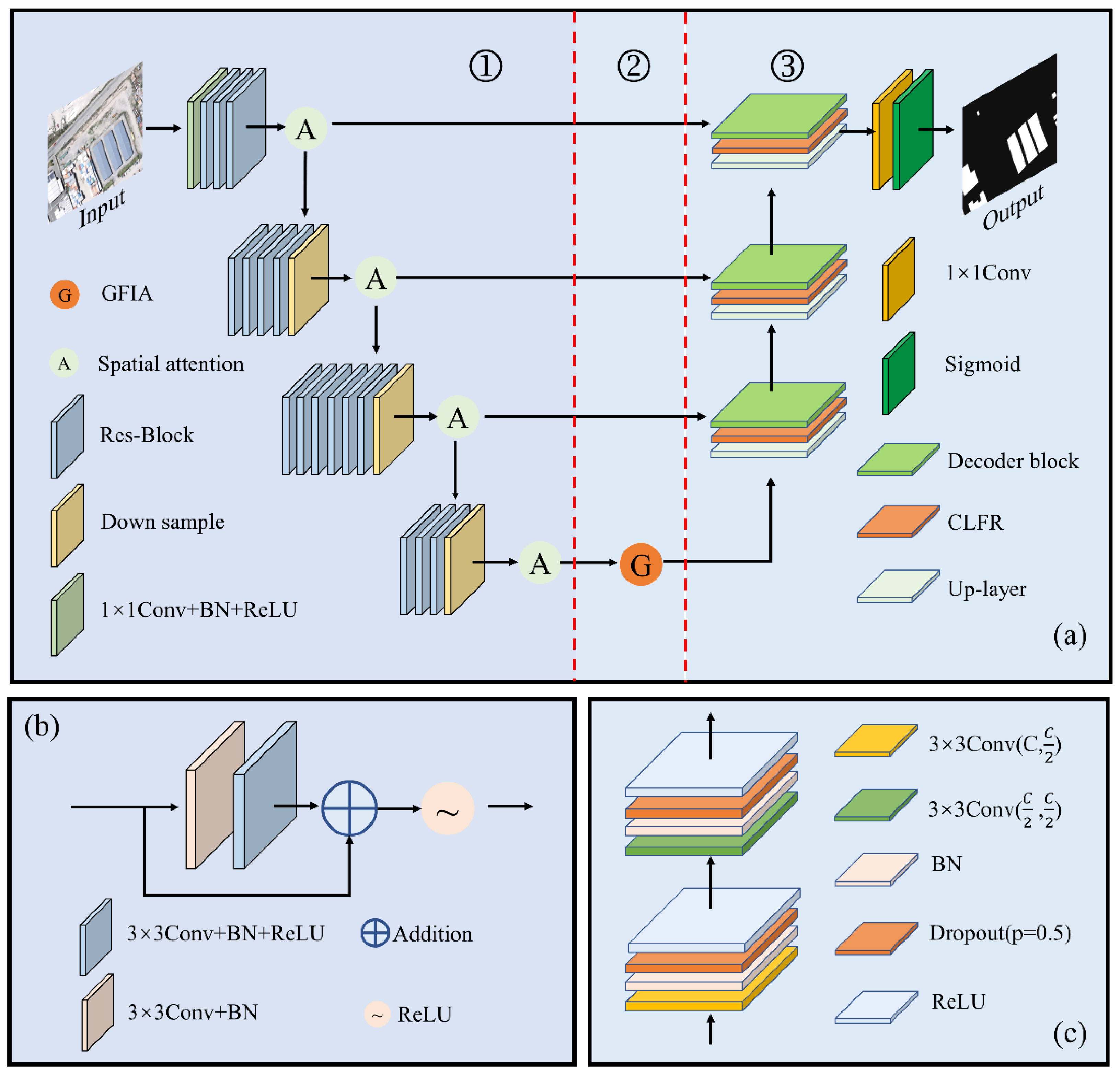
Overall of the proposed framework. (a) Structure of the B-FGC-Net, in which ①, ②, and ③ denote the encoder, the GFIA module, and the decoder, respectively, Down sample denotes downsampling, Up-layer denotes upsampling; (b) Res-Block; (c) Decoder-Block, where C denotes the number of channels of the feature map, and p is the probability of an element being zeroed. The addition and ReLU represent the pixel addition and the Rectified Linear Unit, respectively. The 1 × 1 and 3 × 3 denote the convolution kernel size.
Figure 2.
The structure of the spatial attention unit.
Figure 2.
The structure of the spatial attention unit.
Figure 3.
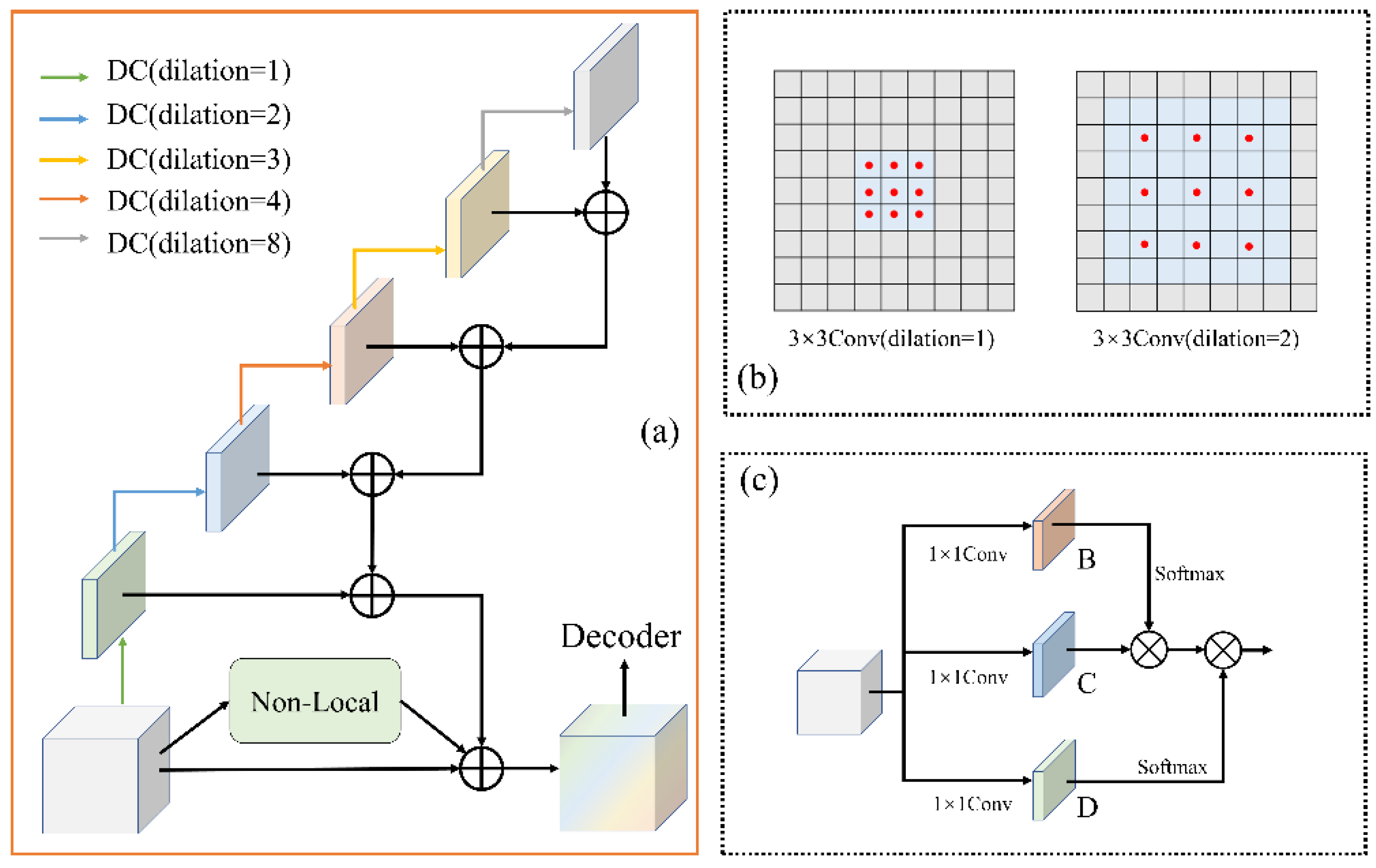
Overview of the GFIA module. (a) The structure of the GFIA module, (b) the comparison of standard convolution and dilated convolution, (c) the structure of the nonlocal units.
Figure 3.
Overview of the GFIA module. (a) The structure of the GFIA module, (b) the comparison of standard convolution and dilated convolution, (c) the structure of the nonlocal units.
Figure 4.
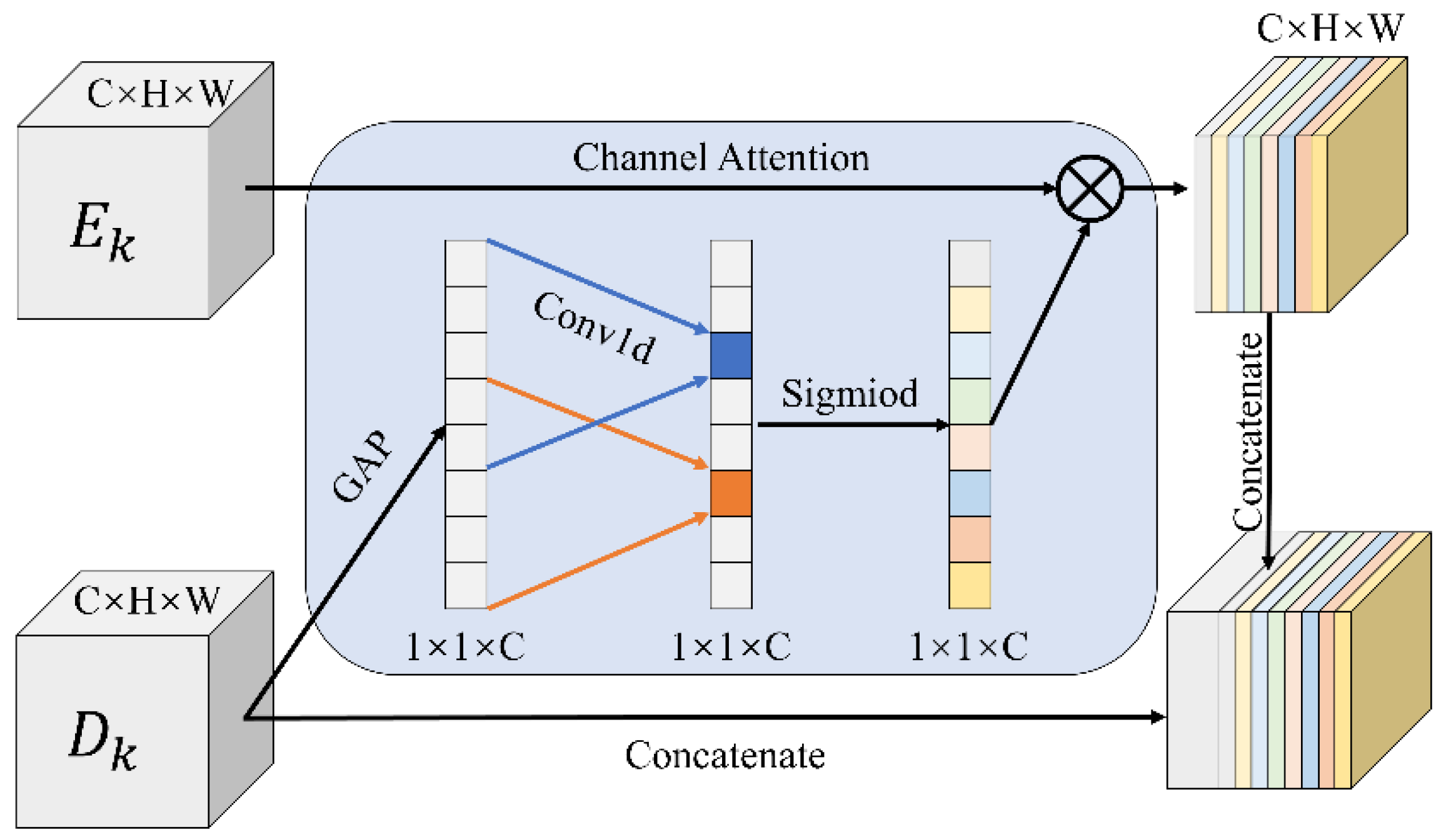
The structure of the CLFR module.
Figure 4.
The structure of the CLFR module.
Figure 5.
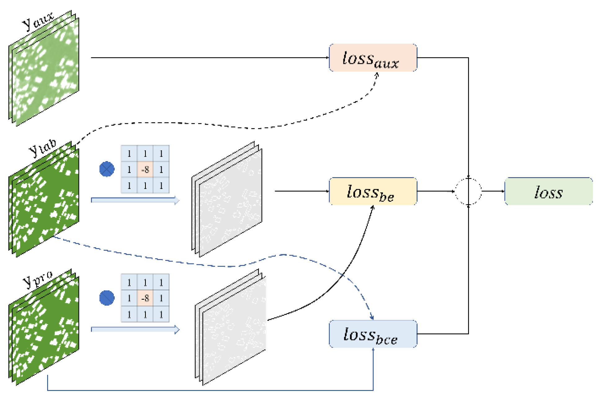
Flow chart of the loss function. The 3 × 3 matrix represents the Laplacian operator.
Figure 5.
Flow chart of the loss function. The 3 × 3 matrix represents the Laplacian operator.
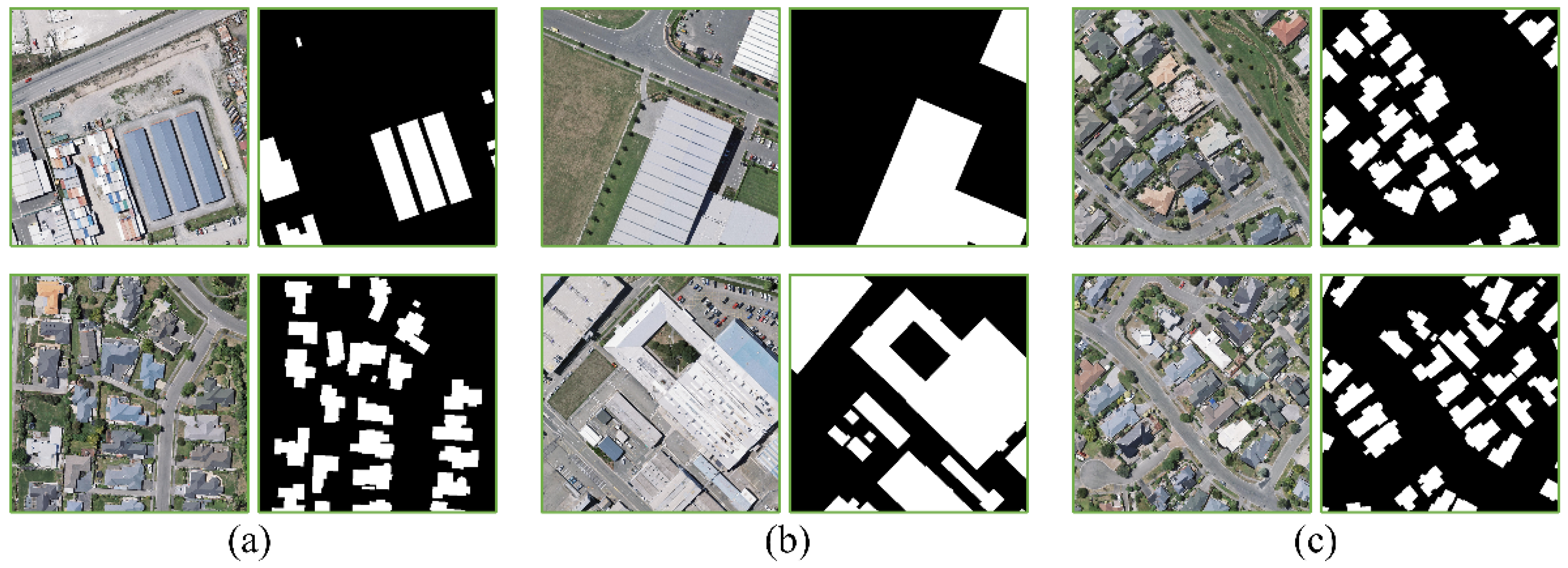
Figure 6.
Examples of the original images and the ground truth of the WHU building dataset. (a–c) are training, validation, and testing samples, respectively.
Figure 6.
Examples of the original images and the ground truth of the WHU building dataset. (a–c) are training, validation, and testing samples, respectively.
Figure 7.
Examples of the images and the ground truth of the INRIA aerial image labeling dataset. (a,b) are the original dataset and the preprocessed image examples, respectively.
Figure 7.
Examples of the images and the ground truth of the INRIA aerial image labeling dataset. (a,b) are the original dataset and the preprocessed image examples, respectively.
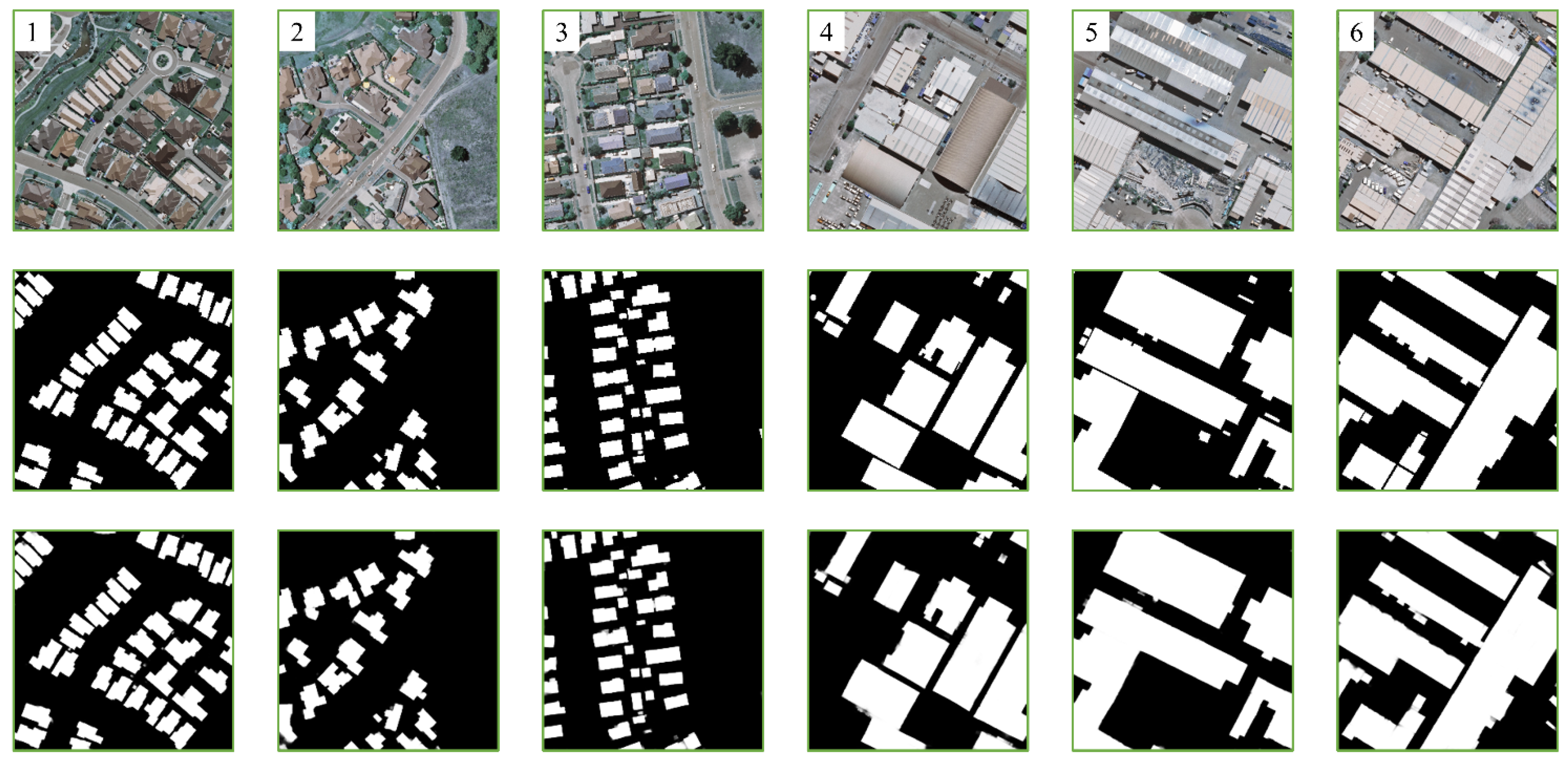
Figure 8.
Building extraction results of the B-FGC-Net on the WHU building dataset. The first to third rows are the original images, labels, and results, respectively. The numbers 1–6 represent the index in which the image is located.
Figure 8.
Building extraction results of the B-FGC-Net on the WHU building dataset. The first to third rows are the original images, labels, and results, respectively. The numbers 1–6 represent the index in which the image is located.
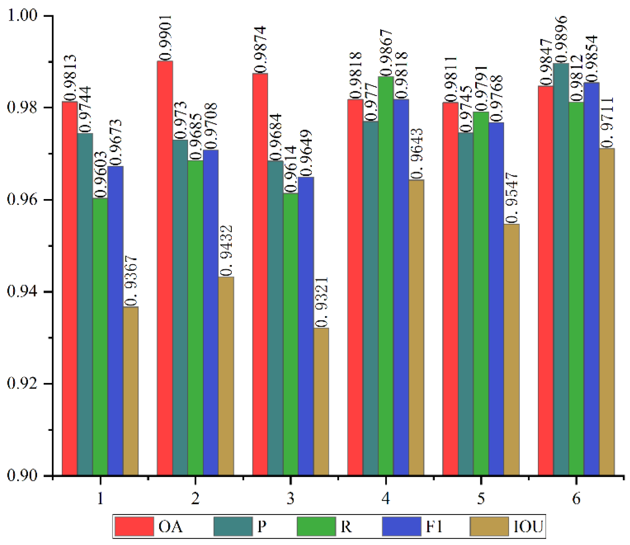
Figure 9.
Evaluation results on the WHU building dataset.
Figure 9.
Evaluation results on the WHU building dataset.
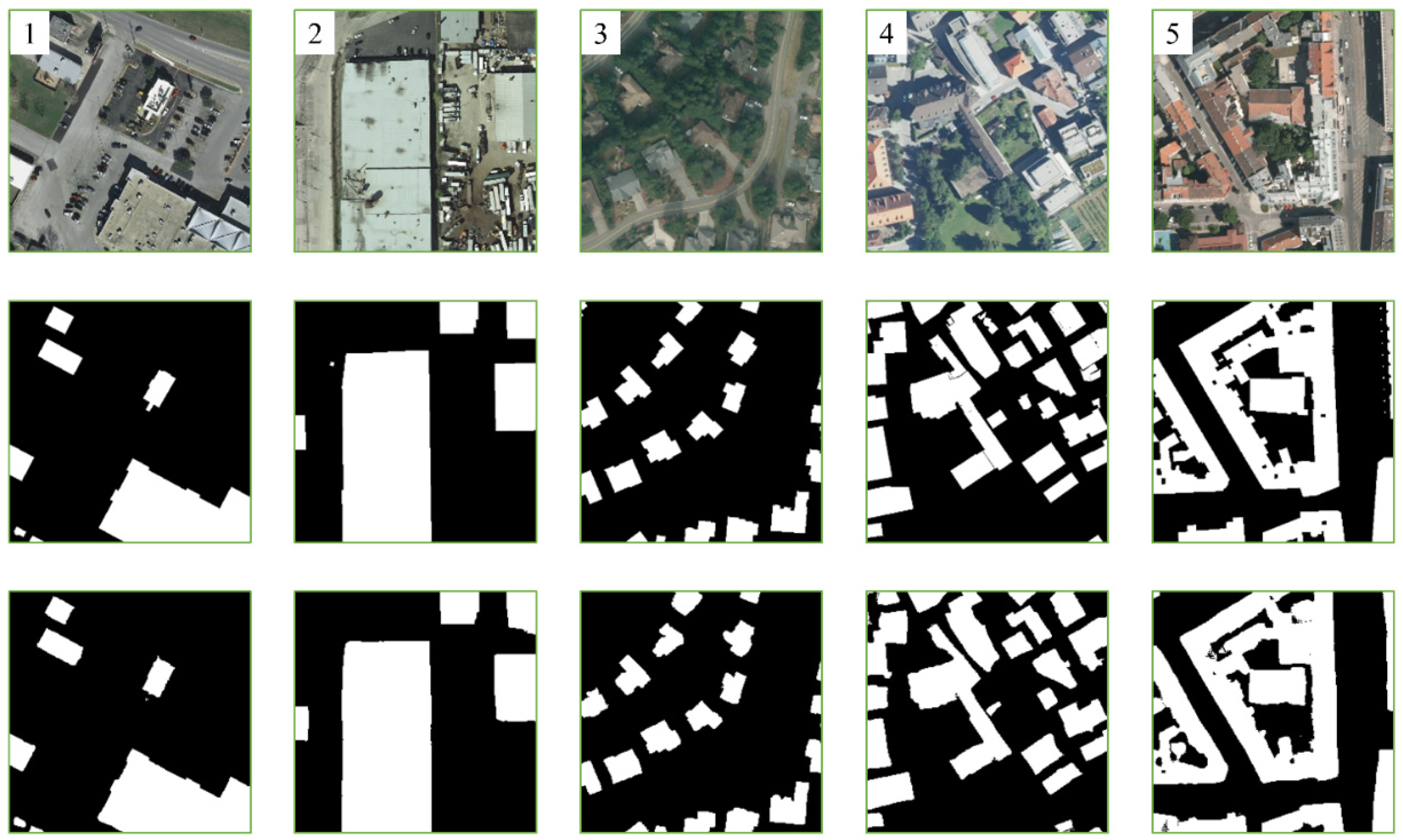
Figure 10.
The extraction results of B-FGC-Net on the INRIA aerial image labeling dataset. The first to third rows are the test images, labels, and results, respectively. Numbers 1–5 represent Austin, Chicago, Kitsap County, West Tyrol, and Vienna, respectively.
Figure 10.
The extraction results of B-FGC-Net on the INRIA aerial image labeling dataset. The first to third rows are the test images, labels, and results, respectively. Numbers 1–5 represent Austin, Chicago, Kitsap County, West Tyrol, and Vienna, respectively.
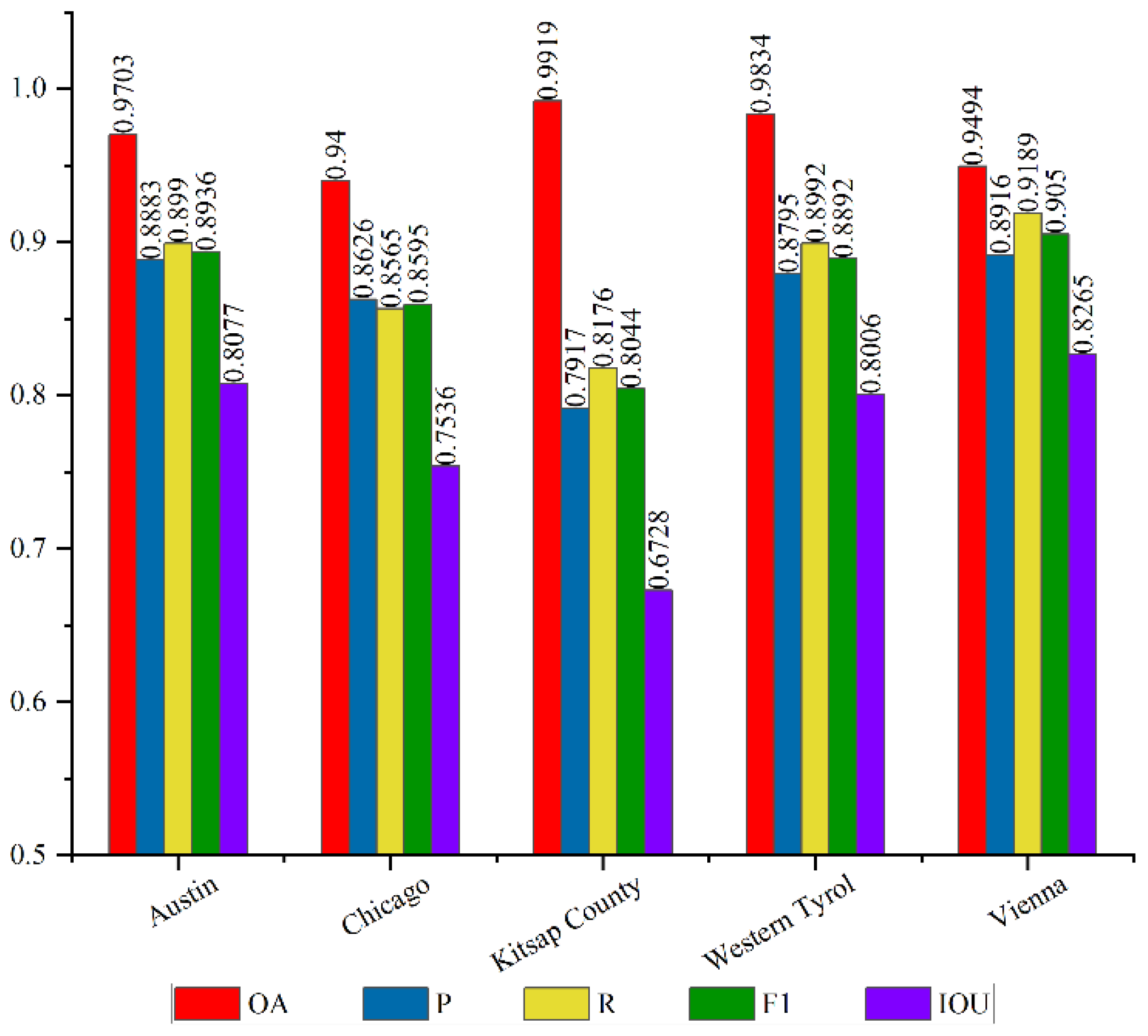
Figure 11.
Evaluation results on the Inria Aerial Image Labeling dataset.
Figure 11.
Evaluation results on the Inria Aerial Image Labeling dataset.
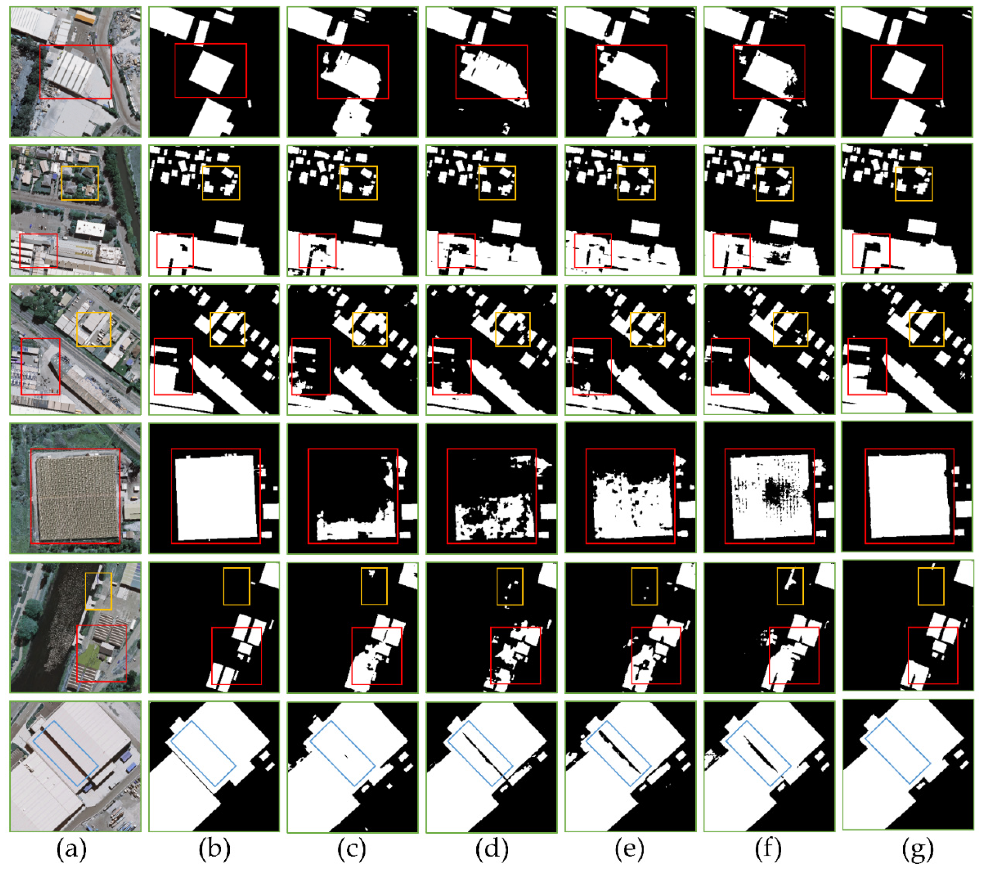
Figure 12.
Extraction results of different models on the WHU Building Dataset. (a) Original image, (b) label, (c) U-Net, (d) Res-UNet, (e) LinkNet, (f) LinkNet*, (g) B-FGC-Net.
Figure 12.
Extraction results of different models on the WHU Building Dataset. (a) Original image, (b) label, (c) U-Net, (d) Res-UNet, (e) LinkNet, (f) LinkNet*, (g) B-FGC-Net.
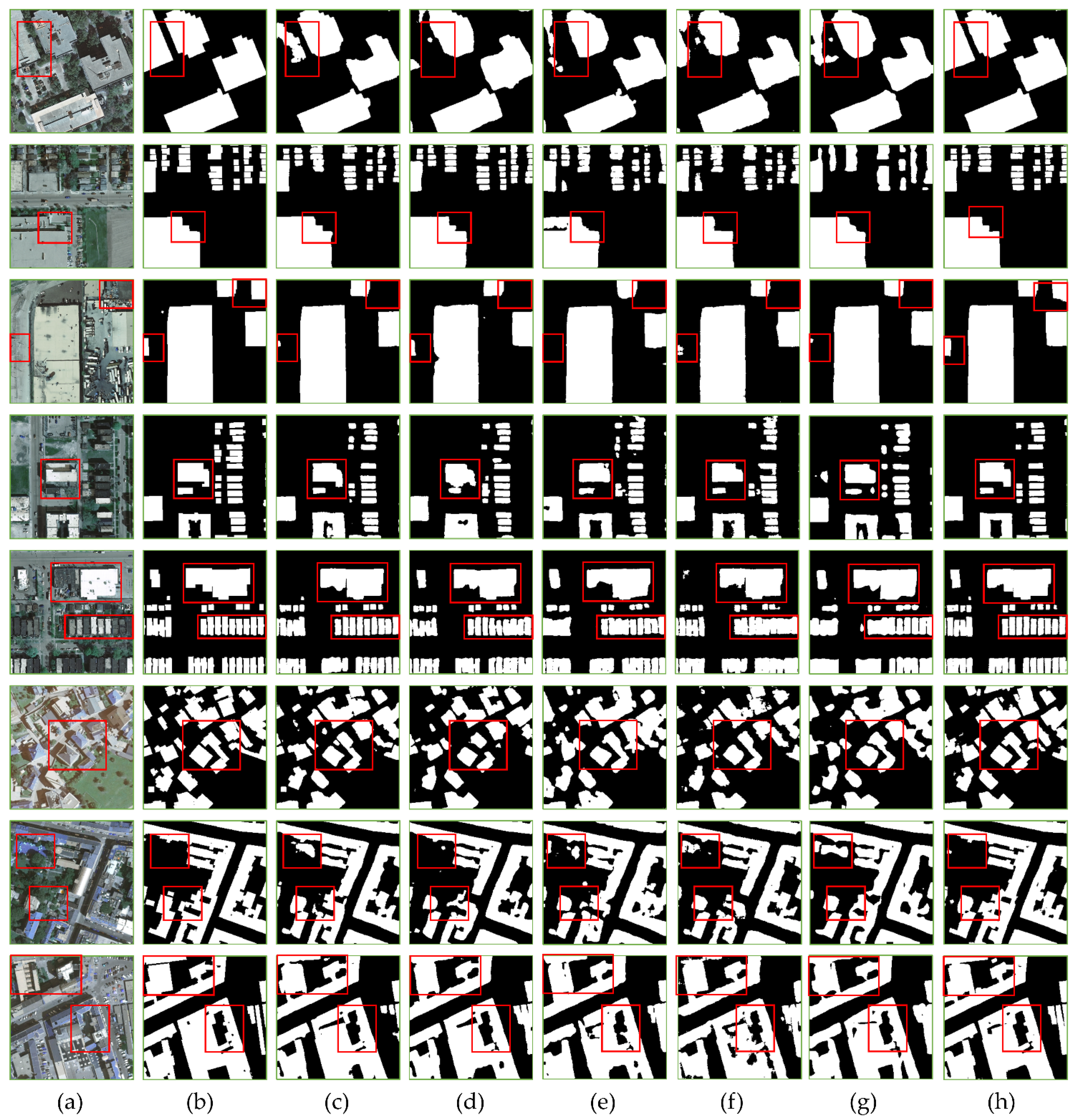
Figure 13.
The extraction results of different methods on the INRIA aerial image labeling dataset. (a) Original images, (b) labels, (c) U-Net, (d) Res-UNet, (e) LinkNet, (f) SegNet, (g) DeepLabV3, (h) B-FGC-Net.
Figure 13.
The extraction results of different methods on the INRIA aerial image labeling dataset. (a) Original images, (b) labels, (c) U-Net, (d) Res-UNet, (e) LinkNet, (f) SegNet, (g) DeepLabV3, (h) B-FGC-Net.
Figure 14.
Visualization results of different levels of SA: (a) original images, (b,c) before and after SA_1, (d,e) before and after SA_2, (f,g) before and after SA_3, (h,i) before and after SA_4.
Figure 14.
Visualization results of different levels of SA: (a) original images, (b,c) before and after SA_1, (d,e) before and after SA_2, (f,g) before and after SA_3, (h,i) before and after SA_4.
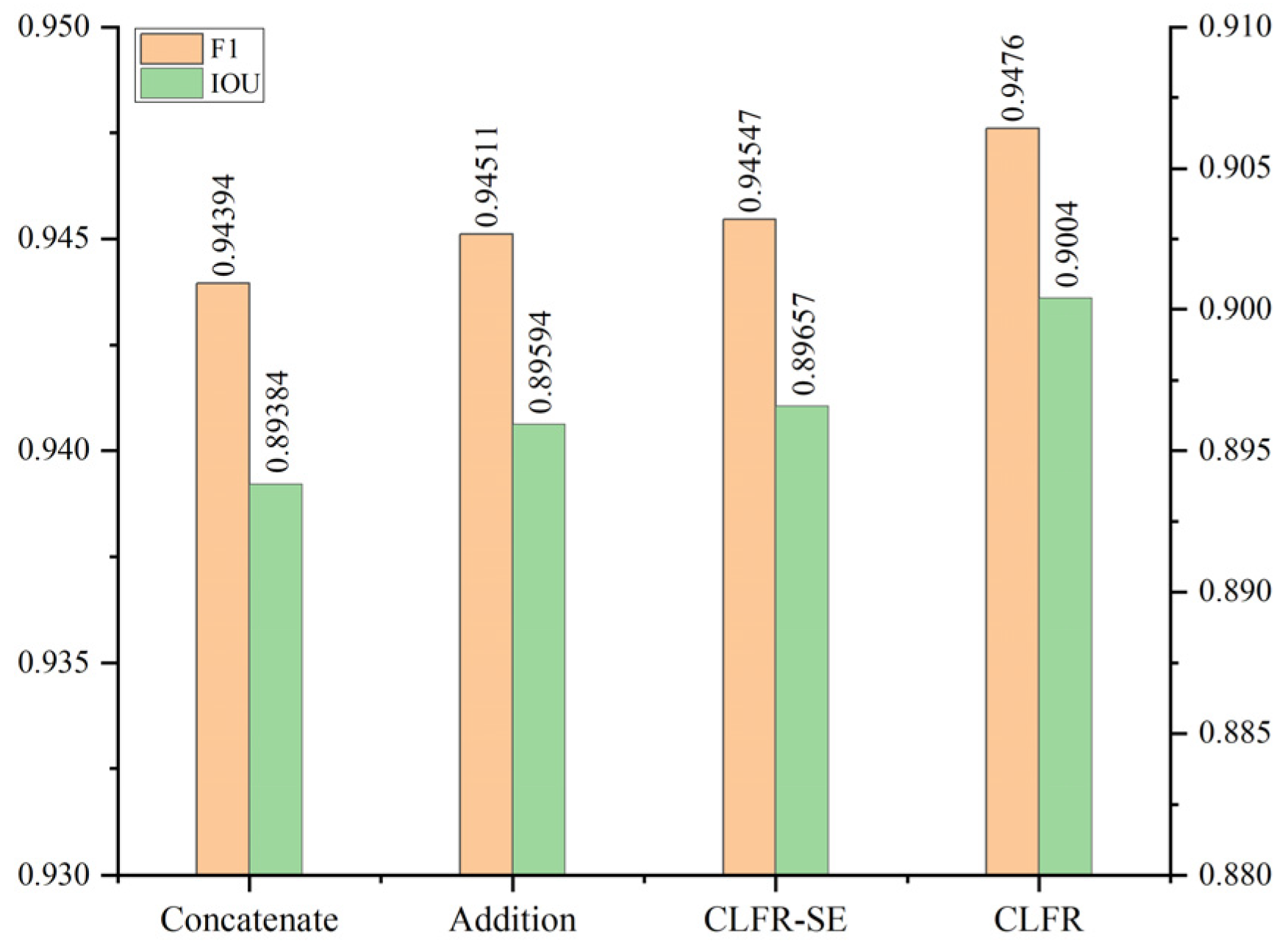
Figure 15.
F1 scores and IOU of different cross level feature fusion schemes on the WHU building dataset.
Figure 15.
F1 scores and IOU of different cross level feature fusion schemes on the WHU building dataset.
Figure 16.
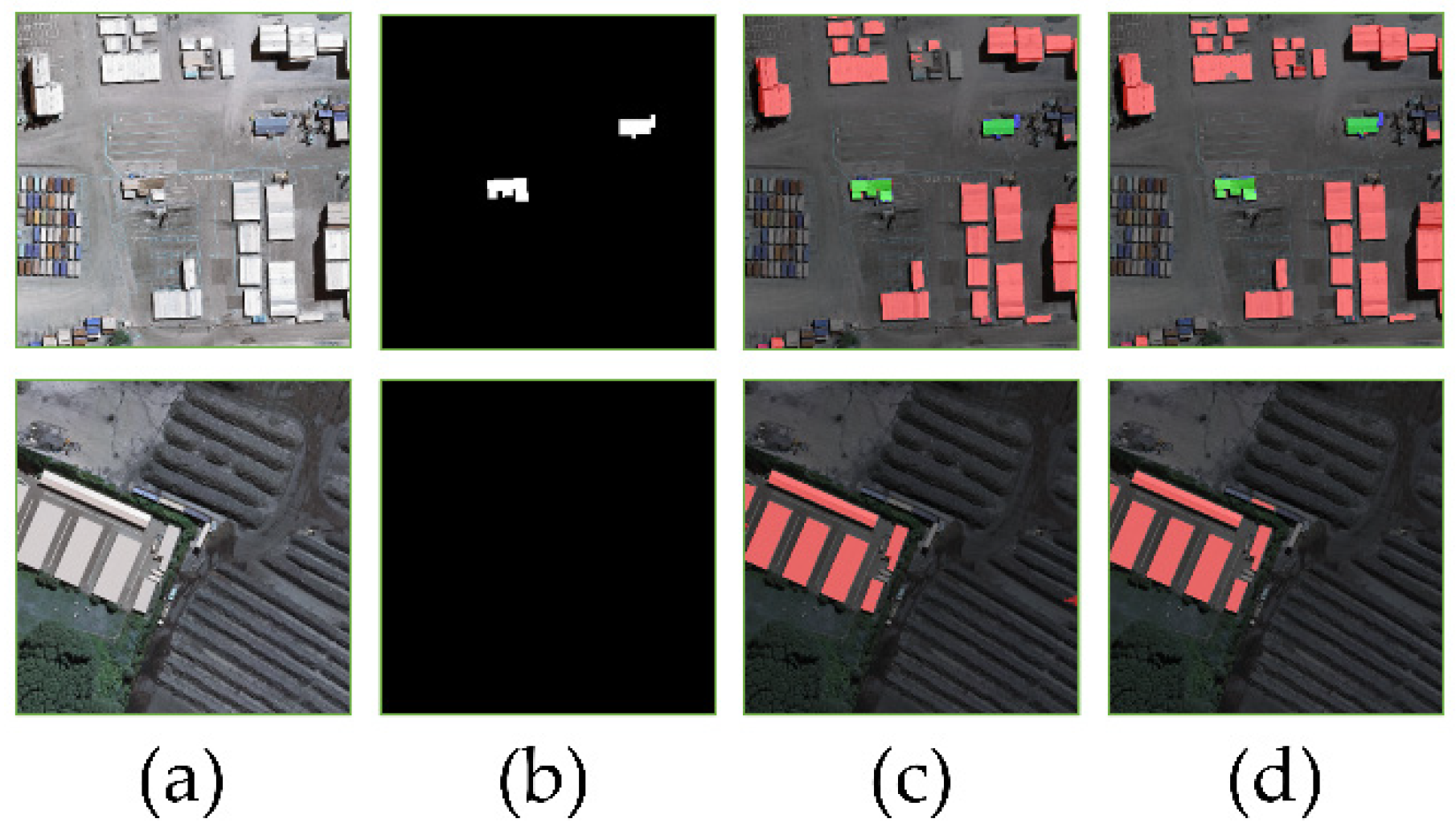
Examples of error extraction. (a) Original images, (b) labels, (c) U-Net, (d) B-FGC-Net. The green and red indicate the correct and incorrect, respectively.
Figure 16.
Examples of error extraction. (a) Original images, (b) labels, (c) U-Net, (d) B-FGC-Net. The green and red indicate the correct and incorrect, respectively.
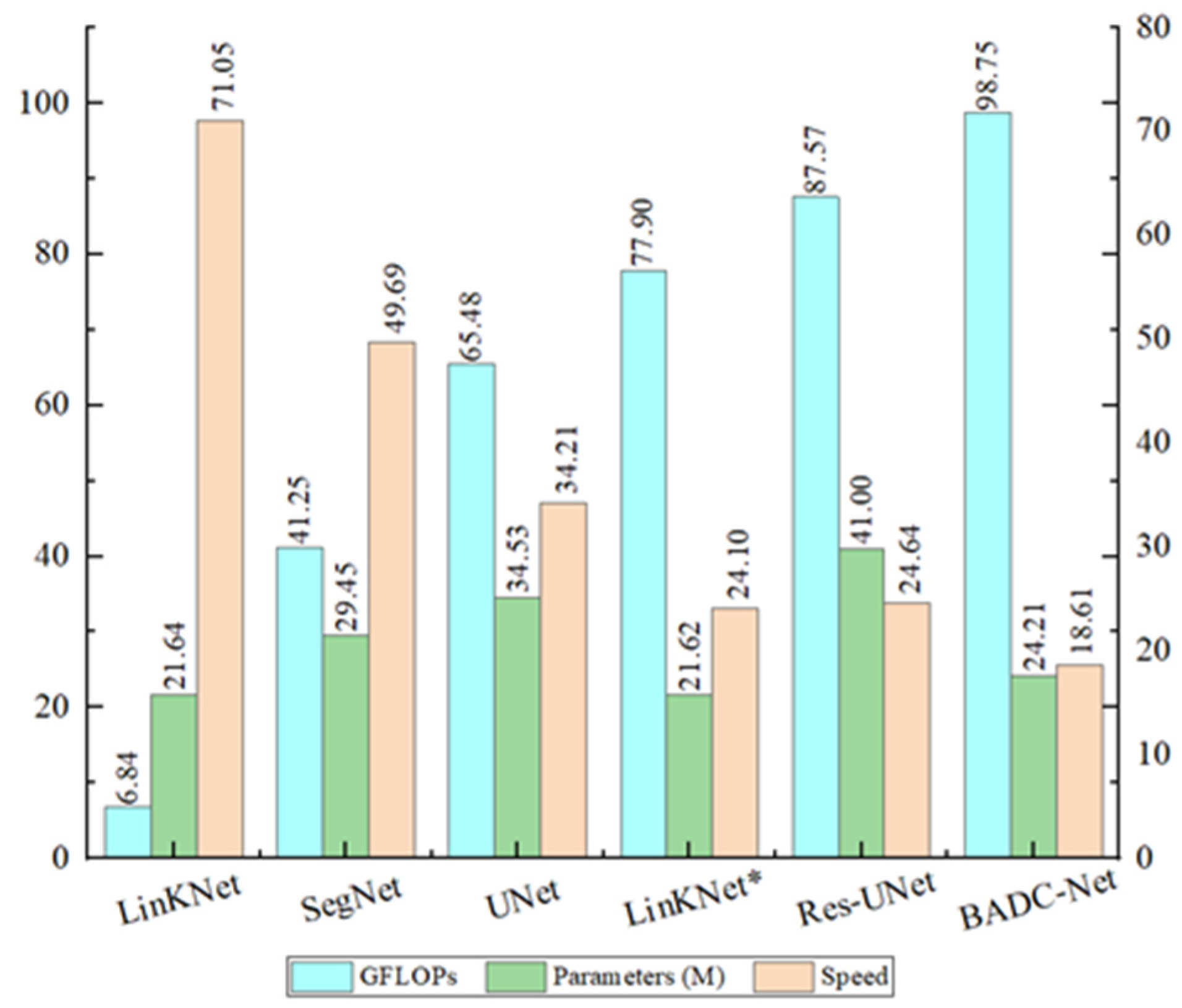
Figure 17.
Comparison of GFLOPs and parameters for different methods. GFLOPs and parameters are computed from a tensor of dimension 1 × 3 × 256 × 256. The speed is tested with a batch size of 2, full precision (fp32), input resolution of 3 × 256 × 256, and measured in examples/second.
Figure 17.
Comparison of GFLOPs and parameters for different methods. GFLOPs and parameters are computed from a tensor of dimension 1 × 3 × 256 × 256. The speed is tested with a batch size of 2, full precision (fp32), input resolution of 3 × 256 × 256, and measured in examples/second.
Table 1.
The encoder structure and the dimension variation of low level features. SA_1, SA_2, SA_3, and SA_4 denote the SA units of stages 1, 2, 3, and 4, respectively. Here, 3 × 256 × 256 represents the number of channels, height, and width, respectively. In addition, 3× Res-Block denotes three Res-Blocks.
| Stage | Template | Size |
|---|
| Input | - | 3 × 256 × 256 |
| 1 | 1 × 1 Conv + BN + ReLU | 64 × 256 × 256 |
| 3 × Res-Block |
| SA_1 |
| 2 | 4 × Res-Block | 128 × 128 × 128 |
| SA_2 |
| 3 | 6 × Res-Block | 256 × 64 × 64 |
| SA_3 |
| 4 | 3 × Res-Block | 512 × 32 × 32 |
| SA_4 |
Table 2.
Experimental environment and parameter settings.
Table 2.
Experimental environment and parameter settings.
| Hardware Configuration | Parameter Settings |
|---|
| Operating system | CentOS 7 | Epoch | 100 |
| DL framework | Pytorch 1.7 | Batch size | 16 |
| Language | Python 3.7 | Optimizer | Adam |
| GPU | 24G | Initial learning rate | 1 × 10⁻⁴ |
Table 3.
Accuracy evaluation results of different methods on the WHU building dataset. PISANet and Chen’s model are implemented by [
56] and [
4] respectively. ‘-’ denotes that the paper did not provide relevant data.
Table 3.
Accuracy evaluation results of different methods on the WHU building dataset. PISANet and Chen’s model are implemented by [
56] and [
4] respectively. ‘-’ denotes that the paper did not provide relevant data.
| Methods | OA (%) | P (%) | R (%) | F1 (%) | IOU (%) |
|---|
| U-Net | 98.54 | 93.42 | 92.71 | 93.06 | 87.02 |
| Res-UNet | 98.49 | 91.44 | 94.00 | 92.70 | 86.40 |
| LinkNet | 97.99 | 92.16 | 89.09 | 90.60 | 82.82 |
| LinkNet* | 98.72 | 94.88 | 93.02 | 93.94 | 88.57 |
| SegNet | 97.15 | 85.90 | 86.78 | 86.33 | 75.95 |
| DeeplabV3 | 97.82 | 88.93 | 90.16 | 89.54 | 81.06 |
| PISANet | 96.15 | 94.20 | 92.94 | 93.55 | 87.97 |
| Chen’s | - | 93.25 | 95.56 | 94.40 | 89.39 |
| B-FGC-Net | 98.90 | 95.03 | 94.49 | 94.76 | 90.04 |
Table 4.
Accuracy evaluation results of different methods on the INRIA aerial image labeling dataset. AMUNet and He’s model are implemented by [
32] and [
3] respectively. Here, ‘-’ denotes the unknown results that were not given by the authors.
Table 4.
Accuracy evaluation results of different methods on the INRIA aerial image labeling dataset. AMUNet and He’s model are implemented by [
32] and [
3] respectively. Here, ‘-’ denotes the unknown results that were not given by the authors.
| Model | OA (%) | P (%) | R (%) | F1 (%) | IOU (%) |
|---|
| U-Net | 96.10 | 84.76 | 87.76 | 86.24 | 75.80 |
| Res-UNet | 95.95 | 83.94 | 87.49 | 85.68 | 74.95 |
| LinkNet | 95.48 | 83.61 | 84.82 | 84.21 | 72.73 |
| LinkNet* | 96.55 | 86.85 | 88.93 | 87.88 | 78.38 |
| SegNet | 95.46 | 80.72 | 86.89 | 83.69 | 71.96 |
| DeepLabV3 | 95.80 | 84.58 | 86.04 | 85.30 | 74.37 |
| AMUNet | 96.73 | - | - | - | 76.96 |
| He’s | - | 83.50 | 91.10 | 87.10 | 77.20 |
| B-FGC-Net | 96.70 | 87.82 | 89.12 | 88.46 | 79.31 |
Table 5.
Evaluation results of different levels of SA units on the WHU building dataset. Note: the No. 1 model has no SA unit, and the No. 5 model is the B-FGC-Net.
Table 5.
Evaluation results of different levels of SA units on the WHU building dataset. Note: the No. 1 model has no SA unit, and the No. 5 model is the B-FGC-Net.
| No. | SA_4 | SA_3 | SA_2 | SA_1 | F1 (%) | IOU (%) |
|---|
| 1 | | | | | 94.38 | 89.30 |
| 2 | ✓ | | | | 94.52 | 89.62 |
| 3 | ✓ | ✓ | | | 94.54 | 89.65 |
| 4 | ✓ | ✓ | ✓ | | 94.58 | 89.72 |
| 5 | ✓ | ✓ | ✓ | ✓ | 94.76 | 90.04 |
Table 6.
Evaluation results of different global feature information awareness schemes on the WHU Building Dataset. Note: GFLOPs and parameters are computed from a tensor with a size of 1 × 512 × 32 × 32. The speed is tested with a batch size of 2, full precision (fp32), input resolution of 3 × 256 × 256, and measured in examples/second.
| No. | Methods | GFLOPs | Parameters (M) | Speed | F1 (%) | IOU (%) |
|---|
| 1 | PPM | 0.5417 | 0.7895 | 18.90 | 94.32 | 89.24 |
| 2 | ASPP | 4.0969 | 4.1318 | 17.19 | 94.39 | 89.37 |
| 3 | DCU | 12.082 | 11.799 | 16.93 | 94.60 | 89.75 |
| 4 | GFIA | 0.3036 | 0.2939 | 18.61 | 94.76 | 90.04 |
Table 7.
Ablation study with different component combinations on the WHU Building Dataset.
Table 7.
Ablation study with different component combinations on the WHU Building Dataset.
| No. | Baseline | SA | GFIA | CLFR | F1 (%) | IOU (%) |
|---|
| 1 | ✓ | | | | 94.02 | 88.71 |
| 2 | ✓ | ✓ | | | 94.44 | 89.46 |
| 3 | ✓ | ✓ | ✓ | | 94.56 | 89.68 |
| 4 | ✓ | ✓ | ✓ | ✓ | 94.76 | 90.04 |
