1. Introduction
Over the years, dense stereo matching has been studied persistently in the field of computer vision, remote sensing, and photogrammetry, as the corresponding applications keep promoting the development of self-driving, urban digitization, topographic survey, forest management, etc. [
1,
2,
3,
4]. Given a pair of images with the camera parameters and the relative distance (baseline) in between, the object depth is computed which extends 2D image information to 3D knowledge of the scene [
5]. In stereo matching, the depth is obtained in the form of disparity which presents the (horizontal) displacement of two corresponding pixels from each of the (rectified) stereo pair, respectively. A disparity map allows each pixel to be triangulated to its location in the 3D space. Stereo vision methods define two terms for locating correspondences, the data term and smoothness term. The former searches pixels with similar intensity as potential matches, while the latter requires close disparity predictions between neighboring points for spatial smoothness. Semi-Global Matching (SGM) is a representative method in stereo matching [
6]. The algorithm acquires dense correspondences via a simple pixel-wise cost comparison under a disparity searching range, and guarantees the (piece-wise) smoothness of the reconstructed surface simultaneously. For each target pixel, the previous point along a certain path is also considered to avoid neighboring disparity inconsistency. By repeatedly applying the strategy through multiple (normally 8 or 16) symmetric paths, 2D regularization is performed while keeping the algorithm computationally feasible.
As more high-quality, high-resolution data become available, the computational cost of dense matching rises exponentially, especially in the field of remote sensing. To limit the memory usage and runtime, Rothermel [
7] proposed tSGM. Images are firstly downsampled to several scales constituting a pyramid structure, in which the dense matching is applied from the lowest resolution to the highest, level by level. On the pyramid top, the disparity range is downscaled accordingly together with the image size, leading to reduced workload. The matching result is then passed to the next higher resolution level as an initial prediction, from which a small disparity buffer is set as a new search range to locally refine the estimation. The coarse-to-fine scheme thus greatly reduces the demand for memory and runtime. Moreover, the influence of ambiguous disparity candidates is limited. Additionally, this strategy enables the use of deep learning-based algorithms, which typically only support small search ranges due to memory limits on datasets with large disparity ranges of sometime several thousand pixels, as typically occurring in extreme mountainous regions, such as the Himalayas.
Recently, Zhang et al. [
8] introduced their GA-Net, which approximates SGM as a differentiable Semi-Global Guided Aggregation (SGA) layer, to construct an end-to-end neural network for stereo matching. All the user-defined parameters in SGM can be learned; thus, the smoothness requirement is satisfied in a smarter way depending on the specific scene situation. With SGA and only a few 3D convolutional layers to regularize the cost volume, GA-Net is more efficient than other networks, e.g., GC-Net [
9], PSMNet [
10], etc., and achieves state-of-the-art performance. For processing high-resolution remote sensing data, however, the training and prediction are still memory- and time-consuming (days are needed for training on patches of 384 × 576, with [0, 192] as the disparity search range, consuming around 15 GB GPU memory for each batch).
Inspired by tSGM and some corresponding pyramid networks [
11,
12,
13], we adjust GA-Net to a pyramid architecture, and propose our GA-Net-Pyramid. The disparity is initially estimated for the full depth range at the coarsest resolution, then refined through the pyramid. Thus, we enhance the efficiency of the algorithm significantly, with moderately decreased accuracy especially for remote sensing data. To summarize our contributions:
The rest of the paper is organized as follows: In
Section 2, traditional stereo methods, SGM and its variants are recapped, which enlighten the main idea of GA-Net and our GA-Net-Pyramid. We also describe representative learning-based algorithms, from hybrid approaches replacing certain traditional components with deep learning-based ones, to full end-to-end stereo networks. Afterwards, we state the principle of our method, GA-Net-Pyramid, with a review of its prototype GA-Net in
Section 3. In
Section 4, we present a detailed comparison between GA-Net and our GA-Net-Pyramid on various datasets. At last, we discuss the strengths and limitations of the method in
Section 5, and conclude the paper in
Section 6.
2. Related Work
2.1. Traditional Stereo Methods
Conventional stereo matching algorithms define two terms to find dense correspondences from a stereo pair, data term and smoothness term [
5]. The data term measures the photo consistency between potentially matched pixels through a pre-defined disparity range. The smoothness term guarantees a smooth reconstructed surface by limiting neighboring points’ disparity differences. SGM well balanced the two terms via a scanline optimization strategy, which was widely applied thanks to the good compromise between accuracy and efficiency [
6,
18,
19]. The strategy was further improved with a dynamic searching range for correspondences through a pyramid structure, leading to tSGM which consumed less memory and runtime [
7]. As More Global Matching (MGM) was proposed, the support from neighboring pixels was increased without extra overhead, by additionally considering the previous scanline visited already [
19,
20]. Compared with other traditional stereo methods [
21,
22,
23,
24,
25], which may solely rely on the cost function and winner-takes-all (WTA) strategy resulting in limited accuracy, or struggle to find the minimum global energy under certain runtime or memory budget, the SGM variants achieve robust stereo estimation consuming reasonable computational resource.
2.2. Learning-Assisted Stereo Methods
2.2.1. Integration of Conventional Stereo Methods and Machine Learning
Recent advances in machine/deep learning and convolutional neural networks (CNNs) enable the learning of data representation [
26], and promote the development of stereo matching with a series of state-of-the-art algorithms. Deep learning could be exploited to extract features from images, in order to better measure the similarity for matching cost calculation. Zbontar and LeCun [
27] used a Siamese network [
28] to extract features from two patches symmetrically, after which a cost volume was constructed and regularized by SGM. The idea was adjusted by Luo et al. [
29] based on multi-class classification, achieving faster estimation. Regarding the cost aggregation and disparity computation, Seki and Pollefeys [
30] proposed their SGM-Net to learn the penalty terms for conflicting disparity predictions from neighboring points. Michael et al. [
31] considered a specific weight for each scanline in SGM to achieve a weighted 2D scanline optimization, since varying performance could be obtained via each scanline depending on the scene structure. Poggi and Mattoccia [
32] constructed a feature vector for each pixel according to the disparity estimation via a single scanline. The feature represented the statistical dispersion of surrounding disparities, which could be analyzed by a random forest to predict a confidence measure of the scanline for a weighted scanline summation. Similar work was accomplished in [
33,
34]. The disparity predicted by each scanline and the corresponding costs were fed to a random forest, so that the better performed scanlines were adaptively selected. The corresponding disparity estimation could serve as a reference to guide the further stereo prediction.
2.2.2. End-to-End Stereo Networks
The above methods mainly integrated deep learning with traditional stereo matching techniques for better performance, which were then followed by encoder-decoder structures for depth prediction as an end-to-end system. Dosovitskiy et al. [
35] firstly presented a network, FlowNet, to estimate optical flow directly from a stereo pair. They used a correlation layer to measure the similarity between corresponding patches. Mayer et al. [
15] then designed a large synthetic dataset, Scene Flow, allowing an initial training of deep neural networks before adjusting to specific scenarios. They also proposed DispNet and DispNetCorr, as one of the first end-to-end stereo matching networks. Kendall et al. [
9] proposed GC-Net, which applied 3D convolutions to regularize the cost volume, with both geometry and context information incorporated. Chang and Chen [
10] introduced a pyramid pooling module in their PSMNet to aggregate multi-scale features. Thus, the global context and local details were simultaneously contained within the cost volume. Guo et al. [
36] improved PSMNet by proposing the group-wise correlation stereo network (GwcNet). They constructed a group-wise correlation-based cost volume which required less parameters for the cost aggregation, achieving similar performance as PSMNet. Zhu et al. [
37] proposed a multi-scale pyramid aggregation module to handle the cost volume, leading to MPANet with significantly better disparity estimation for foreground objects. Xu and Zhang [
38] proposed AAnet, utilizing intra- and cross-scale cost aggregation, which delivered better results for depth discontinuities and large textureless area. Wang et al. [
39] applied a recurrent unit to iteratively refine the stereo estimation, and designed a pyramid voting module to produce a semi-dense disparity map for self-supervision. Confident disparity prediction was achieved via seeking consistent estimation across scales. Inspired by SGM, Zhang et al. [
8] proposed the GA-Net using so-called SGA layer for cost aggregation, to replace 3D convolution which was computationally expensive. They achieved great performance on multiple benchmark datasets, which coincided with the idea from [
40] that classical stereo matching methods could serve as a robust guideline to develop deep learning-based algorithms, rather than designing a pure learning architecture. Semantic information could also be involved for stereo matching problems [
41,
42] as the object boundaries mostly corresponded to the depth discontinuities. The two tasks supported each other leading to a win-win situation. Other works included cost distribution study, disparity refinement, cross-domain prediction, stereo neural architecture search, etc., which boosted the state-of-the-art constantly [
40,
43,
44,
45,
46,
47].
Recently, the pyramid architecture was tested in a learning-based stereo framework, since the efficiency could be largely enhanced via a coarse-to-fine estimation [
11,
12,
13,
48,
49]. Regarding the architecture in [
11,
12,
13] as a baseline model, the stereo correspondences were firstly located on the pyramid top using downsampled features. Then, the disparity was iteratively refined through the network towards the pyramid bottom in full resolution, which considerably reduced the computational effort and GPU memory consumption. Chang et al. [
48] benefited from the architecture to achieve real-time performance, with an attention-aware feature aggregation module for better representative ability of the feature. Compared with these methods, our contributions are different. At first, we additionally test our model on airborne and spaceborne images. We fill the application gap of the previous research, considering the very limited test cases applying newly proposed computer vision algorithms in the field of remote sensing. The proposed model is proven effective to process stereo imagery with large disparity range (thousand pixels) over mountain areas. It should be noted that our model acquires no supervision in training phase on stereo data with large baselines, with no need to normalize/denormalize the disparity measurement in test phase as [
50]. This is, to the best of our knowledge, a novel showcase of adapting well-performed computer vision models to deliver high-quality geographical products in extreme regions. In addition, our baseline is the up-to-date model GA-Net-deep from [
8], rather than the shallower and less accurate version GA-Net-11 used in [
49].
3. Methodology
In this section, we recap GA-Net by presenting the proposed SGA and LGA (Local Guided Aggregation) layers, which approximate SGM for cost regularization and protect thin structures, respectively. SGM applies the scanline optimization strategy to efficiently locate stereo correspondences and avoids the streaking problem. For a detailed description of SGM, we encourage readers to follow the papers [
6,
51]. Afterwards, we describe our pyramidal extension of GA-Net, GA-Net-Pyramid. Two architectures are proposed. The first model explicitly downsamples the input stereo pair according to the pyramid level, and simply applies GA-Net on each level to regress disparity. The second model applies a different feature extraction strategy via a U-Net [
52] structure to generate multi-scale features implicitly.
3.1. GA-Net
In traditional SGM, the scanline optimization technique [
53] is applied to satisfy the spatial smoothness, by limiting the depth difference between neighboring pixels. To avoid the streaking problem, a pixel is accessed through multiple scanlines simultaneously along several canonical directions, typically 8 or 16, to consider the disparity estimation from its neighbor. Along a certain scanline traversing in direction
r, the cost for a pixel located at the image position
p assuming
d as the disparity, is calculated as:
In the above equation, the photo inconsistency is measured by , while and are defined for penalizing the prediction when the previous neighboring point p − r prefers a different disparity value. In practice, however, two problems exist. Firstly, the users need expertise to determine appropriate and to punish neighboring disparity inconsistency. Tuning of and additionally depends on scene structure and the used similarity measure. Moreover, the values of and are fixed throughout the stereo processing or simply adapted according to, e.g., pixel gradients, which are not optimal for all the pixels within the image, especially under a varied scene structure, e.g., from plains to mountains.
GA-Net addresses these issues by introducing the SGA layer, a differentiable approximation of Equation (
1) that is suitable for an end-to-end trainable network. Specifically, the master epipolar image provides guiding information through a sub-network to better penalize depth discontinuity, and enable a self-adaptive parameter setting. Thus, the penalty terms for conflicting neighboring disparities are determined according to the pixel location and scanline direction, which is more reasonable for smoothness regularization. Via the guidance sub-network, a weight is supplied for each term in Equation (
1) to simulate the scanline optimization in SGM, leading to the following equation:
Compared with Equation (
1), the punishment from
and
is replaced by the relative importance (weight)
of each term, which is predicted separately for each pixel along a directed scanline. Moreover, there are two differences with SGM, one of which is that the first/external minimum operation is substituted by a weighted sum. This can be regarded as a replacement from a max-pooling layer to a convolution with strides, which is proven effective without accuracy loss [
54]. In addition, the second/internal minimum search is changed to a maximum, which embodies the learning target to maximize the probability at the ground truth disparity rather than minimizing the cost. To avoid the exploding accumulation of
along the scanline,
is also included within the weighted summation, with the sum of all the weights equal to 1. Thus, SGA is finally formulated as:
In SGM, the cost
from each scanline is simply summed up to approximate 2D smoothness, which was demonstrated to be not reasonable for incurring inferior scanlines [
33,
34]. Accordingly, GA-Net takes the maximum as
to keep the best information.
The guidance sub-network also provides weights for another layer, LGA, to further filter the cost volume as below:
from which a 3D neighborhood (in both spatial and disparity dimensions) centered around each pixel within the cost volume is utilized for a weighted average to protect thin structures. Afterwards as suggested by [
9], a softmax operation
is applied to the filtered cost volume in order to acquire a normalized probability for each disparity candidate (from [0,
]) and regress the final disparity value
as:
3.2. GA-Net-Pyramid with Explicit Downsampling
GA-Net adapts the scanline optimization scheme to an end-to-end stereo matching system. Inspired by SGM, the disparity of each pixel can be estimated with the support from all the previous neighbors along multiple paths, instead of a pure convolution-based encoder-decoder to regularize the cost volume. Furthermore, the proposed SGA and LGA layers are computationally more efficient than 3D convolutions, which are used by most state-of-the-art methods [
9,
10]. However it can still take days to train a well performing model, when the computational power is limited. In our case, for example, the training on the Scene Flow dataset (patch size 384 × 576), which is normally used by most stereo matching networks for the initial learning phase, takes around 12 days to finish 8 epochs on two Quadro P6000 GPU cards. Hence, the employment of the network is hampered. In the field of remote sensing, it can be imagined that GA-Net would struggle to process high-resolution aerial or satellite stereo data, especially for wide baseline stereo pairs requiring larger disparity search ranges.
Rothermel [
7] proposed an improved SGM, tSGM, which constructed a pyramid architecture to search correspondences between the stereo pair from coarse to fine. Based on this strategy, comparable quality was achieved with far less memory and runtime consumed. This inspires us to restructure GA-Net with a pyramid architecture as well, to regress the depth from coarse to fine.
Figure 1 presents the schematic overview of our GA-Net-Pyramid. Three pyramid levels are depicted which could be extended. We use the same stacked hourglass module (a double U-Net structure) as GA-Net, which is essentially a Siamese network [
28] for symmetric feature extraction from the left and right image, respectively. The input of the feature extraction module, however, is a stereo pair downsampled in accordance with the pyramid level. Afterwards, the cost volume is generated and then processed by SGA and LGA for disparity regression, in order to guide the subsequent level for the disparity refinement until the original resolution is recovered.
3.2.1. Pyramid Top
We start from the pyramid top with the original image downscaled by a factor of 4 along both row and column directions in our implementation (termed as ‘Scale 1/4’ in
Figure 1). Then, the feature is extracted to construct a 4D cost volume by concatenating the left and right feature maps along the channel dimension, with a horizontal shift indicated by a disparity candidate within the search range. Assuming the cost volume on the original full-resolution image is of size
, for the image height, width, the maximum disparity, and twice the channel number of the generated feature maps, respectively, our cost volume on the pyramid top reaches a highly reduced dimension as
. Thus, the memory consumption and computational complexity are decreased by a factor of 1/64.
Afterwards, the cost volume enters the cost aggregation block containing SGA and LGA layers, for which the guiding information is obtained from the downscaled master epipolar image. At last, the filtered cost is used for the following disparity regression as GA-Net. Thus, a disparity map of the downsampled image ‘Scale 1/4’ is obtained for the pyramid top. From here, the depth of the scene is already roughly estimated and the large-scale context is perceived, which provides a good guidance for the following processing.
3.2.2. The Other Pyramid Levels
Based on the prediction of the pyramid top, the other levels thus only need to locally refine the disparity values. Therefore, the disparity map from ‘Scale 1/4’ level is upsampled by a factor of 2 via bilinear interpolation, to match the resolution of ‘Scale 1/2’ level as an initial estimation
. Feature maps are computed for the left and right image of ‘Scale 1/2’ level as
and
, respectively. Assuming
is accurate enough, we can warp
according to
which would perfectly match
. However, considering the details lost through downsampling on the pyramid top and the corresponding matching error, a small shift would exist between the left and the warped right feature, which is named disparity residual and should be additionally considered for a perfect match. Accordingly, a cost volume
is built in size of
for ‘Scale 1/2’ level. Here,
is a pre-defined threshold, leading to a range [
] around the initial disparity estimation
for refinement. The cost volume is thus formed by concatenation of
and
as:
In Equation (
6),
x and
y are the indices of a pixel along the width and height dimension. ⊕ represents the concatenation. Then, the cost volume is regularized by SGA and LGA, and a residual disparity map
is calculated via multiplying each residual candidate to the corresponding probability and summing them up. The disparity estimation for the current level is obtained by adding the residual and the previously upscaled disparity map as:
.
The stereo pair on ‘Scale 1/2’ level is twice larger in height and width; however, the search for correspondences is restricted within a narrow range. Hence, only a small overhead is accumulated. We apply the same procedure for the remaining pyramid level, to continuously improve the disparity estimation until the original resolution is reached.
Each pyramid level only requires the input epipolar imagery at its level and the disparity image of the previous level. For an efficient and memory saving implementation during disparity estimation, computation of the levels could be decoupled to significantly lower the memory footprint while allowing large input image sizes. Compared to GA-Net, it is thus feasible to significantly increase both image size and disparity range, as only the pyramid top needs to process the full disparity search range, for example, processing of images with a four times larger width, height, and disparity range is possible without additional GPU memory requirements in this case. Note that the evaluation in
Section 4 is recorded without adding these optimizations.
3.2.3. Loss
We train the model using the same smooth
loss function as GA-Net in [
8]. However, our pyramid architecture predicts more than one disparity map, which should all be considered to allow for intermediate supervision. Hence, a weight is assigned to each pyramid level for a weighted loss summation as:
in which
denotes the disparity predicted by the pyramid level
i (starting from 1 at the pyramid top), and
is the corresponding ground truth.
l computes the smooth
loss from the disparity difference. A weight
is assigned to the level
i for a weighted summation through all
N pyramid levels. The disparity map from each level is upscaled to the original full resolution before computing the loss. As the estimation is improved from the pyramid top to the bottom, the corresponding weight is also increased (details for parameter setting are in
Section 4).
3.3. GA-Net-Pyramid with Implicit Downsampling
The paper focuses on presenting a more efficient model based on the structure of GA-Net, in order to achieve robust estimation on datasets from multiple domains. Thus, we design different feature extractors and observe the corresponding performance, so that an appropriate model could be used to handle specific data types. The architecture in
Figure 1 simply applies GA-Net in a pyramidal manner, which takes the linearly downsampled stereo pair as input to extract features for further processing. Therefore, we propose another architecture to implicitly learn the downsampled feature, as displayed
Figure 2, such that both explicit and implicit image downsampling strategies are tested.
Instead of downsampling the input stereo pair level by level, we only use the stacked hourglass once to extract the feature from the original (full-resolution) images for feeding all the pyramid levels. The input images are firstly downsampled via convolutions with stride two, and then deconvolved to gradually recover the resolution, in which a skip connection is exerted between corresponding feature maps of the encoder and decoder at the same resolution. Before reaching the original size, we directly extract the intermediate feature maps from the decoder to feed each level, as long as the expected resolution is acquired. To differentiate the GA-Net-Pyramid with explicit and implicit downsampling, in the following sections we name the two variants as GA-Net-PyramidED and GA-Net-PyramidID, respectively.
As the disparity is estimated and refined through the pyramid, we add a Spatial Propagation Network (SPN) as a post-processing step to explore its influence on the matching results. SPN is capable of sharpening the object boundaries, by learning from the source image (in our case, the master epipolar image) in a data-driven mode, which is appropriate as a further refinement in our pyramid architecture, especially for close-range data with rich details. Hence, four models are finally proposed including GA-Net-PyramidED and GA-Net-PyramidID, respectively, with or without SPN added at the end of the pyramid bottom.
4. Experiments
In this section, we compare our GA-Net-Pyramid with GA-Net through a series of experiments on close-range, including Scene Flow and KITTI-2012, aerial, and satellite stereo datasets. For a fair comparison, the implementation details are rigidly controlled between the two algorithms. Regarding the training, we use the same patch size with a pre-defined disparity search range, to train the networks for certain epochs, based on Adam optimization strategy [
55]. Each stereo pair is normalized, according to the mean and standard deviation of the pixel values from each channel, before feeding to the network. SGA is applied along four directions (horizontally and vertically) for both GA-Net-Pyramid and GA-Net.
For GA-Net-Pyramid specifically, the number of pyramid levels is 3 and the search range for the disparity residual after the pyramid top is set as [−6, +6] to refine the matching results. Details about the pyramid setting are discussed in
Section 4.2.3. We apply 3 SGA and 2 LGA layers to regularize the cost volume on our pyramid top, which is the same as GA-Net. With regard to the other pyramid levels, only 1 SGA layer (with 2 LGA layers) is utilized due to the small disparity search range. The weight is set as 0.25, 0.5, and 1, to the pyramid level 1 (top), 2 and 3 (bottom), respectively, to calculate the final loss in Equation (
7). The implementation of the methods is based on Python and Pytorch.
4.1. Experiments on Close-Range Stereo Data
We firstly test the networks on Scene Flow and KITTI-2012 datasets, in which the scene structure is relatively complicated with rich details. Referring to most learning-based dense matching algorithms, we train the models on Scene Flow data from scratch, and utilize real data, KITTI-2012 in our case, for finetuning. Both the pre-trained and finetuned models are tested on the corresponding dataset. Regarding the former, the whole Scene Flow training dataset is used for training (8 epochs), while only 1000 stereo pairs from its validation set are selected for test to save time. On the other hand, 170 images from KITTI-2012’s training data are exploited to finetune the models for 800 epochs, with the remaining 24 images for test. All the data selection is random, so that a fair evaluation is achieved. In training, we use the same patch size (384 × 576) with the maximum disparity set to 192. The networks are trained with a batch size of two on two Quadro P6000 GPU cards.
4.1.1. Close-Range Stereo Data
Scene Flow is a synthetic dataset via randomly combining human-made objects with backgrounds from real images, which is used by most stereo networks for initial training. Afterwards, only a small dataset from a specific field is sufficient to adjust the model into practical scenarios. The dataset contains three subsets, namely FlyingThings3D, Monkaa and Driving, including around 35,000 images for training and 4370 images for validation. KITTI-2012 is a stereo dataset with a focus on outdoor street views, which is normally applied in the field of autonomous driving. The dataset includes 194 training and 195 test stereo pairs, with ground truth disparity maps based on LiDAR measurements provided or withheld.
4.1.2. Visualization and Evaluation on Close-Range Stereo Data
The pre-trained networks are firstly tested on the Scene Flow dataset. The quantitative and visual comparison between our pyramid models and GA-Net is shown in
Table 1 and
Figure 3. As indicated by the table, we calculate the percentage of pixels, for which the estimation error is smaller than 1, 2, and 3 pixels, respectively, and the end point error (EPE) for accuracy evaluation. Regarding the efficiency, the runtime and GPU memory consumption are reported. For all the experiments in this paper, the runtime in the test period is counted for processing the whole test dataset. Specifically, we generate a binary file to save the disparity value of each correspondence, and a png (Portable Network Graphics) file to visualize the result. In the tables, M denotes megabytes for the GPU memory consumed by each network, while the time spent in training and test is expressed in hours (h) or seconds (s). Better performance is highlighted in bold.
From the results, it is found that GA-Net outperforms the two pyramid models in accuracy; however, the latter consume much less memory and runtime in both training and test periods. In case of the close-range data, the objects are captured under an ideal viewing condition, thus very high resolution is achieved with plenty of details and texture information contained. Moreover, as Scene Flow is a synthetic dataset, the random arrangement of man-made objects makes the scene non-natural, non-logical, and highly complicated with many occlusions. Hence, our GA-Net-Pyramid is surpassed by GA-Net, considering the information loss due to a sequence of downsampling-upsampling through the pyramid levels. On the other hand, our hierarchical strategy highly simplifies the problem complexity, consuming far less computational source but at a much higher speed. Between the two pyramid models, GA-Net-PyramidED and GA-Net-PyramidID, similar accuracy is obtained. Regarding the SPN processing, a positive effect is achieved for both pyramid structures, while GA-Net-PyramidID could be improved by a larger extent. The experiments of this paper are implemented on a server open to multiple users; therefore, the runtime of each model could be slightly influenced by unknown processes. We recommend referring to the training time to evaluate the speed of the algorithms, especially for each pyramid model with similar efficiency, considering the relatively long training process compared with the test period. GA-Net-PyramidID is faster than GA-Net-PyramidED, since the feature extraction in the former case is applied only once on the full-resolution stereo pair, rather than repeatedly learning from the corresponding downsampled images level by level. In case of the GPU memory consumption, GA-Net-PyramidED performs better.
As for the figures in the paper, only the best performed pyramid model is visually compared with GA-Net, e.g., GA-Net-PyramidID+SPN on Scene Flow dataset. Accordingly, we display the master epipolar image, where the guidance information is acquired for SGA and LGA, the ground truth, and the corresponding results from each algorithm. The color bar at the end shows the disparity and error changes. In
Figure 3, it is found that GA-Net obtains a generally better disparity result than GA-Net-PyramidID+SPN, with clear edges and more details included. However, our pyramid model still produces a disparity map in good quality, even including superior depth results in certain regions. We discover that GA-Net-PyramidID+SPN is capable of better reconstructing hollow-shaped objects, e.g., the barrel and the shelf as indicated by the red arrows. The finding is also supported by the following experiments on the KITTI dataset.
The pre-trained networks are finetuned on part of KITTI-2012’s training data and tested on the remaining stereo pairs. In
Table 2 and
Figure 4, the corresponding quantitative and qualitative results are provided. Regarding the training efficiency, only the time spent for finetuning is recorded. Similar to the previous experiment, GA-Net acquires the best accuracy, however, the pyramid models are faster and more memory friendly. SPN still improves the results of all the pyramid models, among which GA-Net-PyramidID+SPN achieves the highest accuracy. It should be noted that our GA-Net-Pyramid performs better for real data, leading to a further reduced accuracy gap compared with GA-Net. From the visual inspection, the depth result of each algorithm is barely distinguishable. Moreover as mentioned before, we obtain a better depth prediction for hollow-shaped structures (see the regions indicated by the red arrows). KITTI-2012 does not provide ground truth for the whole scene; nevertheless, according to the image content, it is obvious that our pyramid architecture gives a clean and more reasonable depth estimation.
4.2. Experiments on Aerial Stereo Data
In this section, the networks are tested using our aerial data. The airborne and satellite (discussed in the following section) stereo processing is the target domain of this research, since the corresponding data are usually large in size and own a much wider stereo baseline, which presents a higher demand on the algorithm’s efficiency. The networks are trained on synthetic remote sensing data (854 stereo pairs) from scratch for 200 epochs, then finetuned on a subset (200 stereo pairs) of our aerial data for 100 epochs (data details are in
Section 4.2.1). We randomly select another 20 aerial stereo pairs, possessing no overlap with the finetuning data, to test the trained models. Image patches in size of 384 × 576 are randomly cropped for training, and the test images are 1152 × 1152. The data may contain negative or very large disparity values; hence, we exclude the stereo pairs with large baselines in order to keep the disparity range processible by both GA-Net-Pyramid and GA-Net. Accordingly, the disparity range is also set as [0, 192]. The models are trained with a batch size of two on two Quadro P6000 GPU cards.
In addition, SGM is utilized as a baseline model in our aerial and satellite experiments, since the algorithm is widely used in the field of remote sensing for dense reconstruction. We exploit Census [
56] to calculate the matching cost with a 7 × 7 window. The penalty terms
and
(see Equation (
1)) are set to 19 and 33, respectively. The cost from 8 symmetric scanlines along horizontal, vertical, and diagonal directions are accumulated to compute the disparity based on the WTA strategy, which is then further refined using a left-right consistency check.
4.2.1. Aerial Stereo Data
Nowadays, most state-of-the-art dense matching algorithms are data-driven deep neural networks [
8,
9,
10,
12,
41,
42,
43]. The high performance usually originates from a thorough training, for which a synthetic dataset is preferred for an initial learning phase, to avoid time-consuming data collection and annotation. In the field of remote sensing, nevertheless, a well-annotated stereo dataset is scarce. For example, the aerial image matching benchmark [
57,
58] provides reference data using LiDAR measurement. However, each algorithm is finally evaluated by the median of the DSM estimation from all the evaluated approaches, due to the limited accuracy of the reference data. Therefore, we propose a synthetic dataset, which is designed specifically for airborne and satellite stereo tasks. The dataset focuses on urban regions via referring to six city models provided by the software CityEngine: Paris, Venice, New York, Philadelphia, and two small development scenes. The models were exported and processed in Blender to preserve the textures and relevant information. Afterwards, we used BlenderProc [
59] to render the dataset according to the geometry of the model which included RGB images and the corresponding disparity maps. Considering both aerial and satellite platforms, the simulated camera for rendering was located at 200 m and 500 km above the cities, respectively. A total of 854 stereo pairs in size of 1024 × 1024 pixels were generated, with the ground sampling distance (GSD) ranging from 5 cm to 50 cm.
Regarding our real aerial data, we use the 4K sensor system mounted on a helicopter for the data collection [
60]. Three off-the-shelf Canon EOS cameras (one 1D-C and two 1D-X) constitute the imaging unit. The data contain geo-referenced images with a size of 17.9 megapixels, acquired over Gilching in the southwest of Munich, Germany. Equipped with 50-mm lenses looking in varying view directions, a field of view (FOV) up to 104
is reached. The flight height was 500 m above ground, enabling 6.9-cm nadir GSD. A multi-view stereo matching based on SGM was applied, in which the calculated heights (depths) from multiple highly overlapped images were fused to achieve a high-quality digital surface model (DSM). The DSM was used to compute disparity maps for each stereo pair, which were utilized as reference data for finetuning and evaluation.
4.2.2. Visualization and Evaluation on Aerial Stereo Data
In
Table 3, the performance of each algorithm is recorded. We firstly find that all the GA-Net models outperform the baseline SGM by a certain margin. Moreover, our pyramidal revision leads to a very small accuracy decrease compared with the original structure, but highly improves the efficiency. Our GA-Net-PyramidED (without SPN added) is the best performing pyramid model, which is only around 1% worse than GA-Net in accuracy. Nevertheless, the pyramid models are about 8 and 7 times faster than GA-Net, by only expending around 25% and 40% memory usage for training and prediction, respectively. It should be noted that for airborne data, SPN cannot improve the performance for either of the pyramid models, which is different from the close-range experiments. A visual comparison among the methods is provided in
Figure 5.
We select two regions, one vegetation and one building area from the test data for the visualization. It is shown that GA-Net-PyramidED archives good performance in airborne stereo matching. When the scene is relatively simple, containing fewer depth discontinuities and a smooth depth change, the hierarchical estimation and refinement of disparity is capable of highly enhancing the efficiency, without a noteworthy sacrifice of the result’s quality.
4.2.3. Pyramid Setting
To further understand our GA-Net-Pyramid when applied in the field of remote sensing, we explore the impact of different pyramid architectures using our aerial data. Regarding the pyramid structure, two variants are the most important factors, the number of pyramid levels and the residual search range for disparity refinement. The main difference between GA-Net-PyramidED and GA-Net-PyramidID is the strategy to extract features, which is not directly related to the above two factors. In addition, our two pyramid models achieve similar accuracy. Therefore, we select GA-Net-PyramidED without SPN for post-processing to study the pyramid setting, since it is the more intuitive pyramidal modification of GA-Net. As for the number of pyramid levels, we start from 2, since a 1-level GA-Net-Pyramid will degenerate to GA-Net, to 4 levels, with a fixed residual range [−6, +6]. The model is trained on our synthetic dataset from scratch and evaluated on the same test data. We use the same hyperparameter setting as before, except that the size of the training patches changes to 384 × 768 to facilitate the downsampling when more levels are applied. We train the model on one GPU card due to the less memory requirement of GA-Net-Pyramid. The results are in
Table 4.
According to the table, it is found that the architecture with 4 pyramid levels acquires the best efficiency. However, with slightly increased memory and runtime, the model with 3 pyramid levels achieves better results. Along with GA-Net-PyramidED regresses towards GA-Net (from 3 to 2 levels), the efficiency drastically deteriorates as expected, nevertheless, without a noticeable improvement of the accuracy. Therefore, we determine to use the number of pyramid levels as 3. Then, we adjust the residual search range to [−3, +3], [−6, +6] and [−12, +12], respectively. The model is also trained from scratch on our synthetic dataset using one GPU card, and tested on the same 20 aerial images. We keep the training setting unchanged, except that the patch size is set back to 384 × 576. In
Table 5, the performance for different residual search ranges is recorded.
Table 5 indicates that as the residual range becomes larger, the efficiency naturally decreases. Moreover, when the residual buffer expands over [−6, +6], the accuracy cannot be further enhanced. Hence, the structure of our pyramid is determined as 3 levels, with the maximum/minimum residual set as 6/−6. To keep the experiments consistent, the pyramid structure is used for both GA-Net-PyramidED and GA-Net-PyramidID in this paper.
4.3. Experiments on Satellite Stereo Data
The flight campaign regarding our aerial 4K images was performed during a WorldView-3 stereo acquisition of the same area [
61]. Due to the minimal time difference of less than 1 hour of each aerial image from the satellite images, the higher resolution airborne data are well suited as reference data for the satellite stereo matching to finetune the models and evaluate the results. This is a notable improvement over other satellite stereo datasets [
17,
62], which do not provide sub-pixel disparity accuracy due to different sensing modalities and scene changes due to time difference between the image and ground truth acquisition. In contrast, the data used in this article allow reliable evaluation for 1- and 2-pixel accuracy metrics. This is especially import for photogrammetry and remote sensing, as many applications require highly precise elevation measurements.
Similar to
Section 4.2, the networks are pre-trained on our synthetic remote sensing data for 200 epochs, and finetuned on the generated satellite training data for 150 epochs. The training conditions stay the same, including the patch size (384 × 576), disparity range ([0, 192]), batch size (2), GPU usage (2 Quadro P6000 cards), etc. SGM is also tested for reference.
4.3.1. Satellite Stereo Data
WorldView-3 is a very-high-resolution imaging satellite currently offering the most detailed publicly available spaceborne imagery, at a resolution of 30 cm. After bundle-adjustment of the data with the 4K aerial imagery and DSM as reference, we generated an epipolar rectified stereo pair using the algorithm implemented by the CARS stereo pipeline [
63]. Similar to the aerial imagery, a reference disparity map was calculated by projecting each point of the 4K DSM into the epipolar satellite stereo pair. The stereo pair has a dimension of 20,815 × 28,264 pixels, which was cut into 98 tiles (in size of 1152 × 1152) owning an overlap larger than 25% with the 4K data coverage. From them, 78 tiles were randomly selected for finetuning the pre-trained GA-Net models, with the other 20 image pairs as the test data.
As the airborne data were geo-referenced in two separate blocks using differential GPS and only few ground control points (GCPs), a slight height offset was found between the aerial and satellite data, yielding disparity differences between the aerial reference and the satellite stereo pair in the pixel range, but rising up to 4 pixels at the corner of one aerial block. Since these systematic differences strongly affected training and evaluation of the networks, a second-order offset surface was fitted to the difference of the airborne reference disparity map and the satellite disparity map estimated by SGM, on each of the 98 tiles. The offset was added to the reference disparity map to alleviate the systematic bias which was reduced from 0.97 to 0.51 pixels.
4.3.2. Visualization and Evaluation on Satellite Stereo Data
In
Table 6, we record the performance of GA-Net-Pyramid, GA-Net and SGM. Similar to the results of airborne data, GA-Net achieves the highest accuracy, after which GA-Net-PyramidED still acquires the best performance among all the other models. The 1-pixel accuracy of our GA-Net-PyramidED, without SPN added for post-processing, is only surpassed by GA-Net by 0.08%. However, the former is around 8 and 13 times faster than the latter, consuming only 23% and 36% GPU memory in training and test, respectively. In addition, GA-Net-PyramidED performs better than GA-Net_PyrmaidID, with less GPU memory consumption but longer training time. SPN also impairs the performance of the pyramid models which is consistent with our experiments on aerial data. The visual comparison is in
Figure 6, including a vegetation and a building area as well. It is found that both networks predict a smoother disparity map than SGM, with less erroneous estimation. Moreover, similar results are obtained between our GA-Net-PyramidED and GA-Net, considering the reconstruction density and quality.
4.3.3. Stereo Processing over Mountain Area
In this section, we apply our pyramid network on a stereo pair with a large disparity range, in order to indicate the model’s ability to process large-scale remote sensing data. The imagery is from WorldView-2 [
64] at a resolution of 50 cm, covering the Matterhorn mountain, Switzerland. We select a stereo pair with 14
conversion angle for which the disparity varies in range of thousand pixels, due to the very large ground height difference from 1800 m to 4478 m. The best performing model finetuned in our previous satellite experiments, GA-Net-PyramidED, is directly used for disparity prediction in this test. Regarding the evaluation, we follow our processing chain in
Section 4.3.1, using an aerial dataset with good stereo geometry to the same area to generate reference data. The test region, the reference disparity map, and our stereo results are displayed in
Figure 7.
The mountain peak is located at the center of the image with a disparity up to around 1250 pixels; thus, we set the disparity range as [0, 1248]. Note that the model we use receives no supervision and knowledge regarding the mountain area with that large disparity difference. However, we achieve a 3-pixel accuracy of 87.34%. There are temporal inconsistencies between the satellite and reference data, leading to varying snow cover. Therefore, we use 3-pixel as the threshold. The visual comparison shows very similar results between our disparity prediction and the reference, considering the reconstruction density, smoothness, etc. Disparity holes are found from certain regions in our results. According to the image content, the regions are in shadow with limited texture information, where the network suffers from collecting enough information to locate the correspondences.
In the test period, the patch in size of 768 × 6912 is fed to the network for disparity prediction. Considering the disparity range [0, 1248], GA-Net will theoretically need more than 200 GB GPU memory to process the same data. Our GA-Net-PyramidED, however, consumes only around 20 GB.
5. Discussion
Based on a pyramid architecture, our GA-Net-Pyramid is able to roughly estimate the depth from a downsampled feature, and then refine the prediction level by level until the original resolution is recovered. Thus, the efficiency is significantly enhanced with the accuracy maintained to be comparable with GA-Net on remote sensing datasets. Some technical details are found below.
We firstly propose GA-Net-PyramidED which applies the GA-Net model hierarchically. In our experiments on airborne and satellite data, it is demonstrated that GA-Net-PyramidED is able to achieve similar results as GA-Net, nevertheless, consuming much less GPU memory and runtime for both training and prediction. Considering that only the pyramid top exploits the absolute disparity range in low resolution to locate the stereo correspondence, GA-Net-PyramidED is capable of processing stereo pairs with wider baselines if the same GPU memory for GA-Net is available. This is particularly suitable to process large stereo pairs with high-disparity search ranges in the field of remote sensing, which usually triggers the bottleneck of most memory-hungry deep neural networks. On the other hand, the aerial/satellite images mainly focus on large-scale landscapes such as city areas, for which the local object heights/depths are generally smoother and regular with fewer occlusions, depth discontinuities, fine structures, etc., compared with the close-range datasets. Thus, the results from the previous pyramid level can better guide the disparity estimation on the current level. When a large height variance exists within the scene, e.g., in mountain areas, a rough depth prediction from lower resolution pyramid level is effective to limit the search range and avoid influence from ambiguous disparity candidates for higher resolution level.
Another architecture is designed as GA-Net-PyramidID, which implicitly downsamples the input stereo pair via a U-Net feature extractor to feed each pyramid level using the intermediate feature map of its decoder. Concerning the close-range datasets, especially for Scene Flow that contains very complex and non-logical scene structures, both GA-Net-PyramidED and GA-Net-PyramidID are not competitive with GA-Net (GA-Net-PyramidID+SPN performs the best among all the pyramid models). The accuracy could be influenced when details are possibly omitted by the low-resolution level. Moreover, the residual search range may not support refinement for regions with rapid depth changes and discontinuities. Although GA-Net outperforms the proposed pyramid approaches on both close-range datasets, Scene Flow and KITTI, the performance difference is smaller for the real-world KITTI 2012 data.
SPN is applied on image segmentation to refine the object boundaries. In our experiments on close-range data, better depth estimation is achieved by our pyramid networks with SPN added, especially for GA-Net-PyramidID. However, it is found that negative influence from SPN occurs on airborne and satellite data, for both GA-Net-PyramidED and GA-Net-PyramidID. The reason is that the resolution of aerial/satellite data is relatively low, with fewer details and depth discontinuities included; thus, the strength of SPN is not embodied. More importantly, the training of SPN cannot be well supervised, considering that the number of valid training patches from airborne (987 millions) and satellite (934 millions) datasets is far less than the close-range datasets (18 billions). The condition to collect reference data is not as ideal as close-range scenarios using precise LiDAR scanning, structured light or synthetic labeling. In addition, SPN essentially refers to the input to improve the output, which are the master epipolar image and the disparity result in our case, respectively. The natural land texture and shadows, which are not necessarily related to ground height variation, may confuse SPN to locate the correct depth borders. The slightly changing and rolling ground height, e.g., in natural regions, could confuse the disparity post-processing as indicated by the lower 1-pixel accuracy.
6. Conclusions
Nowadays, the rapid development of deep learning and CNNs has made the technique dominate in the field of dense matching, leading to a sequence of high-rank algorithms in different close-range benchmarks. Compared to conventional approaches, the depth estimation for ill-posed areas, e.g., textureless regions, occlusions, etc., is better accomplished resulting in a considerable improvement. However, a large amount of well-annotated data and a time-consuming training are usually required before a network reaches high performance. In the field of remote sensing, a huge amount of high-definition data is supplied by unmanned aerial vehicles, helicopters, airplanes or satellites at all times. The data cover large areas with varying stereo baselines and image sizes of up to multiple gigapixels. Hence, a well-performed deep network from the field of computer vision would struggle to process the remote sensing data, under a certain time and memory budget. Since that stereo datasets with reliable ground truth are not available in remote sensing, we build a dataset consisting of simultaneously acquired 30-cm satellite and 6-cm aerial imagery which are co-registered to sub-pixel disparity precision. The experimental results demonstrate that our proposed model can largely enhance the efficiency in training and test, while maintaining a comparable accuracy. The test on a satellite stereo pair over Matterhorn specifically highlights the significance of our method for processing large baseline stereo data.
We suggest to use GA-Net-PyramidED for remote sensing stereo processing. With slightly increased runtime, GA-Net-PyramidED produces better depth results than GA-Net-PyramidID, while consuming less GPU memory. As for the close-range dataset, GA-Net-PyramidID with an SPN module to enhance the depth borders is preferred. Regarding the effect of SPN, it is demonstrated that a minor improvement is obtained on close-range data; nevertheless, the depth estimation could be impaired using SPN in case of remote sensing data, especially when the reference data own limited quantity or quality for training.
In future research, more reference data should be collected for urban, rural and mountainous scenarios for remote sensing, in order to better supervise a learning-based model in stereo prediction. Thus, we can better handle the ill-posed regions in shadows, depth boundaries, etc., and obtain high-quality geographical measurements for earth observation.
Author Contributions
Conceptualization, Y.X.; data curation, Y.X., P.d. and M.F.R.; funding acquisition, J.T. and P.R.; investigation, Y.X., P.d., F.F., J.T., M.F.R. and P.R.; methodology, Y.X.; supervision, P.d., F.F., J.T. and P.R.; validation, Y.X.; visualization, Y.X.; writing—original draft, Y.X.; writing—review and editing, P.d., F.F., J.T., M.F.R. and P.R. All authors have read and agreed to the published version of the manuscript.
Funding
This research was funded by “ForDroughtDet” project (FKZ: 22WB410602), from the Waldklimafonds, under joint leadership of Bundeslandwirtschafts (BMEL) and Bundesumweltministerium (BMU). Yuanxin Xia is funded by a DLR-DAAD Research Fellowship (No. 57265855).
Data Availability Statement
Acknowledgments
We are indebted to University of Freiburg, Karlsruhe Institute of Technology, and Toyota Technological Institute at Chicago for providing the close-range benchmark datasets. We would like to thank Franz Kurz from the German Aerospace Center (DLR) for providing the aerial data, and DigitalGlobe and European Space Imaging (EUSI) for providing the satellite data used in the research.
Conflicts of Interest
The authors declare no conflict of interest.
Abbreviations
The following abbreviations are used in this manuscript:
| GA-Net | Guided Aggregation Network |
| GA-Net-Pyramid | GA-Net based on a pyramid architecture |
| GA-Net-PyramidED | GA-Net-Pyramid with Explicit Downsampling |
| GA-Net-PyramidID | GA-Net-Pyramid with Implicit Downsampling |
| SGM | Semi-Global Matching |
References
- Hirschmüller, H. Semi-global Matching—Motivation, Developments and Applications. In Photogrammetric Week; Wichmann Verlag: Heidelberg, Germany, 2011; Volume 11, pp. 173–184. [Google Scholar]
- Kuschk, G.; d’Angelo, P.; Qin, R.; Poli, D.; Reinartz, P.; Cremers, D. DSM Accuracy Evaluation for the ISPRS Commission I Image Matching Benchmark. Int. Arch. Photogramm. Remote Sens. Spat. Inf. Sci. 2014, 40, 195–200. [Google Scholar] [CrossRef] [Green Version]
- Qin, R.; Huang, X.; Gruen, A.; Schmitt, G. Object-based 3-D building change detection on multitemporal stereo images. IEEE J. Sel. Top. Appl. Earth Observ. Remote Sens. 2015, 8, 2125–2137. [Google Scholar] [CrossRef]
- Xia, Y.; d’Angelo, P.; Tian, J.; Fraundorfer, F.; Reinartz, P. Self-supervised convolutional neural networks for plant reconstruction using stereo imagery. Photogramm Eng. Remote. Sens. 2019, 85, 389–399. [Google Scholar] [CrossRef]
- Bleyer, M.; Breiteneder, C. Stereo matching—State-of-the-art and research challenges. In Advanced Topics in Computer Vision; Farinella, G.M., Battiato, S., Cipolla, R., Eds.; Springer: London, UK, 2013; pp. 143–179. [Google Scholar] [CrossRef]
- Hirschmüller, H. Accurate and Efficient Stereo Processing by Semi-global Matching and Mutual Information. In Proceedings of the 2005 IEEE Computer Society Conference on Computer Vision and Pattern Recognition (CVPR), San Diego, CA, USA, 20–26 June 2005; Volume 2, pp. 807–814. [Google Scholar] [CrossRef]
- Rothermel, M. Development of a SGM-Based Multi-View Reconstruction Framework for Aerial Imagery. Ph.D. Thesis, University of Stuttgart, Stuttgart, Germany, 2017. [Google Scholar]
- Zhang, F.; Prisacariu, V.; Yang, R.; Torr, P.H. GA-Net: Guided Aggregation Net for End-to-End Stereo Matching. In Proceedings of the IEEE Conference on Computer Vision and Pattern Recognition (CVPR), Long Beach, CA, USA, 15–20 June 2019; pp. 185–194. [Google Scholar]
- Kendall, A.; Martirosyan, H.; Dasgupta, S.; Henry, P.; Kennedy, R.; Bachrach, A.; Bry, A. End-to-End Learning of Geometry and Context for Deep Stereo Regression. In Proceedings of the 2017 IEEE International Conference on Computer Vision (ICCV), Venice, Italy, 22–29 October 2017; pp. 66–75. [Google Scholar] [CrossRef] [Green Version]
- Chang, J.; Chen, Y. Pyramid Stereo Matching Network. In Proceedings of the 2018 IEEE/CVF Conference on Computer Vision and Pattern Recognition (CVPR), Salt Lake City, UT, USA, 18–23 June 2018; pp. 5410–5418. [Google Scholar] [CrossRef] [Green Version]
- Tonioni, A.; Tosi, F.; Poggi, M.; Mattoccia, S.; Stefano, L.D. Real-Time Self-Adaptive Deep Stereo. In Proceedings of the 2019 IEEE/CVF Conference on Computer Vision and Pattern Recognition (CVPR), Long Beach, CA, USA, 15–20 June 2019; pp. 195–204. [Google Scholar] [CrossRef] [Green Version]
- Wang, Y.; Lai, Z.; Huang, G.; Wang, B.H.; van der Maaten, L.; Campbell, M.; Weinberger, K.Q. Anytime Stereo Image Depth Estimation on Mobile Devices. In Proceedings of the 2019 International Conference on Robotics and Automation (ICRA), Montreal, QC, Canda, 20–24 May 2019; pp. 5893–5900. [Google Scholar]
- Yang, G.; Manela, J.; Happold, M.; Ramanan, D. Hierarchical Deep Stereo Matching on High-Resolution Images. In Proceedings of the 2019 IEEE/CVF Conference on Computer Vision and Pattern Recognition (CVPR), Long Beach, CA, USA, 15–20 June 2019; pp. 5510–5519. [Google Scholar] [CrossRef] [Green Version]
- Liu, S.; De Mello, S.; Gu, J.; Zhong, G.; Yang, M.H.; Kautz, J. Learning Affinity via Spatial Propagation Networks. In Advances in Neural Information Processing Systems; Guyon, I., Luxburg, U.V., Bengio, S., Wallach, H., Fergus, R., Vishwanathan, S., Garnett, R., Eds.; Curran Associates, Inc.: Red Hook, NY, USA, 2017; Volume 30, pp. 1520–1530. [Google Scholar]
- Mayer, N.; Ilg, E.; Häusser, P.; Fischer, P.; Cremers, D.; Dosovitskiy, A.; Brox, T. A Large Dataset to Train Convolutional Networks for Disparity, Optical Flow, and Scene Flow Estimation. In Proceedings of the 2016 IEEE Conference on Computer Vision and Pattern Recognition (CVPR), Las Vegas, NV, USA, 27–30 June 2016; pp. 4040–4048. [Google Scholar]
- Geiger, A.; Lenz, P.; Urtasun, R. Are We Ready for Autonomous Driving? The KITTI Vision Benchmark Suite. In Proceedings of the 2012 IEEE Conference on Computer Vision and Pattern Recognition (CVPR), Providence, RI, USA, 16–21 June 2012; pp. 3354–3361. [Google Scholar] [CrossRef]
- Le Saux, B.; Yokoya, N.; Hansch, R.; Brown, M.; Hager, G.; Kim, H. 2019 IEEE GRSS data fusion contest: Semantic 3D reconstruction [Technical Committees]. IEEE Geosci. Remote Sens. Mag. 2019, 7, 103–105. [Google Scholar] [CrossRef]
- d’Angelo, P.; Reinartz, P. Semiglobal Matching Results on the ISPRS Stereo Matching Benchmark. In ISPRS—International Archives of the Photogrammetry, Remote Sensing and Spatial Information Sciences; ISPRS: Hanover, Germany, 2011; Volume XXXVIII-4/W19, pp. 79–84. [Google Scholar] [CrossRef] [Green Version]
- d’Angelo, P. Improving Semi-global Matching: Cost Aggregation and Confidence Measure. In ISPRS—International Archives of the Photogrammetry, Remote Sensing and Spatial Information Sciences; ISPRS: Prague, Czech Republic, 2016; Volume XLI-B1, pp. 299–304. [Google Scholar] [CrossRef] [Green Version]
- Facciolo, G.; de Franchis, C.; Meinhardt, E. MGM: A Significantly More Global Matching for Stereovision. In Proceedings of the British Machine Vision Conference (BMVC), Swansea, UK, 7–10 September 2015; Xie, X., Tam, G.K.L., Eds.; BMVA Press: Swansea, UK, 2015; pp. 90.1–90.12. [Google Scholar] [CrossRef] [Green Version]
- Geman, S.; Geman, D. Stochastic relaxation, gibbs distributions, and the bayesian restoration of images. IEEE Trans. Pattern Anal. Mach. Intell. 1984, PAMI-6, 721–741. [Google Scholar] [CrossRef]
- Pollard, S.B.; Mayhew, J.E.W.; Frisby, J.P. PMF: A stereo correspondence algorithm using a disparity gradient limit. Perception 1985, 14, 449–470. [Google Scholar] [CrossRef] [PubMed] [Green Version]
- Barnard, S. Stochastic stereo matching over scale. Int. J. Comput. Vis. 1989, 3, 17–32. [Google Scholar] [CrossRef]
- Kolmogorov, V.; Zabih, R. Computing Visual Correspondence with Occlusions using Graph Cuts. In Proceedings of the Proceedings Eighth IEEE International Conference on Computer Vision (ICCV), Vancouver, BC, Canada, 7–14 July 2001; Volume 2, pp. 508–515. [Google Scholar] [CrossRef] [Green Version]
- Boykov, Y.; Kolmogorov, V. An experimental comparison of min-cut/max- flow algorithms for energy minimization in vision. IEEE Trans. Pattern Anal. Mach. Intell. 2004, 26, 1124–1137. [Google Scholar] [CrossRef] [Green Version]
- Lecun, Y.; Bottou, L.; Bengio, Y.; Haffner, P. Gradient-based learning applied to document recognition. Proc. IEEE 1998, 86, 2278–2324. [Google Scholar] [CrossRef] [Green Version]
- Zbontar, J.; LeCun, Y. Stereo matching by training a convolutional neural network to compare image patches. J. Mach. Learn. Res. 2016, 17, 1–32. [Google Scholar]
- Bromley, J.; Bentz, J.; Bottou, L.; Guyon, I.; LeCun, Y.; Moore, C.; Sackinger, E.; Shah, R. Signature verification using a ”siamese” time delay neural network. Int. J. Pattern Recognit. Artif. Intell. 1993, 7, 25. [Google Scholar] [CrossRef] [Green Version]
- Luo, W.; Schwing, A.G.; Urtasun, R. Efficient Deep Learning for Stereo Matching. In Proceedings of the 2016 IEEE Conference on Computer Vision and Pattern Recognition (CVPR), Las Vegas, NV, USA, 27–30 June 2016; pp. 5695–5703. [Google Scholar] [CrossRef]
- Seki, A.; Pollefeys, M. Sgm-nets: Semi-global Matching with Neural Networks. In Proceedings of the 2017 IEEE Conference on Computer Vision and Pattern Recognition (CVPR), Honolulu, HI, USA, 21–26 July 2017; pp. 6640–6649. [Google Scholar] [CrossRef]
- Michael, M.; Salmen, J.; Stallkamp, J.; Schlipsing, M. Real-time Stereo Vision: Optimizing Semi-global Matching. In Proceedings of the 2013 IEEE Intelligent Vehicles Symposium (IV), Gold Coast City, Australia, 23 June 2013; pp. 1197–1202. [Google Scholar] [CrossRef]
- Poggi, M.; Mattoccia, S. Learning a General-purpose Confidence Measure based on O(1) Features and a Smarter Aggregation Strategy for Semi Global Matching. In Proceedings of the 2016 Fourth International Conference on 3D Vision (3DV), Stanford, CA, USA, 25–28 October 2016; pp. 509–518. [Google Scholar] [CrossRef]
- Schönberger, J.L.; Sinha, S.N.; Pollefeys, M. Learning to Fuse Proposals from Multiple Scanline Optimizations in Semi-global Matching. In Computer Vision—ECCV 2018; Ferrari, V., Hebert, M., Sminchisescu, C., Weiss, Y., Eds.; Springer International Publishing: Cham, Switzerland, 2018; pp. 758–775. [Google Scholar]
- Xia, Y.; d’Angelo, P.; Tian, J.; Fraundorfer, F.; Reinartz, P. Multi-label learning based semi-global matching forest. Remote Sens. 2020, 12, 1069. [Google Scholar] [CrossRef] [Green Version]
- Dosovitskiy, A.; Fischer, P.; Ilg, E.; Häusser, P.; Hazirbas, C.; Golkov, V.; van der Smagt, P.; Cremers, D.; Brox, T. FlowNet: Learning Optical Flow with Convolutional Networks. In Proceedings of the 2015 IEEE International Conference on Computer Vision (ICCV), Santiago, Chile, 7–13 December 2015; pp. 2758–2766. [Google Scholar]
- Guo, X.; Yang, K.; Yang, W.; Wang, X.; Li, H. Group-Wise Correlation Stereo Network. In Proceedings of the 2019 IEEE/CVF Conference on Computer Vision and Pattern Recognition (CVPR), Long Beach, CA, USA, 15–20 June 2019; pp. 3268–3277. [Google Scholar] [CrossRef] [Green Version]
- Zhu, Z.; Guo, W.; Chen, W.; Li, Q.; Zhao, Y. MPANet: Multi-Scale Pyramid Aggregation Network For Stereo Matching. In Proceedings of the 2021 IEEE International Conference on Image Processing (ICIP), Anchorage, AK, USA, 19–22 September 2021; pp. 2773–2777. [Google Scholar] [CrossRef]
- Xu, H.; Zhang, J. AANet: Adaptive Aggregation Network for Efficient Stereo Matching. In Proceedings of the 2020 IEEE/CVF Conference on Computer Vision and Pattern Recognition (CVPR), Seattle, WA, USA, 13–19 June 2020; pp. 1956–1965. [Google Scholar] [CrossRef]
- Wang, H.; Fan, R.; Cai, P.; Liu, M. PVStereo: Pyramid voting module for end-to-end self-supervised stereo matching. IEEE Robot. Autom. Lett. 2021, 6, 4353–4360. [Google Scholar] [CrossRef]
- Stucker, C.; Schindler, K. ResDepth: Learned Residual Stereo Reconstruction. In Proceedings of the IEEE/CVF Conference on Computer Vision and Pattern Recognition Workshops, Seattle, WA, USA, 13–19 June 2020. [Google Scholar]
- Wu, Z.; Wu, X.; Zhang, X.; Wang, S.; Ju, L. Semantic Stereo Matching with Pyramid Cost Volumes. In Proceedings of the 2019 IEEE/CVF International Conference on Computer Vision (ICCV), Seoul, Korea, 27 October–2 November 2019; pp. 7483–7492. [Google Scholar] [CrossRef]
- Song, X.; Zhao, X.; Fang, L.; Hu, H.; Yu, Y. EdgeStereo: An effective multi-task learning network for stereo matching and edge detection. Int. J. Comput. Vis. 2020, 128, 910–930. [Google Scholar] [CrossRef] [Green Version]
- Cheng, X.; Wang, P.; Yang, R. Learning depth with convolutional spatial propagation network. IEEE Trans. Pattern Anal. Mach. Intell. 2019, 42, 2361–2379. [Google Scholar] [CrossRef] [Green Version]
- Zhang, F.; Qi, X.; Yang, R.; Prisacariu, V.; Wah, B.; Torr, P. Domain-invariant Stereo Matching Networks. In European Conference on Computer Vision; Springer: Cham, Switzerland, 2019. [Google Scholar]
- Zhang, Y.; Chen, Y.; Bai, X.; Yu, S.; Yu, K.; Li, Z.; Yang, K. Adaptive Unimodal Cost Volume Filtering for Deep Stereo Matching. In Proceedings of the Thirty-Fourth AAAI Conference on Artificial Intelligence, New York, NY, USA, 7 February–12 February 2020. [Google Scholar]
- Cheng, X.; Zhong, Y.; Harandi, M.; Dai, Y.; Chang, X.; Li, H.; Drummond, T.; Ge, Z. Hierarchical Neural Architecture Search for Deep Stereo Matching. In Proceedings of the Advances in Neural Information Processing Systems 34: Annual Conference on Neural Information Processing Systems 2020, NeurIPS 2020, Vancouver, BC, Canada, 6–12 December 2020. [Google Scholar]
- Song, X.; Yang, G.; Zhu, X.; Zhou, H.; Wang, Z.; Shi, J. AdaStereo: A Simple and Efficient Approach for Adaptive Stereo Matching. In Proceedings of the IEEE/CVF Conference on Computer Vision and Pattern Recognition 2021, Nashville, TN, USA, 19–25 June 2021. [Google Scholar]
- Chang, J.R.; Chang, P.C.; Chen, Y.S. Attention-Aware Feature Aggregation for Real-time Stereo Matching on Edge Devices. In Proceedings of the Asian Conference on Computer Vision (ACCV), Kyoto, Japan, 30 November–4 December 2020. [Google Scholar]
- Gu, X.; Fan, Z.; Zhu, S.; Dai, Z.; Tan, F.; Tan, P. Cascade Cost Volume for High-Resolution Multi-View Stereo and Stereo Matching. In Proceedings of the 2020 IEEE/CVF Conference on Computer Vision and Pattern Recognition (CVPR), Seattle, WA, USA, 13–19 June 2020; pp. 2492–2501. [Google Scholar] [CrossRef]
- Hu, Y.; Wang, W.; Yu, H.; Zhen, W.; Scherer, S. ORStereo: Occlusion-Aware Recurrent Stereo Matching for 4K-Resolution Images. In Proceedings of the 2021 IEEE/RSJ International Conference on Intelligent Robots and Systems (IROS), Prague, Czech Republic, 27 September–1 October 2021. [Google Scholar]
- Hirschmüller, H. Stereo processing by semiglobal matching and mutual information. IEEE Trans. Pattern Anal. Mach. Intell. 2008, 30, 328–341. [Google Scholar] [CrossRef]
- Ronneberger, O.; Fischer, P.; Brox, T. U-Net: Convolutional Networks for Biomedical Image Segmentation. In Medical Image Computing and Computer-Assisted Intervention— MICCAI 2015; Navab, N., Hornegger, J., Wells, W.M., Frangi, A.F., Eds.; Springer International Publishing: Cham, Switzerland, 2015; pp. 234–241. [Google Scholar]
- Scharstein, D.; Szeliski, R. A taxonomy and evaluation of dense two-frame stereo correspondence algorithms. Int. J. Comput. Vis. 2002, 47, 7–42. [Google Scholar] [CrossRef]
- Springenberg, J.; Dosovitskiy, A.; Brox, T.; Riedmiller, M. Striving for Simplicity: The All Convolutional Net. arXiv 2016, arXiv:1606.04038. [Google Scholar]
- Kingma, D.P.; Ba, J. Adam: A Method for Stochastic Optimization. arXiv 2014, arXiv:1412.6980. [Google Scholar]
- Zabih, R.; Woodfill, J. Non-parametric Local Transforms for Computing Visual Correspondence. In Computer Vision—ECCV’94; Eklundh, J.O., Ed.; Springer: Berlin/Heidelberg, Germany, 1994; pp. 151–158. [Google Scholar]
- Haala, N. The Landscape of Dense Image Matching Algorithms; Wichmann/VDE: Belin/Offenbach, Germany, 2013. [Google Scholar]
- Haala, N. Dense image matching final report. Eurosdr Publ. Ser. Off. Publ. 2014, 64, 115–145. [Google Scholar]
- Denninger, M.; Sundermeyer, M.; Winkelbauer, D.; Zidan, Y.; Olefir, D.; Elbadrawy, M.; Lodhi, A.; Katam, H. BlenderProc. arXiv 2019, arXiv:1911.01911. [Google Scholar]
- Kurz, F.; Rosenbaum, D.; Meynberg, O.; Mattyus, G.; Reinartz, P. Performance of a Real-Time Sensor and Processing System on a Helicopter. In ISPRS—International Archives of the Photogrammetry, Remote Sensing and Spatial Information Sciences; ISPRS: Denver, CO, USA, 2014; Volume XL-1, pp. 189–193. [Google Scholar] [CrossRef] [Green Version]
- Hu, F.; Gao, X.; Li, G.; Li, M. DEM Extraction from WorldView-3 Stereo-images and Accuracy Evaluation. In Proceedings of the International Archives of the Photogrammetry, Remote Sensing and Spatial Information Sciences, Prague, Czech Republic, 12–19 July 2016; Volume 41. [Google Scholar]
- Bosch, M.; Foster, K.; Christie, G.A.; Wang, S.; Hager, G.D.; Brown, M.Z. Semantic Stereo for Incidental Satellite Images. In Proceedings of the 2019 IEEE Winter Conference on Applications of Computer Vision (WACV), Waikoloa Village, HI, USA, 7–11 January 2019; pp. 1524–1532. [Google Scholar]
- Michel, J.; Sarrazin, E.; Youssefi, D.; Cournet, M.; Buffe, F.; Delvit, J.M.; Emilien, A.; Bosman, J.; Melet, O.; L’Helguen, C. A New Satellite Imagery Stereo Pipeline Designed for Scalability, Robustness and Performance. In ISPRS Annals of the Photogrammetry, Remote Sensing and Spatial Information Sciences; ISPRS: Nice, France, 2020; Volume V-2-2020, pp. 171–178. [Google Scholar] [CrossRef]
- Aguilar, M.A.; Bianconi, F.; Aguilar, F.J.; Fernández, I. Object-based greenhouse classification from GeoEye-1 and WorldView-2 stereo imagery. Remote Sens. 2014, 6, 3554–3582. [Google Scholar] [CrossRef] [Green Version]
Figure 1.
GA-Net-Pyramid with explicit downsampling. The input stereo pair is downsampled explicitly according to the resolution required by each pyramid level. At the pyramid top, the stereo correspondences are located within an absolute disparity range in low resolution. The following pyramid levels perform disparity refinement within a pre-defined residual disparity range until the original resolution is recovered at the pyramid bottom. SPN indicates the Spatial Propagation Network which is an optional module for depth boundary enhancement, as described in
Section 3.3.
Figure 2.
GA-Net-Pyramid with implicit downsampling. The feature extractor is applied on the stereo pair in original resolution, with the intermediate feature maps from its decoder to feed each pyramid level according to the expected resolution. SPN indicates the Spatial Propagation Network which is an optional module for depth boundary enhancement, as described in
Section 3.3.
Figure 3.
Visual comparison on Scene Flow data. Two test cases are displayed in subfigure (a,b). In each subfigure, the disparity maps from the ground truth, GA-Net-PyramidID+SPN and GA-Net are displayed from left to right in the first row. The second row provides the master epipolar image and the corresponding error map of each model. Regions where the proposed algorithm outperforms GA-Net are marked with red arrows.
Figure 4.
Visual comparison on KITTI-2012 data. Two test cases are displayed in subfigure (a,b). In each subfigure, the disparity maps from the ground truth, GA-Net-PyramidID+SPN and GA-Net are displayed from left to right in the first row. The second row provides the master epipolar image and the corresponding error map of each model. Regions where the proposed algorithm outperforms GA-Net are marked with red arrows.
Figure 5.
Visual comparison on aerial data. Two test cases regarding vegetation and building area are displayed in subfigure (a,b), respectively. In each subfigure, the reference disparity map and the stereo results from GA-Net-PyramidED, GA-Net and SGM are displayed from left to right in the first row. The second row provides the master epipolar image and the corresponding error map of each model.
Figure 6.
Visual comparison on satellite data. Two test cases regarding vegetation and building area are displayed in subfigure (a,b), respectively. In each subfigure, the reference disparity map and the stereo results from GA-Net-PyramidED, GA-Net and SGM are displayed from left to right in the first row. The second row provides the master epipolar image and the corresponding error map of each model.
Figure 7.
A showcase to indicate the ability of our pyramid network in processing remote sensing stereo pair with large baseline. The test image and the corresponding stereo reconstruction from the reference disparity map (lower left) and our pyramid model (lower right) are shown. The reconstructed region is highlighted by the green rectangle with a size of 19,791 × 15,639 pixels. Test region: Matterhorn mountain, Switzerland. Test model: GA-Net-PyramidED.
Table 1.
Accuracy and efficiency comparison between GA-Net-Pyramid, including GA-Net-PyramidED and GA-Net-PyramidID, and GA-Net on Scene Flow data.
Table 1.
Accuracy and efficiency comparison between GA-Net-Pyramid, including GA-Net-PyramidED and GA-Net-PyramidID, and GA-Net on Scene Flow data.
| | Accuracy | Training Efficiency | Test Efficiency |
|---|
| | 1 pix | 2 pix | 3 pix | EPE | Memory | Runtime | Memory | Runtime |
| GA-Net-PyramidED | 81.77% | 88.59% | 91.42% | 1.61 | 7052 M | 38.25h | 2761 M | 0.39 h |
| GA-Net-PyramidED+SPN | 83.04% | 89.97% | 92.67% | 1.44 | 7140 M | 40.62 h | 2761 M | 0.39 h |
| GA-Net-PyramidID | 81.26% | 89.10% | 92.05% | 1.49 | 7264 M | 30.07 h | 3501 M | 0.40 h |
| GA-Net-PyramidID+SPN | 84.27% | 91.09% | 93.64% | 1.23 | 7422 M | 31.69 h | 3501 M | 0.39 h |
| GA-Net | 91.41% | 95.35% | 96.60% | 0.86 | 30,464 M | 280.53 h | 6983 M | 2.10 h |
Table 2.
Accuracy and efficiency comparison between GA-Net-Pyramid, including GA-Net-PyramidED and GA-Net-PyramidID, and GA-Net on KITTI-2012 data.
Table 2.
Accuracy and efficiency comparison between GA-Net-Pyramid, including GA-Net-PyramidED and GA-Net-PyramidID, and GA-Net on KITTI-2012 data.
| | Accuracy | Training Efficiency | Test Efficiency |
|---|
| | 1 pix | 2 pix | 3 pix | EPE | Memory | Runtime | Memory | Runtime |
| GA-Net-PyramidED | 86.54% | 93.57% | 95.76% | 0.89 | 7140 M | 17.81 h | 2641 M | 28.07 s |
| GA-Net-PyramidED+SPN | 86.56% | 93.53% | 95.66% | 0.88 | 7242 M | 18.49 h | 2641 M | 29.29 s |
| GA-Net-PyramidID | 83.20% | 92.68% | 95.12% | 1.10 | 7546 M | 13.77 h | 3379 M | 27.02 s |
| GA-Net-PyramidID+SPN | 86.88% | 94.13% | 96.18% | 0.83 | 7680 M | 15.02 h | 3379 M | 29.89 s |
| GA-Net | 91.55% | 96.64% | 97.65% | 0.60 | 30,514 M | 135.47h | 6565 M | 165.72 s |
Table 3.
Accuracy and efficiency comparison between GA-Net-Pyramid, including GA-Net-PyramidED and GA-Net-PyramidID, and GA-Net on aerial data (baseline model: SGM).
Table 3.
Accuracy and efficiency comparison between GA-Net-Pyramid, including GA-Net-PyramidED and GA-Net-PyramidID, and GA-Net on aerial data (baseline model: SGM).
| | Accuracy | Training Efficiency | Test Efficiency |
|---|
| | 1 pix | 2 pix | 3 pix | Memory | Runtime | Memory | Runtime |
| GA-Net-PyramidED | 77.28% | 86.19% | 89.70% | 7124 M | 25.18 h | 5623 M | 83.60 s |
| GA-Net-PyramidED+SPN | 74.06% | 86.08% | 89.69% | 7238 M | 26.19 h | 5623 M | 89.08 s |
| GA-Net-PyramidID | 76.35% | 85.46% | 89.14% | 7544 M | 20.59 h | 6979 M | 84.02 s |
| GA-Net-PyramidID+SPN | 76.14% | 84.82% | 88.21% | 7676 M | 21.54 h | 6979 M | 86.19 s |
| GA-Net | 78.75% | 86.99% | 90.13% | 30,512 M | 187.59 h | 15,685 M | 616.74 s |
| SGM | 72.14% | 75.89% | 77.15% | — | — | — | — |
Table 4.
Accuracy and efficiency comparison for GA-Net-PyramidED with different pyramid levels.
Table 4.
Accuracy and efficiency comparison for GA-Net-PyramidED with different pyramid levels.
| | Accuracy | Training Efficiency | Test Efficiency |
|---|
| Pyramid Levels | 1 pix | 2 pix | 3 pix | Memory | Runtime | Memory | Runtime |
| 2 | 72.38% | 80.89% | 85.14% | 11521 M | 70.25 h | 5813 M | 120.28 s |
| 3 | 72.17% | 81.22% | 85.69% | 8121 M | 29.13 h | 5623 M | 82.11 s |
| 4 | 72.08% | 81.19% | 85.57% | 7647 M | 27.80 h | 5589 M | 63.92 s |
Table 5.
Accuracy and efficiency comparison for GA-Net-PyramidED with different residual search ranges.
Table 5.
Accuracy and efficiency comparison for GA-Net-PyramidED with different residual search ranges.
| | Accuracy | Training Efficiency | Test Efficiency |
|---|
| Residual Range | 1 pix | 2 pix | 3 pix | Memory | Runtime | Memory | Runtime |
| [−3, +3] | 73.38% | 81.95% | 86.04% | 5941 M | 23.49 h | 5467 M | 55.23 s |
| [−6, +6] | 73.76% | 82.21% | 86.40% | 6283 M | 26.35 h | 5623 M | 84.50 s |
| [−12, +12] | 73.38% | 82.11% | 86.37% | 7033 M | 34.96 h | 6489 M | 123.09 s |
Table 6.
Accuracy and efficiency comparison between GA-Net-Pyramid, including GA-Net-PyramidED and GA-Net-PyramidID, and GA-Net on satellite data (baseline model: SGM).
Table 6.
Accuracy and efficiency comparison between GA-Net-Pyramid, including GA-Net-PyramidED and GA-Net-PyramidID, and GA-Net on satellite data (baseline model: SGM).
| | Accuracy | Training Efficiency | Test Efficiency |
|---|
| | 1 pix | 2 pix | 3 pix | Memory | Runtime | Memory | Runtime |
| GA-Net-PyramidED | 83.76% | 90.70% | 93.00% | 7144 M | 23.77 h | 5623 M | 31.53 s |
| GA-Net-PyramidED+SPN | 82.99% | 91.05% | 93.34% | 7250 M | 24.56 h | 5623 M | 35.93 s |
| GA-Net-PyramidID | 81.45% | 89.58% | 92.40% | 7558 M | 19.11 h | 6979 M | 33.11 s |
| GA-Net-PyramidID+SPN | 80.66% | 89.10% | 92.00% | 7700 M | 20.27 h | 6979 M | 32.87 s |
| GA-Net | 83.84% | 91.42% | 93.74% | 30,514 M | 179.19 h | 15,685 M | 401.91 s |
| SGM | 79.98% | 82.74% | 83.32% | — | — | — | — |
| Publisher’s Note: MDPI stays neutral with regard to jurisdictional claims in published maps and institutional affiliations. |
© 2022 by the authors. Licensee MDPI, Basel, Switzerland. This article is an open access article distributed under the terms and conditions of the Creative Commons Attribution (CC BY) license (https://creativecommons.org/licenses/by/4.0/).


 ,
, 

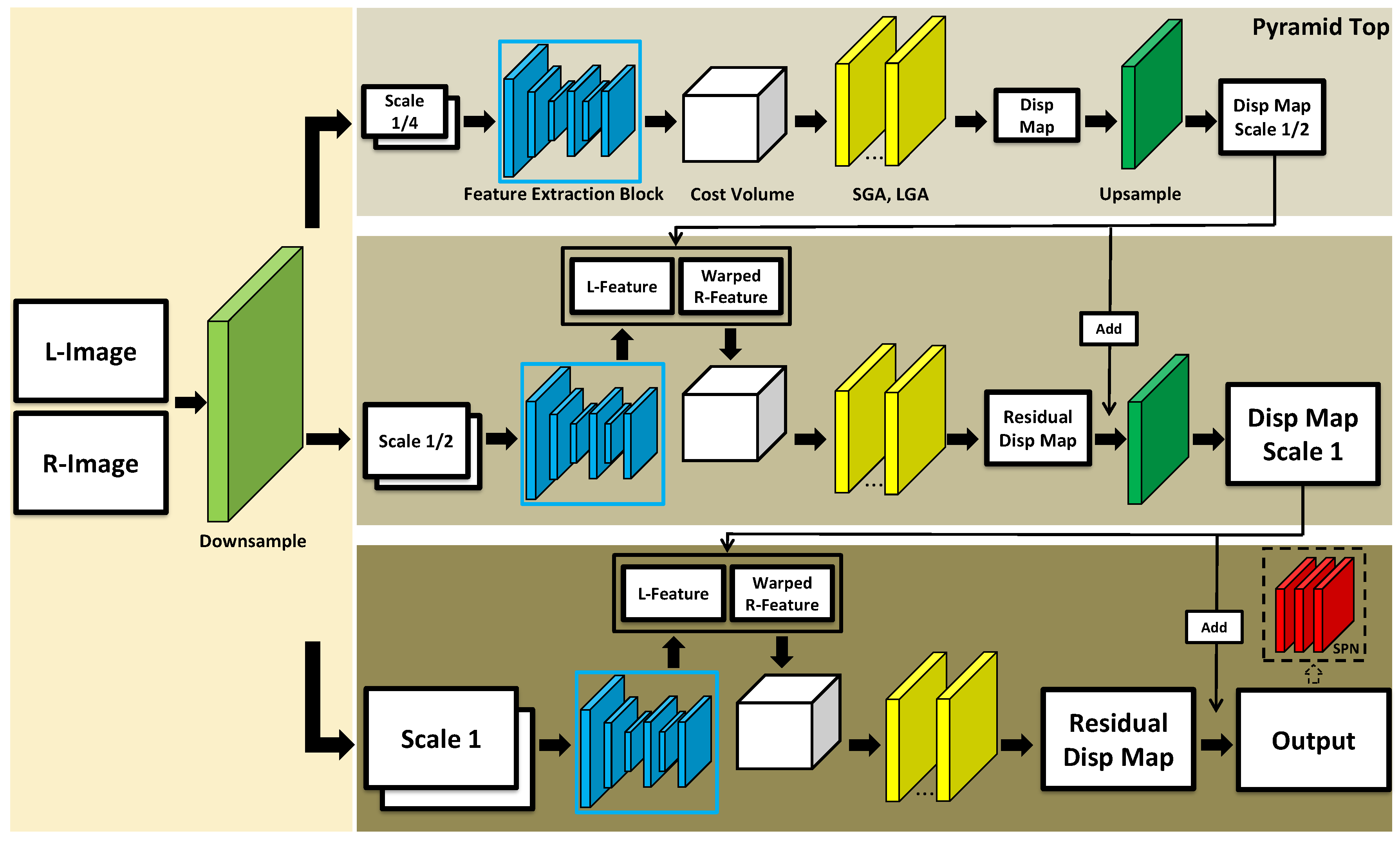

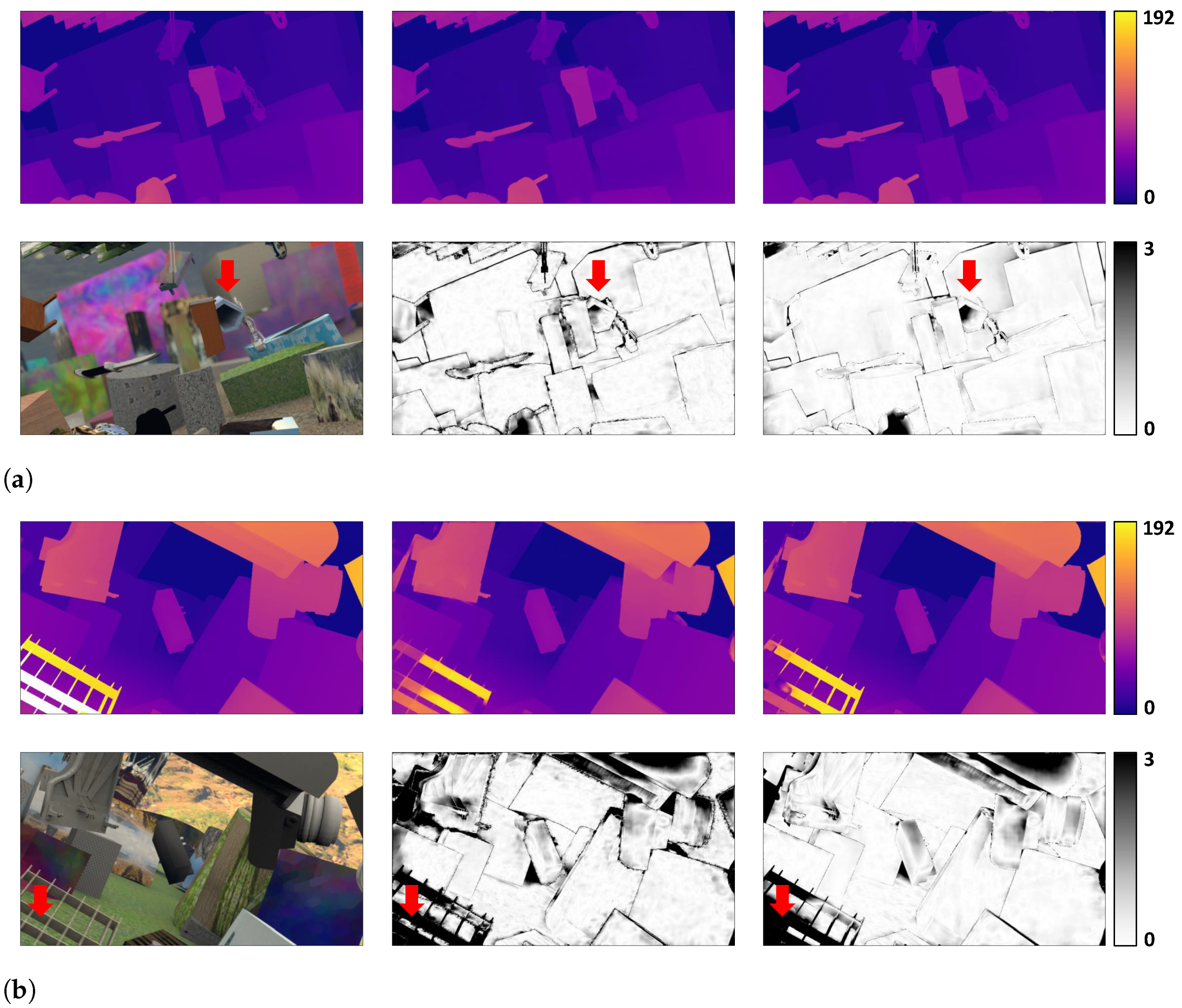
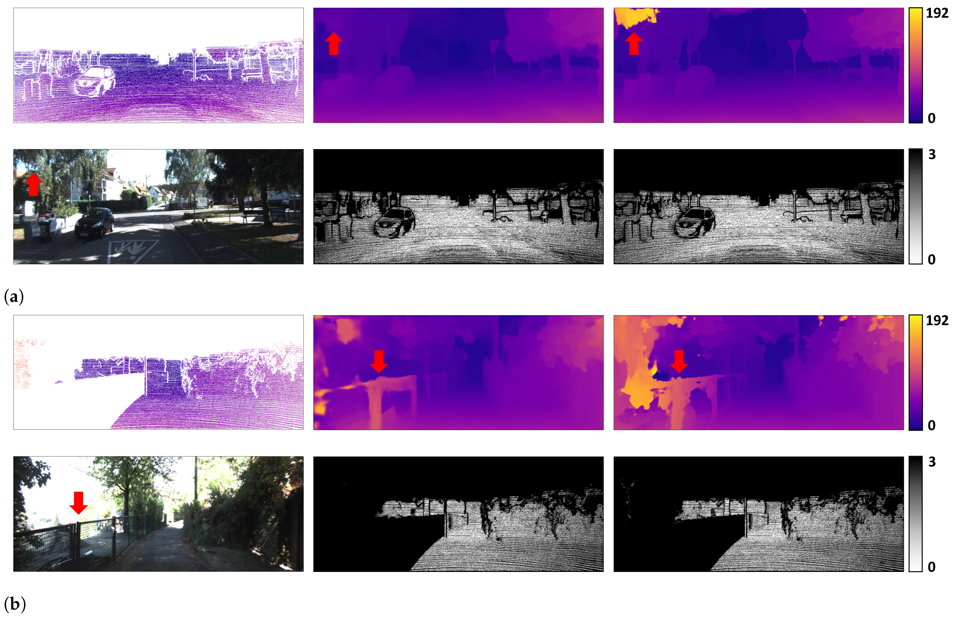
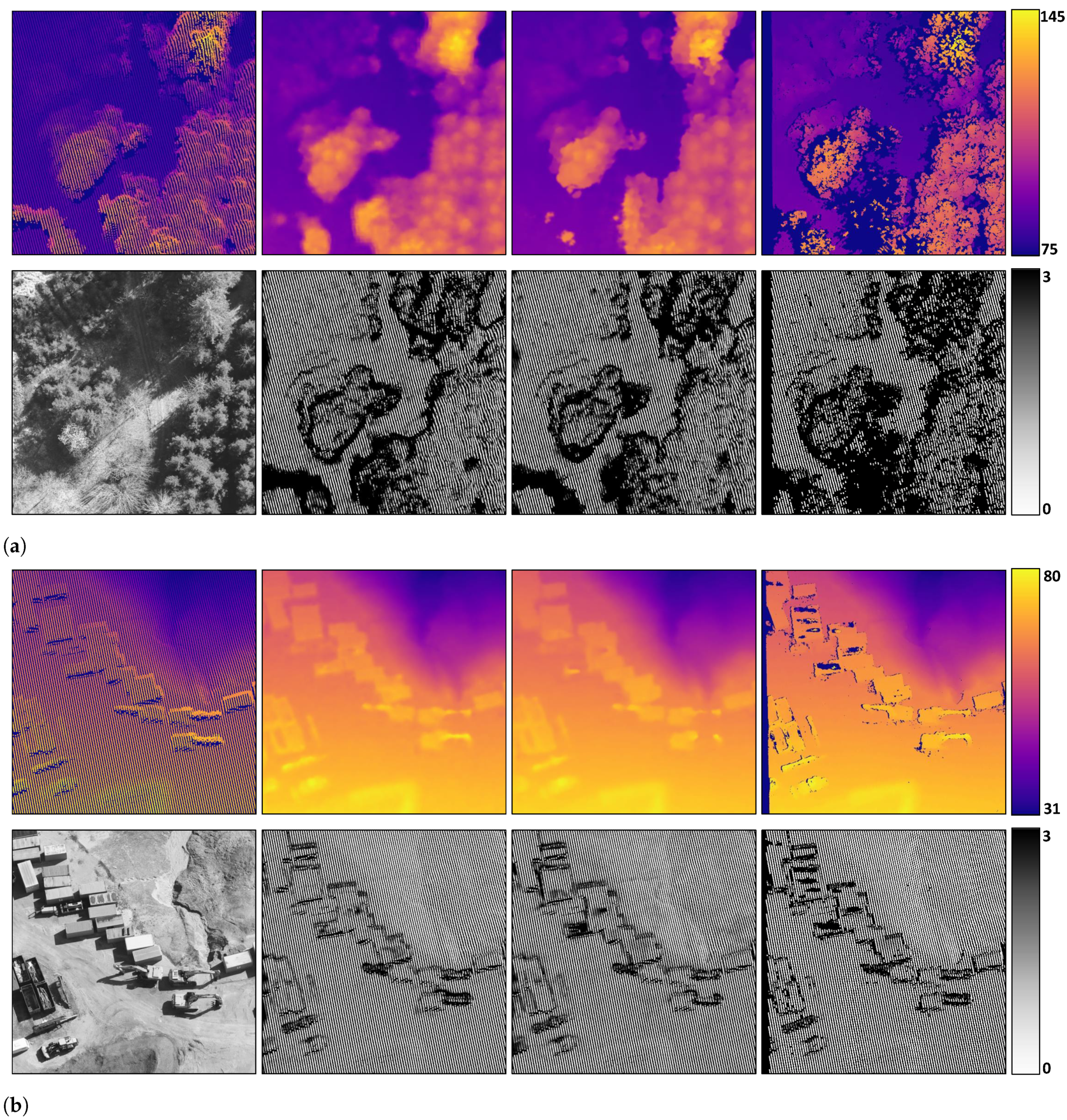
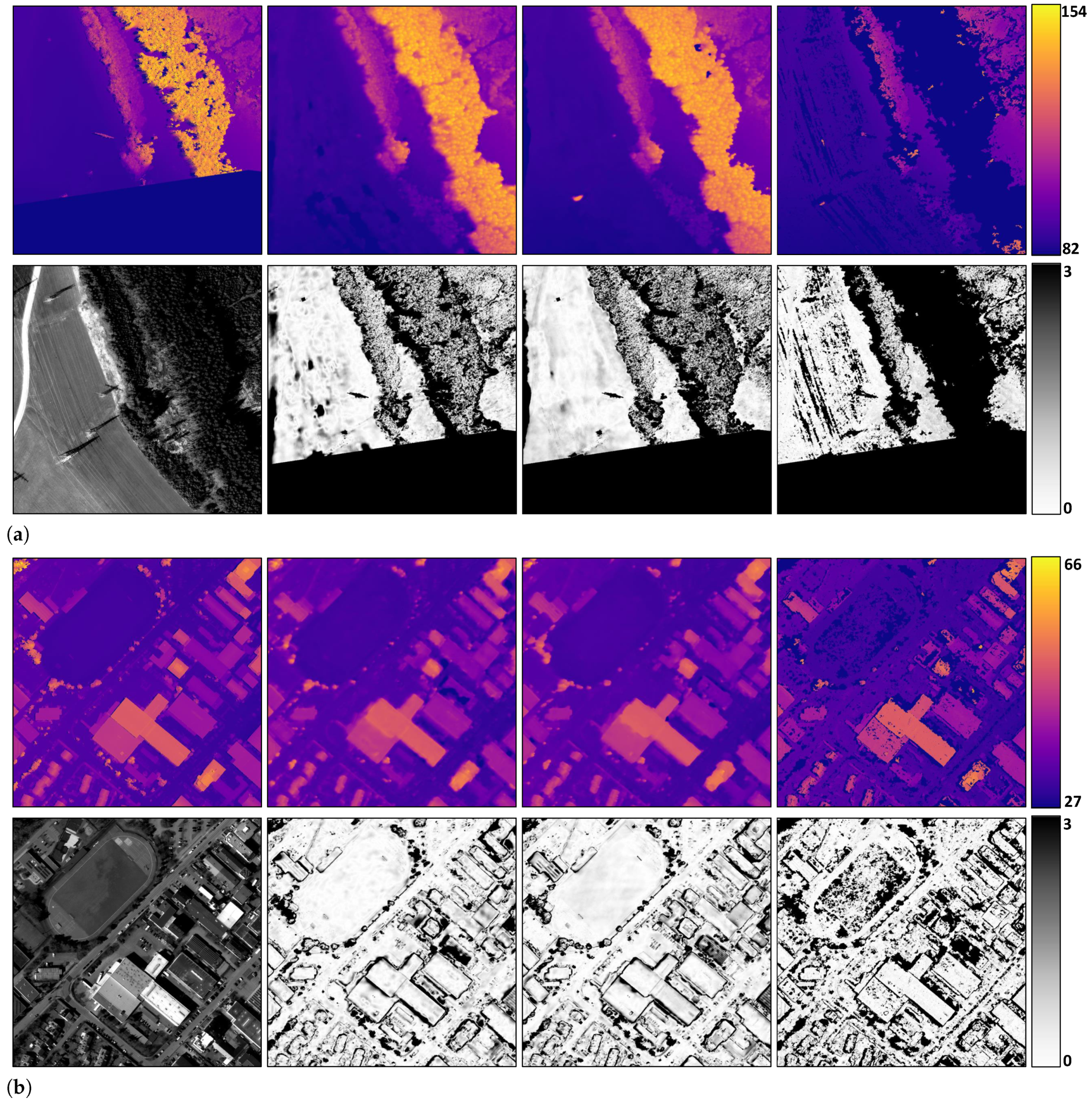

