Article

A Natural Images Pre-Trained Deep Learning Method for Seismic Random Noise Attenuation

1
School of Mathematics and Statistics, Xi’an Jiaotong University, Xi’an 710049, China
2
School of Information and Communications Engineering, Xi’an Jiaotong University, Xi’an 710049, China
*
Author to whom correspondence should be addressed.
Remote Sens. 2022, 14(2), 263; https://doi.org/10.3390/rs14020263
Submission received: 15 November 2021 / Revised: 21 December 2021 / Accepted: 2 January 2022 / Published: 7 January 2022

Abstract

:
Seismic field data are usually contaminated by random or complex noise, which seriously affect the quality of seismic data contaminating seismic imaging and seismic interpretation. Improving the signal-to-noise ratio (SNR) of seismic data has always been a key step in seismic data processing. Deep learning approaches have been successfully applied to suppress seismic random noise. The training examples are essential in deep learning methods, especially for the geophysical problems, where the complete training data are not easy to be acquired due to high cost of acquisition. In this work, we propose a natural images pre-trained deep learning method to suppress seismic random noise through insight of the transfer learning. Our network contains pre-trained and post-trained networks: the former is trained by natural images to obtain the preliminary denoising results, while the latter is trained by a small amount of seismic images to fine-tune the denoising effects by semi-supervised learning to enhance the continuity of geological structures. The results of four types of synthetic seismic data and six field data demonstrate that our network has great performance in seismic random noise suppression in terms of both quantitative metrics and intuitive effects.

1. Introduction

Seismic signals recorded by sensors onshore or offshore are usually contaminated by random noise, which leads to poor seismic data quality with low signal-to-noise ratio (SNR). Improving SNR of the seismic data is one of the targets of seismic data processing in which random noise suppression plays a key role in either pre-stack or post-stack seismic data processing.
There have been various denoising methods in recent decades such as prediction-based noise suppression method: t-x predictive filtering [1,2] and non-stationary predictive filtering [3,4], the sparse transform domain method including wavelet transform [5], curvelet transform [6], seislet transform [7], contourlets transform [8], dictionary learning-based sparse transform [9], singular spectrum analysis [10,11], etc. These traditional methods separate noise from signals mainly based on the features of signal and noise itself or their distribution characteristics in different transform domains. These methods usually require knowledge of prior information for the signal or the noise. Moreover, the features of seismic signals are complex in real situations and the distribution of characteristics of the signal and noise are overlapped in transform domain, so it is almost impossible to accurately separate the noise from noisy signals.
Recently, deep learning methods are popular and successfully deal with various tasks in different fields such as computer science, information engineering and earth science, and remote sensing. Deep learning methods have shown great potential for different tasks in the field of remote sensing such as image retrieval, road extraction, remote-sensing scene classification, semantic segmentation, and intelligent transport systems [12,13,14,15,16] as well as geophysics such as seismic inversion, interpretation, and seismic signal recognition [17,18,19,20,21,22,23,24,25,26,27,28,29,30,31]. In addition, deep learning approaches have also been successfully applied to suppress random noise in seismic data processing [18,32,33,34,35,36,37,38,39,40,41].
There are several classic deep learning methods for denoising. He et al. [42] presented a residual learning framework named ResNet (Deep Residual Network), which achieves an increase in the network depth without causing training difficulties. Compared with plain networks, ResNet adds a shortcut connection between every two layers to form residual learning. Residual learning solves the degradation problem of deep networks, allowing us to train deeper networks. Zhang et al. [43] proposed DnCNN (denoising convolutional neural network) for image denoising tasks based on the ideas of ResNet. The difference is that DnCNN does not add a shortcut connection every two layers like ResNet, but it directly changes the output of the network to a residual image. DnCNN learns the image residuals between the noisy image and the clean image. It can be converged quickly and has excellent performance under the condition of a deeper network. Ronneberger et al. [44] developed the U-net architecture, which consists of a contraction path and an expanding path. The common encoder–decoder structure is adopted, and skip connection is added to the original structure. It can effectively remain the edge detail information in the original image and prevent the loss of excessive edge information through up-sampling and down-sampling. Srivastava et al. [45] solved the overfitting problem which is difficult to deal with in deep learning by setting the dropout layers, that is, randomly discarding some units in the training process. Saad and Chen [46] proposed a new approach named DDAE (deep-denoising autoencoder) to attenuate seismic random noise. DDAE encodes the input seismic data into multiple levels of abstraction, then decodes them to reconstruct a noise-free seismic signal.
Contrary to many physical or model-based algorithms, the fully trained machine-learning algorithms have great advantages that they often do not need to specify any prior information (i.e., the signal or noise characteristics) or impose limited prior knowledge while they set multiple tuning parameters to obtain suitable results [40]. Consequently, the machine-learning algorithms are more user-friendly and offer possibly even fully automated applications. However, several factors determine the successfulness of the deep learning methods: (1) many more training examples must be provided than free parameters in the machine-learning algorithm avoiding the risk that the network memorizes the training data rather than learning the underlying trends [47,48]; (2) the provided training examples must be complete and the examples must span the full solution space [40].
In practice, deep neural networks usually have many hidden layers with thousands to millions of free parameters, thereby the requirement of more training examples than free parameters during training is often problematic and even unrealizable for geophysical applications. There are often two approaches to augment seismic training data. One is to use synthetic seismic data that is variable and easy to acquire the corresponding clean data. However, the synthetic data are not complete and representative generally, it is challenging for practical applications because the synthetic data do not contain all the features of the field data. The other strategy to augment training data is to use the preprocessing field data, but the trained network is unlikely to surpass the quality of the preprocessing training examples. Moreover, the clean data (ground truth) is unknown in complex geophysical applications.
The training examples are essential in deep learning methods, however, for the geophysical problems, the complete training data are not easy to be acquired especially for solving the actual problems. On the one hand, acquisition of seismic data is expensive and the field data is limited and complex, so the clean data is challenging to obtain. On the other hand, the synthetic seismic data can provide noise-free data but they cannot completely solve the problem of the field seismic data. It is well known that the natural images are available anywhere with abundant detail features. To solve the problem, several researchers have proven that the deep denoising network can be trained by the natural images and then it is likely to be capable of denoising the seismic data [49,50]. A similar strategy is to reconstruct images of black holes using a network trained with only natural images [51]. Zhang and van der Baan [40] proposed a generalization study for the neural networks to make the training examples complete and representative by using double noise injection and natural images. Double noise injection can increase the number of available training samples, which is more flexible for field data processing by training the algorithm to recognize and remove certain types of noise. Saad and Chen [38] proposed an unsupervised deep learning algorithm (PATCHUNET) to suppress random noise of seismic data with strategy of patching technique and skip connections. The proposed algorithm encodes the patched seismic data to extract the features of the input data and uses the decoder to map these extracted features to the clean signal without random noise.
In this work, we propose a new network architecture to suppress seismic random noise. Compared with previous work, the advancements of our new architecture are summarized as follows:
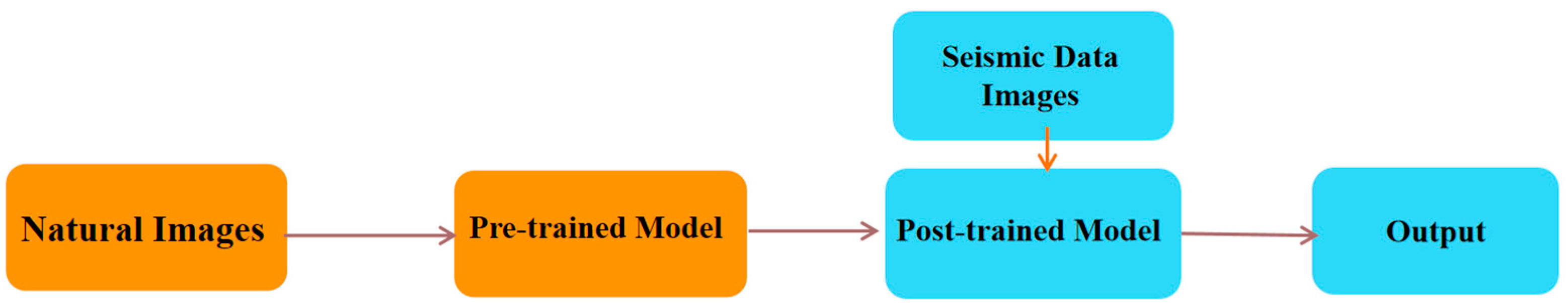
  • We treat the seismic data as an image throughout our network. Firstly, we train the network using exclusively natural images, then we transfer it to synthetic seismic image through the transfer learning. Secondly, we utilize the migrated seismic images to train a network different from the one used in the first step.
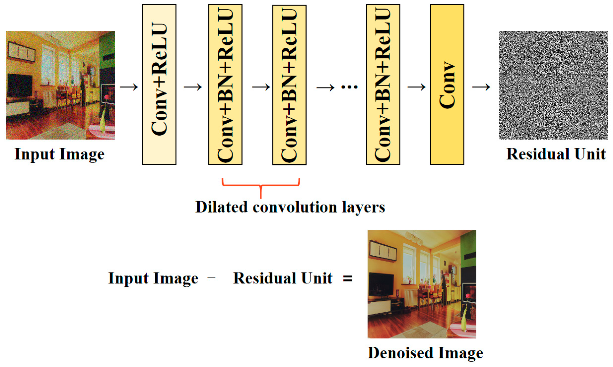
  • The dilated convolution is added in DnCNN to increase the size of the receptive field as well as to improve the training efficiency. This network is taken as a pre-trained network trained by only natural images.
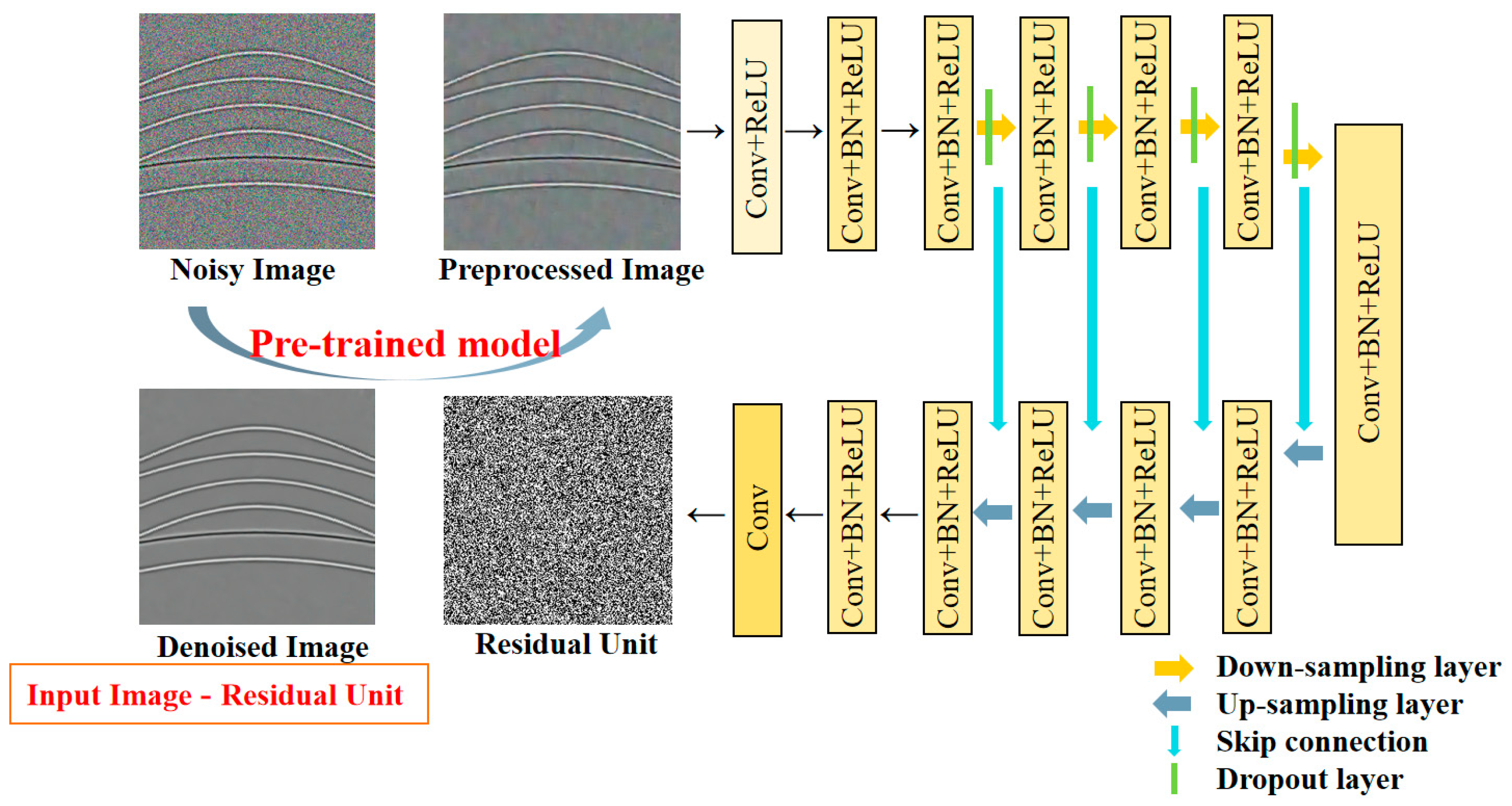
  • In order to fine-tune the denoising result of the pre-trained network, we design a post-trained network trained on synthetic seismic data in a way of semi-supervised learning. The network is the modified U-net with several dropout layers. We set the output of the network as a residual image to solve the difficulties of network training, in other words, the final denoised seismic images can be obtained by subtracting the output from the input.
This paper is organized as follows. In Section 2, we introduce the natural images pre-trained network for seismic random noise removal. In 
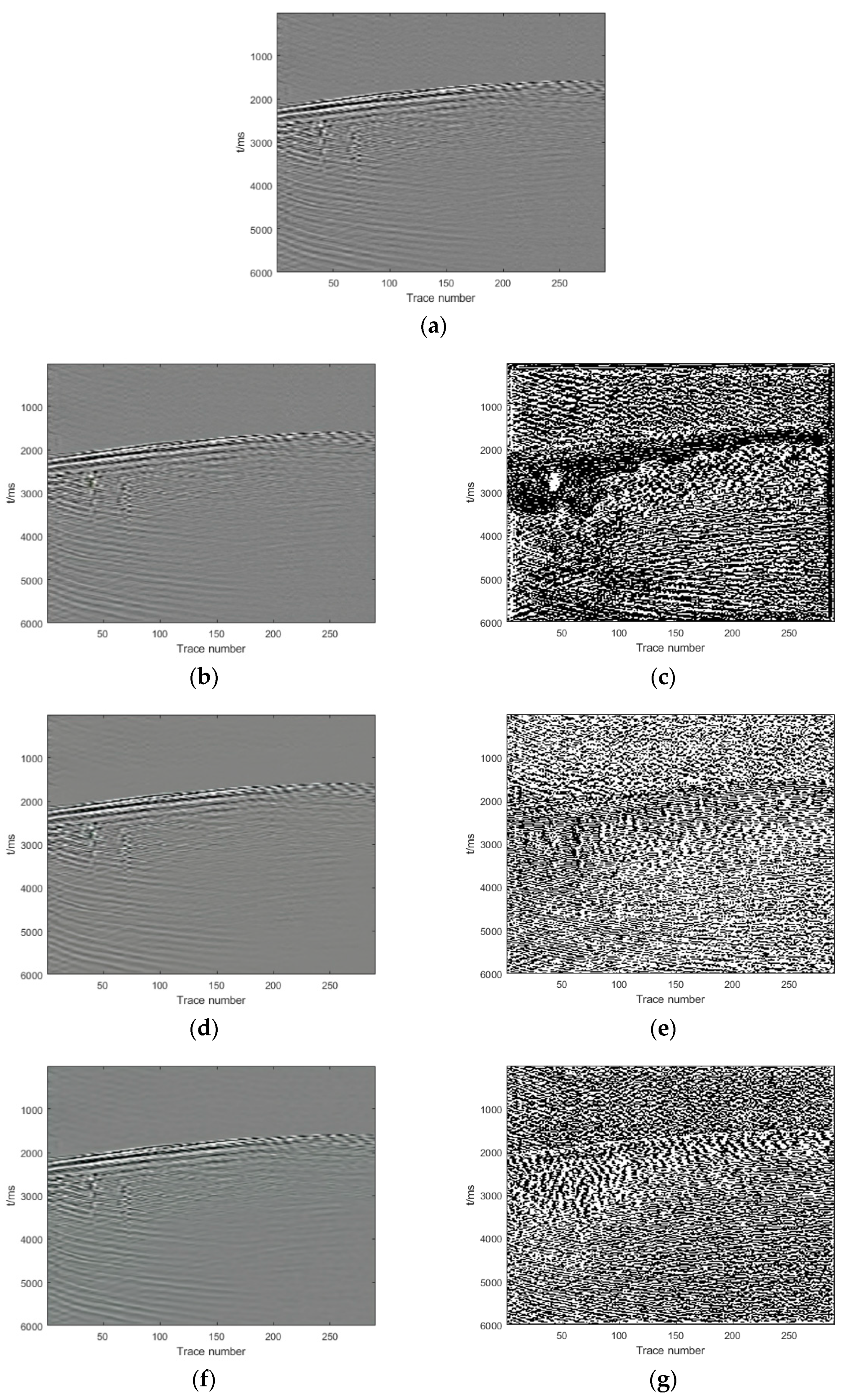
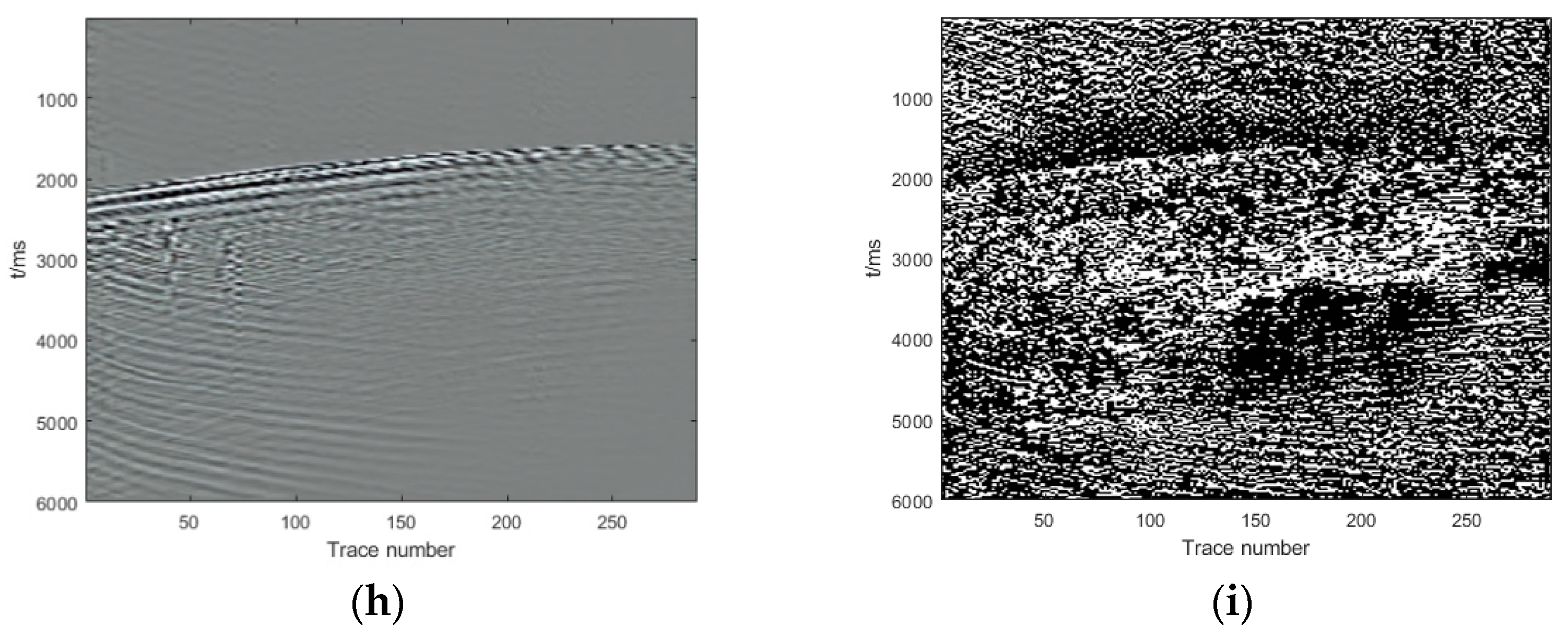
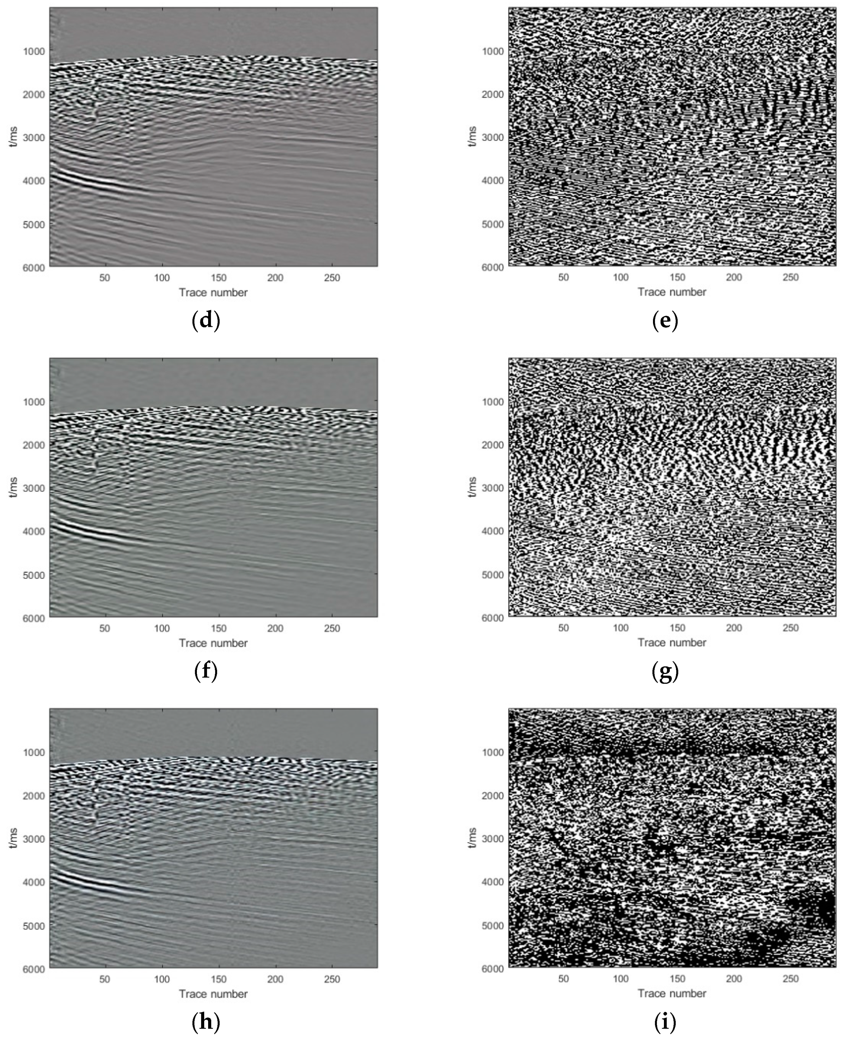
Section 3, we show and analyze the denoising results of four synthetic examples and six field examples comparing the denoising results with those obtained with DnCNN and U-net. Section 4 discusses the need for transfer learning and the importance of reasonable selection of parameters. Finally, we present a conclusion of this paper in Section 5.

2. Methods

We propose a new network architecture based on DnCNN and U-net for seismic random noise reduction. These two network architectures are combined through transfer learning. In the pre-trained network, we still follow the basic network architecture under the frame of DnCNN, but decrease the number of original network layers and utilize dilated convolution in the first few layers. Moreover, we add dropout layers and residual units in the U-net architecture as our post-trained network, which is different from the network in the first step, trained through the migrated seismic images.

2.1. Network Architecture

The whole denoising procedure is shown in Figure 1. The entire denoising network contains the pre-trained model and the post-trained model, both of which are connected by transfer learning. Firstly, we train the network using exclusively natural images (the specific dataset in Section 2.3) including scenery, people, animals, vehicles, etc. Then we transfer it to synthetic seismic image through transfer learning [52]. Secondly, we build a new network trained by minor amounts of seismic images to further restore the geological structures of seismic images. Throughout the denoising process, the noisy image is denoted as y, which is defined as
y = s + n
where s and n represent the clean image and the noise respectively. In addition, the noisy image y is the input of the network, and the output is the prediction of the clean image. We need to build a network so that the output is as close as possible to the corresponding clean image.

2.1.1. Pre-Trained Network: DnCNN with Dilated Convolution

The DnCNN is based on the structure of ResNet [42]. ResNet adds a shortcut connection between every two layers to form residual learning. The difference from ResNet is that DnCNN changes the output image of network to a residual image, instead of adding shortcut connection. This operation greatly improves the training efficiency, especially for images with low noise level.
In the pre-trained model, our network architecture is shown in Figure 2. The network depth is 13 layers with 32 convolution kernels. The size of the convolution kernel is 3. We use the rectified linear unit (ReLU) activation function after each hidden layer. The ReLU function can be expressed as
f ( x ) = { 0 , x 0 x , x > 0  
The output of middle layers requires additional batch normalization and is then activated. These operations are not implemented on the last layer.
Since the computational efficiency decreases with the depth of network increasing, we introduce the dilated convolution to increase the size of the receptive field without increasing the depth of the network. When the number of feature maps is the same, the dilated convolution can be utilized to get a larger receptive field. However, the continuous structural information may be lost at the same time, thus it is not conducive to the processing of details. Consequently, we only use dilated convolution in the second and third layers, and the dilated rate is set to 2. In this way, the network is allowed to better capture global features at the beginning of training.

2.1.2. Transfer Learning

Transfer learning is used to transfer the pre-trained model parameters to the new model training. Since most data or tasks are related, we can speed up the learning efficiency and optimize the model through this approach. For instance, natural images are ubiquitous in realistic life. The acquisition of seismic data requires a long time and financial resources, so we generally use synthetic seismic data to train the network. Compared to natural images, the seismic data have their own unique characteristics. Training using exclusively natural images will result in the loss of detailed seismic structure information. Therefore, we transfer the pre-trained model on natural images to a different network. This distinct network will be trained on seismic data. In this way, there is no need to restart the training of seismic data, which speeds up the training process. Specifically, we preserve the trained model parameters in the pre-trained model to implement preliminary denoising on the noisy seismic images. Then, these pre-processed seismic images are transferred to the post-trained model for retraining.

2.1.3. Post-Trained Network: U-Net Architecture with Residual Units and Dropout Layers

For seismic data training, we use U-net architecture with residual units and dropout layers (Figure 3). The input of the network is the pre-processed seismic image obtained through the pre-trained model. There are 13 convolutional layers in this network architecture. Except for the last layer, the output of each layer needs to be processed by batch normalization and is then activated with ReLU function. In addition, there are four down-sampling layers in the contraction path and corresponding four up-sampling layers in the symmetric expanding path, which are implemented by max-pooling and bilinear interpolation respectively. The size of the pool window, the up-sampling factor and the stride of each step are all set to 2. In the initial convolutional layer, the number of convolution kernels is 32. After each down-sampling layer except the last one, the number of convolutional filters doubles to 64, 128, and 256, respectively, then halves after every up-sampling operation except for the last layer. The dropout layers are added before each down-sampling layer to avoid overfitting. The dropout layer randomly reserves 90 percent of the parameters. Since the noise level of the image becomes lower after initial denoising in the first stage, we change the output to the residual image instead of the denoised image, which greatly increases the learning efficiency of the network.

2.2. Loss Function in Our Network

The whole denoising process can be described by the expression
s ^ = F 2 ( γ ; F 1 ( θ ; y ) )
where s ^ is the predicted image of the input image y from the proposed network architecture. F 1 ( θ ; y ) denotes the denoised image outputted from the DnCNN with dilated convolution. F 2 ( γ ; F 1 ( θ ; y ) ) refers to the denoised image outputted from the entire proposed network. Besides, θ and γ are the parameters of the DnCNN with dilated convolution and the U-net architecture with residual units respectively, including weights and biases.
We use different loss functions for the two training models. In the pre-trained model, the loss function is constructed in a supervised way, and in the post-trained model, a semi-supervised method is adopted.
Without loss of generality, the loss function in the pre-trained model is the averaged mean squared error between the clean seismic data and the denoised seismic data by the DnCNN with dilated convolution
min θ   l o s s 1 = 1 2 N i = 1 N s i F 1 ( θ ; y i ) F 2
The loss function of the post-trained model is determined as
min γ   l o s s 2 = α 1 2 N j = 1 N s j * F 2 ( γ ; F 1 ( θ ; y j * ) ) F 2 + 2 β 1 N j = 1 N SSIM ( s j * , y j * s ^ j * )
where { y i , s i } and { y j * , s j * }   ( i , j = 1 , , N ) denote N pairs of noise-clean training data from natural images and synthetic seismic data, respectively. Here, N refers to batch size. α and β are the weights measure the balance between the supervised and unsupervised learning. The loss function of averaged mean squared error is adopted in supervised learning, which is the same as the previous loss function. In unsupervised learning, the SSIM (structure similarity index measure) is utilized, which characterizes the structural similarity between the denoised seismic data and the removed noise. Adam optimizer is used to optimize the proposed network parameters [53].
The logarithm of loss curves in our methods are shown in Figure 4. Figure 4a,b indicate that the downward trend of the logarithm of the loss in the two networks is similar. The logarithm of loss drops sharply in the initial training stage, then decreases gradually. It is worth mentioning that the final convergence value of loss in the post-trained model is less than that in the pre-trained model, which further proves the necessity of the post-trained model. Furthermore, the loss is not divergent during the training process, illustrating that there is no over-fitting phenomenon in our networks. Regarding the choice of α and β in (5), we need to consider the trend of the loss curve under different α as well as the evaluation indexes of denoising results. Figure 4c illustrates the variation of the logarithm of loss curve with respect to α at different iteration steps in the post-trained model. Figure 4c shows that the logarithm of loss reaches the minimum at each certain iteration step when α = 0.9. In the following experiments, the evaluation indexes shows that the denoising result is the best with α = 0.9, β = 0.05 in the synthetic examples and α = 0.4, β = 0.3 in the field examples (clarified in details in Section 4.2).

2.3. Training Data Set Preparation

In order to apply our network architecture to seismic denoising, we prepare the training data set, including natural images and seismic images. The quantity of the training data sets allocations in the two models is shown in Table 1.
In deep learning, it is crucial to ensure the completeness of training data. Whether natural images or seismic images, we are supposed to ensure the diversity of data. We choose 1500 natural images for the first stage of training, 500 of which come from BSDS500 Dataset (website: https://eecs.berkeley.edu/ (accessed on 21 May 2021)) and the rest come from COCO Dataset (website: https://cocodataset.org/ (accessed on 28 June 2021)). There are various types of natural images in the two datasets, such as scenery, people, animals, vehicles, etc. In the second training stage, 1300 synthetic seismic images are used, 500 of which are VSP (Vertical Seismic Profile) data, the other 500 are the reflection seismic data, and the remaining are synthesized by the Marmousi2 model that is an open and one of the most representative geological models in the field of geophysics [54]. The geological structures of VSP data and the reflection seismic data are relatively simple, while the seismic data synthesized by Marmousi2 model is more complex. In this way, it can increase the richness of the seismic data and make the network more generalized.

2.3.1. VSP Data

The VSP method is a seismic survey technology in wells, in which seismic waves are excited at some points near the surface and they are received at the receivers in the well. According to the direction of propagation to the geophone, the seismic waves in the VSP data can be divided into down-going waves and up-going waves. The down-going waves have stronger energy, while the up-going waves are weaker. In our experiment, we use reflectivity method to generate VSP data in homogeneous layered models [55]. The VSP data are composed of random trace numbers from 151 to 501 and each with 2048 samples. The dominant frequency randomly varies from 10 to 60 Hz. The spacing of the geophones is 5 m. The sampling interval in time domain is 0.001 s.

2.3.2. Synthetic Reflection Seismic Data

We synthesize seismic reflection data through SeismicLab that is a MATLAB seismic data processing package (http://seismic-lab.physics.ualberta.ca/ (accessed on 2 June 2021)). The reflection seismic data are composed of different hyperbolic seismic events. To synthesize the reflection seismic data, we choose the dominant frequency of Ricker wavelet in the range of 10–40 Hz. The apparent velocity changes from 1500 to 2400 m/s. Consequently, we generate the clean synthetic reflection seismic data containing 101 traces and 901 samples. The sampling interval is 0.002 s.

2.3.3. Seismic Data Synthesized by Marmousi2 Model

We also obtain synthetic seismic data based on the Marmousi2 model (Figure 5). The Marmousi2 model has abundant geological structure which allows the network to learn more geological features. Part of them are calculated through convolution model, and the remaining part are acquired through the SEG open data (the website: https://wiki.seg.org/wiki/Open_data (accessed on 11 October 2021); data sets used: Kirchhoff_PoSDM.segy, Kirchhoff_PreSDM.segy, NMOstack_SRM.segy, SYNTHETIC.segy, WE_PreSDM.segy).
Next, we describe the principle of the convolution model briefly. Seismic records can be regarded as the convolution of a band-limited seismic wavelet and reflectivity series, which can be expressed as [56]
x ( t ) = w ( t ) r ( t )
where x ( t ) , w ( t ) , and r ( t ) represent seismic trace record, seismic wavelet, and reflectivity series, respectively.
Based on the Marmousi2 model, we generate seismic data using convolution method with Ricker wavelet. We choose the dominant frequency within the range of 10–40 Hz and the phase of the wavelet varies from 0–90 degrees. The sampling interval is 0.001 s. In this way, we generate seismic data containing 1701 traces and 1400 samples.
The seismic data generated by the Marmousi2 model are complex, so it is difficult to capture all the features if we input the entire synthetic data into the network directly. Therefore, we utilize the sliding window strategy to segment the synthetic seismic data and then input them into the network (shown in Figure 5). In the sliding window method [57], a window in size of 240 × 240 is slid over the seismic data from the top to the bottom and also from the left to the right with shift size of 180 samples. Each synthetic seismic data can produce 15 images through the sliding window strategy, then all the segment seismic images are input to the network for training.

2.3.4. Noise Injection

We add zero-mean discretized Gaussian white noise into all training data sets with 240 × 240 pixel randomly, and the standard deviation of noise ranges from 1 to 50 [43]. This value range is set to achieve the injection of strong noise and weak noise. We believe that the network can learn more characteristics of the noise if noise is added with different levels, thus the effective seismic signal can be restored more completely.

3. Results

We apply the proposed network to the synthetic seismic data to evaluate the denoising performance of our method and compare the results with those of the DnCNN and the U-net. Four synthetic examples are used to evaluate the proposed algorithm, including 255 seismic images obtained by VSP data, the reflection seismic data with hyperbolic events and Marmousi2 model. The synthesis method is the same as the training data sets. It is worth mentioning that the pre-stack Marmousi2 data (Kirchhoff_PreSTM_time.segy) in the test data sets is completely absent in the training set. Subsequently, random noise at different levels is added to the seismic images randomly. The quantity of the test data sets allocations is shown in Table 2.

3.1. Quantitative Analysis of Denoising Performance

In the following section, we use MSE (mean square error), PSNR (peak signal-to-noise ratio), and SSIM (structural similarity) as evaluation indexes of denoising performance. The MSE used here is calculated as
MSE = 1 N i = 1 N ( s i * s ^ i * ) 2
where s i * denotes the noise-free seismic data and s i * denotes the corresponding denoised seismic data.
The PSNR is defined as
PSNR = 10 log 10 ( 255 2 MSE )
and SSIM is described as
SSIM ( s i * , s ^ i * ) = l ( s i * , s ^ i * ) c ( s i * , s ^ i * ) s ( s i * , s ^ i * )
where l ( s i * , s ^ i * ) represents the brightness comparison, c ( s i * , s ^ i * ) is the contrast comparison, and s ( s i * , s ^ i * ) stands for the structure comparison [58].

3.2. Four Synthetic Examples

Experiments are carried out on four synthetic examples and six field examples to evaluate the denoising performance of the proposed method compared with two classic deep learning methods for seismic random noise attenuation. In addition to illustrating the superiority of our network through quantitative indicators mentioned above, we also testify this fact through visualization in the following.

3.2.1. First Synthetic Example (VSP Data)

We present the denoising results of VSP data as shown in Table 3 and Figure 6. The clean VSP data are shown in Figure 6a. Then the noisy data are generated by adding random noise with different levels, as illustrated in Figure 6b. This example contains strong down-going waves and weaker up-going waves. The original PSNR of the noisy data is 21.76.
The denoising sections of the pre-trained model with exclusively natural images are shown in Figure 6c. It is indicated that most of the noise have been removed through this pre-trained network, which corresponds to the greatly improved PSNR in Table 3. The PSNR of VSP data processed by the pre-trained network increases from 21.76 to 33.81. However, some weaker seismic events are lost and even disappeared, marked by the arrows in Figure 6c. Contrary to the preprocessed result, the noise-reduction results through our entire network are shown in Figure 6e. We find that the seismic events become more continuous and some detailed features are restored very clearly, especially in the parts marked by arrows in Figure 6e. The background of the whole image is also cleaner and brighter. At the same time, the evaluation indicators have been further improved. The denoised results of the DnCNN and U-net are illustrated in Figure 6g,i, respectively. Figure 6g,i indicate that the discontinuity on the up-going waves can be observed in the results of DnCNN and U-net, moreover, the PSNR and SSIM are lower than our proposed method while the MSE is larger than our method.
We illustrate the removed noise section between the original noisy data and the denoised data for all methods to further evaluate the denoising performance, as shown in Figure 6d,f,h,j. The down-going wave energy is exceedingly strong, so no matter which method is used to denoise, there will be different degrees of effective seismic signal damage. Both up-going and down-going coherent seismic waves are damaged in the pre-trained model, as shown in Figure 6d. Figure 6f clearly shows that the noisy section removed by our entire network contains extremely few up-going waves. However, both of DnCNN and U-net have up-going waves leakage to some extent, as shown in Figure 6h,j.
Table 3 indicates that the denoised data through the DnCNN and U-net has a PSNR of 36.09, 37.16 respectively, while the PSNR of the proposed method is 38.62. Furthermore, our method also has the lowest MSE and the highest SSIM among three methods.

3.2.2. Second Synthetic Example (Synthetic Reflection Seismic Data)

The synthetic reflection seismic data is used to appraise the proposed method. The seismic data contains six hyperbolic seismic events as shown in Figure 7a, while the noisy data are presented in Figure 7b. As shown in Figure 7c, the denoised data obtained by pre-trained model contains clutter in the background but little random noise, some signal loss is visible in the removed noise section (Figure 7d). By comparison, the random noise is removed completely and messy background is improved through further processing of the post-trained model, as shown in Figure 7e. Furthermore, the removed noise section (Figure 7f) has no signal leakage basically. Judging from the denoised results with the DnCNN (Figure 7g) and U-net (Figure 7i), their denoising performance is not bad. However, there is still signal leakage, as can be seen from the removed noise section (Figure 7h,j). From the evaluation index values in Table 4, our proposed method achieves the best denoising performance compared with the other two methods, especially in our method the SSIM is as high as 0.99 while PSNR is up to 39.52. The results demonstrate that the proposed method effectively removes random noise while reserving the hyperbolic seismic events.

3.2.3. Third Synthetic Example (Marmousi2 Model Data)

We utilize synthetic seismic data by the Marmousi2 model (calculated through convolution model) to assess the proposed method. Similar to the training set, we process them through the sliding window method before using them for testing. Figure 8a,b show the clean data and noisy data, respectively. The pre-trained model only removes most of the random noise (Figure 8c), but many detailed features of Marmousi2 model are not retained. The same result can be obtained from the difference profiles (Figure 8d). The denoised and the removed noise section by the proposed method are shown in Figure 8e,f, respectively. In contrast with the denoised section of the pre-trained model, the post-trained model after transfer learning recovers many detailed geological features and weak seismic signals. The seismic signals reconstructed by the DnCNN (Figure 8g) and U-net (Figure 8i) are blurry with a lot of interferences. The signal leakage obviously exists in the difference map (Figure 8h,j), especially for the DnCNN. The apparent signal leakage in all difference profiles are marked with rectangular boxes.
As listed in Table 5, the DnCNN and U-net have poor denoising performance on Marmousi2 data, while our method still performs well. The PSNR and SSIM of our network are 37.77 and 0.95, respectively, and the MSE is as low as 0.000207.

3.2.4. Fourth Synthetic Example (the Pre-Stack Marmousi2 Data)

Finally, we test the proposed method on pre-stack Marmousi2 data as shown in Figure 9a. The data contains various complex geological features but does not participate the network training. We add random noise to the pre-stack data, as shown in Figure 9b. The denoised sections with pre-trained model and the proposed method are respectively shown in Figure 9c,e. Figure 9c,e indicate that both models can effectively suppress random noise. We zoom in the parts of the denoising result to clearly show the performance of the pre-trained and post-trained network, as illustrated on the left side of Figure 9c,e. We find that many weak seismic signals marked with the red rectangle in the enlarged parts are removed as random noise in the pre-trained model, while they are well restored in the post-trained model. However, the seismic signals after denoising by the pre-trained model damage in blocks, which can also be seen from the difference map (Figure 9d). On the contrary, in the difference map after denoising by our entire model (Figure 9f), such phenomenon is barely noticeable, only a few detailed features are lost, while most of the signals are well reserved. In the DnCNN and U-net, the denoised images (Figure 9g,i) have point-like blur, which indicates that both networks do not capture the detailed features of the seismic signals. Although only little signal leakage can be seen intuitively from the removed noise section (Figure 9h,j) for the DnCNN and U-net, it does not mean that they have excellent denoising performance. The corresponding conclusion can be obtained in Table 6. The U-net has the equally high SSIM as our method, but it is more convincing based on all the three evaluation indexes. Consequently, the proposed method outperforms the other two methods in preserving the seismic signals and reducing the random noise.
Table 7 lists the MSE, PSNR, and SSIM of the results by using the pre-trained model, the proposed method, the DnCNN and the U-net averaged by all the test data sets. It can be seen that, in contrast to other methods, the proposed method has the larger PSNR value, SSIM value and lower value of MSE. This indicates that our method has better denoising performance than other two methods. In terms of evaluation indexes, the denoising performance of the U-net is inferior, and the DnCNN is the worst. Moreover, each evaluation index has been improved appropriately through the pre-trained model, which also demonstrates the necessity of this model. The result also confirms our previous idea. It is feasible to use natural images for pre-training and then be applied in seismic noise attenuation.

3.3. Field Example Application

To further demonstrate the denoising performance of the proposed method, the network is applied to the CDP multichannel seismic profiles (website: https://wiki.seg.org/wiki/Open_data (accessed on 11 October 2021); specific data set: U121_01.SGY). We compare the proposed method with the DnCNN and U-net. The noisy data is shown in Figure 10a, and there is no clean data. We can see that a large amount of other types of noise exist in the seismic data in addition to the random noise. The denoised data and the different profiles obtained through the pre-trained model and proposed method are illustrated in Figure 10b–e, respectively. It can be seen that there is still some random noise in the denoised result of the pre-trained model. The same phenomenon is found in the denoised results of the DnCNN and U-net, as shown in Figure 10f–i. Relatively, the denoised data after post-trained model is less noisy.
The field seismic data is too noisy, so it is difficult to see the obvious difference through the denoised data. Furthermore, we analyze the denoising performance in the difference profiles. The pre-trained model regards some useful seismic signals as noise, which results in various degrees of signal loss. The obvious seismic signal leakage appears in the DnCNN and U-net as shown in Figure 10g,i. On the contrary, the signal leakage of proposed method is lower than the DnCNN and U-net. The field seismic example demonstrates that the proposed method is applicable in terms of effectively removing the random noise and reserving seismic signals.
To further demonstrate the applicability of our method, it is not enough to show a single field example of denoising. The proposed method is aimed at applying to field seismic data, so we test the method on several field examples with different seismic data types additionally and compare the denoising results with the DnCNN and U-net. The denoising results of the field VSP data are shown in Figure 11, Figure 12 and Figure 13 respectively. These VSP data not only contain random noise, but also are contaminated by other more complex noise. As shown in Figure 11b, Figure 12b and Figure 13b, there is still a large amount of random noise in the denoising result of the pre-trained model. However, the random noise is largely removed and the seismic signals are well preserved after further processing of the post-trained model. The DnCNN is almost comparable to our method in terms of eliminating random noise, but the noise removal in DnCNN is not complete enough in the part of weak signals. The denoising effect of U-net is not as good as DnCNN and our method because it damages many signals, as illustrated in the difference profiles in Figure 11, Figure 12 and Figure 13.
In addition, the two post-stack field seismic data are also tested as shown in Figure 14 and Figure 15. The overall denoising results on these post-stack field data are the same as the results of VSP data mentioned above. Although a lot of random noise can be removed through U-net, poor continuity is manifested in seismic events. The noise attenuation by DnCNN is incomplete. Many cases of signal loss and incomplete denoising exist in the results of the pre-trained model. Obviously, the seismic signals are relatively recovered and have good lateral continuity after the post-trained model. Especially for the sixth field seismic data, our method can reserve more signals relatively compared with other networks. The results of the six field seismic data illustrate that our method achieves a good tradeoff between random noise attenuation and effective signal preservation. Furthermore, the denoising results of both synthetic and field data demonstrate that a post-trained model is important and necessary in the process of denoising.

3.4. Training Time Comparison

In order to validate the advantages of our network architecture and the effectiveness of transfer learning, we compare it with the DnCNN and U-net in terms of training time. We train the network through NVIDIA GeForce RTX 2080 Ti GPU. In DnCNN and U-net training, we use their original network architecture without any changes, and inject all training data into the network at once. In order to ensure the fairness of comparison, the number of network layers is consistent with our network. The training time are recorded in Table 8. Comparing with the DnCNN and U-net, it can be seen that the training time of our method is shorter, as shown in Table 8. The comparison result indicates that transfer learning greatly improves training speed of our network architecture. This is because we do not need to input natural images and seismic data into the network simultaneously for training.

4. Discussion

4.1. Necessity of Transfer Learning

The denoising results of four synthetic seismic data and six field data mentioned above imply that the pre-trained model trained only by the natural images can remove most of the random noise in the data. It explains that we can treat seismic images as a subclass of natural images then perform pre-trained network on noisy seismic data, which provides an essential approach for seismic data augmentation. However, due to the poor processing of details, weak seismic signals disappear and become blurred in the pre-trained network. Subsequently, the seismic data are applied to train the post-trained model to fine-tune the denoising result in a semi-supervised learning. The PSNR, SSIM, and MSE are then greatly improved, and many complex geological features are well restored. On the other hand, the denoising process shows that seismic data also has its own unique features that are different from the natural images. The pre-trained network can provide preliminary denoising results, but it is unable to learn some detailed geological structures in the seismic data if it is trained by only natural images.
In terms of computational efficiency, transfer learning can sequentially input natural images and seismic images into different networks, instead of inputting them into one network at once for training like the DnCNN and U-net. This greatly reduces training time and the complexity of network training. Moreover, the network can be trained purposefully, that is, the pre-trained model is used to denoise roughly, then the post-trained model is to fine-tune the denoising result to further restore the detailed characteristics of the seismic signals.

4.2. Loss Function Parameters Selection in Post-Trained Model

In the post-trained model, the loss function is defined in a semi-supervised way; that is, a combination of MSE and SSIM. The MSE means the difference between the clean data and the denoised data, while the SSIM measures the similarity between the denoised data and the noise removed. However, the weights on MSE and SSIM must be measured based on the different characteristics of seismic data in order to achieve the best denoising performance. In other words, different weights should be applied for the data with simple and complex geological structures.
Firstly, we determine the optimal weight for four synthetic examples through many experiments, as show in Table 9. The synthetic examples have simple geological structures with only random noise added manually. We find that the results of evaluation indexes will be worse if the two weights approach the same. When the two weights are different greatly, the denoising performance will be better. It indicates that in the synthesis examples, one is used as the main control factor and the other act as the fine-tuning factor in the loss function, consequently the effect of denoising is reasonable and satisfactory. In fact, the network only using MSE as the loss function can still achieve great denoising performance, but seismic events become more continuous and clearer after fine-tuning by SSIM. We finally choose the weight α = 0.9 and β = 0.05 with the best metrics in our experiments.
Secondly, the field example with complex geological structures contains strong interferences, not just the random noise. We also implement the experiments with different weights that are the same as Table 9, and some representative denoising results are presented in Figure 16a–h. Either from the denoised data or the difference profiles, it can be indicated that a large amount of random noise is removed under the combination of four pairs of parameters. Generally, the leakage of seismic signals gradually decreases as β increases. However, the large value of β will also cause a degree of seismic signal loss. Therefore, we choose α = 0.4 and β = 0.3 as the best match in our field experiment. It can be clearly observed from the difference profiles that the leakage of seismic signals is minimal when the parameters are chosen as this combination. Accordingly, β cannot be too small for the complex field example, thus the SSIM index plays an important role in reserving the geological structures in the field data.

4.3. Quantitative ‘Stress Test’ for the Synthetic Examples

We randomly add Gaussian white noise with different levels to all synthetic seismic data to evaluate the performance of our method in Section 3.2. However, the denoising performance of our method for a certain noise level is not analyzed and evaluated. In this part, we perform a quantitative ‘stress test’ on synthetic examples to highlight this problem. We implement the denoising task for different noise levels in which the different standard deviations from 10 to 70 in noise injection are chosen as different noise levels. Then three evaluation indexes are adopted to analyze the denoising performance of our method under different noise levels. All experimental results are shown in Table 10. It is indicated that our method has better denoising performance on seismic images with weaker noise levels. In the training examples, the maximum standard deviation of the Gaussian noise distribution is 50, but the larger standard deviations are chosen for testing in the ‘stress test’. It is indicated that our method still works when the noise level is beyond the noise level during training, and it exerts relatively satisfying denoising performance.

5. Conclusions

A natural images pre-trained deep learning method is proposed to suppress seismic random noise through insight of the transfer learning. Our proposed network contains two networks: pre-trained and post-trained networks. The former is DnCNN with the dilated convolution trained with natural images exclusively. The latter is similar to U-net trained with a relatively small number of seismic images in a way of semi-supervised learning, in which the dropout layers are added and the output is changed to the residual image.
We use transfer learning to achieve seismic image denoising through pre-training on natural images. The PSNR, MSE, and SSIM of the pre-trained network have been greatly improved in the first stage, but some details of the seismic events are not processed well enough. Compared with natural images, seismic images have their own unique characteristics. Then we utilize transfer learning to transfer the trained network to the post-trained network. In the second section, we continue to train the post network on seismic data to adjust the denoising results by combining the MSE and SSIM in a way of semi-supervised learning to restore the geological structures in seismic data. The final denoised results on synthetic seismic data and field data show that the pre-trained network can provide preliminary denoising results and many detailed structure features of seismic data are better restored through the fine tuning of the post-trained network. Our network has better performance in seismic random noise suppression than the other two classic methods in terms of quantitative metrics and intuitive effects, as well as training efficiency.

Author Contributions

All the authors made significant contributions to this work. H.Z. and T.B. designed the framework of the network and performed the experiments; T.B. and Z.W. prepared the training data set; H.Z., T.B. and Z.W. analyzed the results; T.B. and H.Z. wrote the paper; H.Z. acquired the funding support. All authors have read and agreed to the published version of the manuscript.

Funding

This research was funded by the National Natural Science Foundation of China under grant no. 41974132 and National Key R&D Program of China under grant no. 2021YFA0716901.

Institutional Review Board Statement

Not applicable.

Informed Consent Statement

Not applicable.

Data Availability Statement

The natural images of BSDS500 Dataset and COCO Dataset are obtained from https://eecs.berkeley.edu/ (accessed on 21 May 2021) and https://cocodataset.org/ (accessed on 28 June 2021), respectively. Part of synthetic seismic data and field data come from SEG open data (website: https://wiki.seg.org/wiki/Open_data (accessed on 11 October 2021)).

Acknowledgments

The authors would like to thank SEG and Gary S. Martin et al. for the open model: Marmousi2 and the open data. We would also like to thank the natural image dataset of BSDS500 Dataset and COCO Dataset and the open source code of U-net (https://github.com/jakeret/tf_unet (accessed on 10 August 2021)) and DnCNN (https://github.com/wbhu/DnCNN-tensorflow (accessed on 2 May 2021)) as well as SeismicLab package (http://seismic-lab.physics.ualberta.ca/ (accessed on 2 June 2021)).

Conflicts of Interest

The authors declare no conflict of interest.

References

  1. Abma, R.; Claerbout, J. Lateral prediction for noise attenuation by t-x and f-x techniques. Geophysics 1995, 60, 1887–1896. [Google Scholar] [CrossRef] [Green Version]
  2. Gulunay, N. Noncausal spatial prediction filtering for random noise reduction on 3-D poststack data. Geophysics 2000, 65, 1641–1653. [Google Scholar] [CrossRef]
  3. Liu, G.; Liu, Y.; Li, C.; Chen, X. Weighted Multisteps Adaptive Autoregression for Seismic Image Denoising. IEEE Geosci. Remote Sens. Lett. 2018, 15, 1342–1346. [Google Scholar] [CrossRef]
  4. Liu, G.; Chen, X.; Du, J.; Wu, K. Random noise attenuation using f-x regularized nonstationary autoregression. Geophysics 2012, 77, V61–V69. [Google Scholar] [CrossRef]
  5. Anvari, R.; Siahsar, M.A.N.; Gholtashi, S.; Kahoo, A.R.; Mohammadi, M. Seismic Random Noise Attenuation Using Synchrosqueezed Wavelet Transform and Low-Rank Signal Matrix Approximation. IEEE Trans. Geosci. Remote Sens. 2017, 55, 6574–6581. [Google Scholar] [CrossRef]
  6. Liu, W.; Cao, S.; Chen, Y.; Zu, S. An effective approach to attenuate random noise based on compressive sensing and curvelet transform. J. Geophys. Eng. 2016, 13, 135–145. [Google Scholar] [CrossRef] [Green Version]
  7. Liu, Y.; Fomel, S.; Liu, C. Signal and noise separation in prestack seismic data using velocity-dependent seislet transform. Geophysics 2015, 80, WD117–WD128. [Google Scholar] [CrossRef] [Green Version]
  8. Zhao, X.; Li, Y.; Zhuang, G.; Zhang, C.; Han, X. 2-D TFPF based on Contourlet transform for seismic random noise attenuation. J. Appl. Geophys. 2016, 129, 158–166. [Google Scholar] [CrossRef]
  9. Zu, S.; Zhou, H.; Wu, R.; Jiang, M.; Chen, Y. Dictionary learning based on dip patch selection training for random noise attenuation. Geophysics 2019, 84, V169–V183. [Google Scholar] [CrossRef]
  10. Huang, W.; Wang, R.; Chen, Y.; Li, H.; Gan, S. Damped multichannel singular spectrum analysis for 3D random noise attenuation. Geophysics 2016, 81, V261–V270. [Google Scholar] [CrossRef]
  11. Oropeza, V.; Sacchi, M. Simultaneous seismic data denoising and reconstruction via multichannel singular spectrum analysis. Geophysics 2011, 76, V25–V32. [Google Scholar] [CrossRef]
  12. Zhu, X.X.; Tuia, D.; Mou, L.; Xia, G.-S.; Zhang, L.; Xu, F.; Fraundorfer, F. Deep Learning in Remote Sensing. IEEE Geosci. Remote Sens. Mag. 2017, 5, 8–36. [Google Scholar] [CrossRef] [Green Version]
  13. Abdollahi, A.; Pradhan, B.; Shukla, N.; Chakraborty, S.; Alamri, A. Deep Learning Approaches Applied to Remote Sensing Datasets for Road Extraction: A State-Of-The-Art Review. Remote Sens. 2020, 12, 1444. [Google Scholar] [CrossRef]
  14. de Lima, R.P.; Marfurt, K. Convolutional Neural Network for Remote-Sensing Scene Classification: Transfer Learning Analysis. Remote Sens. 2020, 12, 86. [Google Scholar] [CrossRef] [Green Version]
  15. Xu, Z.; Zhang, W.; Zhang, T.; Li, J. HRCNet: High-Resolution Context Extraction Network for Semantic Segmentation of Remote Sensing Images. Remote Sens. 2021, 13, 71. [Google Scholar] [CrossRef]
  16. Jingrui, L.; Jinbo, L.; Guangde, Y. Seatbelt detection in road surveillance images based on improved dense residual network with two-level attention mechanism. J. Electron. Imaging 2021, 30, 033036. [Google Scholar]
  17. Huang, W.-L.; Gao, F.; Liao, J.-P.; Chuai, X.-Y. A deep learning network for estimation of seismic local slopes. Pet. Sci. 2021, 18, 92–105. [Google Scholar] [CrossRef]
  18. Zhang, Z.-D.; Alkhalifah, T. Regularized elastic full-waveform inversion using deep learning. Geophysics 2019, 84, R741–R751. [Google Scholar] [CrossRef]
  19. Wang, Y.; Ge, Q.; Lu, W.; Yan, X. Seismic impedance inversion based on cycle-consistent generative adversarial network. In SEG Technical Program Expanded Abstracts 2019; Society of Exploration Geophysicists: Tulsa, OK, USA, 2019; pp. 2498–2502. [Google Scholar]
  20. Zhang, Z.; Lin, Y. Data-Driven Seismic Waveform Inversion: A Study on the Robustness and Generalization. IEEE Trans. Geosci. Remote Sens. 2020, 58, 6900–6913. [Google Scholar] [CrossRef] [Green Version]
  21. Wu, B.; Meng, D.; Wang, L.; Liu, N.; Wang, Y. Seismic Impedance Inversion Using Fully Convolutional Residual Network and Transfer Learning. IEEE Geosci. Remote Sens. Lett. 2020, 17, 2140–2144. [Google Scholar] [CrossRef]
  22. Pan, W.; Torres-Verdin, C.; Pyrcz, M.J. Stochastic Pix2pix: A New Machine Learning Method for Geophysical and Well Conditioning of Rule-Based Channel Reservoir Models. Nat. Resour. Res. 2020, 30, 1319–1345. [Google Scholar] [CrossRef]
  23. Jo, H.; Santos, J.E.; Pyrcz, M.J. Conditioning well data to rule-based lobe model by machine learning with a generative adversarial network. Energy Explor. Exploit. 2020, 38, 2558–2578. [Google Scholar] [CrossRef]
  24. Mustafa, A.; AlRegib, G. Joint learning for seismic inversion: An acoustic impedance estimation case study. In SEG Technical Program Expanded Abstracts 2020; Society of Exploration Geophysicists: Tulsa, OK, USA, 2020; pp. 1686–1690. [Google Scholar]
  25. Li, S.; Liu, B.; Ren, Y.; Chen, Y.; Yang, S.; Wang, Y.; Jiang, P. Deep-Learning Inversion of Seismic Data. IEEE Trans. Geosci. Remote Sens. 2020, 58, 2135–2149. [Google Scholar] [CrossRef] [Green Version]
  26. Wang, B.; Zhang, N.; Lu, W.; Wang, J. Deep-learning-based seismic data interpolation: A preliminary result. Geophysics 2019, 84, V11–V20. [Google Scholar] [CrossRef]
  27. Huang, W. Seismic signal recognition by unsupervised machine learning. Geophys. J. Int. 2019, 219, 1163–1180. [Google Scholar] [CrossRef]
  28. Liu, N.; He, T.; Tian, Y.; Wu, B.; Xu, Z. Common azimuth seismic data fault analysis using residual U-Net. Interpretation 2020, 8, 1–41. [Google Scholar] [CrossRef]
  29. Wang, Z.; Li, B.; Liu, N.; Wu, B.; Zhu, X. Distilling knowledge from an ensemble of convolutional neural networks for seismic fault detection. IEEE Geosci. Remote Sens. Lett. 2020, 19, 1–5. [Google Scholar] [CrossRef]
  30. Qiu, C.; Wu, B.; Liu, N.; Zhu, X.; Ren, H. Deep Learning Prior Model for Unsupervised Seismic Data Random Noise Attenuation. IEEE Geosci. Remote Sens. Lett. 2021, 19, 1–5. [Google Scholar] [CrossRef]
  31. Wu, B.; Meng, D.; Zhao, H. Semi-Supervised Learning for Seismic Impedance Inversion Using Generative Adversarial Networks. Remote Sens. 2021, 13, 909. [Google Scholar] [CrossRef]
  32. Zhang, Y.; Lin, H.; Li, Y.; Ma, H. A Patch Based Denoising Method Using Deep Convolutional Neural Network for Seismic Image. IEEE Access 2019, 7, 156883–156894. [Google Scholar] [CrossRef]
  33. Zhao, Y.; Li, Y.; Dong, X.; Yang, B. Low-Frequency Noise Suppression Method Based on Improved DnCNN in Desert Seismic Data. IEEE Geosci. Remote Sens. Lett. 2019, 16, 811–815. [Google Scholar] [CrossRef]
  34. Zhu, W.; Mousavi, S.M.; Beroza, G.C. Seismic Signal Denoising and Decomposition Using Deep Neural Networks. IEEE Trans. Geosci. Remote Sens. 2019, 57, 9476–9488. [Google Scholar] [CrossRef] [Green Version]
  35. Liu, D.; Wang, W.; Wang, X.; Wang, C.; Pei, J.; Chen, W. Poststack Seismic Data Denoising Based on 3-D Convolutional Neural Network. IEEE Trans. Geosci. Remote Sens. 2020, 58, 1598–1629. [Google Scholar] [CrossRef]
  36. Li, W.; Wang, J. Residual Learning of Cycle-GAN for Seismic Data Denoising. IEEE Access 2021, 9, 11585–11597. [Google Scholar] [CrossRef]
  37. Lin, H.; Wang, S.; Li, Y. A Branch Construction-Based CNN Denoiser for Desert Seismic Data. IEEE Geosci. Remote Sens. Lett. 2021, 18, 736–740. [Google Scholar] [CrossRef]
  38. Saad, O.M.; Chen, Y. A fully unsupervised and highly generalized deep learning approach for random noise suppression. Geophys. Prospect. 2021, 69, 709–726. [Google Scholar] [CrossRef]
  39. Wang, S.; Li, Y.; Wu, N.; Zhao, Y.; Yao, H. Attribute-Based Double Constraint Denoising Network for Seismic Data. IEEE Trans. Geosci. Remote Sens. 2021, 59, 5304–5316. [Google Scholar] [CrossRef]
  40. Zhang, C.; van der Baan, M. Complete and representative training of neural networks: A generalization study using double noise injection and natural images. Geophysics 2021, 86, V197–V206. [Google Scholar] [CrossRef]
  41. Sang, W.; Yuan, S.; Yong, X.; Jiao, X.; Wang, S. DCNNs-Based Denoising With a Novel Data Generation for Multidimensional Geological Structures Learning. IEEE Geosci. Remote Sens. Lett. 2021, 18, 1861–1865. [Google Scholar] [CrossRef]
  42. He, K.; Zhang, X.; Ren, S.; Sun, J. Deep Residual Learning for Image Recognition. In Proceedings of the 2016 IEEE Conference on Computer Vision and Pattern Recognition (CVPR), Seattle, WA, USA, 27–30 June 2016; pp. 770–778. [Google Scholar]
  43. Zhang, K.; Zuo, W.; Chen, Y.; Meng, D.; Zhang, L. Beyond a Gaussian Denoiser: Residual Learning of Deep CNN for Image Denoising. IEEE Trans. Image Processing 2017, 26, 3142–3155. [Google Scholar] [CrossRef] [Green Version]
  44. Ronneberger, O.; Fischer, P.; Brox, T. U-Net: Convolutional Networks for Biomedical Image Segmentation. In Proceedings of the 18th International Conference on Medical Image Computing and Computer-Assisted Intervention (MICCAI), Munich, Germany, 5–9 October 2015; pp. 234–241. [Google Scholar]
  45. Srivastava, N.; Hinton, G.; Krizhevsky, A.; Sutskever, I.; Salakhutdinov, R. Dropout: A Simple Way to Prevent Neural Networks from Overfitting. J. Mach. Learn. Res. 2014, 15, 1929–1958. [Google Scholar]
  46. Saad, O.M.; Chen, Y. Deep denoising autoencoder for seismic random noise attenuation. Geophysics 2020, 85, V367–V376. [Google Scholar] [CrossRef]
  47. Huang, S.C.; Huang, Y.F. Bounds on the number of hidden neurons in multilayerd perceptions. IEEE Trans. Neural Netw. 1991, 2, 47–55. [Google Scholar] [CrossRef]
  48. van der Baan, M.; Jutten, C. Neural networks in geophysical applications. Geophysics 2000, 65, 1032–1047. [Google Scholar] [CrossRef] [Green Version]
  49. Zhang, C.; Baan, M. Microseismic and seismic noise attenuation by supervised deep learning with noisy natural images. In SEG Technical Program Expanded Abstracts 2019; Society of Exploration Geophysicists: Tulsa, OK, USA; San Antonio, TX, USA, 2019; pp. 4485–4489. [Google Scholar]
  50. Zhang, H.; Yang, X.; Ma, J. Can learning from natural image denoising be used for seismic data interpolation? Geophysics 2020, 85, WA115–WA136. [Google Scholar] [CrossRef]
  51. Bouman, K.L.; Johnson, M.D.; Zoran, D.; Fish, V.L.; Doeleman, S.S.; Freeman, W.T. Computational Imaging for VLBI Image Reconstruction. In Proceedings of the 2016 IEEE Conference on Computer Vision and Pattern Recognition (CVPR), Seattle, WA, USA, 27–30 June 2016; pp. 913–922. [Google Scholar]
  52. Pan, S.J.; Yang, Q. A Survey on Transfer Learning. IEEE Trans. Knowl. Data Eng. 2010, 22, 1345–1359. [Google Scholar] [CrossRef]
  53. Kingma, D.; Ba, J. Adam: A Method for Stochastic Optimization. arXiv 2014, arXiv:1412.6980. [Google Scholar]
  54. Martin, G.S.; Wiley, R.; Marfurt, K.J. Marmousi2: An elastic upgrade for Marmousi. Lead. Edge 2006, 25, 156–166. [Google Scholar] [CrossRef]
  55. Ganley, D. A Method for Calculating Synthetic Seismograms Which Include the Effects of Absorption and Dispersion. Available online: https://www.semanticscholar.org/paper/A-method-for-calculating-synthetic-seismograms-the-Ganley/c705a08c124fd16a7c02924ac8cd698049828365 (accessed on 2 July 2021).
  56. Robinson, E.A. Predictive Decomposition of Timeseries with Application to Seismic Exploration. Ph.D. Thesis, Massachusetts Institute of Technology, Cambridge, MA, USA, 1954; pp. 418–484. [Google Scholar]
  57. Chen, Y.; Zhang, M.; Bai, M.; Chen, W. Improving the Signal-to-Noise Ratio of Seismological Datasets by Unsupervised Machine Learning. Seismol. Res. Lett. 2019, 90, 1552–1564. [Google Scholar] [CrossRef]
  58. Wang, Z.; Bovik, A.C.; Sheikh, H.R.; Simoncelli, E.P. Image quality assessment: From error visibility to structural similarity. IEEE Trans. Image Processing 2004, 13, 600–612. [Google Scholar] [CrossRef] [Green Version]
Figure 1. Whole denoising procedure.
Remotesensing 14 00263 g001
Figure 2. Network architecture in the pre-trained model.
Remotesensing 14 00263 g002
Figure 3. Network architecture in the post-trained model.
Remotesensing 14 00263 g003
Figure 4. Logarithm of loss curves in our methods. (a) The logarithm of loss curve in the pre-trained model. (b) The logarithm of loss curve in the post-trained model. (c) The logarithm of loss curve as function of α at different iteration steps in the post-trained model.
Remotesensing 14 00263 g004
Figure 5. Sliding window method.
Remotesensing 14 00263 g005
Figure 6. Denoising results of VSP data. The red arrows on the left (c,e,g,i) and right sides (d,f,h,j) of the figure plate respectively mark the weak reflection waves and the parts of the signal leakage. (a) Clean data; (b) Noisy data; (c) Denoised image through the pre-trained model; (d) The difference profiles between noisy data (b) and pre-denoised data (c); (e) Denoised data through the proposed method; (f) The difference profiles between noisy data (b) and denoised data (d); (g) Denoised data through the DnCNN; (h) The difference profiles between noisy data (b) and denoised data (g); (i) Denoised data through the U-net; (j) The difference profiles between noisy data (b) and denoised data (i).
Remotesensing 14 00263 g006aRemotesensing 14 00263 g006b
Figure 7. Denoising results of the hyperbolic events data. The red arrows on the right sides (d,h,j) of the figure plate mark the parts of the signal leakage. (a) Clean data; (b) Noisy data; (c) Denoised image through the pre-trained model; (d) Denoised data through the proposed method; (e) The difference profiles between noisy data (b) and pre-denoised data (c); (f) The difference profiles between noisy data (b) and denoised data (d); (g) Denoised data through the DnCNN; (h) The difference profiles between noisy data (b) and denoised data (g); (i) Denoised data through the U-net; (j) The difference profiles between noisy data (b) and denoised data (i).
Remotesensing 14 00263 g007aRemotesensing 14 00263 g007b
Figure 8. Denoising results of the seismic data synthesized by the Marmousi2 model (calculated by the convolution model). The red rectangle marks the parts with distinct differences in the difference profiles among each method. (a) Clean data; (b) Noisy data; (c) Denoised image through the pre-trained model; (d) The difference profiles between noisy data (b) and pre-denoised data (c); (e) Denoised data through the proposed method; (f) The difference profiles between noisy data (b) and denoised data (d); (g) Denoised data through the DnCNN; (h) The difference profiles between noisy data (b) and denoised data (g); (i) Denoised data through the U-net; (j) The difference profiles between noisy data (b) and denoised data (i).
Remotesensing 14 00263 g008aRemotesensing 14 00263 g008b
Figure 9. Denoising results of the pre-stack Marmousi2 data. The red rectangles mark the parts with distinct differences in the difference profiles among each method. (a) Clean data; (b) Noisy data; (c) Denoised image through the pre-trained model; (d) The difference profiles between noisy data (b) and pre-denoised data (c); (e) Denoised data through the proposed method; (f) The difference profiles between noisy data (b) and denoised data (d); (g) Denoised data through the DnCNN; (h) The difference profiles between noisy data (b) and denoised data (g); (i) Denoised data through the U-net; (j) The difference profiles between noisy data (b) and denoised data (i).
Remotesensing 14 00263 g009aRemotesensing 14 00263 g009b
Figure 10. Denoising results of the first field example. The red arrows mark the parts with distinct differences in the difference profiles among each method. (a) Noisy data; (b) Denoised image through the pre-trained model; (c) The difference profiles between noisy data (a) and pre-denoised data (b); (d) Denoised data through the proposed method; (e) The difference profiles between noisy data (a) and denoised data (d); (f) Denoised data through the DnCNN; (g) The difference profiles between noisy data (a) and denoised data (f); (h) Denoised data through the U-net; (i) The difference profiles between noisy data (a) and denoised data (h).
Remotesensing 14 00263 g010aRemotesensing 14 00263 g010b
Figure 11. Denoising results of the second field example. (a) Noisy data; (b) Denoised image through the pre-trained model; (c) The difference profiles between noisy data (a) and pre-denoised data (b); (d) Denoised data through the proposed method; (e) The difference profiles between noisy data (a) and denoised data (d); (f) Denoised data through the DnCNN; (g) The difference profiles between noisy data (a) and denoised data (f); (h) Denoised data through the U-net; (i) The difference profiles between noisy data (a) and denoised data (h).
Remotesensing 14 00263 g011aRemotesensing 14 00263 g011b
Figure 12. Denoising results of the third field example. (a) Noisy data; (b) Denoised image through the pre-trained model; (c) The difference profiles between noisy data (a) and pre-denoised data (b); (d) Denoised data through the proposed method; (e) The difference profiles between noisy data (a) and denoised data (d); (f) Denoised data through the DnCNN; (g) The difference profiles between noisy data (a) and denoised data (f); (h) Denoised data through the U-net; (i) The difference profiles between noisy data (a) and denoised data (h).
Remotesensing 14 00263 g012aRemotesensing 14 00263 g012b
Figure 13. Denoising results of the fourth field example. (a) Noisy data; (b) Denoised image through the pre-trained model; (c) The difference profiles between noisy data (a) and pre-denoised data (b); (d) Denoised data through the proposed method; (e) The difference profiles between noisy data (a) and denoised data (d); (f) Denoised data through the DnCNN; (g) The difference profiles between noisy data (a) and denoised data (f); (h) Denoised data through the U-net; (i) The difference profiles between noisy data (a) and denoised data (h).
Remotesensing 14 00263 g013aRemotesensing 14 00263 g013b
Figure 14. Denoising results of the fifth field example. (a) Noisy data; (b) Denoised image through the pre-trained model; (c) The difference profiles between noisy data (a) and pre-denoised data (b); (d) Denoised data through the proposed method; (e) The difference profiles between noisy data (a) and denoised data (d); (f) Denoised data through the DnCNN; (g) The difference profiles between noisy data (a) and denoised data (f); (h) Denoised data through the U-net; (i) The difference profiles between noisy data (a) and denoised data (h).
Remotesensing 14 00263 g014aRemotesensing 14 00263 g014b
Figure 15. Denoising results of the sixth field example. (a) Noisy data; (b) Denoised image through the pre-trained model; (c) The difference profiles between noisy data (a) and pre-denoised data (b); (d) Denoised data through the proposed method; (e) The difference profiles between noisy data (a) and denoised data (d); (f) Denoised data through the DnCNN; (g) The difference profiles between noisy data (a) and denoised data (f); (h) Denoised data through the U-net; (i) The difference profiles between noisy data (a) and denoised data (h).
Remotesensing 14 00263 g015aRemotesensing 14 00263 g015b
Figure 16. Comparison of denoising performance under different parameters in the field example. The parts with obvious differences in the difference profiles are indicated by red arrows. (a) Denoised image when α = 0.8, β = 0.1; (b) The difference profiles when α = 0.8, β = 0.1; (c) Denoised image when α = 0.6, β = 0.2; (d) The difference profiles when α = 0.6, β = 0.2; (e) Denoised data when α = 0.4, β = 0.3; (f) The difference profiles when α = 0.4, β = 0.3. (g) Denoised data when α = 0.2, β = 0.4; (h) The difference profiles when α = 0.2, β = 0.4.
Remotesensing 14 00263 g016aRemotesensing 14 00263 g016b
Table 1. Quantity of the training data sets allocations in the two models.
The Training Data SetsPre-Trained ModelPost-Trained Model
Natural images1500-
VSP data- 1500
Reflection seismic data-500
Marmousi2 model-300
Total15001300
1 This symbol indicates that the training data is not used.
Table 2. Quantity of the test data sets allocations.
The Test Data SetsQuantityPercentage (%)
VSP data5020
Reflection seismic data10039
Marmousi2 model 110541
Total255100
1 The seismic data synthesized by the Marmousi2 model, 90 pieces are calculated by the convolution model, the rest come from SEG open data (website: https://wiki.seg.org/wiki/Open_data (accessed on 11 October 2021); specific data set: Kirchhoff_PreSTM_time.segy).
Table 3. Quantitative comparison of the first synthetic example.
MethodsMSEPSNRSSIM
Initial value0.01205521.760.28
Pre-trained model0.00055233.810.90
Proposed method0.00016338.620.99
DnCNN0.00030736.090.96
U-net0.00022437.160.98
Table 4. Quantitative comparison of the second synthetic example.
MethodsMSEPSNRSSIM
Initial value0.01335022.440.32
Pre-trained model0.00054934.070.90
Proposed method0.00012939.520.99
DnCNN0.00031134.130.95
U-net0.00019137.840.98
Table 5. Quantitative comparison of the third synthetic example.
MethodsMSEPSNRSSIM
Initial value0.01277122.340.36
Pre-trained model0.00058233.710.88
Proposed method0.00020737.770.95
DnCNN0.00039035.370.91
U-net0.00035735.110.93
Table 6. Quantitative comparison of the fourth synthetic example.
The Test Data SetsMSEPSNRSSIM
Initial value0.01390620.980.49
Pre-trained model0.00152229.650.84
Proposed method0.00089931.770.88
DnCNN0.00129330.180.84
U-net0.00112630.570.88
Table 7. Quantitative comparison of all test data sets.
MethodsMSEPSNRSSIM
Initial value0.01292422.180.34
Pre-trained model0.00061933.630.89
Proposed method0.00020838.270.97
DnCNN0.00039635.530.93
U-net0.00031136.310.96
Table 8. Comparison of the three methods in terms of training time.
MethodsTraining Time(s)
Our methods10,285.001
DnCNN11,733.526
U-net12,337.902
Table 9. Quantitative comparison of different weights for loss function.
αβMSEPSNRSSIM
0.90.050.00020838.270.97
0.80.10.00027337.460.95
0.60.20.00030836.920.95
0.50.250.00033935.520.95
0.40.30.00023637.640.96
0.20.40.00024037.770.96
0.10.450.00027237.300.96
Table 10. Quantitative stress test for the synthetic examples.
Standard
Deviation
PSNRMSESSIM
Initial 1Pre 2Post 3InitialPrePostInitialPrePost
1028.1337.5440.790.0015380.0001800.0001000.550.930.98
2022.1234.2738.880.0061330.0003890.0001590.300.910.97
3018.6132.0036.950.0137700.0006580.0002500.210.880.96
4016.1430.1835.250.0243160.0009990.0003680.150.830.94
5014.2928.6033.690.0372070.0014290.0005170.120.760.92
6012.9027.1032.130.0512950.0020070.0007180.100.660.89
7011.8425.6130.470.0654340.0028110.0010160.080.550.84
1 Initial value of the evaluation indexes before denoising. 2 The evaluation index value after denoising through the pre-trained model. 3 The evaluation index value after denoising through the post-trained model (entire model).
Publisher’s Note: MDPI stays neutral with regard to jurisdictional claims in published maps and institutional affiliations.

