BO-DRNet: An Improved Deep Learning Model for Oil Spill Detection by Polarimetric Features from SAR Images

Abstract

Oil spill pollution at sea causes significant damage to marine ecosystems. Quad-polarimetric Synthetic Aperture Radar (SAR) has become an essential technology since it can provide polarization features for marine oil spill detection. Using deep learning models based on polarimetric features, oil spill detection can be achieved. However, there is insufficient feature extraction due to model depth, small reception field lend due to loss of target information, and fixed hyperparameter for models. The effect of oil spill detection is still incomplete or misclassified. To solve the above problems, we propose an improved deep learning model named BO-DRNet. The model can obtain a more sufficiently and fuller feature by ResNet-18 as the backbone in encoder of DeepLabv3+, and Bayesian Optimization (BO) was used to optimize the model’s hyperparameters. Experiments were conducted based on ten prominent polarimetric features were extracted from three quad-polarimetric SAR images obtained by RADARSAT-2. Experimental results show that compared with other deep learning models, BO-DRNet performs best with a mean accuracy of 74.69% and a mean dice of 0.8551. This paper provides a valuable tool to manage upcoming disasters effectively.

1. Introduction

With the development of the world economy, more and more international trade is completed by marine transportation. Large cargo ships and oil tankers are busy shuttling through major ports, increasing marine oil spill risk. More than about 53% of marine oil spill are caused by leaks, transportation, and utilization of petroleum [1]. Oil spills are a global problem, causing serious effects on the ocean ecological environment, which can take decades to recover [2]. For example, in the Deepwater Horizon oil spill accident in the Gulf of Mexico (GOM) on 20 April 2010, a large amount of crude oil was released into the GOM, which presented a significant threat to the coastline and the living marine resources of the GOM [3]. In the oil spill area, coral colonies presented widespread signs of stress and evidence that the oil affected deep-water ecosystems [4]. Therefore, detecting marine oil spills quickly and accurately is significant.

The Synthetic Aperture Radar (SAR) can provide electromagnetic information for marine oil spill detection [5,6,7,8]. The SAR obtains electromagnetic information on a sea surface by the scattering mechanisms. It is different to obtain information when the scattering mechanisms occur on a slick-covered surface and a clean sea surface. For the clean sea surface, strong Bragging scattering occurs, appearing bright in the SAR image. When an oil spill occurs, it attenuates the Bragging scattering and appears dark in the SAR image [8,9,10].

With the development of polarimetric technology of the SAR, polarimetric SAR (PolSAR) can now obtain polarization features in different polarimetric types. Polarization features can provide a complex coherency matrix, scattering matrix, and other polarimetric information for oil spill detection [11,12], such as entropy (H), mean scattering angle (α), anisotropy (A), co-polarized phase difference (σ_φco), conformity coefficient (μ), geometric intensity (ν), total power of the SAR scattering target (span), degree of polarization (DoP), co-polarized complex correlation (ρ), and muller matrix (M₃₃), which were used for oil spill detection, have become a research hotspot in recent years [6,9,13,14,15,16,17,18,19,20]. Attenuating the Bragging Scattering and smoothening on a slick-covered surface lends to lower values than the clear sea surface of the total power of the SAR scattering target and geometric intensity. Conformity coefficient represents the different scattering mechanisms, and the degree of polarization characterizes how close the scattering mechanism of the observed scene is to be deterministic [21]. They are also lower values than the clear sea surface. A lower co-polarized complex correlation value, close to 0, is dominated by random scattering, and a value close to 1 is dominated by Bragging scattering. Thus, the value is lower than the clear sea surface. Entropy characterizes the degree of randomness for the polarimetric scattering behavior, and the mean scattering angle characterizes whether the observed scene is deterministic [21]. These are higher values than the clear sea surface. Anisotropy is complementary to entropy. Thus, it has higher values than the clear sea surface. The co-polarized phase difference shows that different scattering mechanisms have further standard deviation and higher values than the clear sea surface.

In addition, with the development of machine learning, many classification algorithms for marine oil spill detection are based on SAR images or polarization features, such as decision trees [22,23,24], artificial neural networks [25,26,27], support vector machines [28,29,30], and Bayesian classifiers [31,32]. In recent years, some deep learning models have been used for SAR images’ marine oil spill detection, such as Huang et al., who extracted SAR images’ information by Gray-level Co-occurrence Matrix (GLCM) and used a Deep Belief Network (DBN) to classify oil slick, look-like oil slick, and seawater, with a classification accuracy of 91.25% [33]. Chen et al. used a stacked autoencoder (SAE) and deep belief network (DBN) to optimize the polarimetric feature sets and reduce the feature dimension through layer-wise unsupervised pre-train [34]. Gallego et al. used deep neural autoencoders to segment oil spills from Side-Looking Airborne Radar (SLAR) imagery, and the score is 93.01% at the pixel level [35]. Shaban et al. proposed a deep-learning framework combining a novel 23-layer convolutional neural network and a five-stage U-Net structure and got a satisfactory result [36]. Ma et al. proposed a deep convolutional neural network (DCNN) based on amplitude, and phase information from Sentinel-1 dual-polarimetric images to oil spill detection. Group normalization (GN) is the normalization layer in the neural network. The experimental results show a superior performance than those traditional methods [37]. Krestenitis et al. made a publicly available SAR image dataset consisting of a benchmark for oil spill detection, and used U-Net, LinkNet, PSPNet, DeepLabv2, and DeepLabv3+ for oil spill detection. The experimental results showed that DeepLabv3+ had the best performance [38]. Guo et al. proposed a novel Convolution Neural Network (CNN) to identify oil slicks and look-alikes based on entropy alpha and Sing-bounce Eigenvalue Relative Difference (SERD) in the C-band polarimetric mode [39].

Although deep learning models have achieved better detection results in oil spill detection tasks, there are still some limitations for further improving detection accuracy: insufficient feature extraction due to model depth, the small reception field lend to loss of target information, and fixed hyperparameter for models. To solve the above problems, in this paper, an improved deep learning model was proposed based on BO, DeepLabv3+, and ResNet-18, named BO-DRNet, and aims to improve the recognition accuracy for oil spill detection. Therefore, this paper brings the following contributions:

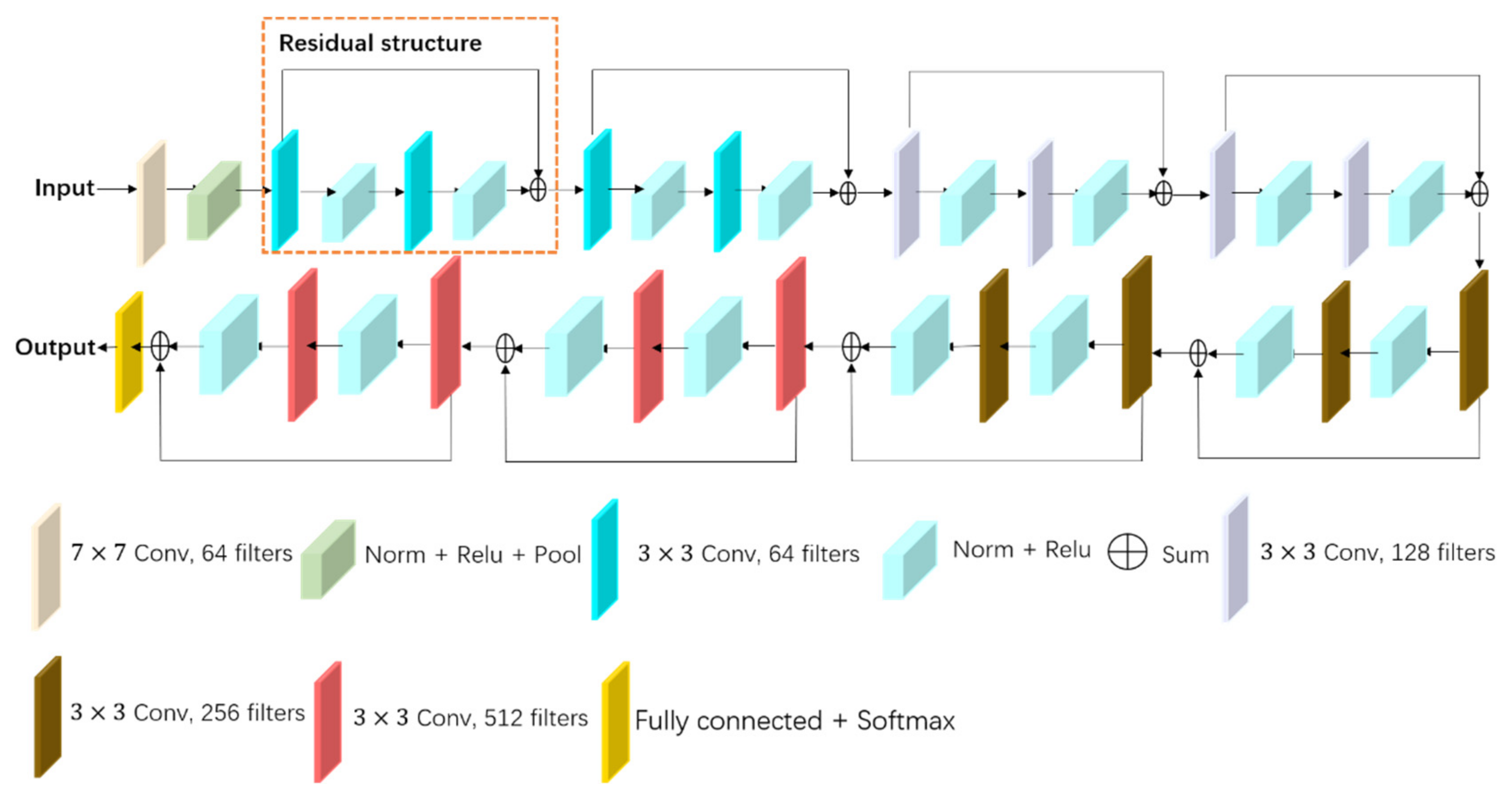
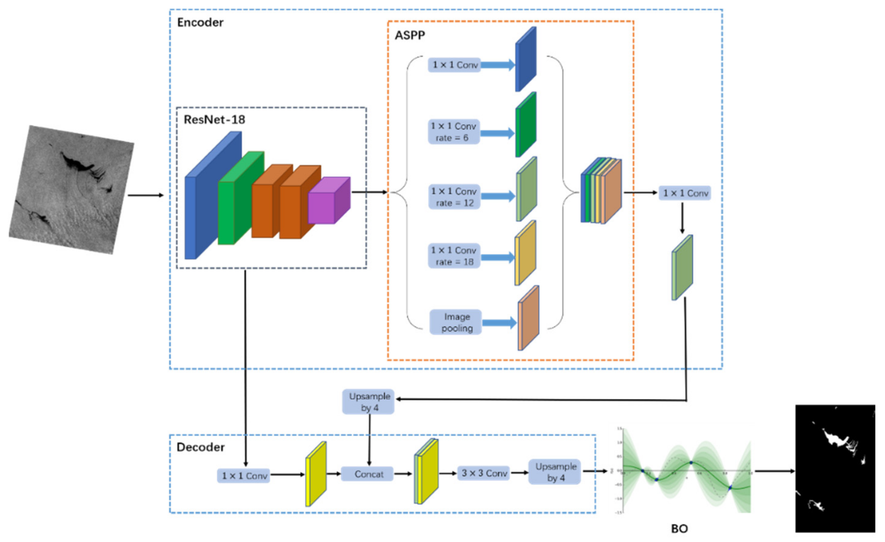
• ResNet-18, as the backbone in encoder of DeepLabv3+, can get more sufficiently feature extraction. ASPP (Atrous Spatial Pyramid Pooling) as an essential in encoder of DeepLabv3+, can expand the reception field to avoid loss of target information and get a fuller feature.
• Based on more sufficient and fuller feature extraction, BO was used to optimize hyperparameters and obtain optimal combinations of hyperparameters.

This paper is organized as follows: in Section 2, we describe the proposed BO-DRNet model based on BO, ResNet-18, and DeepLabv3+. Section 3 focuses on the preparation process of quad-polarimetric SAR images obtained by RADARSAT-2 and validates the oil spill detection capability for deep learning models. Section 4 contains a discussion. The conclusions are given in the final section.

2. The Proposed BO-DRNet Model

The traditional oil spill detection method usually consists of three main steps: (a) images segmentation technique detection of dark spots in the processed SAR image; (b) feature extraction from the initially identified regions; (c) classification as oil slick or non-oil slick regions. They have complicated steps and low detection accuracy. The proposed BO-DRNet is an end-to-end convolutional neural network for oil spill detection. It goes through downsampling layers for feature extraction from input based on encoder. To enhance the detection accuracy, BO optimizes the model’s hyperparameters. The model structure of BO-DRNet is shown in Figure 1.

2.1. Encoder

As shown in Figure 1, BO-DRNet’s encoder is composed of ResNet-18 and ASPP. ResNet-18 was proposed by He et al. in 2016 [40]. The model structure is shown in Figure 2. In ResNet-18, a very innovative residual structure was proposed. Residual structure explicitly fitted the residual mapping by convolution operation, rather than directly providing the desired based mapping by a stacked convolution operation. ResNet-18 changes the functional relationship to learning by the network layer into learning the residual function about the layer input. Therefore, it solves problems such as complex network convergence and gradient disappearance. Using the pretrained ResNet-18 as initialization can allow more sufficient feature extraction.

In addition, DeepLabv3+ as the most commonly used semantic segmentation model was proposed by Chen et al. in 2018 [41]. DeepLabv3+ introduces the encoder-decoder structure from the U-Net, which further fuses the underlying features with the high-level features to improve the segmentation accuracy. In the encoder of DeepLabv3+, the ASPP as a key was applied. ASPP can expand the reception field without changing the size of the feature map, which facilitates the extraction of multi-scale information. In BO-DRNet, the atrous rate of ASPP is 1,6,12, and 18. The output of ResNet-18 is the input for ASPP. The aim is that the extracted features are fully utilized while avoiding the loss of target information, and improving the detection accuracy.

2.2. Decoder

As shown in Figure 1, the decoder of BO-DRNet is DeepLabv3+’s decoder. It consists of convolution and deconvolution. The output of ResNet-18 passes through the 1 × 1 convolution kernel fed into decoder. The output feature depth concatenation with ASPP’s output, which uses four-fold deconvolution upsampling. The output feature fed into the 3 × 3 convolution kernel. The last output feature uses four-fold deconvolution upsampling. In the decoder, a skip connection is used to fuse the ResNet-18 extraction features and ASPP extraction features to recover input information. This fusion helps the model to recover fine object edges during upsampling. This is important for fine segmentation.

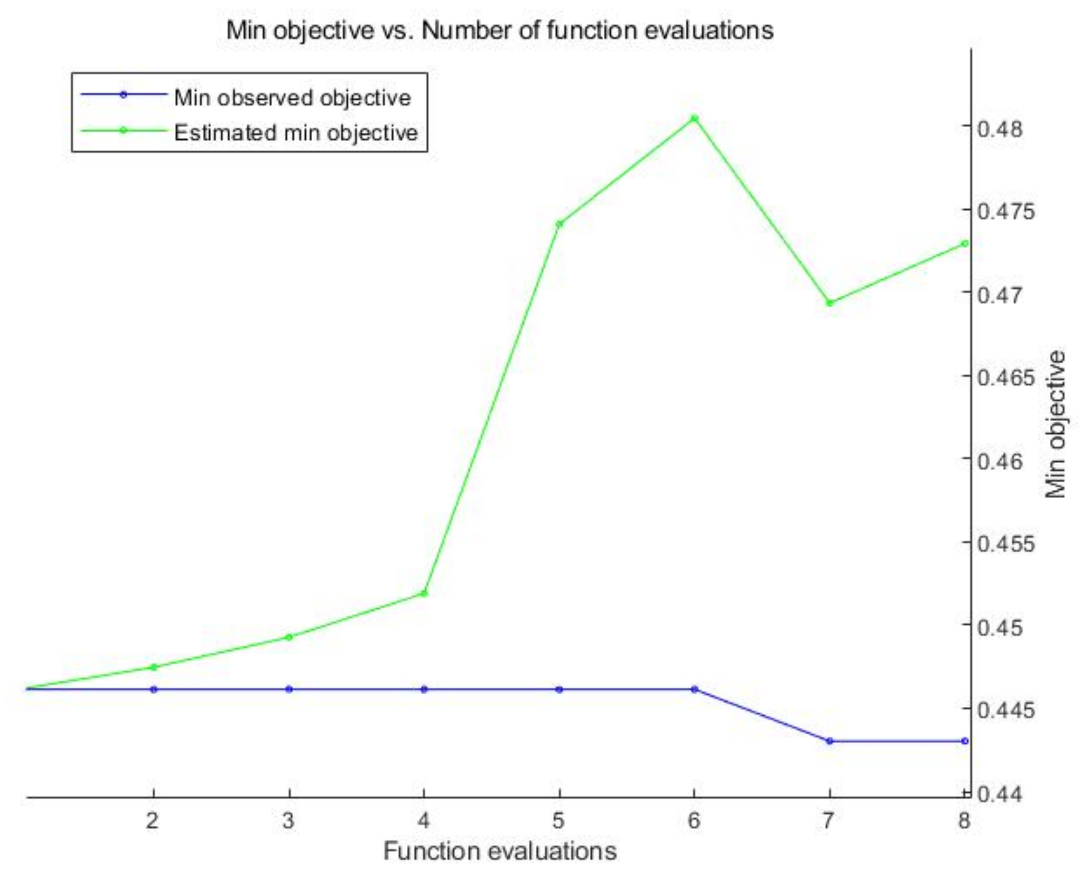
2.3. Bayesian Optimization (BO)

Bayesian Optimization (BO) was proposed by Frazier in 2018 [42]; the traditional and most commonly used method is Grid Search for hyperparameter optimization. It is unrealistic to experiment with the possible combination of hyperparameters. However, BO finds a better hyperparameter combination with minimal steps. It improves the efficiency and accuracy of hyperparameter optimization compared with traditional methods. Another advantage is that BO does not require a derivative, and the derivative of the hyperparameter is not available in general. These two advantages make BO the best method to adjust hyperparameters. The BO Algorithm 1 flow as shown below.

Algorithm 1: Bayesian Optimization (BO).

Input: f, X, S, M

D← InitSamplex (f, X)

for i←|D| to T do

p (y|x, D) ← FitModel (M, D)

xi ← argmaxx∈X S (x, p (y|x, D))

yi ← f(xi)

D←D ∪ (xi, yi)

end for

In the above Algorithm, f is the deep learning model, where an input of a set of hyperparameters get an output, X is the search space for the hyperparameters, and S is the acquisition function. In this study, oil spill pixels recognition accuracy is calculated, where D represents a dataset consisting of several pairs of data, each pair of arrays is represented as (x, y), x is a set of hyperparameters, y represents the result corresponding to the set of hyperparameters, M is the model obtained by fitting the dataset D, and T is the number of cycles. In this study, the goal is to find the x that minimizes S.

3. Dataset, Experiments, and Results

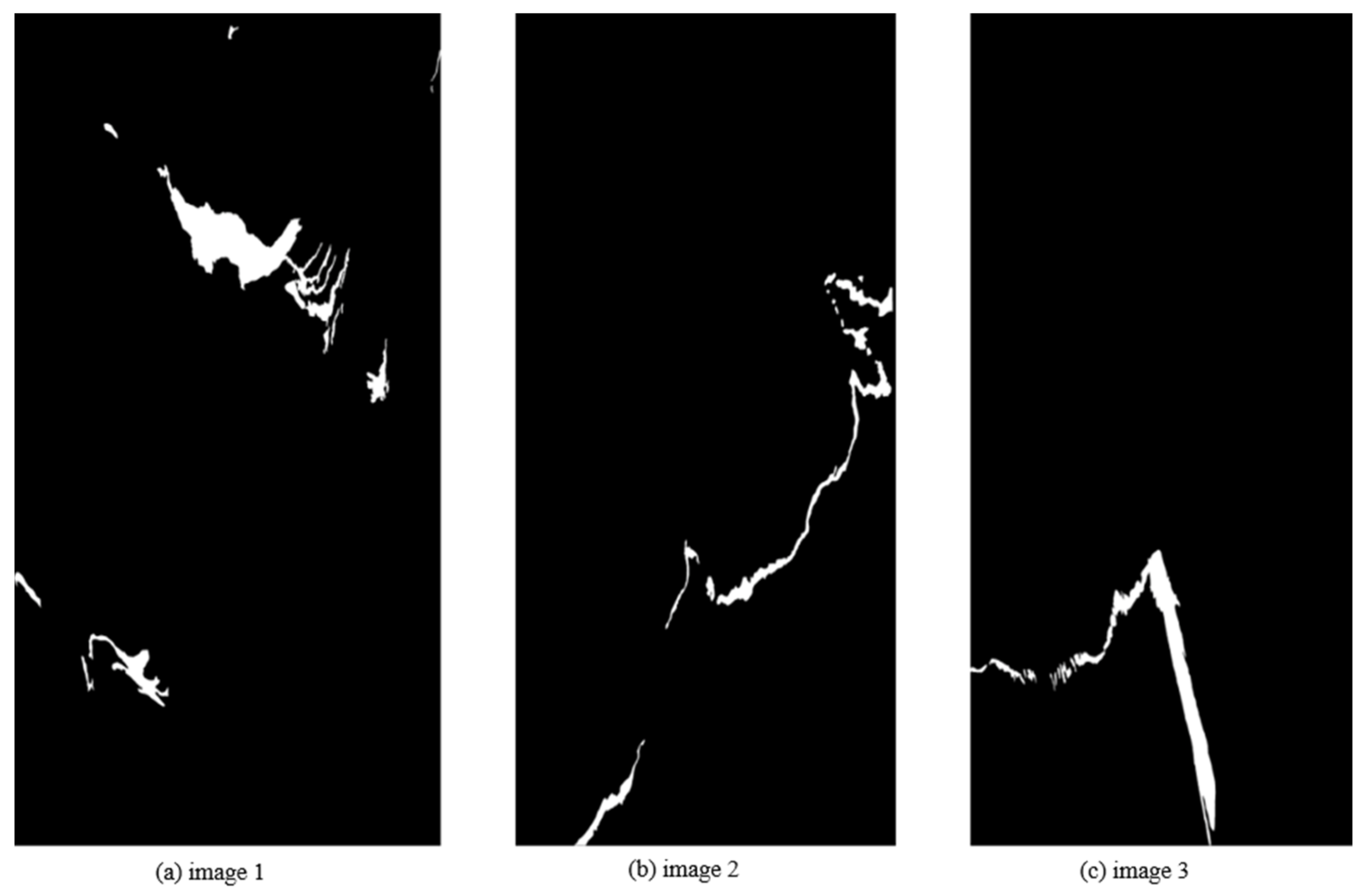
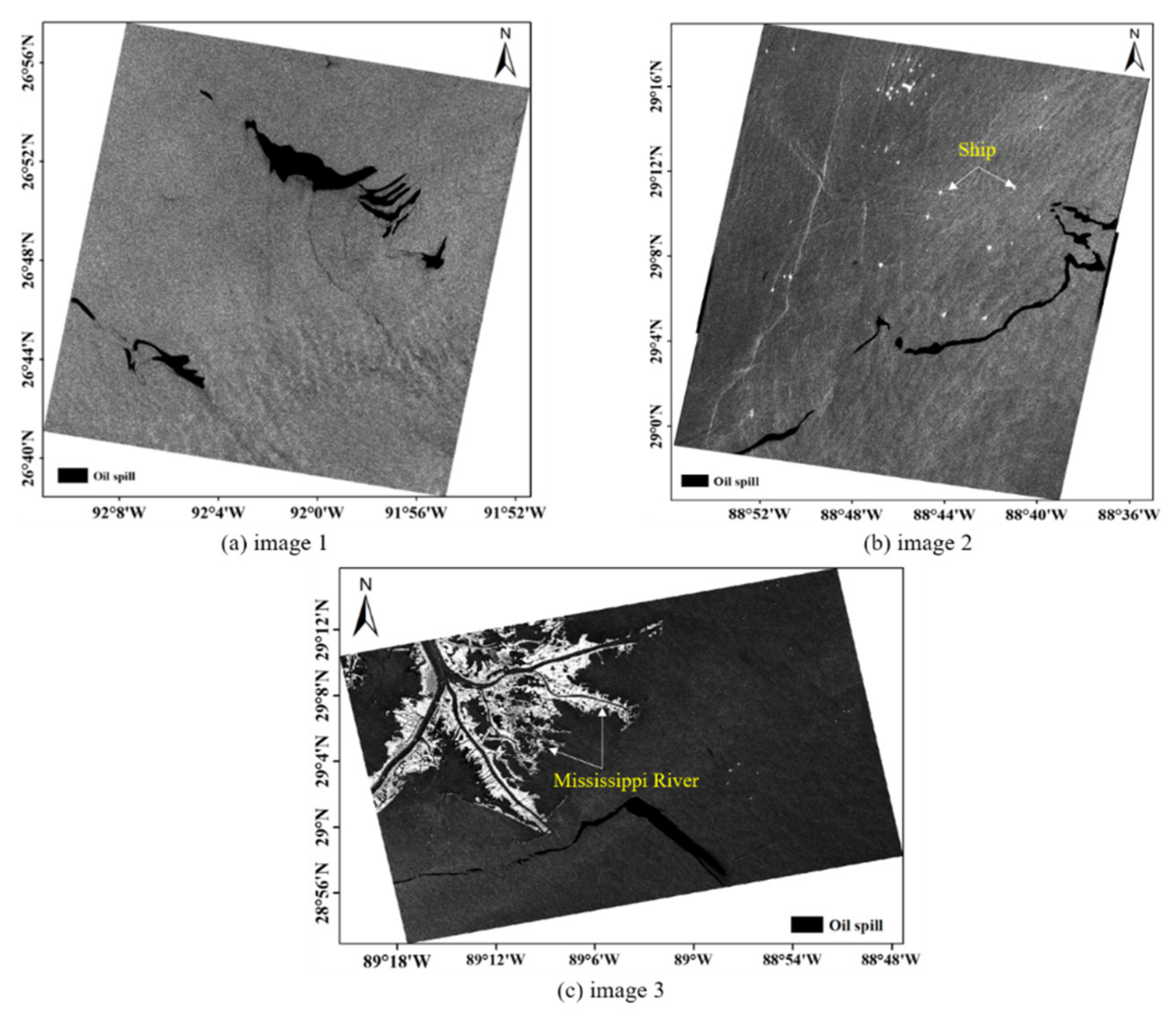
3.1. Oil Spill Dataset

In this paper, three quad-polarimetric oil spill SAR images were analyzed obtained by RADARSAT-2 over the Gulf of Mexico. The three images were acquired on 8 May 2010, 17 June 2011, and 8 May 2015. Detailed information of the three images is listed in

Table 1. Detailed information on the images used in this study, acquired by RADARSAT-2.

	Image 1	Image 2	Image 3
Time (UTC)	2010-05-08-12:01:25	2011-06-17-11:48:20	2015-05-08-23:53:36
Product type	SLC	SLC	SLC
Polarization	HH, VV, HV, VH	HH, VV, HV, VH	HH, VV, HV, VH
Beams	FQ23	Q25	Q8
Pixel spacing	4.73 m × 4.95 m	4.73 m × 5.05 m	4.73 m × 4.78 m
Size	6281 × 3920	7360 × 4089	6893 × 4904

.

Image 1 contains clear sea and oil spills, image 2 contains clear sea, ships, and oil spills, and image 3 contains clear sea, oil spills, and the Mississippi River. Figure 3 shows the three SAR images, including the location of oil spills, ships, and the Mississippi River.

3.2. Dataset Processing

For the three quad-polarimetric oil spill SAR images, ten prominent polarization features were used for oil spill detection, as shown in the introduction section. The quad-polarimetric SAR image can acquire a 2 × 2 complex scattering matrix S, as shown in Equation (1) as follows:

$$S=\left(\begin{array}{cc}{s}_{hh}& s_{hv}\\ s_{vh}& s_{vv}\end{array}\right)$$

(1)

where $v$ and $h$ represent the scattering amplitude. Based on the reciprocity theorem, $s_{hv}=s_{vh}$. In addition, the scattering matrix can vectorize as $k_1={\left[s_{hv}\sqrt{2}{s}_{hv}{s}_{vv}\right]}^T$, where T denotes the matrix transpose. The covariance matrix can be obtained by Equation (2):

$$C=k_1{k}_1{}^{\ast T}=\left[\begin{array}{l}{\left|s_{hh}\right|}^2\sqrt{2}{s}_{hh}{s}_{hv}^{\ast }{s}_{hh}{s}_{vv}^{\ast }\\ \sqrt{2}{s}_{hv}{s}_{hh}^{\ast }2{\left|s_{hh}\right|}^2\sqrt{2}{s}_{hv}{s}_{vv}^{\ast }\\ s_{vv}{s}_{hh}^{\ast }\sqrt{2}{s}_{vv}{s}_{hv}^{\ast }{\left|s_{vv}\right|}^2\end{array}\right]$$

(2)

where $\ast T$ denotes conjugate transpose. Moreover, the scattering matrix can also vectorize as $k_2=\frac{1}{\sqrt{2}}{\left[s_{hh}+s_{vv}{s}_{hh}-s_{vv}2s_{hv}\right]}^T$, while the coherency matrix can be obtained by Equation (3):

$$T=k_2{k}_2{}^{\ast T}=\frac{1}{2}\left[\begin{array}{l}\left(s_{hh}+s_{vv}\right)\left(s_{hh}+s_{vv}\right){}^{\ast }\left(s_{hh}+s_{vv}\right)\left(s_{hh}-s_{vv}\right){}^{\ast }2\left(s_{hh}+s_{vv}\right)s_{hv}^{\ast }\\ \left(s_{hh}-s_{vv}\right)\left(s_{hh}+s_{vv}\right){}^{\ast }\left(s_{hh}-s_{vv}\right)\left(s_{hh}-s_{vv}\right){}^{\ast }2\left(s_{hh}-s_{vv}\right)s_{hv}^{\ast }\\ 2s_{hv}\left(s_{hh}+s_{vv}\right){}^{\ast }2s_{hv}\left(s_{hh}-s_{vv}\right){}^{\ast }4s_{hv}{s}_{hv}^{\ast }\end{array}\right]$$

(3)

The covariance matrix and the correlation matrix are Ermitian semi-positive definite matrices with the same eigenvalues and can be transformed into each other. Equations (4) and (5) are as follows:

$$T=AC{A}^T$$

(4)

$$A=\frac{1}{\sqrt{2}}\left[\begin{array}{l}101\\ 10-1\\ 0\sqrt{2}0\end{array}\right]$$

(5)

Based on the above calculation principles, first, PolSARpro software (v6.0, a tool for self-education in the field of Polarimetric SAR data analysis) is used to get the coherency matrix. Each pixel for the dataset can get a coherency matrix. Then, PolSARpro software is used to gain total power of the SAR scattering target, entropy, conformity coefficient, degree of polarization, mean scattering angle, and anisotropy.

The total power of the SAR scattering target can be obtained by Equation (6) as follows:

$$span={\left|s_{hh}\right|}^2+2{\left|s_{hv}\right|}^2+{\left|s_{vv}\right|}^2$$

(6)

The entropy, Equations (7) and (8), is calculated as follows:

$$H=-{\displaystyle \sum _{i=1}^3{p}_i}{\log }_3{p}_i$$

(7)

$$p_i=\frac{{\lambda }_3}{{\displaystyle \sum _{i=1}^3{\lambda }_i}}$$

(8)

where ${\lambda }_i$ is the weight of corresponding scattering mechanisms. The anisotropy, Equation (9), is calculated as follows:

$$A=\frac{{\lambda }_2-{\lambda }_3}{{\lambda }_2+{\lambda }_3},\left({\lambda }_2>{\lambda }_3\right)$$

(9)

where ${\lambda }_i$ is the same as in Equation (8). The conformity coefficient, Equation (10), is calculated as follows:

$$\mu \cong \frac{2\left(\Re \left(S_{hh}{S}_{vv}^{*}\right)-{\left|S_{hv}\right|}^2\right)}{\left({\left|S_{hh}\right|}^2+2{\left|S_{hv}\right|}^2+{\left|S_{vv}\right|}^2\right)}$$

(10)

where $\Re$ is a real part of scattering matrix. The degree of polarization, Equation (11), is calculated as follows:

$$DoP=\frac{\sqrt{S^s\left(2\right)+S^s\left(3\right)+S^s\left(4\right)}}{S^s\left(1\right)}$$

(11)

where $S^s\left(i\right)$ is an element of scattered Stokes vector. The mean scattering angle Equation (12) is calculated as follows:

$$\alpha ={\displaystyle \sum _{i=1}^3{p}_i{\alpha }_i}$$

(12)

where ${\alpha }_i$ is a phase related to each scattering mechanisms.

Lastly, we use MATLAB (2020B) to get the geometric intensity, muller matrix, co-polarized phase difference, and co-polarized complex correlation based on the coherency matrix. The geometric intensity, Equation (13), is calculated as follows:

$$\upsilon =\det {\left(T\right)}^{\frac{1}{d}}$$

(13)

where d is the dimension of the covariance matrix. In the dual-polarization SAR image, d is 2, while d is 3 in the quad-polarization SAR image. The muller matrix, Equation (14), is calculated as follows:

$$M_{33}=〈\Re \left(S_{hh}{S}_{vv}^{*}+{\left|S_{hv}\right|}^2\right)〉$$

(14)

The co-polarized phase difference Equation (15) is calculated as follows:

$${\sigma }_{\varphi CO}=\angle \left(S_{hh}{S}_{vv}^{*}\right)$$

(15)

where $\angle$ is the mean phase. The co-polarized complex correlation, Equation (16), is calculated as follows:

$$\rho =\left|\frac{〈S_{hh}{S}_{vv}^{*}〉}{\sqrt{〈{\left|S_{hh}\right|}^2〉〈{\left|S_{vv}\right|}^2〉}}\right|$$

(16)

The ten prominent polarization features extracted from image 1, image 2, and image 3 compose dataset 1, dataset 2, and dataset 3, respectively. In addition, since different polarization features take different ranges of values, they are normalized by MATLAB to increase their comparability. Ten prominent polarization features of the three SAR images are shown in Figure 4, Figure 5 and Figure 6. The oil spill area is relatively evident by observing the three images, which plays a positive role in oil spill detection.

3.3. Experiment

As shown in Figure 3, there are other classes besides oil spills in the three SAR images. This paper focuses on oil spill detection; hence, there are only oil spill pixels and non-oil spill pixels in the SAR images. Thus, first, in combination with relevant a priori knowledge, the oil spill pixels were marked manually for the three SAR images. The binary images are shown in Figure 7. In this figure, white represents oil spill pixels, while black represents non-oil spill pixels.

The number of oil spill pixels for each dataset as shown in

Table 2. The number of oil spill pixels for each dataset used in this study.

	Dataset 1	Dataset 2	Dataset 3
Number of oil spill pixels	634,916	421,332	609,964

.

Then, since the BO-DRNet model requires the input is 256 × 256 × n, n represents the number of features. Thus, 32,768 oil spill pixels and 32,768 non-oil spill pixels are randomly selected as the training set and the other pixels as the test set for each dataset. To evaluate the recognition ability of the proposed model, FCN-8s, DeepLabv3+Xception, and DeepLabv3+ResNet-18 were used in this experiment. FCN-8s is an end-to-end convolution neural network. Unlike the classical CNN (Convolutional Neural Network), which uses a fully connected layer to obtain a fixed-length feature vector for classification, FCN-8s replace the fully connected layer with a convolutional layer that can accept an input image with an arbitrary size that uses a deconvolutional layer to upsample. The feature map is used to restore the output image to the same size of the input image. This can produce a prediction for each pixel while preserving the original input spatial information of the image. Finally, a feature map is used for pixel classification. All experiments were done in the MATLAB (2020B) software platform.

Accuracy and dice are used to measure the oil spill detection ability of a deep learning model. Dice is a similarity measurement function, usually used as an evaluation index for semantic segmentation to calculate the similarity of two samples. The value range is 0 to 1. Equations (17)–(19) are as follows:

$$Accuracy=\frac{TP}{TP+FN}$$

(17)

$$Dice=\frac{2\times Jaccard}{1+Jaccard}$$

(18)

$$Jaccard=\frac{Predict\cap Ture}{Predict\cup Ture}$$

(19)

From the above Equations, TP defines the pixel number of true positive, and FN defines the pixel number of false negative. Predict is the predict label of dataset, while True is the true label of dataset. The closer the value of accuracy and dice is to 1, the better the recognition ability of the model.

3.4. Results

3.4.1. Results of BO

In deep learning models, the primary hyperparameters include the initial learning rate, stochastic gradient descent momentum, and L2 regularization strength, which are optimized by BO. The relevant descriptions and value range of hyperparameters are shown in

Table 3. The descriptions, value ranges, and the optimal value of hyperparameters by BO used in this study.

Hyper-Parameter	Description	Value Ranges	The Optimal Value
Initial learning rate	The best learning rate depend on your data when the network is training.	$[{10}^{-2},1]$	0.1235
Stochastic gradient descent momentum	Momentum adds inertia to the parameter updates by having the current update contain a contribution proportional to the update in the previous iteration.	$\left[0.8,0.98\right]$	0.8018
L2 regularization strength	Use regularization to prevent overfitting. Search the space of regularization strength to find a good value.	$\left[{10}^{-10},{10}^{-2}\right]$	$1.102\times {10}^{-10}$

. The optimization process is shown in Figure 8. Combining the min observed objective and estimated min objective, the seventh function evaluation is the optimal result for the hyperparameters. The optimal value of these hyperparameters as shown in Table 3. By BO, the initial learning rate is 0.1235, the stochastic gradient descent momentum is 0.81018, and the L2 regularization strength is 1.102 × 10⁻¹⁰.

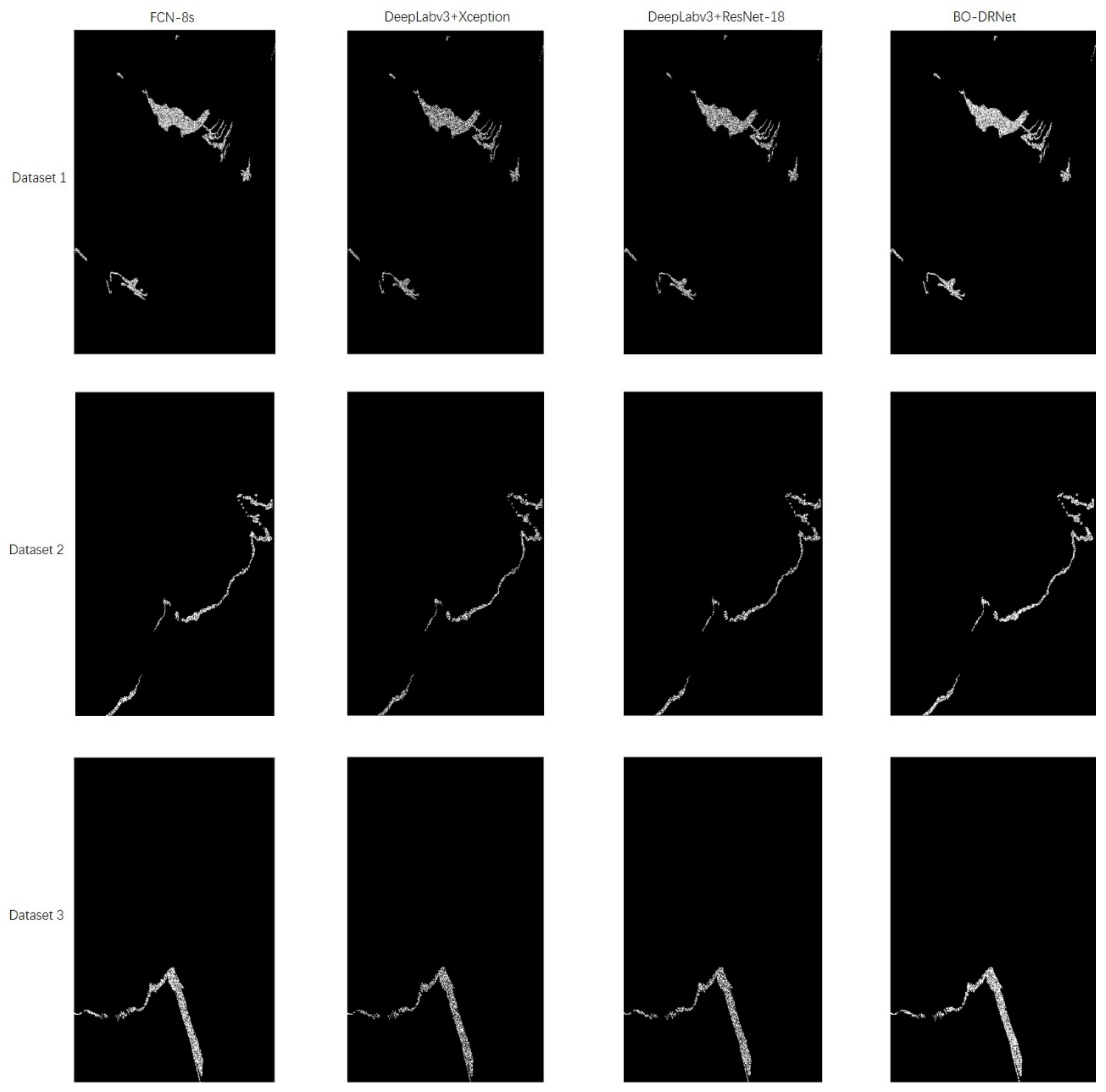
3.4.2. Results of Deep Learning Models

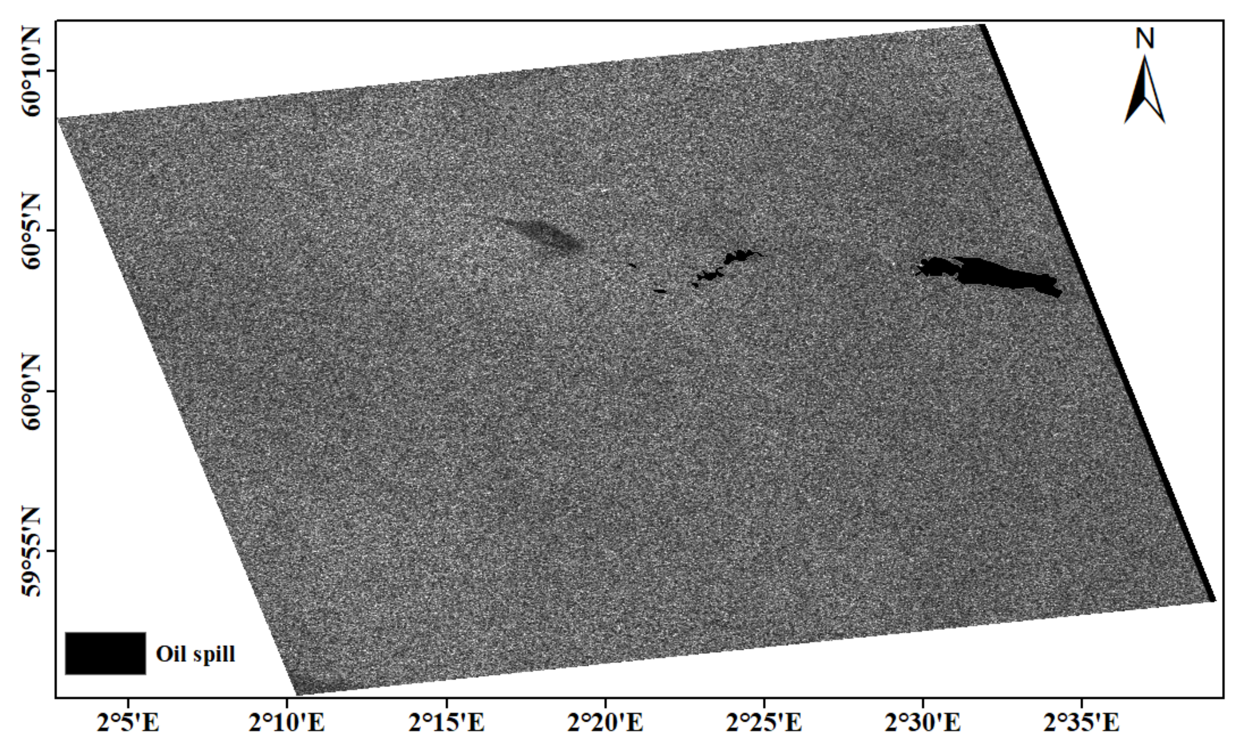
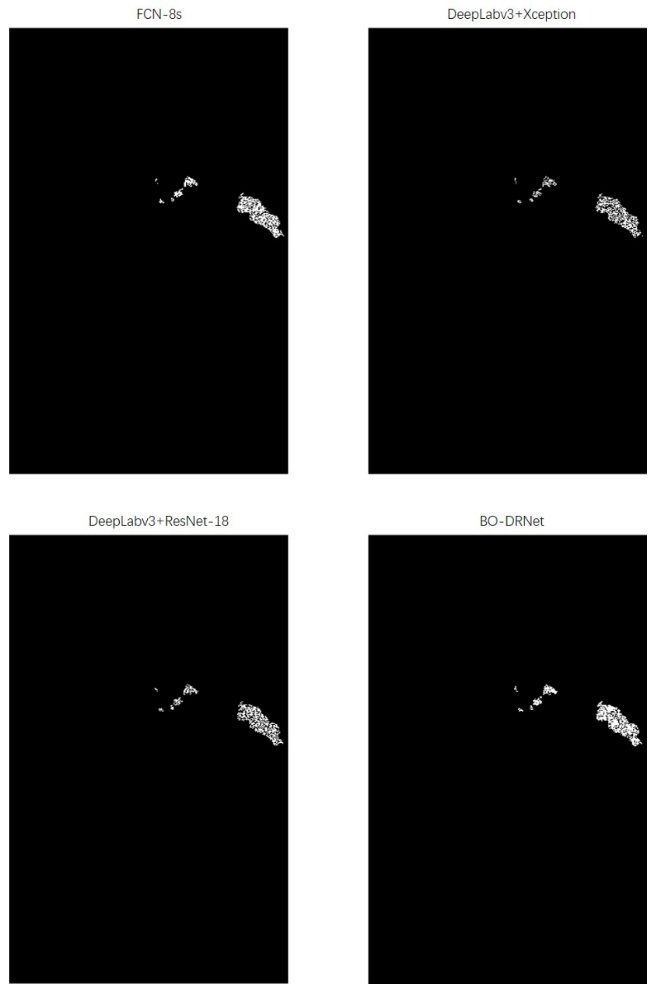
To better reflect the differences between different deep learning models, the fixed hyperparameters were used to train and test FCN-8s, DeepLabv3+Xception, and DeepLabv3+ResNet-18. Detailed information on the hyperparameters is shown in

Table 4. Fixed hyperparameters and values for FCN-8s, DeepLabv3+Xception, and DeepLabv3+ResNet-18.

Hyperparameters	Value
Patches Per Image	1600
Initial learning rate	0.05
Stochastic gradient descent momentum	0.90
Epoch	10
Mini batch size	16
L2 regularization strength	${10}^{-4}$

. For BO-DRNet, except for the hyperparameters by BO, the values are the same as in Table 4.

The results are listed in

Table 5. The experimental results of four deep learning models for three datasets.

	Model	FCN-8s	DeepLabv3+Xception	DeepLabv3+Resnet18	BO-DRNet
Accuracy (%)	Dataset 1	70.16	54.31	59.93	75.06
	Dataset 2	70.19	56.92	60.81	74.64
	Dataset 3	69.89	55.03	59.48	74.38
Mean accuracy (%)		70.08	55.42	60.07	74.69
dice	Dataset 1	0.8247	0.7039	0.7494	0.8575
	Dataset 2	0.8248	0.7254	0.7563	0.8548
	Dataset 3	0.8228	0.7099	0.7459	0.8531
Mean dice		0.8241	0.7131	0.7505	0.8551

. From this table, we can observe that each model has a similar recognition accuracy for each dataset. BO-DRNet accurately identifies oil spill pixels with the highest mean accuracy of 74.69% and the best mean dice of 0.8551. The improved model improves recognition accuracy by 4.61% over the second and 19.27% over the last. In addition, compared with DeepLabv3+ResNet-18, the recognition accuracy of BO-DRNet was enhanced by 14.62%, and the dice improved by 0.1046. Therefore, BO is vital for the recognition ability of deep learning models.

The binary images are made according to the model recognition results, as shown in Figure 9.

3.5. Validation

In this section, another quad-polarimetric oil spill SAR image obtained by RADARSAT-2 was used to validate the proposed model recognition capability for oil spill pixels. This image is from the NOFO (Norwegian Clean Seas Association for Operating Companies). The NOFO conducted an oil-on-water exercise in Norwegian waters in June 2011. Detailed information of the image is listed in

Table 6. Details information on the image acquisition by RADARSAT-2 used in this study.

	SAR Image
Time (UTC)	2011-06-08-17:27:53
Product type	SLC
Polarization	HH, VV, HV, VH
Beams	Q15
Pixel spacing	4.73 m × 4.82 m
Size	7120 × 3369

.

In this exercise, oil emulsion and crude oil are on the sea surface. Figure 10 shows the SAR image and the location of the oil spill.

The dataset is processed by PolSARpro software and MATLAB, the ten prominent polarization features are obtained, and dataset 4 is composed. MATLAB also normalized this dataset to increase the comparability between different polarization features. Meanwhile, with relevant a priori knowledge, oil spill pixels were marked manually for the SAR image, and the binary image is shown in Figure 11. White represents oil spill pixels, while black represents non-oil spill pixels in this figure.

Finally, we used FCN-8s, DeepLabv3+Xception, DeepLabv3+ResNet-18, and BO-DRNet trained on dataset 1, dataset 2, and dataset 3 to identify oil spill pixels for dataset 4. Accuracy and dice are used to measure the detection ability of deep learning models.

Table 7. The experimental results of four deep learning models for dataset 4.

Model	FCN-8s	DeepLabv3+Xception	DeepLabv3+resnet18	BO-DRNet
Accuracy (%)	69.95	57.48	58.55	75.03
Dice	0.8232	0.7300	0.7386	0.8573

presents the experimental results of four deep learning models for dataset 4. It shows that the BO-DRNet has the best recognition accuracy, i.e., 0.7503, while the dice is 0.8573. This demonstrates the general solid adaptability and robustness of the proposed model.

The binary images made according to the model recognition results are shown in Figure 12.

4. Discussion

4.1. Impact of the Training Set Number

To get better feature extraction and expand the reception field, we used ResNet-18 and SAPP as the backbone of the encoder of the proposed deep learning model—BO-DRNet. In addition, BO was used to optimize and obtain the optimal combination of BO-DRNet’s hyperparameters. Compared with the three other deep learning models, BO-DRNet achieved high accuracy in the experiment. However, many oil spill pixels have not been detected correctly, as shown in Figure 9 and Figure 12. We believe that the reason for this result may be the number of training sets. The number of training sets is about 5% of the total oil spill pixels in each dataset. A deep learning model usually requires big data to extract useful features to improve classification performance [43]. For example, Shaban et al. used 80% of the dataset to train a novel convolutional neural network framework and minimize the generalized dice loss [36]. In the following study, we will increase the number of randomly selected training sets to improve the recognition accuracy of deep learning models.

4.2. Impact of the Hyperparameter

In this study, the BO-DRNet significantly improved the recognition accuracy compared to other models. Therefore, hyperparameters have a very substantial influence on results. Claesen et al. suggested that hyperparameters can be used to configure various aspects of the learning algorithm and can significantly affect the resulting model and its performance [44]. However, Hyperparameter Optimization is commonly performed manually, via rules-of-thumb or testing some hyperparameter combinations. These methods are impractical when the number of hyperparameters is large. Therefore, optimization is receiving an increasing amount of attention in deep learning. In the following study, we will further improve the hyperparameter optimization method to enhance the identification ability of the model.

4.3. Future Study

First, this paper demonstrates the possibility of using a deep learning model-based polarization feature for oil spill detection, since the polarization feature can provide feature information that can positively affect oil spill detection. We will carefully discuss and research a more effective polarization feature selection method to enhance oil spill detection accuracy in the future. Moreover, the complex marine environment is a massive challenge for oil spill detection; there are ships, drilling rigs, and look-alikes oil spills. In the future, we will further improve the deep learning model and extract more useful abstract features to enhance the classification accuracy in the complex marine environment.

Second, the true oil spill pixels are manually marked in this study. This method consumes a lot of time and inevitably has errors. However, unsupervised feature learning can learn feature representations with supervision and has been successfully applied to recognizing remote scenes and targets [45]. Therefore, in a future study, we will use an unsupervised approach, such as the Self-Organizing Map (SOM) and hierarchical clustering, to mark the dataset and provide superior performance.

5. Conclusions

This paper proposes an improved deep learning model for oil spill detection based on polarimetric features from quad-polarimetric oil spill SAR images obtained by RADARSAT-2. The model is named BO-DRNet. It contains ResNet-18 as the backbone of the encoder of DeepLabv3+, and BO was used to optimize its hyperparameters. In BO-DRNet, ResNet-18 can get a more sufficient feature extraction, while ASPP can expand the reception field. Ten prominent polarimetric features were extracted and composed the dataset for each SAR image. Three datasets were used to train and test the model. Besides FCN-8s, DeepLabv3+Xception and DeepLabv3+ResNet-18 were used for this experiment under the same conditions. Accuracy and dice were used to evaluate the model recognition capability. The experimental results show that the BO-DRNet gets a better recognition ability for oil spill pixels than the other three models. In addition, another quad-polarimetric oil spill SAR image obtained by RADARSAT-2 was used to validate the improved model in the same conditions and achieved the highest recognition accuracy. This proves that the proposed model has a strong general adaptability and robustness. The improved model provides a new research idea for future marine oil spill detection.

References

1. Kvenvolden, K.A.; Cooper, C.K. Natural seepage of crude oil into the marine environment. Geo-Mar. Lett. 2003, 23, 140–146. [Google Scholar] [CrossRef]
2. Jiao, Z.; Jia, G.; Cai, Y. A new approach to oil spill detection that combines deep learning with unmanned aerial vehicles. Comput. Ind. Eng. 2019, 135, 1300–1311. [Google Scholar] [CrossRef]
3. Liu, Y.; MacFadyen, A.; Ji, Z.G.; Weisberg, R.H. (Eds.) Monitoring and Modeling the Deepwater Horizon Oil Spill: A Recordbreaking Enterprise; American Geophysical Union, Geopress: Washington, DC, USA, 2011; Volume 195, p. 271. [Google Scholar]
4. White, H.K.; Hsing, P.Y.; Cho, W.; Shank, T.M.; Cordes, E.E.; Quattrini, A.M.; Nelson, R.K.; Camilli, R.; Demopoulos, A.W.J.; German, C.R.; et al. Impact of the Deepwater Horizon oil spill on a deep-water coral community in the Gulf of Mexico. Proc. Natl. Acad. Sci. USA 2012, 109, 20303–20308. [Google Scholar] [CrossRef] [Green Version]
5. Keramitsoglou, I.; Cartalis, C.; Kiranoudis, C.T. Automatic identification of oil spills on satellite images. Environ. Model. Softw. 2006, 21, 640–652. [Google Scholar] [CrossRef]
6. Skrunes, S.; Brekke, C.; Eltoft, T. Characterization of marine surface slicks by Radarsat-2 multipolarization features. IEEE Trans. Geosci. Remote Sens. 2013, 52, 5302–5319. [Google Scholar] [CrossRef] [Green Version]
7. Zheng, H.; Zhang, Y.; Wang, Y.; Zhang, X.; Meng, J. The polarimetric features of oil spills in full polarimetric synthetic aperture radar images. Acta Oceanol. Sin. 2017, 36, 105–114. [Google Scholar] [CrossRef]
8. Zeng, K.; Wang, Y. A deep convolutional neural network for oil spill detection from spaceborne SAR images. Remote Sens. 2020, 12, 1015. [Google Scholar] [CrossRef] [Green Version]
9. Zhang, B.; Perrie, W.; Li, X.; Pichel, W.G. Mapping sea surface oil slicks using RADARSAT-2 quad-polarization SAR image. Geophys. Res. Lett. 2011, 38. [Google Scholar] [CrossRef] [Green Version]
10. Zheng, H.; Zhang, Y.; Wang, Y. Polarimetric features analysis of oil spills in C-band and L-band SAR images. In Proceedings of the International Geoscience and Remote Sensing Symposium, IGARSS 2016, Beijing, China, 11–15 July 2016; pp. 4683–4686. [Google Scholar]
11. Migliaccio, M.; Nunziata, F.; Buono, A. SAR polarimetry for sea oil slick observation. Int. J. Remote Sens. 2015, 36, 3243–3273. [Google Scholar] [CrossRef] [Green Version]
12. Nunziata, F.; Migliaccio, M.; Li, X. Sea oil slick observation using hybrid-polarity SAR architecture. IEEE J. Ocean. Eng. 2014, 40, 426–440. [Google Scholar] [CrossRef]
13. Migliaccio, M.; Gambardella, A.; Tranfaglia, M. SAR polarimetry to observe oil spills. IEEE Trans. Geosci. Remote Sens. 2007, 45, 506–511. [Google Scholar] [CrossRef]
14. Migliaccio, M.; Nunziata, F.; Gambardella, A. On the co-polarized phase difference for oil spill observation. Int. J. Remote Sens. 2009, 30, 1587–1602. [Google Scholar] [CrossRef]
15. Skrunes, S.; Brekke, C.; Eltoft, T. Oil spill characterization with multi-polarization C-and X-band SAR. In Proceedings of the International Geoscience and Remote Sensing Symposium, IGARSS 2012, Munich, Germany, 22–27 July 2012; pp. 5117–5120. [Google Scholar]
16. Bing, D.; Jinsong, C. An algorithm based on cross-polarization ratio of SAR image for discriminating between mineral oil and biogenic oil. Remote Sens. Technol. Appl. 2013, 28, 103–107. [Google Scholar]
17. Yin, J.; Moon, W.; Yang, J. Model-based pseudo-quad-pol reconstruction from compact polarimetry and its application to oil-spill observation. J. Sens. 2015, 2015. [Google Scholar] [CrossRef]
18. Shirvany, R.; Chabert, M.; Tourneret, J.Y. Ship and oil-spill detection using the degree of polarization in linear and hybrid/compact dual-pol SAR. IEEE J. Sel. Top. Appl. Earth Observ. 2012, 5, 885–892. [Google Scholar] [CrossRef] [Green Version]
19. Migliaccio, M.; Nunziata, F.; Montuori, A.; Li, X.; Pichel, W.G. A multifrequency polarimetric SAR processing chain to observe oil fields in the Gulf of Mexico. IEEE Trans. Geosci. Remote Sens. 2011, 49, 4729–4737. [Google Scholar] [CrossRef]
20. Song, D.; Wang, B.; Chen, W.; Wang, N.; Yu, S.; Ding, Y.; Liu, B.; Zhen, Z.; Xu, M.; Zhang, T. An efficient marine oil spillage identification scheme based on an improved active contour model using fully polarimetric SAR imagery. IEEE Access 2018, 6, 67959–67981. [Google Scholar] [CrossRef]
21. Garcia-Pineda, O.; Zimmer, B.; Howard, M.; Pichel, W.; Li, X.; MacDonald, I.R. Using SAR images to delineate ocean oil slicks with a texture-classifying neural network algorithm (TCNNA). Can. J. Remote Sens. 2009, 35, 411–421. [Google Scholar] [CrossRef]
22. Solberg, A.H.S.; Solberg, R. A large-scale evaluation of features for automatic detection of oil spills in ERS SAR image. In Proceedings of the International Geoscience and Remote Sensing Symposium, IGARSS 1996, Lincoln, NE, USA, 2–31 May 1996; pp. 1484–1486. [Google Scholar]
23. Topouzelis, K.; Psyllosm, A. Oil spill feature selection and classification using decision tree forest on SAR image data. ISPRS J. Photogramm. Remote Sens. 2012, 68, 135–143. [Google Scholar] [CrossRef]
24. Singha, S.; Vespe, M.; Trieschmann, O. Automatic Synthetic Aperture Radar based oil spill detection and performance estimation via a semi-automatic operational service benchmark. Mar. Pollut. Bull. 2013, 73, 199–209. [Google Scholar] [CrossRef]
25. Topouzelis, K.; Karathanassi, V.; Pavlakis, P.; Rokos, D. Detection and discrimination between oil spills and look-alike phenomena through neural networks. ISPRS J. Photogramm. Remote Sens. 2007, 62, 264–270. [Google Scholar] [CrossRef]
26. Del Frate, F.; Petrocchi, A.; Lichtenegger, J.; Calabresi, G. Neural networks for oil spill detection using ERS-SAR data. IEEE Trans. Geosci. Remote Sens. 2000, 38, 2282–2287. [Google Scholar] [CrossRef] [Green Version]
27. Singha, S.; Bellerby, T.J.; Trieschmann, O. Satellite oil spill detection using artificial neural networks. IEEE J. Sel. Top. Appl. Earth Obs. Remote Sens. 2013, 6, 2355–2363. [Google Scholar] [CrossRef]
28. Brekke, C.; Solberg, A.H.S. Classifiers and confidence estimation for oil spill detection in ENVISAT ASAR images. IEEE Geosci. Remote Sens. Lett. 2008, 5, 65–69. [Google Scholar] [CrossRef]
29. Xu, L.; Li, J.; Brenning, A. A comparative study of different classification techniques for marine oil spill identification using RADARSAT-1 imagery. Remote Sens. Environ. 2014, 141, 14–23. [Google Scholar] [CrossRef]
30. Singha, S.; Ressel, R.; Velotto, D.; Lehner, S. A combination of traditional and polarimetric features for oil spill detection using TerraSAR-X. IEEE J. Sel. Top. Appl. Earth Obs. Remote Sens. 2016, 9, 4979–4990. [Google Scholar] [CrossRef] [Green Version]
31. Solberg, A.H.S.; Volden, E. Incorporation of prior knowledge in automatic classification of oil spills in ERS SAR images. In Proceedings of the International Geoscience and Remote Sensing Symposium, IGARSS 1997, Singapore, 3–8 August 1997; pp. 157–159. [Google Scholar]
32. Solberg, A.H.S.; Storvik, G.; Solberg, R.; Volden, E. Automatic detection of oil spills in ERS SAR images. IEEE Trans. Geosci. Remote Sens. 1999, 37, 1916–1924. [Google Scholar] [CrossRef] [Green Version]
33. Huang, X.; Wang, X. The classification of synthetic aperture radar oil spill images based on the texture features and deep belief network. In Computer Engineering and Networking; Springer: Cham, Switzerland, 2014; pp. 661–669. [Google Scholar]
34. Chen, G.; Li, Y.; Sun, G.; Zhang, Y. Application of deep networks to oil spill detection using polarimetric synthetic aperture radar images. Appl. Sci. 2017, 7, 968. [Google Scholar] [CrossRef]
35. Gallego, A.J.; Gil, P.; Pertusa, A.; Fisher, R. Segmentation of oil spills on side-looking airborne radar imagery with autoencoders. Sensors 2018, 18, 797. [Google Scholar] [CrossRef] [Green Version]
36. Shaban, M.; Salim, R.; Abu Khalifeh, H.; Khelifi, A.; Shalaby, A.; EI-Mashad, S.; Mahmoud, A.; Ghazal, M.; EI-Baz, A. A Deep-Learning Framework for the Detection of Oil Spills from SAR Data. Sensors 2021, 21, 2351. [Google Scholar] [CrossRef]
37. Ma, X.; Xu, J.; Wu, P.; Kong, P. Oil Spill Detection Based on Deep Convolutional Neural Networks using Polarimetric Scattering Information from Sentinel-1 SAR Images. IEEE Trans. Geosci. Remote Sens. 2021. [Google Scholar] [CrossRef]
38. Krestenitis, M.; Orfanidis, G.; Ioannidis, K.; Avgerinakis, k.; Vrochidis, S.; Kompatsiaris, I. Oil spill identification from satellite images using deep neural networks. Remote Sens. 2019, 11, 1762. [Google Scholar] [CrossRef] [Green Version]
39. Guo, H.; Wu, D.; An, J. Discrimination of oil slicks and lookalikes in polarimetric SAR images using CNN. Sensors 2017, 17, 1837. [Google Scholar] [CrossRef] [Green Version]
40. He, K.; Zhang, X.; Ren, S.; Sun, J. Deep residual learning for image recognition. In Proceedings of the IEEE Conference on Computer Vision and Pattern Recognition, CVPR 2016, Las Vegas, NV, USA, 27–30 June 2016; pp. 770–778. [Google Scholar]
41. Chen, L.C.; Zhu, Y.; Papandreou, G.; Schroff, F.; Adam, H. Encoder-decoder with atrous separable convolution for semantic image segmentation. In Proceedings of the European Conference on Computer Vision, ECCV 2018, Munich, Germany, 8–14 September 2018; pp. 801–818. [Google Scholar]
42. Frazier, P.I. A tutorial on Bayesian optimization. arXiv 2018, arXiv:1807.02811. [Google Scholar]
43. Chen, Y.; Jiang, H.; Li, C.; Jia, X.; Ghamisi, P. Deep feature extraction and classification of hyperspectral images based on convolutional neural networks. IEEE Trans. Geosci. Remote Sens. 2016, 54, 6232–6250. [Google Scholar] [CrossRef] [Green Version]
44. Claesen, M.; De Moor, B. Hyperparameter search in machine learning. arXiv 2015, arXiv:1502.02127. [Google Scholar]
45. Zhang, L.; Zhang, L.; Du, B. Deep learning for remote sensing data: A technical tutorial on the state of the art. IEEE Geosci. Remote Sens. Mag. 2016, 4, 22–40. [Google Scholar] [CrossRef]
Figure 1. Structure depiction of the proposed BO-DRNet for oil spill detection. BO-DRNet’s encoder includes ResNet-18 and ASPP. BO was used in BO-DRNet. Conv stands for a convolutional layer in ASPP and decoder.
Remotesensing 14 00264 g001
Figure 2. Structure depiction of ResNet-18 and was used in BO-DRNet’s encoder. ResNet-18 includes eight residual structures.
Remotesensing 14 00264 g002
Figure 3. The oil spill images of RADARSAT-2 in the quad-polarization imaging mode used in this study: (a) oil spill image of image 1; (b) oil spill image of image 2; and (c) oil spill image of image 3. Image 1 shows clear sea and oil spills, image 2 shows clear sea, oil spills, and ships, and image 3 shows clear sea, oil spills, and the Mississippi River.
Remotesensing 14 00264 g003
Figure 4. Presentation of ten prominent polarimetric features of image 1 by PolSARpro software and MATLAB.
Remotesensing 14 00264 g004
Figure 5. Presentation of ten prominent polarimetric features of image 2 by PolSARpro software and MATLAB.
Remotesensing 14 00264 g005
Figure 6. Presentation of ten prominent polarimetric features of image 3 by PolSARpro software and MATLAB.
Remotesensing 14 00264 g006
Figure 7. Oil spill pixels for the binary image are marked manually: (a) binary image of image 1; and (b) binary image of image 2; and (c) binary image of image 3. White represents oil spill pixels, while black represents non-oil spill pixels.
Remotesensing 14 00264 g007
Figure 8. Hyperparameters optimization process by BO.
Remotesensing 14 00264 g008
Figure 9. Binary images for three datasets are made according to the experimental results of four deep learning models. The first row is the binary images of dataset 1, the second row is the binary images of dataset 2, and the third row is the binary images of dataset 3. White represents oil spill pixels and black represents non-oil spill pixels.
Remotesensing 14 00264 g009
Figure 10. The oil spill image of RADARSAT-2 in the quad-polarization imaging mode used in this study. This image contains clear sea, oil emulsion, and crude oil.
Remotesensing 14 00264 g010
Figure 11. True oil spill pixels for binary image are marked manually. White represents oil spill pixels, while black represents non-oil spill pixels.
Remotesensing 14 00264 g011
Figure 12. Binary images for dataset 4, which are made according to the experimental results of four deep learning models. White represents oil spill pixels, while black represents non-oil spill pixels.
Remotesensing 14 00264 g012