Abstract
Thousands of vessels travel around the world every day, making the safety, efficiency, and optimization of marine transportation essential. Therefore, the knowledge of bathymetry is crucial for a variety of maritime applications, such as shipping and navigation. Maritime applications have benefited from recent advancements in satellite navigation technology, which can utilize multi-spectral bands for retrieving information on water depth. As part of these efforts, this study combined deep learning techniques with satellite observations in order to improve the estimation of satellite-based bathymetry. The objective of this study is to develop a new method for estimating coastal bathymetry using Sentinel-2 images. Sentinel-2 was used here due to its high spatial resolution, which is desirable for bathymetry maps, as well as its visible bands, which are useful for estimating bathymetry. The conventional linear model approach using the satellite-derived bathymetry (SDB) ratio (green to blue) was applied, and a new four-band ratio using the four visible bands of Sentienl-2 was proposed. In addition, three atmospheric correction models, Sen2Cor, ALOCITE, and C2RCC, were evaluated, and Sen2Cor was found to be the most effective model. Gradient boosting was also applied in this study to both the conventional band ratio and the proposed FVBR ratio. Compared to the green to blue ratio, the proposed ratio FVBR performed better, with R2 exceeding 0.8 when applied to 12 snapshots between January and December. The gradient boosting method was also found to provide better estimates of bathymetry than linear regression. According to findings of this study, the chlorophyll-a (Chl-a) concentration, sediments, and atmospheric dust do not affect the estimated bathymetry. However, tidal oscillations were found to be a significant factor affecting satellite estimates of bathymetry.
1. Introduction
Many countries in the world rely on their coasts as supply lines for shipping, oil refineries, coastal platforms, and coastal islands, as well as sources of food. Thus, maintaining the coastal sustainability is of paramount importance to those countries, who place the utmost importance on coastal management to ensure sustainable access to these economic and living resources. It is also important for the coast to be resilient to a variety of threats, such as climate change, land reclamation, and sedimentation that may affect its viability and stability, resulting in the devastating effects of erosion, overwashing, and flooding [1]. The impact of climate change on coastal flooding, for instance, may cause damage to assets worth 14.2 trillion dollars by 2100, as rising sea levels inundate coastal homes and infrastructure [2]. Moreover, it is expected that the new reclamation zones will be vulnerable to coastal erosion and flooding. For example, 83% of the newly built coastal areas in some parts of the world are projected to be episodically flooded by 2035 [3]. Therefore, it is essential to develop a plan to monitor the coastal regions in the long term.
An assessment of coastal morphodynamics can be conducted by observing changes in bathymetry over time. It is therefore crucial to determine the bathymetry of coastal areas in order to monitor their vulnerability. The high spatial and temporal capabilities of remote sensing make it an excellent tool for estimating gradual changes in bathymetry. As such, a number of research studies have been conducted that combine satellite data with statistical and machine learning algorithms in order to obtain more accurate estimates of bathymetry in several regions. However, the extensive literature review provided in Section 2 shows the need for improvements in bathymetry estimation, especially in the coastal areas. Additionally, based on our literature review, it was found that prior studies have not carried out any sensitivity analyses using different atmospheric correction models or examining their impacts on the bathymetry estimates.
Hence, this study (i) compares the satellite-derived bathymetry (SDB) results of different atmospheric correction models, (ii) compares the band ratio with additional bands of Senintel-2 using the gradient boosting method, which has yet to be tested, and (iii) examines the seasonal effect on the resulting bathymetry errors. This study was conducted in the region of Abu Dhabi, which is located on the south coast of the Arabian Gulf. Major reasons for choosing the Arabian Gulf for this study, in addition to the availability of bathymetry data, are that it is among the saltiest waters in the world and has a high evaporation rate, making it vulnerable to both climate change and coastal erosion [4]. Additionally, the coastal morphology of Abu Dhabi is complex, as the shoreline is exceptionally shallow, with numerous inshore and nearshore islands. The majority of the coastal zone has been affected by reclamation, dredging, and tipping activities [5]. An accurate assessment of coastal bathymetry will help us to formulate better future management strategies.
2. Literature Review
The band ratio (i.e., blue and green bands) algorithm developed by Stumpf et al. [6] has been adapted in order to deal with variation in bottom conditions (i.e., sand, coral, algae). For instance, both the linear band ratio model and the log-transformed band ratio model were evaluated in two study areas of the Irish coastline under different morphological and environmental conditions using Sentinel-2 optical bands [7]. The results revealed that the linear band model fitted better than the log-transformed band ratio model, with coefficient of determination values (R2) ranging between 0.83 and 0.88. In a recent study by Poursanidis et al. (2019), Sentinel-2 aerosol band 1 (443 nm) was also considered as a linear model to map the coastal bathymetry along the Mediterranean coast. The primary findings of the study demonstrated the benefits of downscaling the Sentinel-2 model for SDB mapping, with a root mean square error (RMSE) ranging from 1.22 to 1.86 m [8]. On the other hand, Hamylton et al. (2015) used the spatial error regression model to address the problem of the spatial autocorrelation of residuals in the original band ratio model and found that the spatial error model was significantly superior to the regular linear empirical model [9].
As for the machine learning methods, several studies have used neural network (NN), K-NN clustering, Fourier transform (FFT), and support vector machines (SVM) to improve the estimation of bathymetry. Wang et al. (2007) used a three-layer back propagation neural network (BPNN) to estimate water depth based on Landsat 5 imagery [10]. Sagawa et al. (2019) used random forest machine learning and multi-temporal satellite images to build a generalized depth estimation model by combining 135 Landsat-8 images, resulting in an RMSE of 1.41 m for depths ranging from 0 to 20 m [11]. Najar et al. (2022) obtained an RMSE of 3.26 m in French Guiana and 5.12 m in Gironde after implementing a deep-learning-based bathymetry inversion method, DSPEB [12]. This model uses multi-spectral input sub-tiles for each of the four Sentinel-2 satellite bands (B2 blue, B3 green, B4 red, and B8 near-infrared bands) to estimate the center of each input sub-tile’s water depth. Niroumand-Jadidi et al. (2020), on the other hand, developed a SMART-SDB technique that partitions the spectral data into subspaces using K-NN and creates a different band ratio model for each subspace that performs better than the linear models in that subspace (R2 = 0.7, RMSE = 0.07) [13].
Pereira et al. (2019) applied the FFT method to calculate the wave direction and wavelength from Sentinel-1A C-band (5.405 GHz) SAR images with a resolution of 10 m in order to assess the repeatability of this technique in determining nearshore sea-bottom morphology [14]. They found a relative error of the water depth ranging between 6% and 10%, but the error increased at deep-water depths and was dependent on the wavelength accuracy. The Fourier slicing technique was also used to estimate intermediate wave propagation based on Sentinel-2 data while considering environmental conditions, such as wave characteristics and atmospheric conditions, and the results revealed an RMSE error of 1.07 m and an average bias of 0.04 m [15].
As for the SVM, Wang et al. (2019) developed a spatially distributed SVM to estimate bathymetry using multispectral images from IKONOS-2 and airborne bathymetric LiDAR and found that it reduced the bathymetry estimation error by 60%, dropping from an RMSE of 1.23 m to 0.48 m [16]. The SVM was also tested using Landsat 7 and Landsat 8 images with a 30-m spatial resolution to derive shallow water bathymetry data along Sint Maarten Island and Ameland Inlet in the Netherlands. Imagery was derived by combining echo-sounding measurements with the reflectance of blue, green, and red bands of the Landsat 7 and Landsat 8. The overall errors were 8.26% and 14.43% during the test phases for Sint Maarten Island (1–15 m) and Ameland Inlet (1.00–3.50 m), respectively, showing that the model produces significant results for shallow depth ranges [17]. Furthermore, the SVM was tested using Sentinel-2 satellite images along the coast of Asturias (Candás and Luarca), with RMSE and obtained R2 values of 0.4 m and 0.9 m, respectively. The approach described in this study could be useful for monitoring future dredging operations in ports, particularly those taking place in environments where the water is muddy and highly turbid [18].
Although all the aforementioned studies used different machine learning and statistical methods, the RMSE was almost always within the range from 0.5 to 4 m, and the highest error was found along the coast, suggesting a need for improved bathymetry estimations of coastal areas.
3. Data Collection and Research Methods
3.1. Study Area and Multibeam Echo-Sounder Data
This study involved two regions with Sentinel-2 data from multiple dates. Figure 1 shows the first region studied, which was Sir Bani Yas Island (latitude: 24.27°–24.407°N, longitude: 52.395°–52.811°E), located in the southwestern part of the Arabian Gulf along the coast of the Abu Dhabi, United Arab Emirates (UAE). Sir Bani Yas is approximately 17.5 km long from north to south and 9 km from east to west. Sir Bani Yas was originally a large wildlife reserve in the region and is now home to thousands of large mammals and millions of trees and plants due to decades of conservation efforts and ecological investments. In addition, the island operates the first wind turbine in the region, with a capacity of 850 kilowatts, which is used to power the island’s facilities in addition to conventional energy supplied by the national grid and solar energy. In situ echo-sounding bathymetry survey lines and transects were established in the study area, as indicated by the red lines in Figure 1a. These measurements were collected by the Kongsberg Maritime EM 2040 multibeam echo-sounder. Kongsberg multibeam systems provide pitch, roll, and yaw stabilization options that enhance the data reliability, especially in shallow waters. The full system was installed on two identical vessels with a size of approximately 12 m by 3.5 m. They have powerful engines, which are capable of maneuvering and maintaining straight survey lines [19]. The collected data were used to train and validate SDB models.
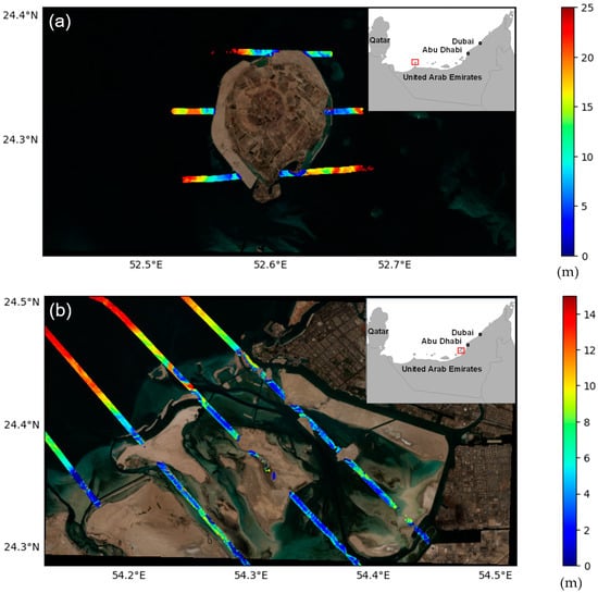
Figure 1.
Bathymetry field samples and the geo-boundaries investigated in this study around (a) Sir Bani Yas and (b) Abu Dhabi Islands. The red lines show the airborne echo-sounding path lines to measure bathymetry.
The second region was the Abu Dhabi Island and the waters surrounding it. The geographic location of this region has a range of latitude of 24.285°–24.506°N and longitude of 54.136°–54.511°E. This study area is also located in the southern region of the Arabian Gulf. While Abu Dhabi’s main district is situated on the island, there are many suburbs on the mainland. In addition, Abu Dhabi Island is surrounded by shallow water (i.e., within a depth of 25 m) and consists mainly of coral reefs, sands, sabkha, rocks, and coastal mangroves. Similar to the first study area, in situ bathymetric data are also available for this study area, which were used for the training and validation (Figure 1b).
3.2. Satellite Data Processing
In addition to the in situ bathymetry data, Copernicus Level-1C Sentinel-2A and Sentinel-2B images were used in this study. These images are freely available for download from the Sentinel Scientific Data Hub of the European Space Agency (ESA). Level-1C (L1C) products are top-of-atmosphere (TOA) products that have been corrected for radiometric and geometric errors. These corrections also include orthorectification and spatial registration using a global reference system (combined UTM projection and WGS84 ellipsoid), with a sub-pixel level of accuracy. Sentinel-2 has 12 bands ranging from the blue to the short-wave infrared (SWIR) at different spatial resolutions [20]. These images were obtained for both regions of the Abu Dhabi and Sir Bani Yas Islands, gathering different snapshots over 12 months, with no cloud conditions. These images were used to assess the temporal variability in bathymetry in both regions.
These Sentinel-2 images of all bands were processed using three different atmospheric correction methods, including Sen2Cor, ALOCITE, and the Case 2 Regional Coast Color process (C2RCC). These atmospheric correction methods removed the atmospheric effect from single-date Sentinel-2 Level-1C TOA products to produce Level-2A bottom-of-atmosphere (BOA) reflectance products. It was found that Sen2Cor (R2: 0.7, RMSE: 10.4) outperformed the other two methods, ALOCITE (R2: 0.6, RMSE: 13) and C2RCC (R2: −0.2, RMSE: 44) (results not shown), in the initial bathymetry comparisons. In addition to the atmospheric correction, the sunglint correction was performed using Hedley’s method. This method relies on the NIR (near-infrared region) to determine and correct the glint in visible wavelength bands [21]. As such, for each visible band, all the selected pixels were included in a linear regression of the NIR brightness (x-axis) against the visible band brightness (y-axis). According to Equation (1), all the pixels in a band can be deglinted if the slope of this line is bi:
where Ri is the pixel value in the band i, bi is the regression slope, RNIR is the pixel NIR value, and MinNIR is the ambient NIR level. Therefore, Sentienl-2 bands 2, 3, and 4 (used in this study) are corrected using band 8 of the same spatial resolution of 10 m. Figure 2 shows the RGB images of the Abu Dhabi region before and after deglinting.

Figure 2.
RGB images of Abu Dhabi regions (a) before sunglint correction and (b) after sunglint correction.
After considering the quality of the retrieved pixels, in order to ensure equal coverage across the two study areas, 600 points from the Sentinel-2 maps were randomly selected for match with the available in situ bathymetry data that would be used for the training of the models. In addition, 33% of the data (300 measurements) were taken in order to validate the SDB, following the common data splitting approach of around 70% for training and 30% for validation [22]. In order to examine the seasonal effect on the SDB performance, Sentinel-2 images from the 12 months of 2014 were considered for both study areas. Likewise, to further evaluate the effects of bio-productivity and sediments on the SDB performance, Sentinel-2-derived chlorophyll-a (Chl-a) and turbidity indicators and the depth attenuation coefficient Kd were retrieved for the same monthly scenes. These products were Sentinel-2 products that are derived based on the Chl-a OC3 algorithm [23] and Kd_480 [24,25].
3.3. Satellite-Derived Bathymetry Methods
In order to estimate the bathymetry, the linear and log-transformed ratio methods developed by Stumpf et al. (2003) [6] were used in addition to the new method proposed in this study, using the other Sentinel-2 bands trained through gradient boosting. Figure 3 shows the flow chart of the methodology implemented in this study, followed by detailed descriptions of each step involved.
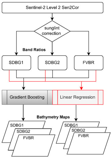
Figure 3.
Brief flowchart of the methodology implemented in this work. The linear regression method is presented in red color.
3.3.1. Linear and Log-Ratio Model
This model employs the ratios of linear and log-transformed water reflectance in bands with different water absorptions, so that the ratio varies with depth. Therefore, the atmospherically corrected remote sensing reflectance (Rrs) of Level-2 for the blue (443 nm and 490 nm) and green (560 nm) bands are used in this model. In addition, the log-transform is applied to account for the exponential decrease in light with depth. The SDB, hereinafter referred to as SDBgreen, is calculated using the ratio of green (λi) to blue (λj) bands:
where the satellite-derived pseudo-depth () is the dimensionless relative depth from satellite, while SDB is the satellite-derived bathymetry (meters). stands for the remote sensing reflectance, where is 560 nm and is 443 for SDBG1 or 490 nm for SDBG2, and are tunable constants used to transform the model results into actual depths, and n = 1000 is a fixed constant used to ensure that both logarithms are positive under any condition and that residual nonlinearity in the ratio is removed.
3.3.2. Four-Visible-Band Ratio (FVBR) Model
In this study, a new ratio was developed, called the four-visible-band ratio (FVBR), using the wavelengths B1-coastal aerosol (rescaled to 10 m), B2-blue, B3-green, and B4-red, which are less affected by light attenuation than longer wavelengths. The four ratios are a function of the Sentinel-2 bands B3/B1, B3/B2, B4/B1 and B4/B2. In order to model these ratios against the bathymetry, multi-linear regression and gradient boosting regression were employed. The coefficients of multi-linear regression were derived using the ordinary least squares method (OLS) [26]. On the other hand, gradient boosting is a machine learning technique used for classification and regression problems, which produces a prediction model by combining weak prediction models [27]. This technique entails the construction of a model in a stepwise fashion and enables the optimization of an arbitrary differentiable loss function. Gradient boosting was performed herein in Python using the XGBoost library (i.e., eXtreme Gradient Boosting). The XGBoost library is an optimized distributed gradient boosting library that is highly efficient, flexible, and portable. In addition, XGBoost is a parallel tree boosting algorithm that provides rapid and accurate solutions to many data science problems [28]. It includes the following steps:
Initialize the model with a constant value
Compute residuals
Train the regression tree with features x against r and create terminal node reasons
Compute
Update the model
4. Results
This section presents the analysis of the in situ bathymetry data collected by the multibeam echo sounder, followed by the estimation of the SDB using the methods discussed in Section 3.2. The maps of the estimated SDB were generated on a monthly basis, utilizing one bathymetry image per month. This enables the thorough examination of the temporal variation in the bathymetry estimates and the effects of water conditions, such as Chl-a and Kd, on the bathymetry estimations. These results are discussed in the following subsections.
4.1. In situ Bathymetry Analysis
Based on the in situ bathymetry data, the water around the Sir Bani Yas and Abu Dhabi Islands has depths of less than 25 m, with Abu Dhabi ranging between 0 and 14 m and Sir Bani Yas between 0 and 25 m, respectively. Accordingly, the average depth around Sir Bani Yas is approximately 12 m, whereas it is approximately 7 m around Abu Dhabi. However, more than 50% of Abu Dhabi’s water has depths greater than 6 m, whereas 25% of the water around Sir Bani Yas has depths ranging between 5 and 10 m, and 25% is greater than 15 m. Consequently, the depth around Sir Bani Yas has a higher standard deviation (std = 5.95 m) than that of Abu Dhabi Island (std: 3.91 m). Figure 4 shows the histograms of the field bathymetry data collected for the waters around the Sir Bani Yas and Abu Dhabi Islands.
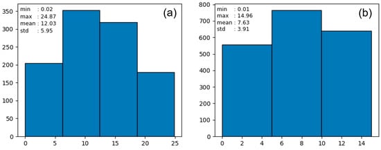
Figure 4.
Histograms of in situ bathymetry data collected by the multibeam echo-sounder around (a) the Sir Bani Yas and (b) Abu Dhabi Islands.
4.2. Comparison of Satellite-Derived and In Situ Bathymetries
The field echo-sounding bathymetry data were used to train and test the linear regression and gradient boosting methods. Both the linear regression and gradient boosting resulted in different levels of performances, meaning that an investigation of such variation in the estimations of the bathymetry was required. According to the R2 and RMSE values obtained through the linear and gradient boosting applied to SDBG1, SDBG2, and FVBR, the R2 generally ranged between 0.24 and 0.91, whereas the RMSE ranged between 2.98 and 24.55 (Figure 5). Specifically, the R2 obtained by the gradient boosting for the three ratios (R2: 0.24–0.91) outperformed the linear regression technique (R2: 0.3–0.84), as shown in Figure 5. This could be explained by the advantages of gradient boosting’s greater flexibility due to its hyper-parametrization and loss function, in addition to its capability to overcome the flaws in the data. However, the corresponding RMSE values for the gradient boosting were found to be somewhat higher (RMSE: 2.98–24.55 m) compared to that of the linear regression, with an RMSE of 5.14–22.45 m.
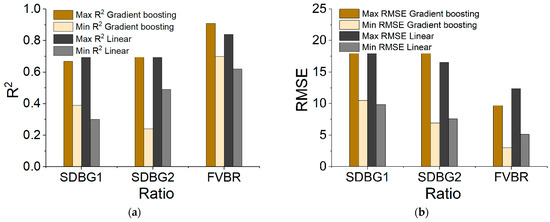
Figure 5.
Statistical values of (a) R2 and (b) RMSE for the three different ratios using both linear and gradient boosting.
The high RMSE value of 24.55 corresponds to the SDBG2 ratio for the month of January, when more than 50% of the values were overestimated. The SDBG2 model shows the worst performance compared to SDBG1 and FVBR. This could prove that the new ratios introduced in the FVBR approach represent the level of light penetration in the water by utilizing the four ratios instead of one ratio, whereby the aerosol band is used along with the three visible bands. Hence, the FVBR is found to be the best ratio for estimating the bathymetry, with an R2 greater than 0.7 and RMSE less than or equal to 12.36, especially when the gradient boosting method was applied. The SDBG1 is ranked as second-best to FVBR, and it could be applied in deep water where the sedimentation is not high. Figure 6 and Figure 7 show the matchup between the gradient boosting applied to the FVBR for different snapshots of the Sir Bani Yas and Abu Dhabi Islands over 12 months. Table 1 and Table 2 show the results of the R2 and RMSE after gradient boosting and linear regression were applied to the FVBR and SDBG2.
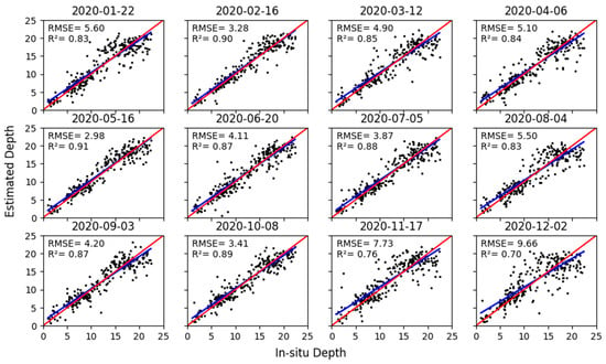
Figure 6.
Comparison between the in situ water depth (bathymetry) and estimated bathymetry values based on the gradient boosting applied using the FVBR approach for Sir Bani Yas Island. The red line is the 1:1 agreement line and the blue line is the model best fit.
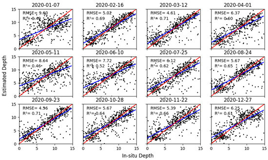
Figure 7.
Comparison between the in situ water depth (bathymetry) and estimated bathymetry values based on the gradient boosting applied using the FVBR approach for Abu Dhabi Island. The red line is the 1:1 agreement line and the blue line is the model best fit.

Table 1.
The results of the R2 and RMSE based on the gradient boosting and linear approach applied to FVBR.

Table 2.
The results of the R2 and RMSE based on the gradient boosting and linear approach applied to SDBG2.
5. Discussion
5.1. Temporal Variation in Bathymetry Estimates
The linear regression and gradient boosting techniques were used to estimate the bathymetry in the varying scenes over the 12-month period. This was performed in order to understand the temporal variation effect on the bathymetry estimates, including the effects of atmospheric factors, such as the dust level, in addition to the water conditions of bio-productivity, turbidity, and tidal patterns. Consequently, we retrieved Chl-a and Kd values, along with the bathymetry estimates. This can be explained by the high bio-productivity of the region (Chl-a exceeding 3 m mg−3) [29], as well as the high turbidity, particularly along the coasts [30]. Changes in the model’s performance over each month based on the linear regression and gradient boosting methods were analyzed in conjunction with the dust level, presented here according to the aerosol optical thickness (AOT), water turbidity, Chl-a content in the water, and tidal elevation.
As per the detailed comparison between the in situ and actual bathymetries for different snapshots taken over the 12-month period, upon assessing the accuracy of the retrieved bathymetry data obtained using both the linear regression and gradient boosting methods, it was found that R2 could drop below 0.6, especially for SDBG1 and SDBG2 during the winter months of November, December, and January, as shown in Figure 8. Interestingly, however, the FVBR model could overcome the temporal uncertainties found using these models, where R2 could drop during winter but still maintain values greater than 0.6. Both the linear regression and gradient boosting models resulted in the highest performances during the months of February, May, July, and September.
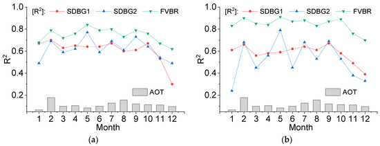
Figure 8.
Monthly time series of maximum R2 obtained for the three different ratios using (a) linear and (b) gradient boosting for estimating the bathymetry in both regions, Abu Dhabi and Sir Bani Yas Islands. The bar charts show the corresponding monthly AOT.
However, no clear correlation was found when comparing the R2 values of the retrieved bathymetry obtained by both linear regression and gradient boosting in conjunction with the aerosol levels measured as AOT. For example, when the AOT was high in February (e.g., around 0.2), the R2 values were found to be high, with an average of 0.7 for the three ratio models. However, when the AOT was low during March (e.g., less than 0.1), the R2 values were found to be low, especially for the SDBG1 and SDBG2 models, with an R2 of around 0.5. From this, we can interpret that increasing the AOT does not directly increase the bias in the bathymetry estimates for the three ratios. The explanation behind this interpretation is based on the systematic shift caused by the appearance of aerosols in the atmosphere. When using the ratio, this effect is canceled out and is not reflected in the modeled bathymetry. Therefore, using the band ratio is an advantage in overcoming the atmospheric intervention.
The accuracy of the bathymetry estimates was also cross-checked with the Chl-a and Kd to assess the sensitivity of the three ratios in regard to the sediments and biological productivity. In general, no significant correlations were observed between the estimated bathymetry and both Chl-a and Kd over the 12-month period for both regions. The Chl-a and Kd for Sir Bani Yas Island are shown in Figure 9 and Figure 10, respectively, along with the estimated bathymetry, shown in Figure 11. Likewise, the Chl-a and Kd values for Abu Dhabi Island are shown in Figure 12 and Figure 13, respectively, with the estimated bathymetry shown in Figure 14. This is considered a positive finding, since the bathymetry of the water is not affected significantly by changes in the surface turbidity and biological composition of the water, which were believed to contribute to a reduction in its precision. For instance, the Chl-a may reach up to 2 mg m−3 on the eastern side of the Sir Bani Yas Island compared to less than 1 mg m−3 on the western side, but this variation did not affect the bathymetry estimates, and no proportional tendency was observed. Similarly, in the region of Abu Dhabi Island, the Kd could exceed 1.4 in the inner channel water, but this did not increase the estimation of the bathymetry in these regions, where the bathymetry showed values ranging between 1 to 2 m.
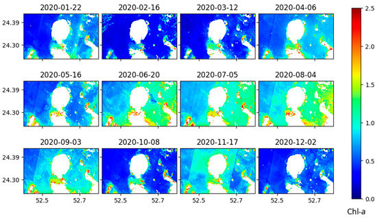
Figure 9.
Snapshots of the surface Chl-a over Sir Bani Yas Island, with a scale ranging from 0 to 2.5 mg m−3. The Chl-a is derived based on the OC3 algorithm using Sentinel-2 visible bands.
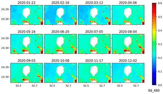
Figure 10.
Snapshots of the surface Kd_480 over Sir Bani Yas Island, with a scale ranging from 0 to 0.6 m−1. The Kd_480 is derived based on the algorithm of Lee et al., 2005 [25], using Sentinel-2 visible bands.
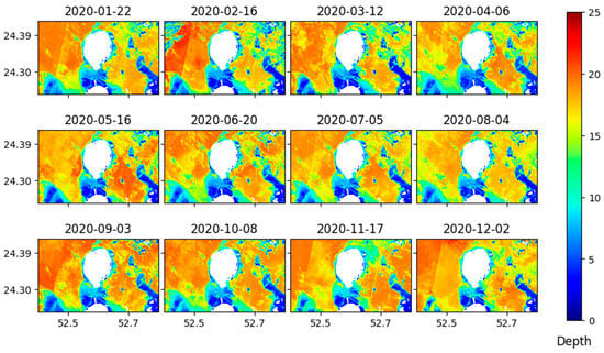
Figure 11.
Maps of satellite-derived bathymetry of the Sir Bani Yas Island based on the FVBR gradient boosting approach.
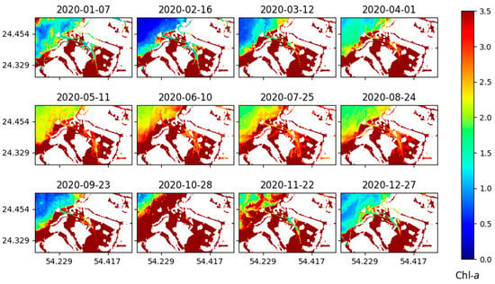
Figure 12.
Snapshots of the surface Chl-a over Abu Dhabi Island, with a scale ranging from 0 to 3.5 mg m−3. The Chl-a is derived based on the OC3 algorithm using Sentinel-2 visible bands.
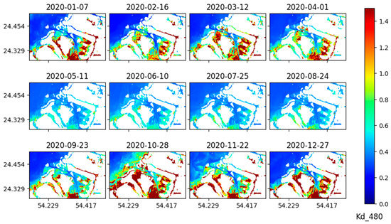
Figure 13.
Snapshots of the surface Kd_480 over Abu Dhabi Island, with a scale ranging from 0 to 1.4 m−1. The Kd_480 is derived based on the algorithm of Lee et al., 2005 [25], using Sentinel-2 visible bands.
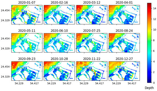
Figure 14.
Maps of satellite-derived bathymetry of Abu Dhabi Island based on the FVBR gradient boosting approach.
However, the reduction in R2 during the winter months, especially in the case of Sir Bani Yas Island, could be due to the surface currents or physical dynamics of the water, which significantly affect the surface sediments around the island. This is supported by the moderate wind density observed in the southern region of the Gulf during winter [31], when high sediments transport can occur [32]. These observations were found to be significant during December and January, when the lowest R2 values were found. In addition, the significant factors that can affect the estimation of the bathymetry were found to be the tidal elevation at the time of the collection of the in situ measurements and the overpass time of the satellite over the study areas. Based on the tidal elevation recorded during the sentinel image overpass [33], a high bias in the bathymetry results occurred when the tidal elevation was higher than 0.8 m, as shown in Figure 15. This was especially obvious for the month of January, when the tidal elevation reached 1.7 m during the satellite overpass. However, during May, July, and October, the R2 values were found to be high, and the corresponding tidal heights were at the lowest levels compared to the other months. The model was also found to perform better when the tidal pattern was semidiurnal, having two high tides and two low tides. However, when the tidal pattern was mixed, the modelled bathymetry was found to be less accurate. Oscillations of the tides can cause some surface changes in the bathymetry, especially in the coastal region, and should thus be taken into consideration when modeling the bathymetry.
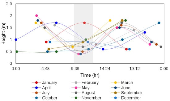
Figure 15.
Tidal elevation (height m) in Abu Dhabi for the twelve months. Some months shows two high and two low tides, whereas other months show either one high or low tide and two high/low tides. The gray shading indicates the overpass time window of Sentinel-2 over Abu Dhabi.
5.2. Satellite-Derived Bathymetry Maps
The final maps of the waters surrounding Sir Bani Yas Island and Abu Dhabi Island are shown in Figure 11 and Figure 14. The estimated bathymetry in Abu Dhabi shows ranges of less than 15 m, especially on the coastal side, where bathymetry does not exceed 5 m. This pattern was frequently observed over the entire 12-month period. When moving offshore, the bathymetry increased gradually, reaching up to 15 m. The offshore region was found to be dynamic in terms of the water depth, as the bathymetry fluctuated from time to time and was observed to be higher during specific months, such as February, March, June, July, and August. This high fluctuation in the bathymetry was caused by varying wave heights and surface water currents in the surface water. As for the Sir Bani Yas Island, the estimated bathymetry was higher than that of the Abu Dhabi region, which was expected. The range of the estimated bathymetry was below 25 m. The coastal side of Sir Bani Yas Island has a bathymetry ranging from around 2 to 6 m, whereas the offshore bathymetry ranged between 10 to 20 m depending on the month of retrieval. Similar to the Abu Dhabi region, it was found that the estimated bathymetry values can be affected by the water current and surface waves, thus causing fluctuations ranging from 1 to 2 m on a monthly basis.
5.3. Recommendations for Future Studies
As we found in this study, bathymetry varies and can be affected by temporal phenomena, such as sedimentation (to a certain extent), tidal elevation, water dynamics, and surface waves. Therefore, to accurately interpret the estimated bathymetry data, it is recommended to establish a system for keeping records of the aforementioned variables and to construct a robust dynamic model. In future studies, water currents could be obtained either from the current meters or from the ocean reanalysis data using the best spatial and temporal resolutions available. In addition, measurements of the Secchi disk depth would be useful for investigating the effect of water transparency on the estimated bathymetry data. It is also recommended that future researchers carry out a long-term sampling campaign to cover a full-year cycle, where most of the effects of seasonal changes on the collected data could be reflected, instead of limiting the study to a single season.
Moreover, since the surface water depth is significantly sensitive to the tidal height and oscillations, the scanning of the actual bathymetry should be performed at the overpass time of the satellite, when the tidal conditions are known. As for the scanning pattern, it is recommended to combine both the systematic sampling approach and randomly stratified sampling approach so that the developed model is influenced by the systemic patterns of the in situ measurements collected. Fortunately, in this work, the systematic pattern of the in situ bathymetry data was not affected the predicted snapshots of the bathymetry in both regions, given the homogeneous distribution of the bathymetry in the regions. However, stratified random sampling is strongly recommended for other regions where the bathymetry varies significantly.
6. Conclusions
The bathymetry in coastal regions with water depths not exceeding 25 m was estimated in this work. Sentinel-2 visible bands were used to obtain the conventional SDB (green to blue) ratio in addition to the newly proposed four-band ratio (FVBR). Three atmospheric correction methods were applied, and Sen2Cor outperformed the other two methods, ALOCITE and C2RCC, in estimating the bathymetry. Two data model approaches were used, including linear regression and gradient boosting for both the blue/green ratio and the FVBR. The results show that the proposed ratio can better predict and estimate the bathymetry compared to the conventional blue to green ratio. This can be explained by the additional features of the water transparency extracted from the additional aerosol and red bands, which are considered in the new proposed ratio.
As for the data model approach, gradient boosting was found to produce better outcomes compared to linear regression, with improvements in the bathymetry estimation exceeding 30%. The sensitivity analysis of the bathymetry errors and the other parameters suggests that Chl-a, Kd, and the atmospheric dust level do not significantly affect the bathymetry estimation. This happens only during specific events, where sediments may be driven by the strong seasonal water currents, thereby affecting the accuracy of the bathymetry estimation. Additionally, the estimation of the bathymetry was found to be significantly affected by the tidal oscillations, especially in the shallow coastal regions. Therefore, it is recommended to record the tidal conditions at the echo-sounding scanning locations so as to accurately assess the effect of tides and to plan the echo-sounding study so that it coincides with the satellite overpass time.
Author Contributions
Conceptualization, F.A.G., M.R.A.-S., C.-S.C. and H.G.; Formal analysis, F.A.G. and M.R.A.-S.; Investigation, F.A.G. and M.R.A.-S.; Methodology, F.A.G., M.R.A.-S. and C.-S.C.; Resources, M.R.A.-S. and H.G.; Validation, F.A.G.; Writing—original draft, M.R.A.-S.; Writing—& editing, M.R.A.-S. and C.-S.C. All authors have read and agreed to the published version of the manuscript.
Funding
This research was funded by Khalifa University, grant number FSU-2020-017.
Data Availability Statement
The Chl-a data are available at https://oceancolor.gsfc.nasa.gov/atbd/chlor_a/ (accessed on 20 August 2022) and the Kd data are available at https://oceancolor.gsfc.nasa.gov/atbd/kd_490/ (accessed on 20 August 2022).
Acknowledgments
The authors would like to thank Khalifa University for the financial support of this project. The authors would like to thank Mubadala (BAYANAT) for providing the bathymetry data.
Conflicts of Interest
The authors declare no conflict of interest.
References
- Dissanayake, P.; Yates, M.L.; Suanez, S.; Floc’h, F.; Krämer, K. Climate Change Impacts on Coastal Wave Dynamics at Vougot Beach, France. J. Mar. Sci. Eng. 2021, 9, 1009. [Google Scholar] [CrossRef]
- Kirezci, E.; Young, I.R.; Ranasinghe, R.; Muis, S.; Nicholls, R.J.; Lincke, D.; Hinkel, J. Projections of Global-Scale Extreme Sea Levels and Resulting Episodic Coastal Flooding over the 21st Century. Sci. Rep. 2020, 10, 1–12. [Google Scholar] [CrossRef] [PubMed]
- Xu, L.; Ding, S.; Nitivattananon, V.; Tang, J. Long-Term Dynamic of Land Reclamation and Its Impact on Coastal Flooding: A Case Study in Xiamen, China. Land 2021, 10, 866. [Google Scholar] [CrossRef]
- Ibrahim, H.D.; Xue, P.; Eltahir, E.A.B. Multiple Salinity Equilibria and Resilience of Persian/Arabian Gulf Basin Salinity to Brine Discharge. Front. Mar. Sci. 2020, 7, 573. [Google Scholar] [CrossRef]
- Yagoub, M.M.; Kolan, G.R. Monitoring Coastal Zone Land Use and Land Cover Changes of Abu Dhabi Using Remote Sensing. J. Indian Soc. Remote Sens. 2006, 34, 57–68. [Google Scholar] [CrossRef]
- Stumpf, R.P.; Holderied, K.; Sinclair, M. Determination of Water Depth with High-resolution Satellite Imagery over Variable Bottom Types. Limnol. Oceanogr. 2003, 48, 547–556. [Google Scholar] [CrossRef]
- Casal, G.; Monteys, X.; Hedley, J.; Harris, P.; Cahalane, C.; McCarthy, T. Assessment of Empirical Algorithms for Bathymetry Extraction Using Sentinel-2 Data. Int. J. Remote Sens. 2019, 40, 2855–2879. [Google Scholar] [CrossRef]
- Poursanidis, D.; Traganos, D.; Reinartz, P.; Chrysoulakis, N. On the Use of Sentinel-2 for Coastal Habitat Mapping and Satellite-Derived Bathymetry Estimation Using Downscaled Coastal Aerosol Band. Int. J. Appl. Earth Obs. Geoinf. 2019, 80, 58–70. [Google Scholar] [CrossRef]
- Hamylton, S.M.; Hedley, J.D.; Beaman, R.J. Derivation of High-Resolution Bathymetry from Multispectral Satellite Imagery: A Comparison of Empirical and Optimisation Methods through Geographical Error Analysis. Remote Sens. 2015, 7, 16257–16273. [Google Scholar] [CrossRef]
- Wang, C.-K.; Philpot, W.D. Using Airborne Bathymetric Lidar to Detect Bottom Type Variation in Shallow Waters. Remote Sens. Environ. 2007, 106, 123–135. [Google Scholar] [CrossRef]
- Sagawa, T.; Yamashita, Y.; Okumura, T.; Yamanokuchi, T. Satellite Derived Bathymetry Using Machine Learning and Multi-Temporal Satellite Images. Remote Sens. 2019, 11, 1155. [Google Scholar] [CrossRef]
- Najar, M.A.; Benshila, R.; Bennioui, Y.E.; Thoumyre, G.; Almar, R.; Bergsma, E.W.J.; Delvit, J.-M.; Wilson, D.G. Coastal Bathymetry Estimation from Sentinel-2 Satellite Imagery: Comparing Deep Learning and Physics-Based Approaches. Remote Sens. 2022, 14, 1196. [Google Scholar] [CrossRef]
- Niroumand-Jadidi, M.; Bovolo, F.; Bruzzone, L. SMART-SDB: Sample-Specific Multiple Band Ratio Technique for Satellite-Derived Bathymetry. Remote Sens. Environ. 2020, 251, 112091. [Google Scholar] [CrossRef]
- Pereira, P.; Baptista, P.; Cunha, T.; Silva, P.A.; Romão, S.; Lafon, V. Estimation of the Nearshore Bathymetry from High Temporal Resolution Sentinel-1A C-Band SAR Data—A Case Study. Remote Sens. Environ. 2019, 223, 166–178. [Google Scholar] [CrossRef]
- Bergsma, E.W.J.; Almar, R.; Rolland, A.; Binet, R.; Brodie, K.L.; Bak, A.S. Coastal Morphology from Space: A Showcase of Monitoring the Topography-Bathymetry Continuum. Remote Sens. Environ. 2021, 261, 112469. [Google Scholar] [CrossRef]
- Wang, L.; Liu, H.; Su, H.; Wang, J. Bathymetry Retrieval from Optical Images with Spatially Distributed Support Vector Machines. GIScience Remote Sens. 2019, 56, 323–337. [Google Scholar] [CrossRef]
- Misra, A.; Vojinovic, Z.; Ramakrishnan, B.; Luijendijk, A.; Ranasinghe, R. Shallow Water Bathymetry Mapping Using Support Vector Machine (SVM) Technique and Multispectral Imagery. Int. J. Remote Sens. 2018, 39, 4431–4450. [Google Scholar] [CrossRef]
- Mateo-Pérez, V.; Corral-Bobadilla, M.; Ortega-Fernández, F.; Vergara-González, E.P. Port Bathymetry Mapping Using Support Vector Machine Technique and Sentinel-2 Satellite Imagery. Remote Sens. 2020, 12, 2069. [Google Scholar] [CrossRef]
- Dredging Today Unique System Installs Kongsberg EM 2040 Multibeam Echo Sounder on Bayanat Vessels. Available online: https://www.dredgingtoday.com/2014/07/02/unique-system-installs-kongsberg-em-2040-multibeam-echo-sounder-on-bayanat-vessels/ (accessed on 20 August 2022).
- Ody, A.; Doxaran, D.; Vanhellemont, Q.; Nechad, B.; Novoa, S.; Many, G.; Bourrin, F.; Verney, R.; Pairaud, I.; Gentili, B. Potential of High Spatial and Temporal Ocean Color Satellite Data to Study the Dynamics of Suspended Particles in a Micro-Tidal River Plume. Remote Sens. 2016, 8, 245. [Google Scholar] [CrossRef]
- Hedley, J.D.; Harborne, A.R.; Mumby, P.J. Simple and Robust Removal of Sun Glint for Mapping Shallow-Water Benthos. Int. J. Remote Sens. 2005, 26, 2107–2112. [Google Scholar] [CrossRef]
- Gholamy, A.; Kreinovich, V.; Kosheleva, O. Why 70/30 or 80/20 Relation between Training and Testing Sets: A Pedagogical Explanation. In Departmental Technical Reports (CS); University of Texas at El Paso: El Paso, TX, USA, 2018. [Google Scholar]
- NASA Chlorophyll a (Chlor_a). Available online: https://oceancolor.gsfc.nasa.gov/atbd/chlor_a/ (accessed on 20 August 2022).
- NASA Diffuse Attenuation Coefficient for Downwelling Irradiance at 490 Nm (Kd_490). Available online: https://oceancolor.gsfc.nasa.gov/atbd/kd_490/ (accessed on 20 August 2022).
- Lee, Z.; Du, K.; Arnone, R. A Model for the Diffuse Attenuation Coefficient of Downwelling Irradiance. J. Geophys. Res. Ocean. 2005, 110. [Google Scholar] [CrossRef]
- Escoto, J.E.; Blanco, A.C.; Argamosa, R.J.; Medina, J.M. Pasig River Water Quality Estimation Using an Empirical Ordinary Least Squares Regression Model of Sentinel-2 Satellite Images. Int. Arch. Photogramm. Remote Sens. Spat. Inf. Sci. 2021, 46, 161–168. [Google Scholar] [CrossRef]
- Natekin, A.; Knoll, A. Gradient Boosting Machines, a Tutorial. Front. Neurorobot. 2013, 7, 21. [Google Scholar] [CrossRef]
- XGBoost XGBoost Documentation. Available online: https://xgboost.readthedocs.io/en/latest/index.html%0Ahttps://xgboost.readthedocs.io/en/latest/#%0Ahttps://xgboost.readthedocs.io/en/latest/ (accessed on 20 August 2022).
- Al-Shehhi, M.R.; Nelson, D.; Farzanah, R.; Alshihi, R.; Salehi-Ashtiani, K. Characterizing Algal Blooms in a Shallow & a Deep Channel. Ocean Coast. Manag. 2021, 213, 105840. [Google Scholar]
- Al Kaabi, M.R.; Zhao, J.; Ghedira, H. MODIS-Based Mapping of Secchi Disk Depth Using a Qualitative Algorithm in the Shallow Arabian Gulf. Remote Sens. 2016, 8, 423. [Google Scholar] [CrossRef]
- Al-Salem, K.; Neelamani, S.; Al-Nassar, W. Wind Energy Map of Arabian Gulf. Nat. Resour. 2018, 9, 212–228. [Google Scholar] [CrossRef]
- Al-Ghadban, A.N.; Massoud, M.S.; Abdali, F. Bottom Sediments of the Arabian Gulf: I. Sedimentological Characteristics. Kuwait J. Sci. Eng. 1996, 23, 71–88. [Google Scholar]
- Tides4fishing. Available online: https://tides4fishing.com/ae/united-arab-emirates/abu-dhabi (accessed on 10 August 2022).
Publisher’s Note: MDPI stays neutral with regard to jurisdictional claims in published maps and institutional affiliations. |
© 2022 by the authors. Licensee MDPI, Basel, Switzerland. This article is an open access article distributed under the terms and conditions of the Creative Commons Attribution (CC BY) license (https://creativecommons.org/licenses/by/4.0/).