A New Approach to Satellite-Derived Bathymetry: An Exercise in Seabed 2030 Coastal Surveys

Abstract

ARGANS has years of experience in analysing the factors limiting light transmission in coastal environments around the world. This has led its Satellite-Derived Bathymetry (SDB) team to the conclusion that current satellite instruments and their resolution are unable to provide the absolute precision required for safe navigation according to International Hydrographic Bureau (IHO) standards, except in the clearest of waters characterised by sufficiently well-defined environmental parameters. This limitation is caused by the variability itself of the parameters in the radiative transfer equation (RTE), which is too high to provide results within the strict accuracy ranges of IHO S.44, as shown by scatter plots characterised time and again by large biases and standard deviations of several metres. The radiative transfer equation and Hydrolight simulations are not at fault, but their results must be interpreted with extreme caution if the level of accuracy required for safe navigation over large areas is to be guaranteed. Therefore, ARGANS has developed an innovative, alternative method. This is based on the classification of the full range of images pixels allowing for homogeneous sub-areas to be determined and linked together by artificial intelligence and statistical clustering of similar parameters. Thanks to the sponsorship of the European Space Agency and Seabed 2030, ARGANS has been able to test its Water Column Parameter Estimator (WCPE), first in the challenging waters of Madagascar updating over 1000 km of lead line exploratory surveys, then in the South Pacific coral environment and then in the turbid coastal water of Qatar. The parameters determined by WCPE can be extrapolated to unknown regions of similar environment and propagated from one place to the next, using a chain method somewhat inspired by photogrammetric techniques of old. Further progress and automation can be expected from an improved control of sediment plumes that can obscure or distort all optical methods, whether satellite or LIDAR.

1. Introduction

Fifty Years of SDB Theory, Trials, and Developments

Preceded by 20 years of theoretical studies and field simulations, SDB is a story of persistence interspersed with phases of hope and delusion that took shape officially in 1990 with the introduction of the first space chart (Figure 1) into a national catalogue.

Today, the tone amongst SDB users and service providers is optimistic, and very much in line with our 2015 former projection (Figure 2), unfortunately no longer applicable.

In short, SDB products are expected to meet someday the IHO/S-44 accuracy standards. With this projection taken for granted, the best-intentioned, but not necessarily the best-informed, Hydrographic Offices are now demanding 2-m resolution grid data, as if satellite imagery could provide the same kind of accuracy as the multibeam echo sounders that took 20 years to certify, and in doing so, end up possibly spending half the cost of optical surveys to acquire high-resolution imagery from satellite constellations that were originally designed to provide accurate information of land features, not of low-reflectance coastal waters.

Encouraged by the traditional scepticism of their fellow hydrographers, ARGANS scientists are once again challenging this optimistic trend and, after years of failing to force SDB to produce consistently S-44 compliant results (Figure 3), except in very small areas supported by accurate ground truth, and further attempts to complete the current theories and operate the best satellite constellations, they have concluded that SDB current practices are unlikely to meet this wishful thinking and must be redesigned almost from scratch.

The Radiative Transfer Equation of Lee et al. is not at fault, nor are the ever-improving satellite constellations and sensors, but analysts keep coming back to the intrinsic weakness of the SDB which has never been fully addressed, namely its inability to differentiate between deep-water reflectance on a light background and shallow-water reflectance on a dark seafloor, expressed decades ago by Dr. Hedley’s popular image depicted at Figure 4. Still active in SDB, Dr Hedley, a former ARGANS Developer, has founded his own company, Numerical Optics Ltd., who owns Hydrolight, a model used by all SDB specialists.

One may observe that the classical laws of physics being essentially mathematical in formulation cannot reflect the complexity of nature’s phenomena which, although being extremely diverse, are neither chaotic nor random. From this diversity structures and patterns can emerge, statistical in nature, that can be incorporated into models that scientists, helped by the advent of Big Data gathering systems, can now develop.

The need to introduce intelligent interpretations of coherent clusters to eliminate uncharacteristic depths from their Terrain Models led our developers to focus on correlations and statistical analysis rather than repeating at nauseam the Lee et al. inversion mechanism. Statistics is seen as a bridge between the apparent diversity of nature and the underlying physical laws.

Not only does SDB have the potential to yield depths, but these depths should be associated with better probabilities of occurrence so that, for instance, a 15 m deep pixel should be semi-automatically eliminated from a 5-m-deep rocky plateau, or worse, a 10 m potentially dangerous outcrop should not be ignored in an apparently safe 15 m environment.

Rather than forcing the limited Lee et al. equations to provide an unattainable absolute accuracy to ensure safe navigation in the then West Indies project, ARGANS Developers decided three years ago to return to their drawing board and elaborate an alternative method based on statistical analysis of the full range of image pixels propped up by artificial intelligence, while retaining the light attenuation principles of RTE-based traditional models.

The point of this paper is to show that, whilst S-44 orders of precision are still out of reach in large areas, no matter the amount of public money spent, SDB properly revisited can yield reliable depths at affordable cost and can fill the coastal gaps that GEBCO/Seabed 2030 is looking for with a near-metric precision never attained before.

The tool designed to attain the Seabed 2030 almost altruistic goal of 100% seafloor coverage is called the Water Column Parameter Estimator, further theorised in Chapter IV under its acronym: WCPE.

2. State-of-the-Art

A full presentation on the SDB State-of-the-Art has been made in an article [1] published in 2020 by the International Hydrographic Review.

The present Remote Sensing article has been conceived originally as a complement to this earlier peer-reviewed publication, providing visibility and continuity on the development of SDB from the origin in the late 1970s by some of the hydrographers who pioneered the methodology and introduced it to the hydrographic world.

In a nutshell, SDB progressed along the following phases, involving a growing number of international players:

• Before 1983: SDB early trials and field simulations by the French Hydrographic Office. Funded by the Ministry of Defence, these trials were validated by a number of internal reports such as [2] “Study of the bathymetric applications of a blue channel radiometer on board a satellite, using data from an airborne simulation” (1983).
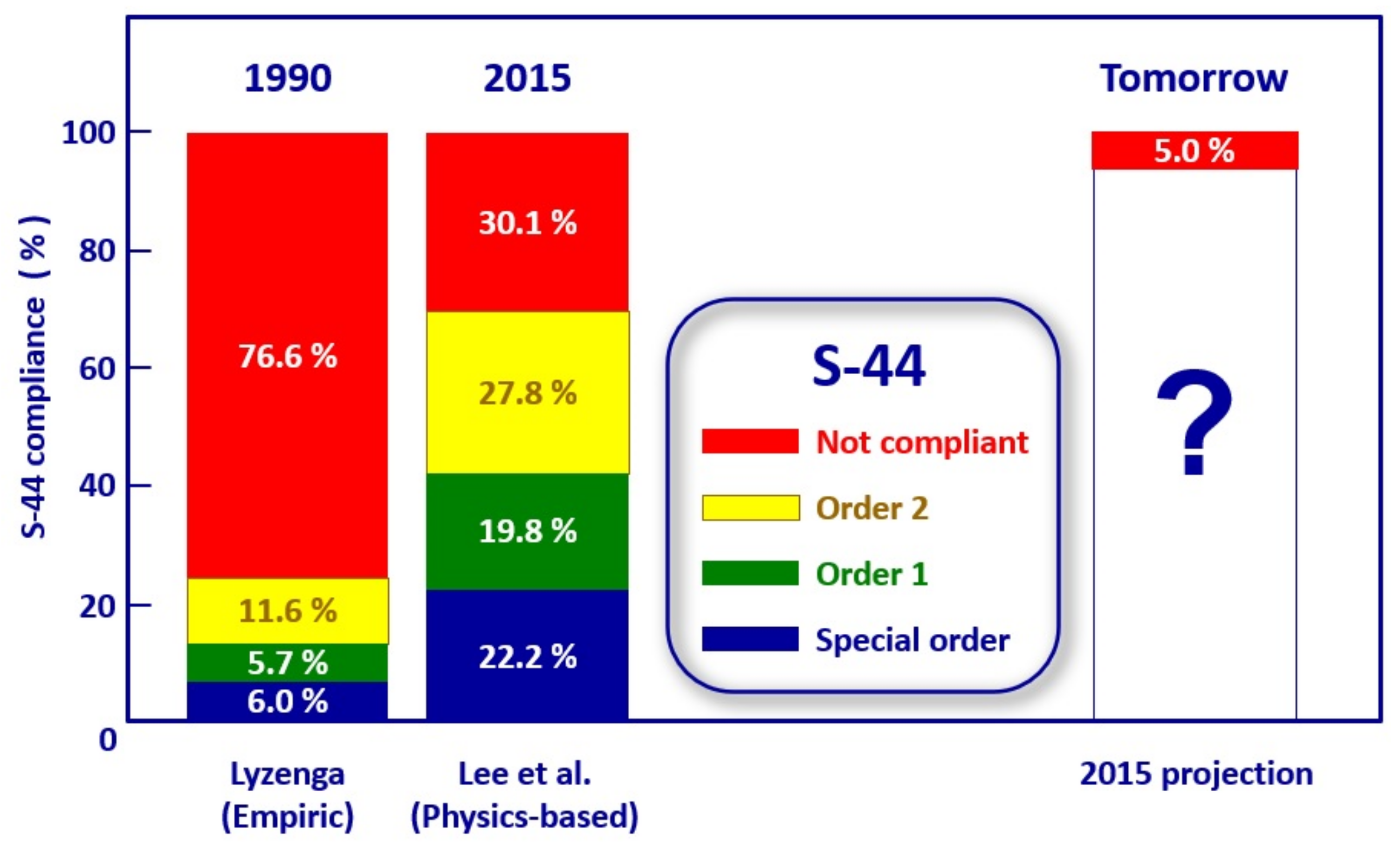
• 1980–1990: Development and implementation of the Lyzenga empiric method in the coral waters of New Caledonia and French Polynesia.
• 1990: First publication of the SDB chart of Ouvea in a national chart series.
• 1990–2019: Dissemination of SDB worldwide and subsequent implementation of the Lee et al. physics-based method. SDB methodology spreads amongst HOs and commercial service providers.
• 2019–2022: Introduction in the UK of a statistical method backed by machine learning to complement the traditional SDB methodologies.

3. Objectives

A Novel SDB Approach Based on the Exploitation of Statistics

Following the lessons learnt from a 2018 ESA-sponsored survey which had established once more that the traditional SDB software derived from the Lee et al. formula was too limited to describe the seafloor bathymetry properly and abide by the IHO S-44 standards of precision, it was attempted to develop an entirely new approach, based on statistics, to analyse and reduce the biases and discrepancies revealed by spread out cross sections and scatterplots of satellite images, as exemplified in Figure 5 below.

The new method, dubbed WCPE for Water Column Parameters Estimator, is a statistical tool based on successive approximations that allow the ROI’s sub-areas to be linked together by statistical clustering of similar parameters, leading to the most probable selection of depths amongst SDB’s vast number of solutions. Artificial intelligence is widely used to train the model by determining the multiple classes highlighted in the ROI’s density profiles (Figure 6), and not only to optimise empirical matching between model and ground truths. In short, SDB has moved from trying to determine a unique, but noisy and imprecise, solution to an analysis of clusters, each associated with a probability.

WCPE relies on the same Radiative Transfer Equation as all previous empiric and physics-based methods (Figure 7) but adds to them a statistical clustering tool that allows for automatic determination of the types of coastal waters characterised by their set of associated parameters such as seafloor reflectance, water IOPs, DOP, etc., all backed by error figures, crucial for analysis and exploitation.

Once the AOI distribution has been analysed and the characteristic parameters sorted out, the parameters in question can be extracted with their probability of occurrence (see Figure 8).

Thanks to an initial sponsorship by Seabed 2030, followed by a further R&D contract provided by an Oil Supermajor, ARGANS was able to explore WCPE in West Indies then test it in Madagascar’s challenging waters and partially complete 1300 km of lead line and exploratory surveys carried out a century ago (Figure 9). This first experience was extended to the textbook case of a South Pacific atoll, then further applied to the tricky Qatar waters to validate a DTM developed specially to provide safety of navigation to the deployment of towed arrays.

These extensive tests not only proved that the statistic approach delivers results better or at least comparable with those of traditional RTE methods but further provided a wealth of information that is normally out of reach of more restricted traditional procedures. Thanks to statistics and comparisons, for instance, a better qualified opinion on the selection of images could be made that should be of great consequence when one must select the best satellite images to produce nautical charts at an optimised cost.

The first beneficiary should be the GEBCO and those users who cannot afford to purchase commercial images, especially when proved ill-suited to maritime applications.

4. WCPE Method

Note: due to the complexity of this section, standard paragraph numbering has been introduced.

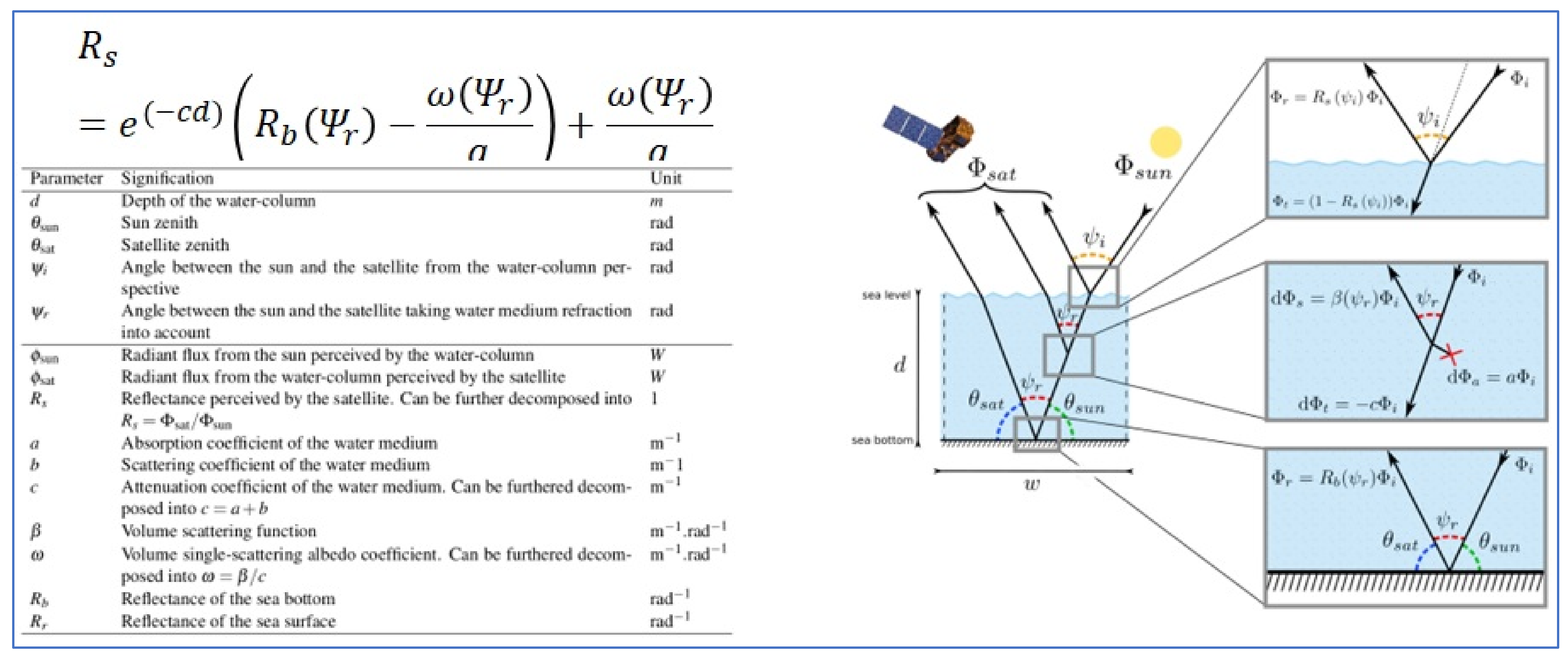
4.1. Starting Point and Scope

For the world brigade of SDB Specialists, the main postulate upon which the WCPE method was built is that the base equations derived in 1970 [3] by Polcyn then in 1975 by Lyzenga [4] constitute the undisputed foundation. Case in point: those equations are still relevant nowadays and appears one way or another at the core of every SDB method used ever since. Save for pure machine learning methods, but it can be construed that their internal model tries to approximate a solution to those equations.

$$L\left(h\right)=L_s+L_b{e}^{\alpha h}$$

(1)

WCPE uses this formula as its basis not because it is popular, but because it exhibits many interesting properties:

• It bundles up all the main meaningful physical parameters scientists are interested in.
• It is easy to invert to estimate the depth.
• It is valid for every spectral band (although some are marginally better to use than others).
• It is free of arbitrary empirical coefficients.

Over the course of 50 years, the whole field of SDB spent considerable effort trying to palliate some of the problems inherent to that formula. The main ones being:

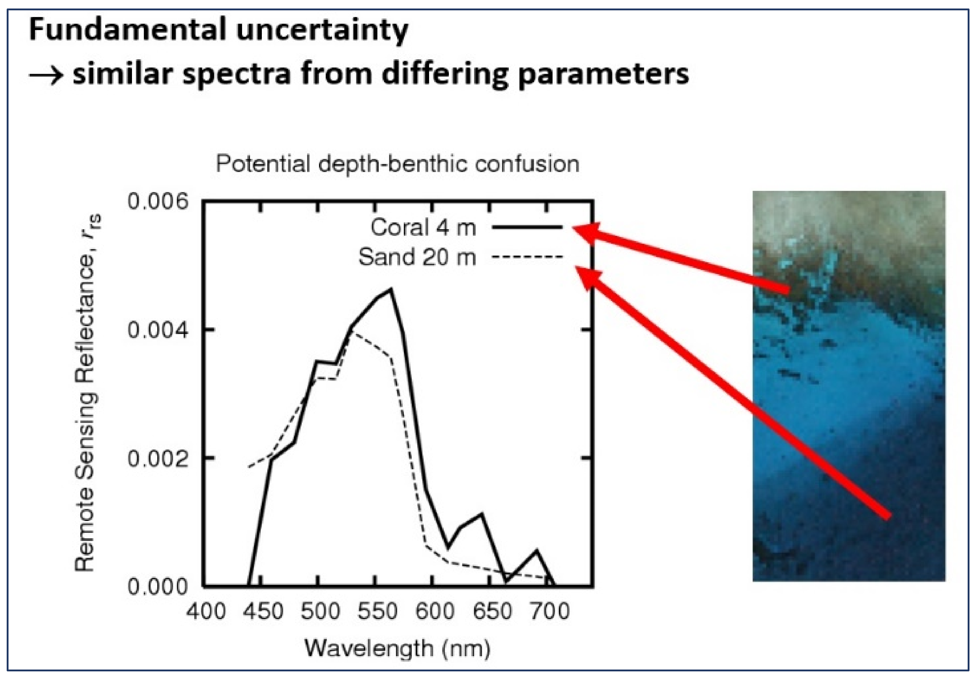
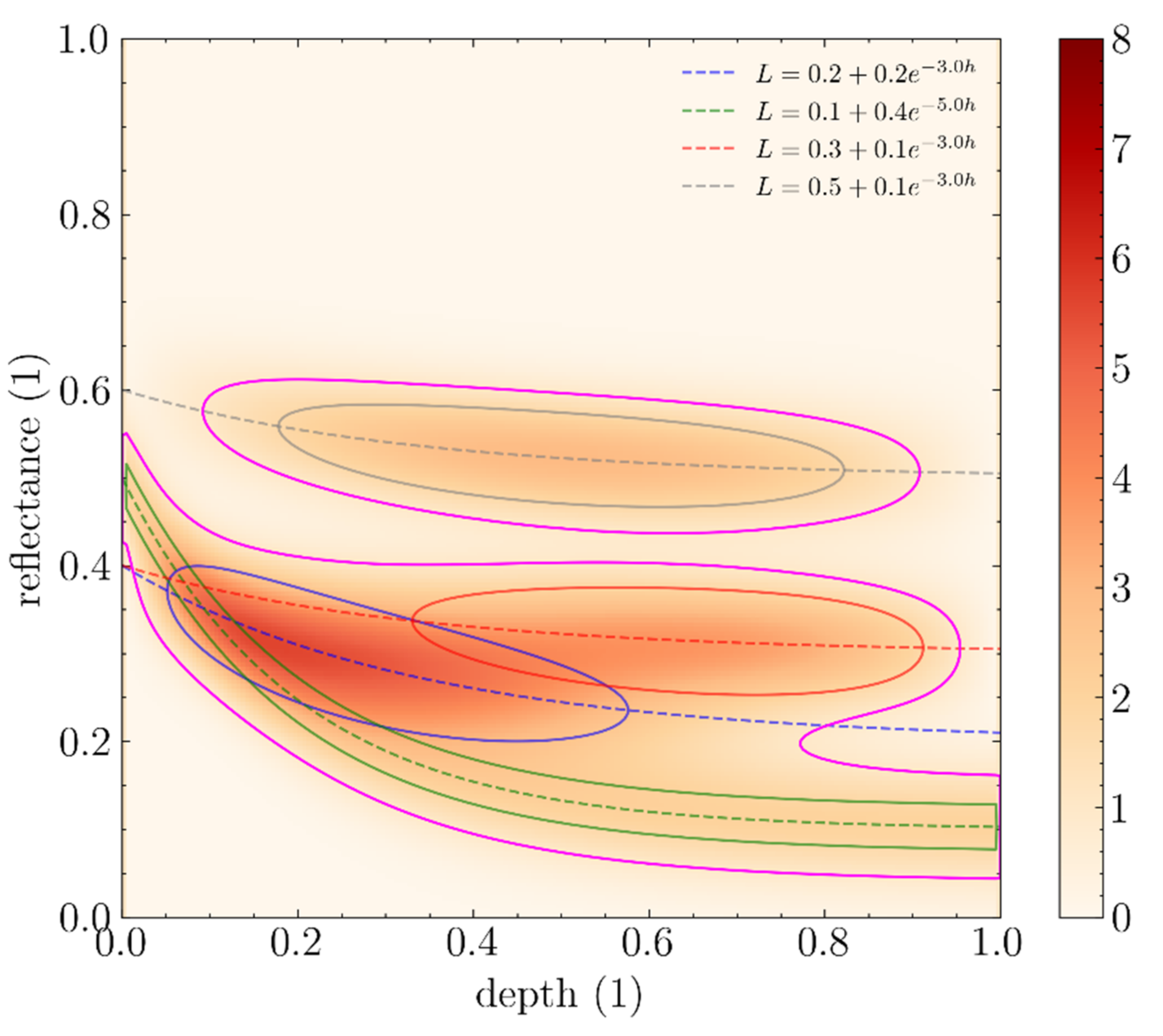
• The first problem: as seen earlier, certain water-column profiles may exhibit the same radiance but have incompatible depths, thus leading to ambiguities about the resulting bathymetry.
• The second problem: when trying to retrieve depths, several a priori are required because the equation is severely underdetermined and unresolved members must be parameterised. Some of those parameters are very difficult to obtain, e.g., attenuation coefficients, seafloor reflectances).
• Other difficulties that add to the challenge of deriving bathymetry include:
• Proper calibration of satellite images.
• Proper removal of atmospheric effects in coastal environments.

However, those are independent of the model used so they will not be considered in this paper.

The main way to solve the first problem is to consider several spectral bands instead of just one (David R. Lyzenga and Tanis, n.d.), and use the increase in dimensionality to help distinguish between ambiguous profiles. The bands effectively used are the red, green, and blue bands, available on all satellites providing true colour imagery. Although this method allows to separate many ambiguous cases, the main limitation has now shifted to the number of bands used and the fact that some profiles cannot be distinguished by the spectral signature alone, however many bands you have. The framework for a potential solution to problem 1 will be briefly laid out at the end of this section, but it will not be the focus of this article.

Problem 2 is another very challenging issue. In situ data is very costly to collect and usually require field interventions. Extremely specific physical parameters such as attenuation coefficients and seafloor reflectances are even more difficult to collect than actual depths. Attempts include leveraging scientific tools and databases such as Hydrolight [5] developed in accordance with. Zhongping Lee, Curtis Mobley, and [6] John Hedley, to find values to assign to missing parameters in the model. One can also try to reduce the number of in situ data needed to build an inversion model by finding judicious approximations to weaken the set of equations in a way that allows its parameters to be regressed using only a few parameters, such as depths and radiance only [7] re. David R. Lyzenga and Tanis. The first attempt is limited by the number of water-column and seafloor profiles studied and catalogued. It also still requires a human operator to decide which material samples correspond best to the ones found in the area studied. The second attempt is limited by the fact that the formula now transformed into a weakened form reduces the relevance and accuracy of the resulting bathymetry.

The WCPE method and software have been designed and implemented to provide a solution to the 2nd problem that does not rely on using parameters from external material databases and does not require to weaken the main formula. To do that, statistical tools were employed to bridge between the idealised and rigid nature of the base equations and the great diversity of spectral profiles commonly found in satellite images. It will be shown that despite cutting some slack in the selection of the parameters to be included in the model and the number of approximations to make them workable, the problem of requiring a lot of in situ data to build up models is still present in WCPE. The methods used to mitigate this costly requirement will be discussed below. A very important assumption that will be used throughout this section is that we dispose of some in situ depths and reflectances to use to create bathymetry models.

Before detailing the mathematical framework behind the WCPE method, the following simplification and change in notation is used to keep things simple: the range of depth considered will be supposed finite and capped by a higher bound $h_{max}\in ℝ+$. An arbitrary depth within this range can then be normalised within [0, 1] by dividing by $h_{max}$. The Lyzenga equation in the rest of this section will be used with the following form:

$$L\left(h\right)=a+b{e}^{-ch},h\in {ℝ}_{+}$$

(2)

where $h$ is the normalised depth value mentioned above and $a$, $b$, $c$ are derived from the parameters in the original Lyzenga’s equation, accounting for the fact that $h$ has been normalised.

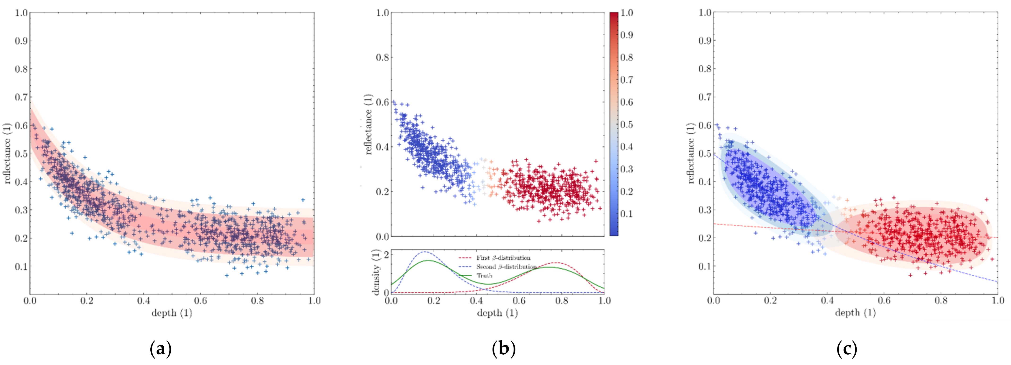
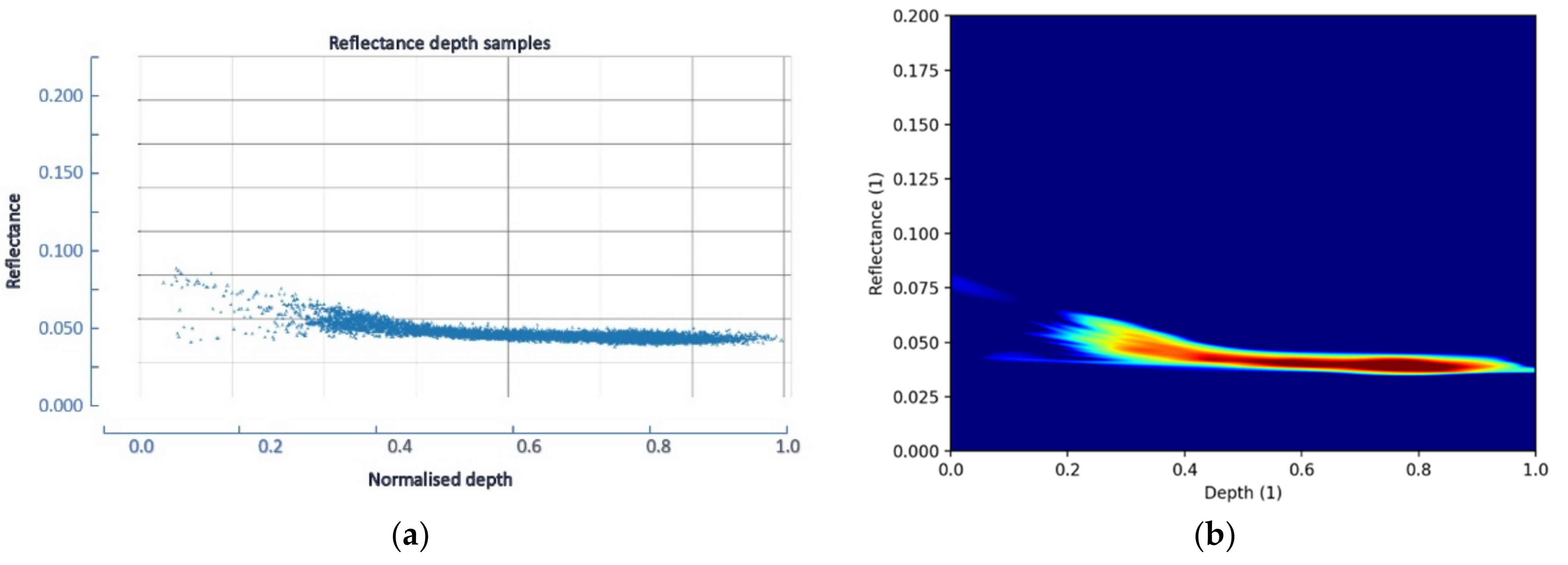
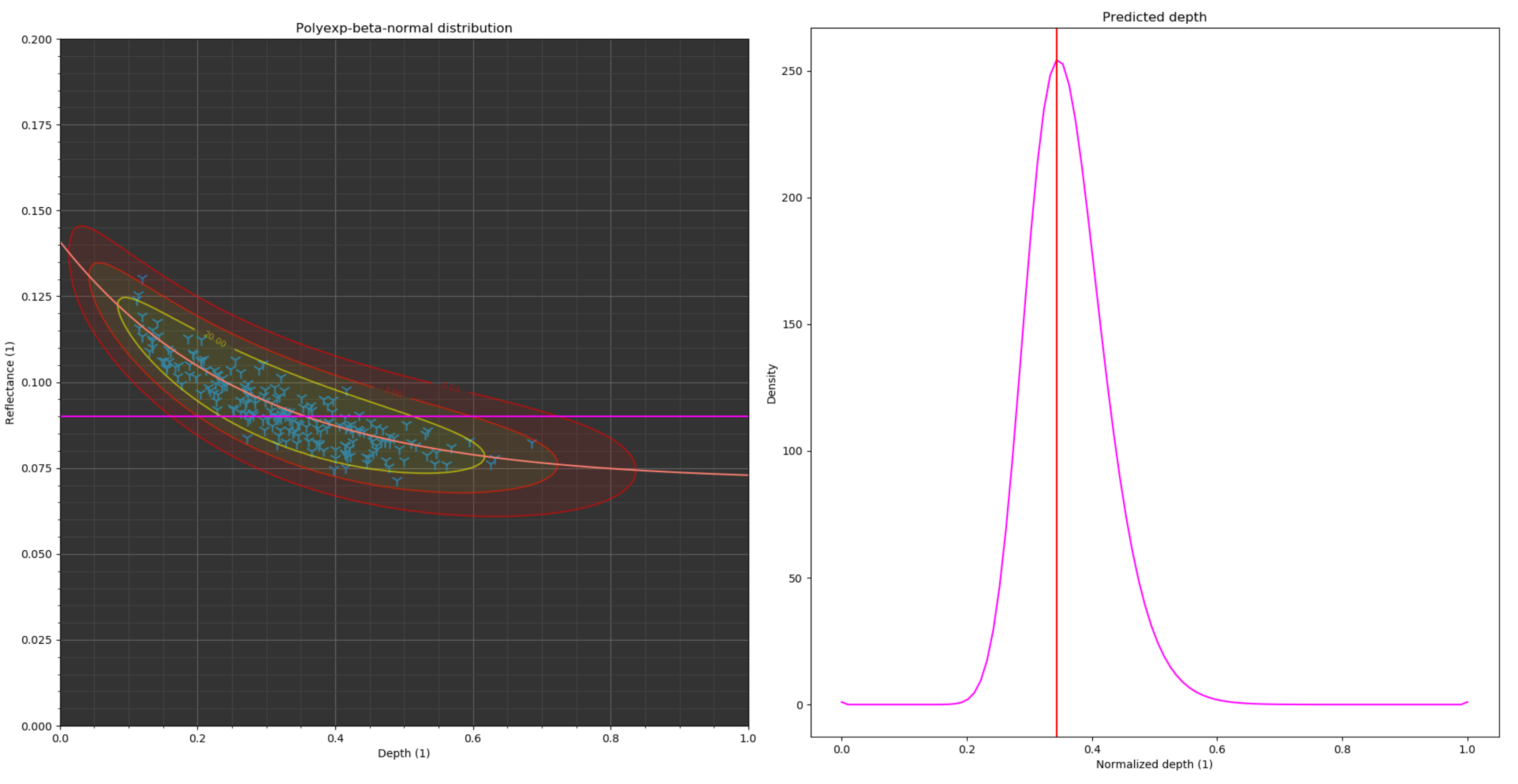
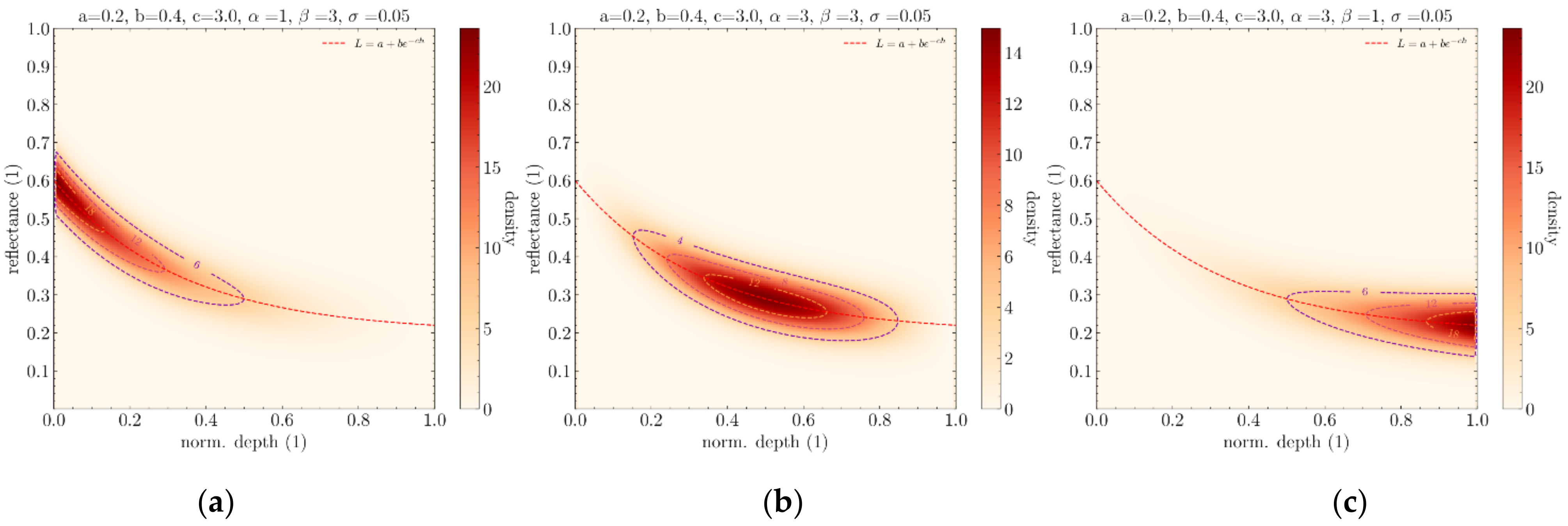
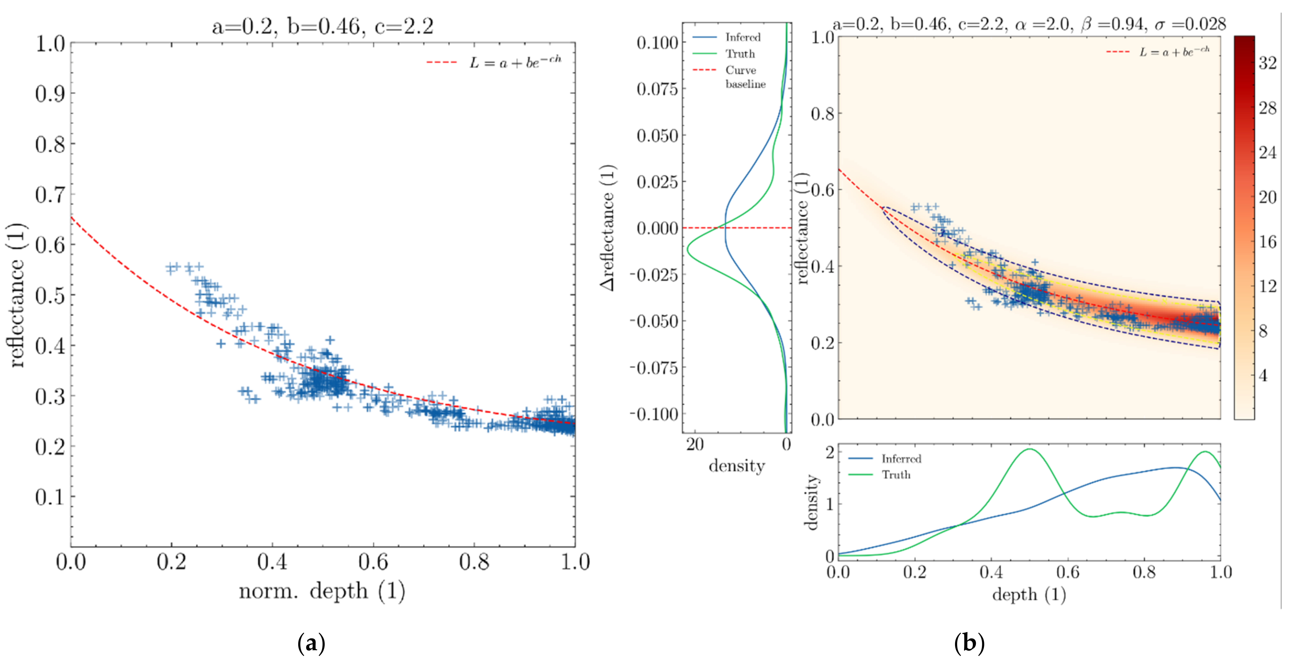
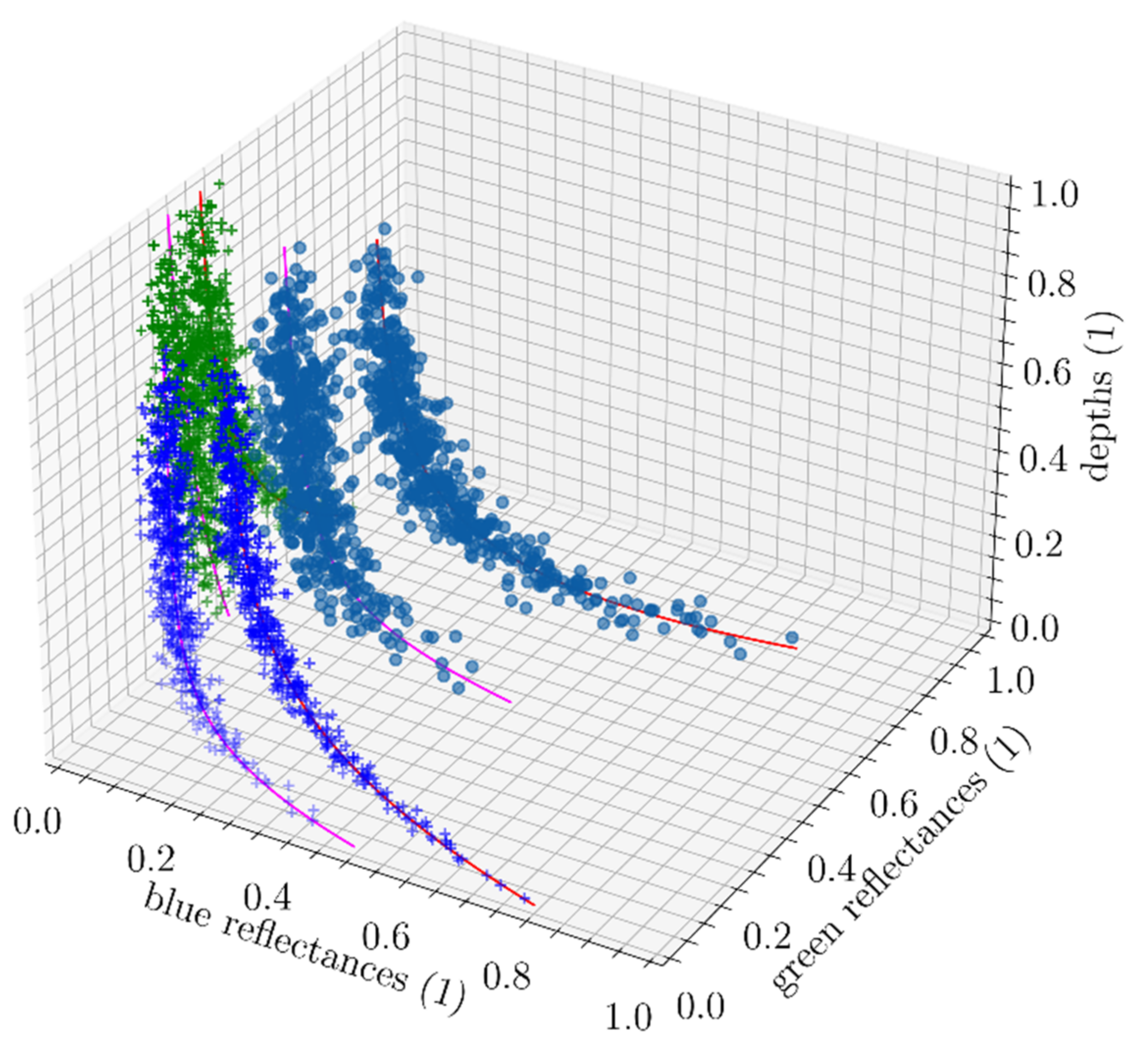
4.2. Single Spectrum Beta-Normal-Polynomial-Exponential Distribution

Instead of restricting the main equation and its domain (by fixing some arbitrary parameters or supposing a correlation between them), some statistical parameters are judiciously added to increase flexibility and ease of use in the context of noisy measurements. In WCPE, the main objects used when building a bathymetry model are probabilistic distributions with support in the depth-reflectance(s) space, centred around curves derived from Lyzenga’s equations. Those distributions are given substance (a probabilistic hull) in this space thanks to a dispersion parameter accounting for noise on reflectance values, as well as a variable following a beta distribution constraining the domain of validity of the object over an arbitrary range of depths. From here onward, such distributions will be referred to as Beta-Normal-Polynomial-Exponential distributions, or BNPs for convenience’s sake.

Let us first define BNPs in the case of a single spectral band like the title of this section suggests.

4.2.1. Definition

The notation for a $BNP$ distribution $D$ with parameterisation $a\in \left[0, 1\right], b\in \left[0, 1\right], c\in {ℝ}^{+}, \alpha \in \left[0, 1\right], \beta \in \left[0, 1\right], \sigma \in {ℝ}^{+}$ is:

$$D ~ BNP\left(a,b,c,\alpha ,\beta ,\sigma \right)$$

(3)

$a$, $b$ and $c$ refer to the parameters of the simplified Lyzenga’s Equation (2), α and β scalars correspond to the parameters of the underlying beta distribution, and σ is a scalar that corresponds to a dispersion parameter along the axis of reflectances. In the case of a single spectrum being used, this distribution has support in the space of the product of depths by reflectances, [0, 1] × [0, 1]. Its probability density function (PDF) is defined as follows:

$$\begin{array}{ll}{f}_{D\left(h,L,a,b,c,c,\alpha ,\beta ,\sigma \right)}& =f_{Beta}\left(h,\alpha ,\beta \right)f_{Normal}\left(L,a+b e^{-ch},\sigma \right),\\ & h\in \left[0, 1\right],L\in \left[0, 1\right]\end{array}$$

(4)

with h the input depth normalised and L the input reflectance observed. $f_{Beta}$ is the PDF of the beta distribution and $f_{Normal}$ is the PDF of the normal distribution.

The three following Figure 10, Figure 11 and Figure 12 exhibit a few possible instances of BNPs.

4.2.2. Relations between BNP Distributions and In Situ Depth Reflectances

The motivation behind BNP distributions is that they can help us formally describe clouds of points in the depth-reflectance space and allow us to use standard statistical tools to help infer underlying parameters, such as parameters from Lyzenga’s equation.

The following figure shows a small dataset of depth-reflectance points along with a snapshot of the satellite image and ENC they were taken from. This location is used as example because the area is rather uniform (mostly sandy bottom, low turbidity), which makes it easy to create bathymetry models.

Figure 13 shows that curves from Lyzenga’s equation emerge naturally from simple data samples. Here, this dataset presumably contains only one water- profile which makes the curve quite apparent. Because real in situ data samples do not perfectly follow those equations and are affected by noise, adding a dispersion parameter makes sense. The addition of this dispersion parameter means that instead of studying mere curves we study densities in the depth-reflectance space. In the case of BNP distributions, the dispersion of the reflectance of samples relative to the curve was supposed to follow a normal distribution because it is the standard distribution adopted when modelling unspecific noises.

Another important piece of information that can be gathered from Figure 4 is that samples from a water column profile may be more or less concentrated at certain depths. In certain regions this can be even more marked. Some types of seafloor algae, for instance, may require to be covered by a certain amount of water to thrive, leading to the existence of a water-column profile specific to a certain depth range only.

Figure 14 is a scatter plot of some toy data (generated from two BNPs) showing what a region containing two very distinct profiles spanning different depth ranges may look like. Many statistical distributions can be used to model the localisation of water profiles. In BNP distributions, a beta distribution is used for that purpose. The main advantage of beta distributions is that they are understood quite well. Their PDF is easily computed, and they only require two parameters to describe very diverse and relevant possible distributions. The only inconvenience is that they only work in a constrained interval, so the depth range studied needs to be upper bounded by some arbitrary value to allow normalisation (ideally within [0, 1]). This is not much of a problem because deriving bathymetry from satellite images is not possible with depths superior to 30 m anyway.

4.2.3. BNP Parameter Regression

Let us consider a dataset of n depth-reflectance samples $\left(hi,Li\right)\in \left[0, 1\right],i\in \left[0,n\right]$. We infer that the parameters of a BNP distribution from those samples is completed in a three-step manner.

The first step consists of regressing parameters a, b and c from Lyzenga’s equation. The simplest way to achieve it is to use the least-square method. This leads to the following minimisation problem:

$$\Delta L={{\displaystyle \sum }}_i^n{\left(L_i-\left(a+b{e}^{-c{h}_i}\right)\right)}^2$$

(5)

Unfortunately, unlike for simpler equations such as $y=b{e}^{-cx}$ there is no analytical formula to compute it, so an optimisation algorithm must be used. WCPE internally uses an implementation of the L-BFGS-B algorithm described here [8,9,10]. At the end of this step, parameters a, b, and c should have been obtained.

The second step consists of computing the dispersion parameter $\sigma$ from vector $L_i-\left(a+b{e}^{-c{h}_i}\right)$. This intuitively corresponds to the amount of spreading of the data samples around the curve whose equation $L\left(h\right)=a+b{e}^{-ch}$ was obtained in the first step.

The third step consists of inferring parameters α and β of the underlying beta distribution. This can be completed independently of steps 1 and 2 as it only requires computing the parameters of a beta distribution using the depths of the training samples. Those can be computed using the method of moments [11], among other methods.

Figure 15 shows the resulting BNP after inferring parameters using the real in situ data introduced in Figure 13. Notice how the probability density of the beta distribution roughly follows that of the true depth distribution of the data samples. Although the distribution appears consistent with the data, the inferred depth distribution does not quite capture the fact that it is bimodal (green curve). This is a limitation due to using only a single BNP to approximate this dataset when two might have made more sense. This kind of limitation will be lifted after introducing the concept of BNP mixtures in a later section.

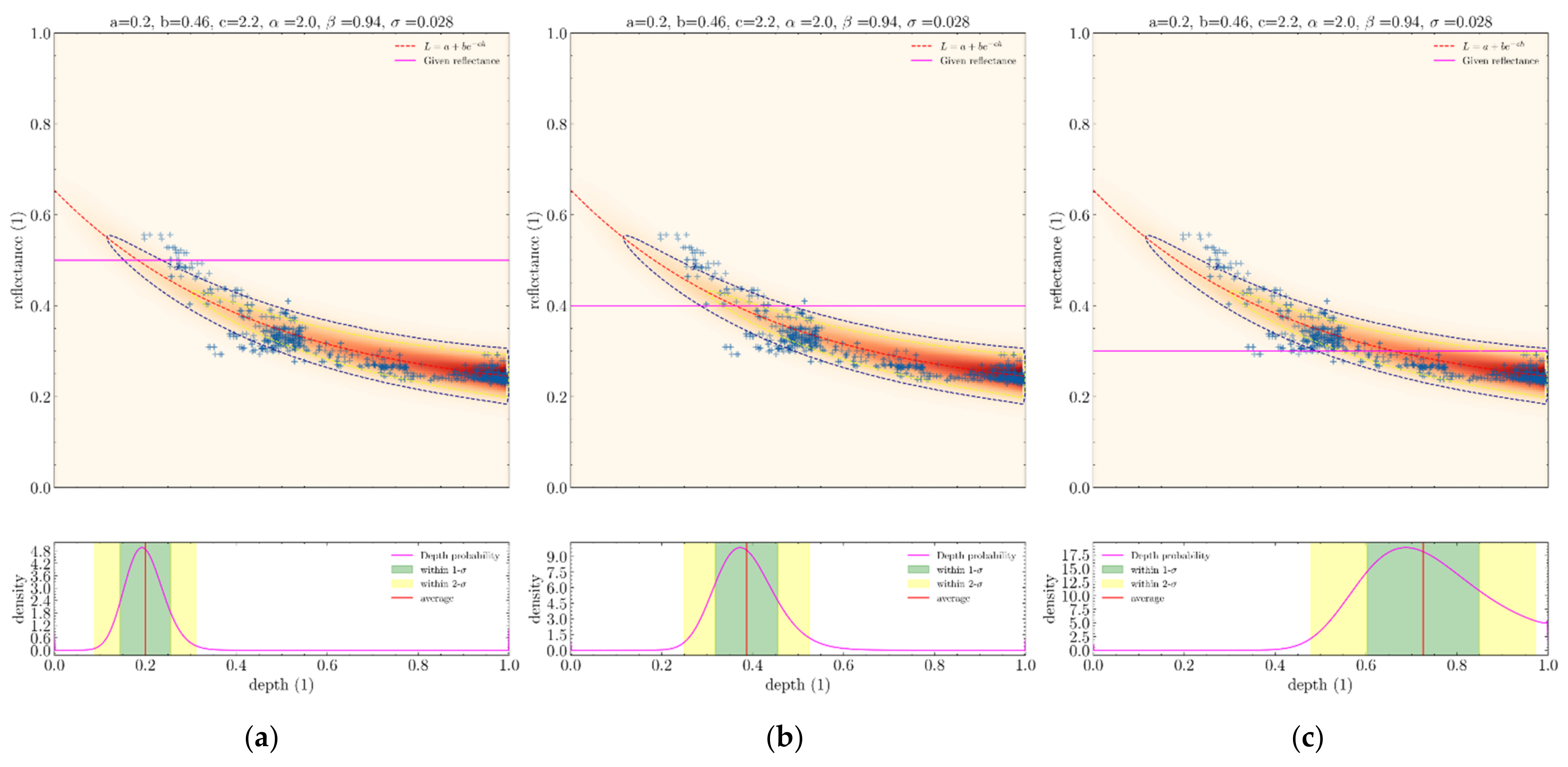
4.2.4. Depth Inference

Figure 16 shows how depths are inferred from some given reflectance values using the BNP distribution inferred in the previous section. For a given distribution D, BNP and reflectance L, the average depth for a given reflectance L is equivalent to the expectation of D.

Figure 16. Inferring depth for a given input reflectance (horizontal magenta line) for a single BNP distribution trained on a few sample points (blue crosses). Three cases shown here. (a) high reflectance. (b) average reflectance. (c) low reflectance. The range of possible depth values for the given reflectance sample can be seen below in the form of an histogram with uncertainty ranges detailed.

Figure 16. Inferring depth for a given input reflectance (horizontal magenta line) for a single BNP distribution trained on a few sample points (blue crosses). Three cases shown here. (a) high reflectance. (b) average reflectance. (c) low reflectance. The range of possible depth values for the given reflectance sample can be seen below in the form of an histogram with uncertainty ranges detailed.

$$h_{\mu }\left(L\right)={{\displaystyle \int }}_0^{1}h{f}_D\left(h,L\right).\delta h$$

(6)

For a given reflectance L, the standard deviation h_σ associated to this depth is simply the square root of the variance of D.

$$h_{\sigma }\left(L\right)=({{\displaystyle \int }}_0^1{h}^2{f}_D\left(h, L\right).\delta h-h\left(L\right){)}^{-2}$$

(7)

In practice, those integrals do not have an analytic form allowing them to be computed exactly. Therefore, they must be approximated using finite sampling.

$$h_{\mu }\left(L\right)\approx \frac{{{\displaystyle \sum }}_0^1{h}_i{f}_D\left(h_i,L\right)}{{{\displaystyle \sum }}_0^n{f}_D\left(h_i\right)}, h\in {\left[0, 1\right]}^n, n\in {\mathbb{N}}^{\star }$$

(8)

Sampling allows to compute not only the average depth and standard deviation, but also any statistical moment (kurtosis, etc.), as well as other interesting measures such as median, quantiles, and so on. The only limit is the number of samplings one is willing to perform. This number dictates the computation time and the precision of the statistical parameter inferred. A high sampling number makes the process slow but precise. Conversely, a low sampling number makes it fast but inaccurate. Finding a good balance between those two depends on the application one has in mind. If inference speed is a major concern, an optimisation could consist of pre-computing relevant parameters for all possible reflectances into an LUT that can be accessed later. This is implemented in WCPE in a way that makes full usage of parallelism in modern machines, considerably reducing the time required to build up such LUT.

Lastly, take note that in Figure 6 the lower the reflectance, the larger the imprecision on the depth inferred which intuitively makes sense since lower reflectances tend to correspond to those of the open ocean, where depth is harder to retrieve.

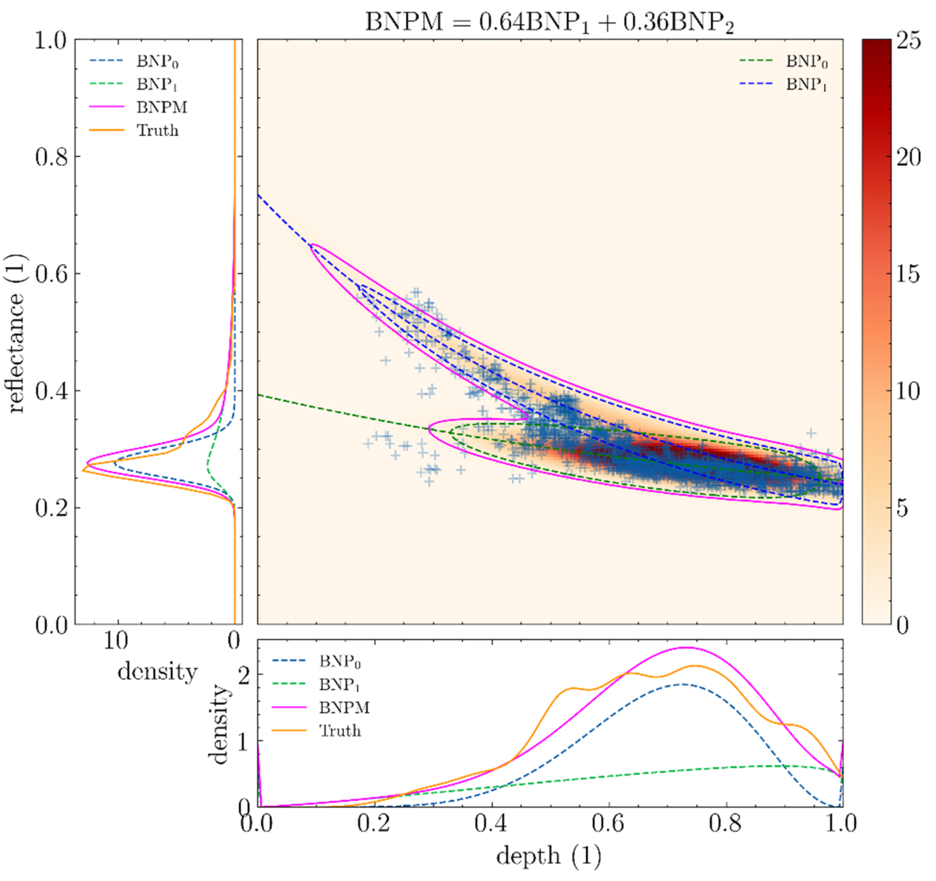
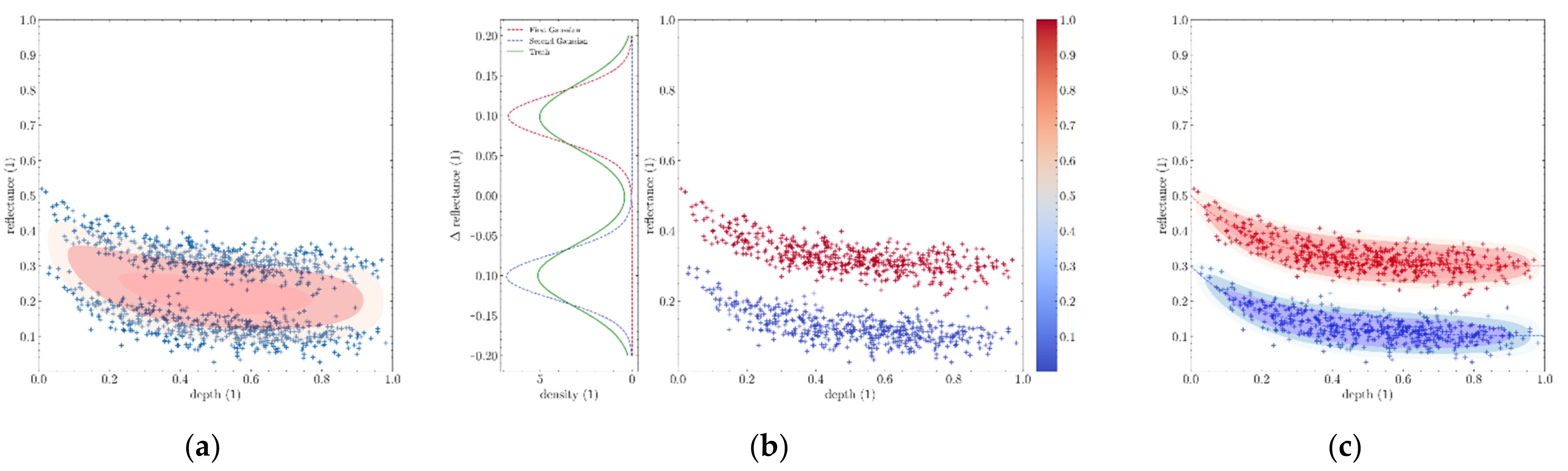
4.3. Single-Spectrum BNP Mixtures

BNP distribution is a convincing tool used to partition the depth-reflectance space, but it is too simplistic when taken individually to model the harder datasets available. To take into account situations such as the one encountered in Figure 5, more than one BNP must be used. In WCPE, this is completed with BNP mixtures.

4.3.1. Definition

A BNP mixture is a distribution that is itself a weighted combination of BNP distributions. The notation for an $n\in {\mathbb{N}}^{\star }$ components BNP mixture $M$ with components $D_i\in \left[0,n\right]~ BNP$ and weights $W_i\in {\left[0, 1\right]}^n, {{\displaystyle \sum }}_i^n{W}_i=1$ is

$$M ~ BNPM\left(D, W\right)$$

(9)

Its PDF is defined as:

$$f_M\left(h,L,D,W\right)={{\displaystyle \sum }}_i^n{W}_i{f}_{D_i}\left(h, L\right)$$

(10)

with $f_{D_i}$ the PDF of each sub-distribution.

An example of a BNP mixture is shown in Figure 17. The ability to combine various BNPs together allows to model very complex datasets and reduce them to their core descriptive physical features.

4.3.2. BNP Mixture Regression

In WCPE, the way a BNP mixture is regressed using some samples is completed using pure application of the expectation-maximisation (EM) algorithm iteratively until all components have converged. The purpose of this article is not to give a description of the EM algorithm since it is already highly documented in the scientific literature, and it is completely independent of the concept of BNP distributions anyway. Internally, WCPE uses a general mixture solver named pomegranate, https://github.com/jmschrei/pomegranate [12], along with a custom implementation of the BNP distribution (based on Equation (4)).

To illustrate the use of BNP mixtures with real in situ samples, we shall consider the satellite image and ground truth measurements displayed in Figure 18.

Figure 19 shows the result of fitting a BNP mixture on the dataset from the previous Figure 18. The dataset seems to fork in the middle, yet the mixture was able to judiciously cover both branches with a BNP, reducing the error against ground truth density compared to only using one component. However, dealing with very complex datasets requires using mixtures comprising a huge number of BNP distributions. Starting the EM process with all BNP distributions right from the start leads to a very poor result. That is because the initialisation the EM process is the most tedious step to get working, as it requires some starting parameters to be assigned to each sub-distribution. The only easy case when initialising BNP mixtures is when they consist of only one BNP, because then initialisation is essentially the same as regressing the BNP using the dataset independently of the concept of the mixture. For mixtures with multiple BNP distributions, it is not evident how one would assign appropriate a priori parameters to each BNP. This is, after all, the whole purpose of the mixture. A prioris selection is a very active field of research in statistics. For more conventional mixtures (Gaussian mixtures for instance), non-parametric methods such as K-NNs have been known to yield decent priors. In the case of BNP mixtures, starting parameters are much harder to guess because of the non-trivial way they interact within themselves to give BNPs their diverse and complex characteristics.

An elegant way to solve this problem is to start a mixture with a single component, since this is the only case we know how to solve confidently, and then successively update the mixture and split its components into more components whenever it is sensible, until the resulting mixture explains the training dataset well enough. The intuition behind this method is that a cloud of samples may be loosely first approximated by a single BNP distribution, before being further decomposed into smaller and smaller clouds. Taking advantage of the fractal nature of those clouds of samples only requires following the base EM process with occasional splits whenever the EM process gives signs that it is stagnating (low increase in the likelihood score of the mixture).

Many methods are possible when it comes to splitting components. Two kinds of splits are implemented in WCPE:

• Splits along the reflectance axis, using the distribution of offsets of training samples relative to the curve of the BNP considered.
• Splits along the depth’s axis, using the distribution of depths of the training samples.

It is to be noted that during each of those splits the totality of the training samples points are considered but weighted accordingly to their contribution to the BNP being split. For the split along reflectances, we train a mixture of two Gaussian distributions on samples offset to the curve. For the split along depths, we use a mixture of two Beta distributions. In each case, we obtain two components. The weights of the samples according to each component are then used to fit two BNPs, which are then included into a small BNP mixture that is trained for a few iterations. Depending on how much better the likelihood of the resulting mixture is compared to that of the original BNP component, we either:

• Keep the original BNP. No split occurs.
• Use the BNP mixture resulting from the split along the reflectance axis.
• Use the BNP mixture resulting from the split along the depths axis.

An even more elegant way to split that was considered during the conception and implementation of WCPE was to directly train a single 2-components BNP mixture using both depth and reflectance features, but the results were not very encouraging. This has either to do with a poor implementation or with the fact that non-parametric methods for estimating priors just do not work very well with BNP mixtures. More work is required to determine which it is the real cause.

Figure 20 is an example of splitting in two a BNP distribution along its depth axis using a 2-component β-distribution mixture. The samples of that figure were generated so that a split along depths made the most sense.

Similarly, Figure 21 is an example of splitting a BNP distribution in two along the reflectance axis, this time using a Gaussian mixture on the offset of the samples to the curve (note the difference in scale between the density plot and the scatter plot in the middle image).

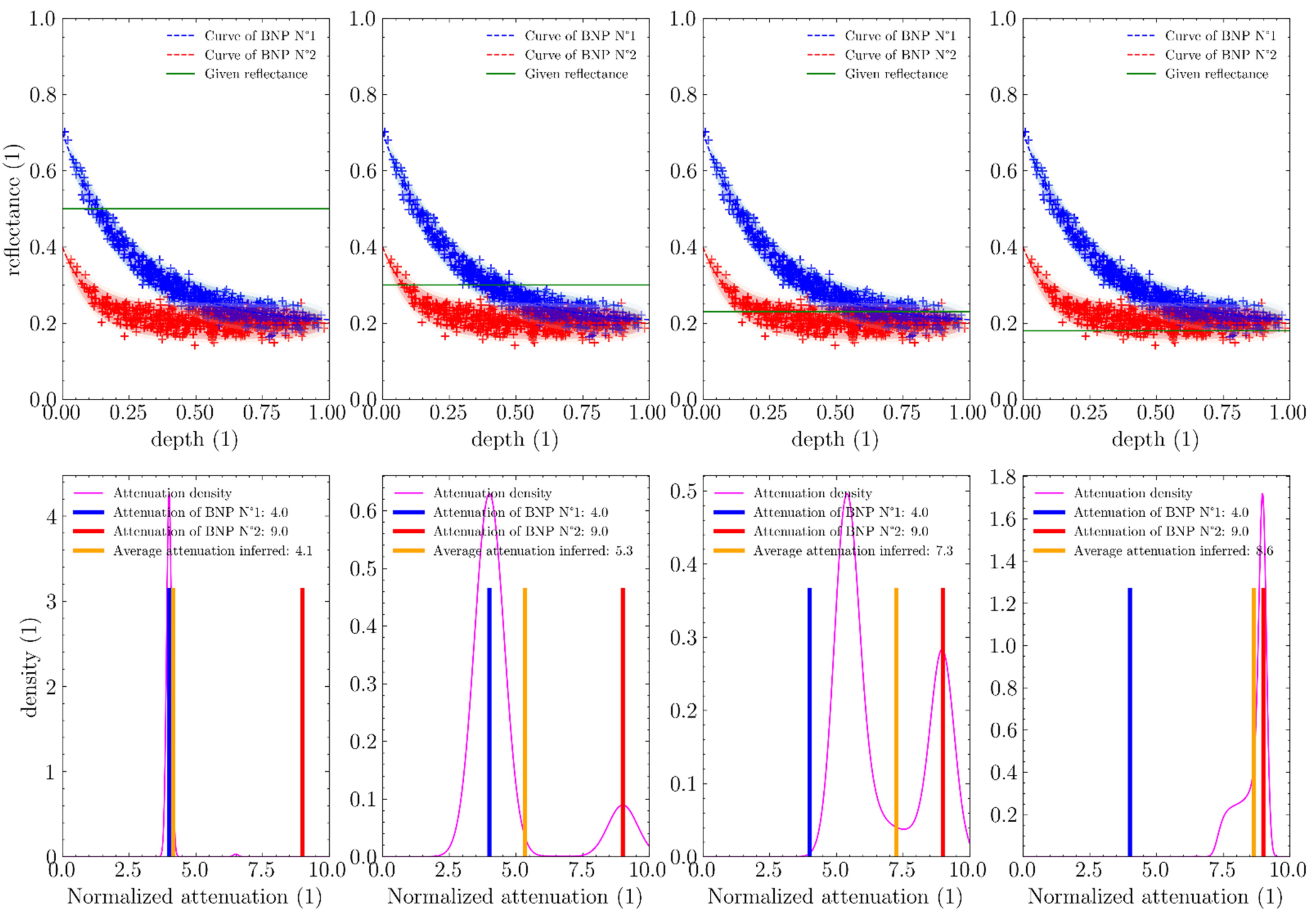
4.3.3. Inferring Depths and Specific Physical Parameters

Depth inference works the same as with a single BNP distribution, except densities are now sampled from the whole mixture using its PDF:

$$h_{\mu }\left(L\right)={{\displaystyle \int }}_0^{1}h{f}_{BNPM}\left(h,L\right).\delta h$$

(11)

One thing we can do now that we could not do before with only one BNP is to infer some arbitrary parameters related to the BNPs of a mixture. For instance, one might be interested in computing the attenuation coefficient for a given reflectance. One may even want to extract some arbitrary attributes of BNPs, computed from their parameters. Inferring those attributes for the whole mixture is a bit more convoluted than doing it with depths as it warrants an additional step. Let us consider a mixture M composed of $n\in {\mathbb{N}}^{\star }$ components $D_{i\in \left[0,n\right]}~BNP$ with weights $W_i, {{\displaystyle \sum }}_i^n{W}_i=1$, each with respective parameterisation $a_i, b_i, c_i, {\alpha }_i, {\beta }_i, {\sigma }_i$. Let us consider an attribute x_i computed for each D_i using a function g:

$$x_i=g\left(a_i, b_i, c_i, {\alpha }_i, {\beta }_i,{\sigma }_i\right)$$

(12)

Or more succinctly:

$$x_i=g\left(D_i\right)$$

(13)

Let us first define $x_{h,L}$ as the weighted average of all attributes x_i at depth h and reflectance L with respect to the density of their respective BNP $D_i$ found there.

$$x_{h,L}={{\displaystyle \sum }}_i^n{x}_i{W}_i{f}_{D_i}\left(h,L\right)$$

(14)

The average value for attribute x is then given by:

$$\begin{gathered} x_{\mu }\left(L\right)={{\displaystyle \int }}_0^1{x}_{h,L}{f}_M\left(h,L\right).\delta h \\ ={{\displaystyle \int }}_0^1\left({{\displaystyle \sum }}_i^n{x}_i{W}_i{f}_{D_i}\left(h,L\right)\right)f_M\left(h,L\right).\delta h \\ ={{\displaystyle \int }}_0^1({{\displaystyle \sum }}_i^{n}g\left(D_i\right)W_i{f}_{D_i}\left(h,L\right))f_M\left(h,L\right).\delta h \end{gathered}$$

Similar to the formula we used to compute the average depth. Extracting other statistical parameters is completed in a similar manner, by first computing x_h,L and then replicating the same step as when deriving depth statistics. Sampling also works the same, and LUT can also be computed for faster inference of those parameters.

Here, a few specific function g that may be of interest to some readers and that can be computed using this method are presented:

-

$g\left(D_i\right)=a_i$ → deep-sea reflectance.

-

$g\left(D_i\right)=a_i+b_i$ → seafloor reflectance.

-

$g\left(D_i\right)=c_i/S$ with $S$ a coefficient dependent on the scene geometry → attenuation coefficient.

-

$g\left(D_i\right)=\min (0, \frac{\ln \left(\frac{b}{dL}\right)}{c})$ with $dL$ the minimum discriminating reflectance quanta (dependent on the signal-noise ratio of the instrument used) → cut-off depth/depth of penetration.

Figure 22 shows how WCPE infers the value of a parameter (here the attenuation coefficient) for a given reflectance in a mixture where two components have different values for this parameter. In non-ambiguous cases (first and last pictures), WCPE correctly guesses the correct value. In ambiguous cases (when the two components frequently overlap for the given reflectance), the average value of the parameter is neither that of the first nor the second component, but a value in between, which is erroneous. Fortunately, the standard deviation for such cases can be shown to be quite large (the magenta density curve is wide), which gives a clear indication that the value is not very accurate.

4.4. Multi-Spectral BNP Mixtures

Until now, only single-spectral BNP mixtures were considered. However, using a single spectrum to derive bathymetry usually does not give very accurate results. This is because some water-column profiles may share similar reflectances but have widely different depth ranges. The use of an extra spectral band was adopted very early in the infancy of SDB to increase the ability of bathymetry models to be able to resolve bad cases. Incorporating new spectral bands in WCPE is completed effortlessly by changing the definition of the BNP distribution. The only difference is that the distribution is now multivariate with respect to parameters a, b, c, and σ. Given n spectral bands, the definition of a multi-spectral distribution BNP is now:

$$D~BNPM\left(a,b,c,\alpha ,\beta ,\sigma \right), a\in {\left[0, 1\right]}^n, b\in {\left[0, 1\right]}^n, c\in {ℝ}_{+}^n, \alpha \in \left[0, 1\right],\beta \in \left[0, 1\right],\sigma \in {ℝ}_{+}^n$$

(15)

Its PDF becomes:

$$\begin{gathered} f_D\left(h,L,a,b,c,\alpha ,\beta ,\sigma \right)=f_{Beta}\left(h,\alpha ,\beta \right){{\displaystyle \prod }}_i^n{f}_{Normal}\left(L_i, a_i+b_i{e}^{-c_{i}h},{\sigma }_i\right) \\ =f_{Beta}\left(h,\alpha ,\beta \right)f_{Normal}\left(L, a+b{e}^{-ch}, \sigma \right), h\in \left[0, 1\right], L\in {\left[0, 1\right]}^n \end{gathered}$$

Figure 23 shows an instance of a two-spectrum BNP mixture with two components (red and magenta curves). A cloud of sample points is visible in lighter blue. Green points are the projection of the sample points onto the depth-green plane and blue points are the projection of the sample points onto the depth-blue plane. Note that those plane projections are essentially the same to the depth-reflectance plots regularly shown in previous sections. We can recognise the typical exponentially decreasing clouds of points encountered earlier. Multispectral BNP mixtures operate exactly like their single spectral counterparts, except that they are more effective at distinguishing samples, thus, providing better depth assessments in general. The 3D density hulls of the BNP in this mixture are not provided because they would make the plot hard to read.

4.5. Evolution of WCPE

4.5.1. Handling of Ambiguous Cases

Ambiguous cases arise when reflectance alone cannot help to distinguish between two data points belonging to two different water-column profiles. When such conflict exists, they are easily detected by WCPE because they will increase the standard deviation computed from the density profile as shown in the depth inference section. Separating such cases cannot be completed using reflectances alone, so extra information must be provided. There is only one type of information we did not consider so far, and which does not require using other data sources, that is the textural content found within satellite images, i.e., how pixels are distributed spatially. The idea is to train a pure machine learning algorithm to classify an image into two or more classes to be able to train several WCPE models on each separate instance. This method may not solve all ambiguous cases by using textures alone, but it may help.

Rocky features can be hard to distinguish from a deep-sea background because they exhibit a similarly low reflectance profile. However, rocks can be visually distinguished from the deep sea in satellite images, especially when they are clear-cut whereas deep-sea areas tend to be broad and smooth.

Figure 24 shows how to incorporate the ML component allowing separation of ill cases. The first step consists of training a WCPE model the usual way. Then, using this model, we compute an indicator of how confident it is in the resulting depth for every reflectance in the input raster (e.g., standard deviation). This indicator is then used to split the training raster into the classes that need to be distinguished to raise WCPE’s confidence level. A generic neural net with convolution layers, preferably a UNET, is then trained using those classes to make a model M that can be applied to any image similar to the input raster. This model M is used on the input raster and the inferred classes are used to extract their corresponding sets of reflectance values. Finally, a WCPE model is trained on each resulting reflectance set, which should now be devoid of ambiguous cases.

The way to infer depth now requires applying a trained model M on the input raster, then identification of each appropriate WCPE model on the subclasses, before merging the results into the final bathymetry raster.

4.5.2. Deriving Depth in Uncharted Locations

The major limitation of WCPE is that it requires a lot of data for initial training. Such data is available around the world in the few locations that have been adequately surveyed, but most coastal regions remain uncharted (the reason that SDB is required in the first place).

To solve this problem, we briefly describe how to modify the available data to create new sets specifically tailored to nearby AOIs and which can then be propagated from near to far over large regions.

Given a few locations where both reflectances and in situ depths are available, the process is as follows:

• An adequacy score is computed between each raster from charted locations and the raster for which we want to infer new depths.
• Adequacy scores are used with a function that associates a weight to each of them, the total amount of weights summing up to 100%.
• Reflectances and depth values are sampled from each charted location and combined given those weights.
• A WCPE model is trained using those values.

This method requires three main components.

The adequacy function must be able to provide an indication of how close two raster images are. One way to do it is to train a multidimensional Gaussian mixture on the reflectances of each input images then compute the Kullback Leibler divergence between them. Because the Kullback Leibler divergence between mixtures of more than one component is (almost always) intractable, it must be approximated [13].

The function associating a weight to each score computed with the adequacy function depends on what criteria is valued. Typical cases include:

• Only selecting the location with the highest adequacy score (akin to argmax).
• Using adequacy scores as is, with just a normalisation process so they sum up to 100 (akin to 1-norm) %.
• Only selecting the n most adequate locations, with n an arbitrary number.

Many tactics may be employed for the sampling function:

• The most basic one consists of randomly selecting available depth-reflectance samples.
• A more accurate one is to compute the likelihood of each available depth-reflectance sample with the mixture trained for the raster of the uncharted region and then resample among all samples using those as weights.

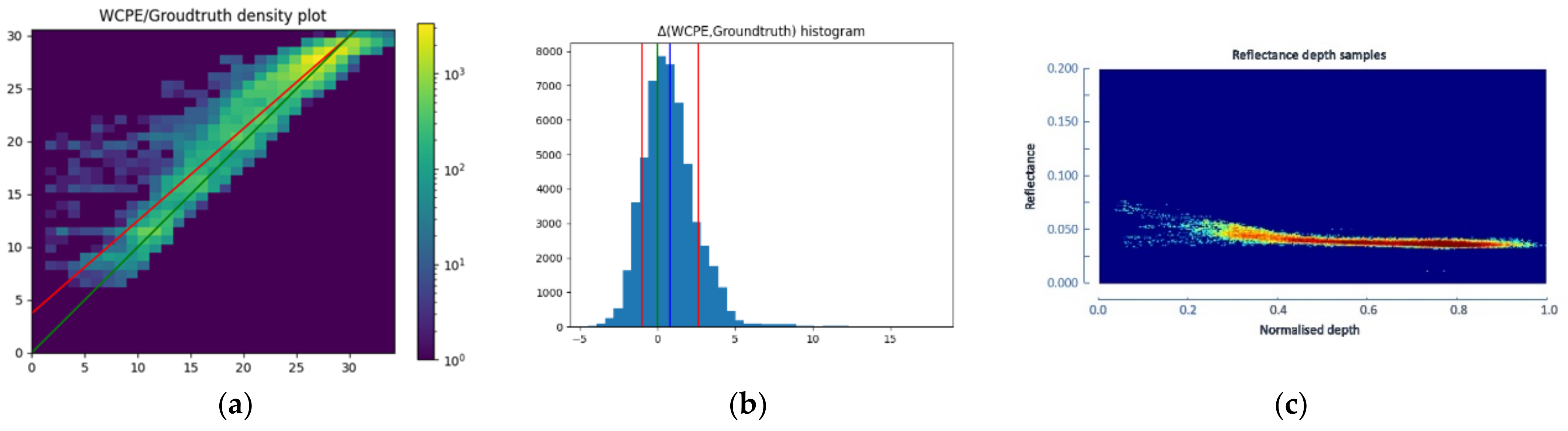
Very few additional assumptions need to be made on top of the postulates behind those, and great care must be employed to avoid falling prey to the trap of over-parametrising any mode.

5. Results

Achieving seafloor coverage with an eye on the Seabed 2030 global ambition.

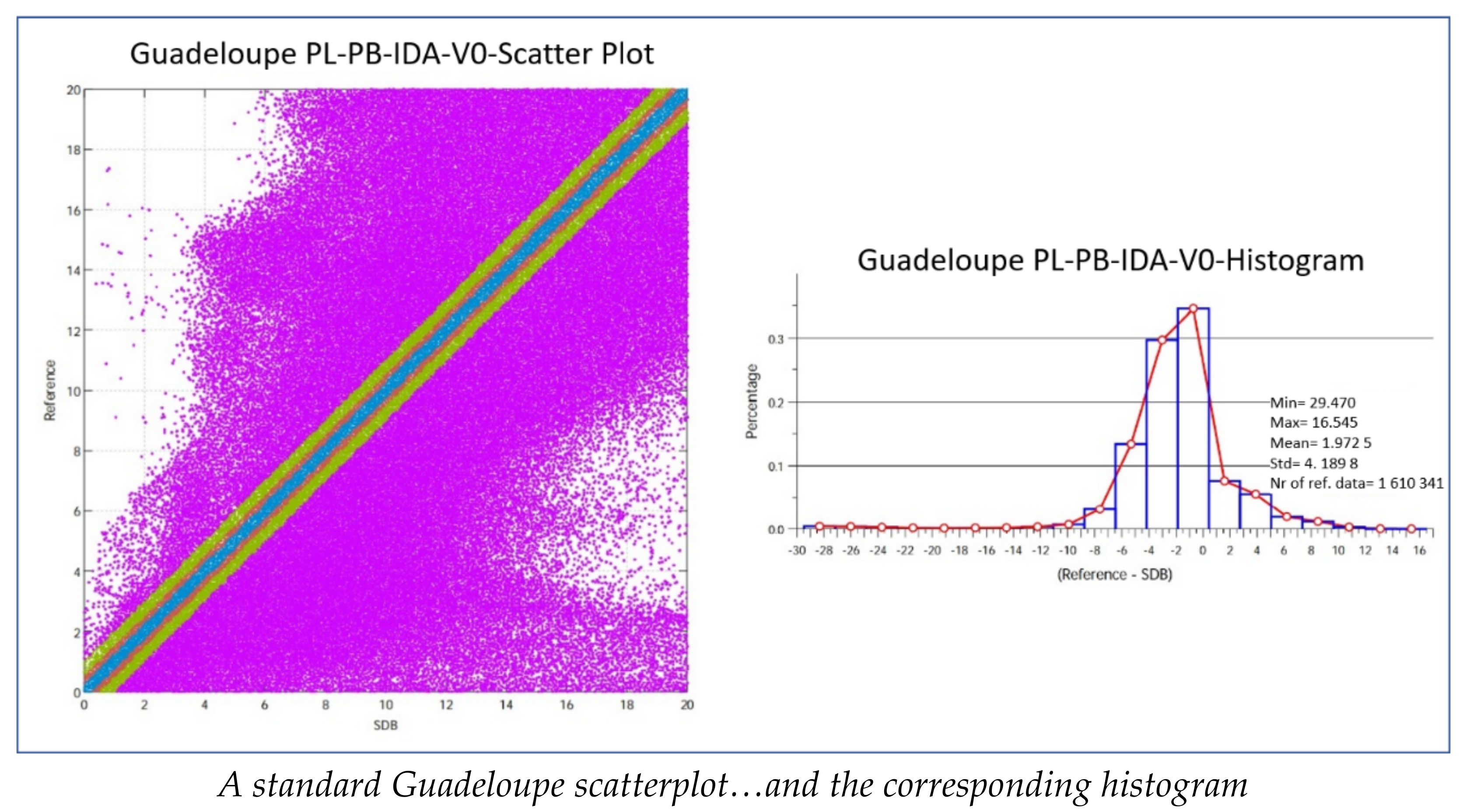
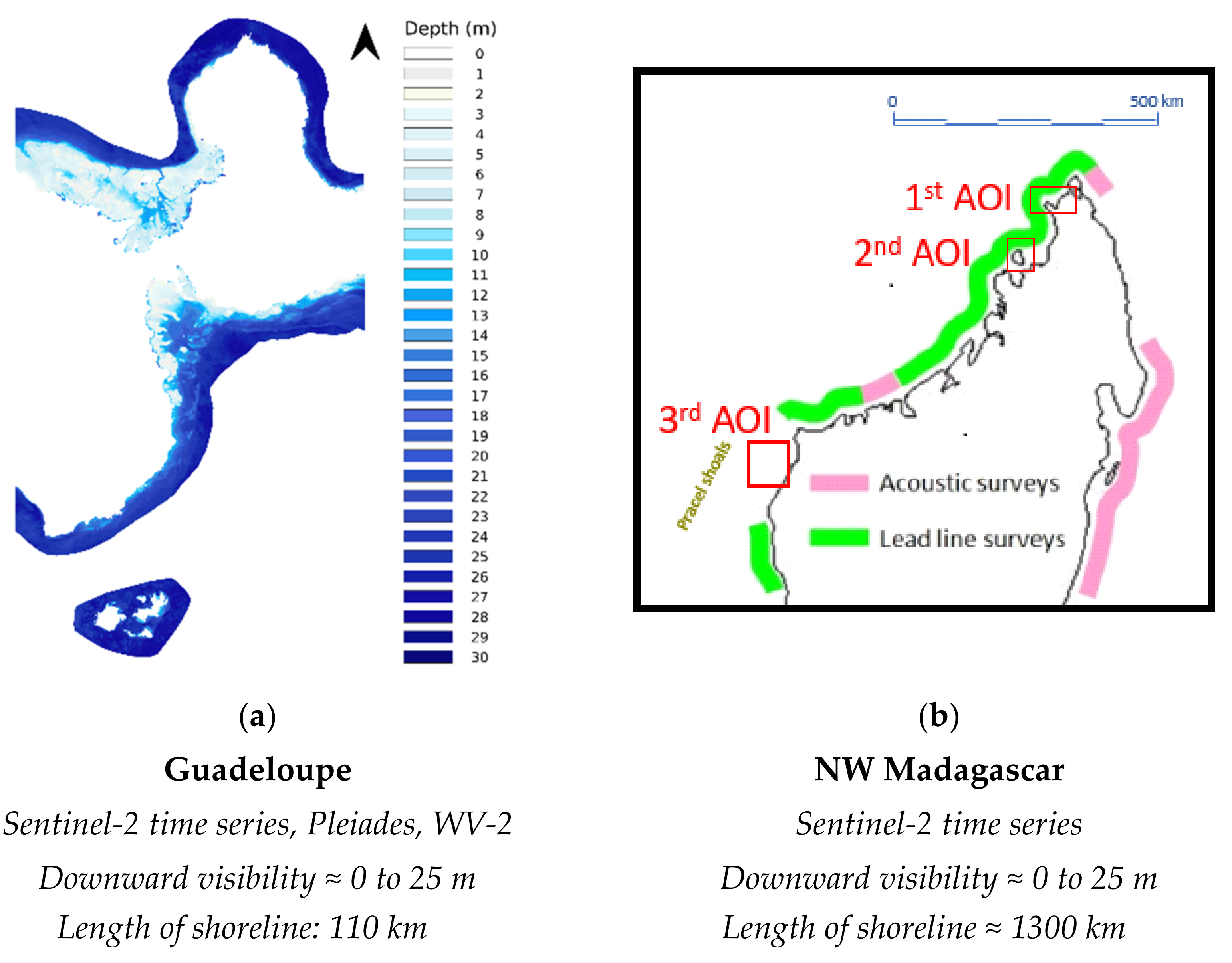
5.1. Guadeloupe First Implementation

Although it includes only 110 km of coastal length, the Guadeloupe AOI comprised all kinds of seafloors characterised by spread-out scatter plots such as the one depicted in Figure 5. Unless split into many subzones, neither of these can yield depths vaguely compliant with the S-44 standards.

To overcome this problem, statistical tools were employed to bridge the differences between the simplistic and rigid nature of the base equations and the great diversity of spectral profiles commonly found in satellite images. The WCPE builds its bathymetry model by using probabilistic curves derived from the base Lyzenga equations matching depth and reflectances. A dispersion variable following a normal distribution was added to account for noise in the range of reflectances observed and a variable following a beta distribution was used to constrain the domain of validity of the object over the range of depths considered.

Although incomplete, the Guadeloupe implementation made important conclusions that influenced all further projects:

• The bathymetric models determined by Sentinel-2 time series are far superior to those yielded by individual VHR images.
• Large areas of interest must be split into homogeneous subzones characterised by similar environments. This requires a preliminary first analysis and sufficient comparisons with ground truths to qualify the subzones.
• There is a need to replay the qualifications, which requires methods and software.

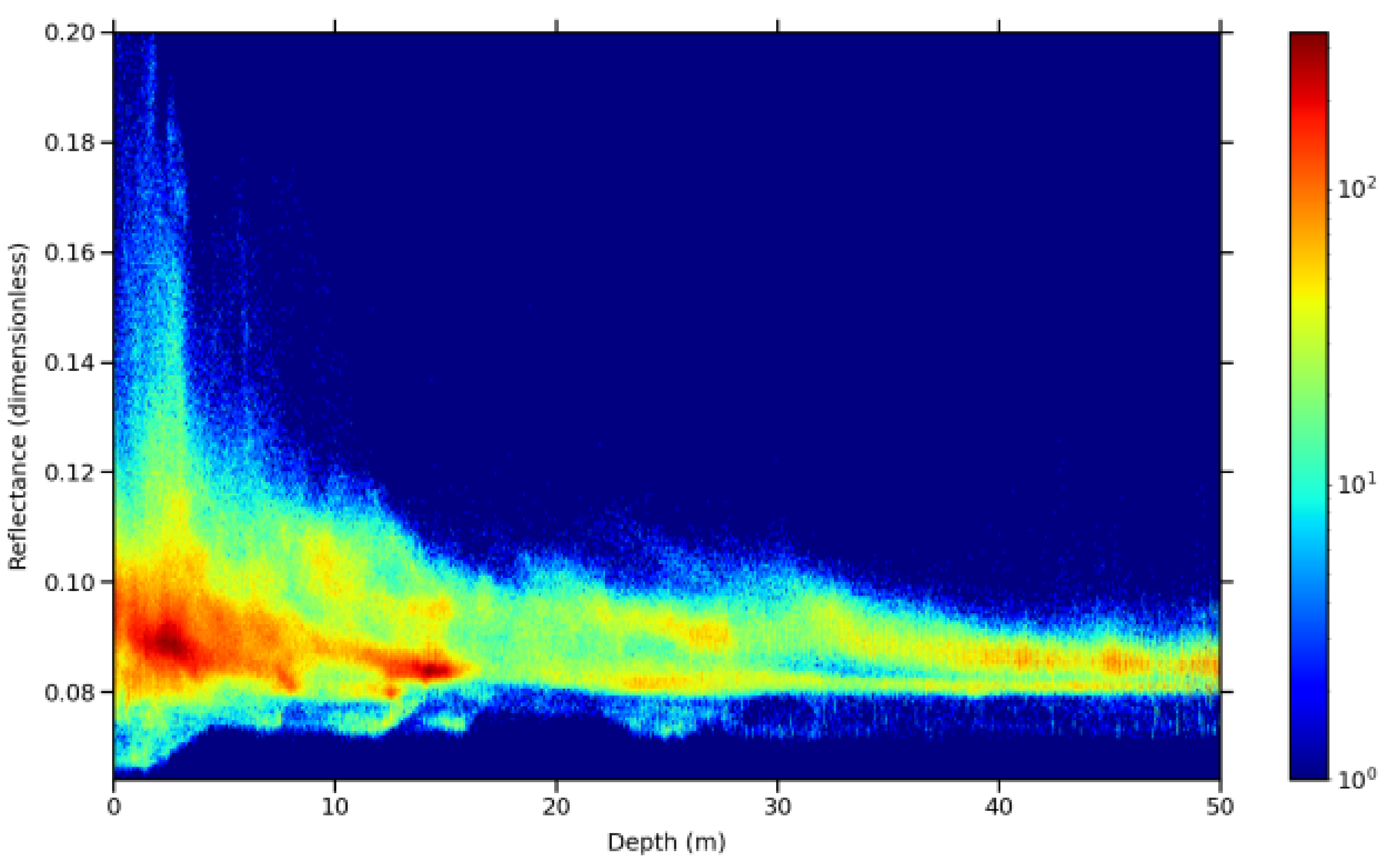
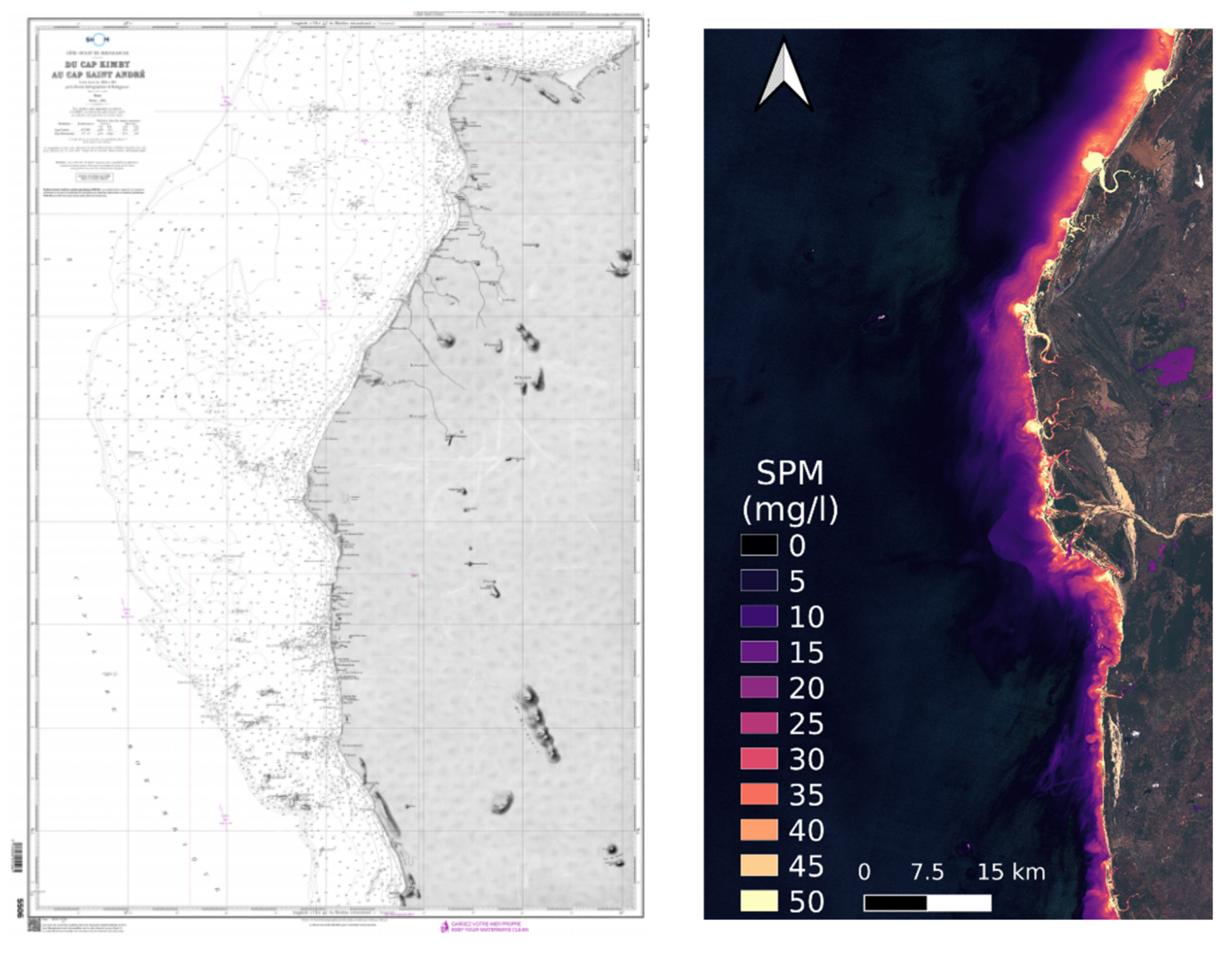
5.2. Madagascar Test Bed: A First Attempt to Survey a Very Large Area

The idea was to demonstrate the WCPE’s capacity to survey large coastal zones meaningful to Seabed 2030 and provide reliable depth figures to populate the GEBCO 100-m grid database. Madagascar is a challenging environment, characterised by a mixture of high turbidity and clear water (see Figure 25), and unsurveyed areas, and seemed appropriate to prove the point.

The experiment consisted of subdividing the zone into three smaller subzones, then linking these subzones using a propagation algorithm to gradually carry out the data inversion based on the starting AOI until the whole area was covered.

The zone was too large to produce a continuous bathymetric model within the required time and budget, but it confirmed WCPE’s ability to develop a valid model with very few external ground truths. It also showed that the method had to be better automatised if one wants to cover the whole world with affordable human resources.

This led to the concept of composite models linked together by morphologic continuity. It further confirmed several important points, both of theorical and practical significance

• Regardless of the merits of the Hydrolight simulation tool, and despite numerous publications, the traditional models of Lee et al. proved insufficient and ill-suited to evolve the SDB methodology. The need to develop an entirely different approach based on statistics was clearly demonstrated by this experiment.
• Once again, the superiority of Sentinel-2 time series over VHR individual images for coastal bathymetry was confirmed, not to mention the value-for-money criteria.
• The need to develop and implement a correction model to mitigate the effects of turbidity became apparent. A way ahead consisting of applying a simple correction to depth depending on the concentration of suspended particular matter was envisaged but could not be completed at this stage.

5.3. A Polynesian Textbook Case: The Tahanea Testbed

To test the WCPE statistic approach against previous successful SDB surveys, the atoll of Tahanea, French Polynesia, was selected for its transparent waters until 25-m depths, manageable turbidity and transients, homogeneous physical environment, and large echosounders surveys to provide ground truths to be compared to.

Tahanea was tested at a time when the Sentinel-2 time series were not available, henc, e WV and Pleiades images were used by WCPE with impressive results. However, a quick investigation performed later showed that the Sentinel-2 time series would have been at least as successful, if not better and certainly cheaper than the VHR commercial images. This was confirmed later in Qatar.

5.3.1. Pleiades Results

Only a few ground truths were necessary to calibrate and train the WCPE model while thousand could have been made available if needed, without bringing any further improvement due to such a homogeneous environment illustrated with Figure 26.

Applied bluntly, the WCPE statistics were crushingly superior to the traditional SDB modelling (IDA) which yielded dubious results as frequently observed with traditional SDB due to suspicious tinkering from analysts determined to optimise their results no matter what. WCPE scatter plots and histograms were not tampered with and, as seen in Figure 27, remain comfortably regular.

With the Pleiades selected images, the WCPE statistics against the traditional Lee et al. SDB model are listed in the following

Table 1. Differences between the WCPE and the traditional SDB model against the Tahanea ground truths (Pleiades).

	WCPE	Traditional SDB Model (IDA)
Std difference	2.74 m	Previous models and IDA poor results were discarded due to analysts’ excessive tampering
Mean difference	0.36 m
Median difference	0.24 m
Absolute difference	2.07 m

:

5.3.2. WorldView Results

The WorldView images procured next have the reputation amongst service providers to be the best. Processed comparatively with WCPE and the traditional Lee et al. SDB model, they yielded the results depicted in Figure 28 and listed in subsequent

Table 2. Differences between the WCPE and the traditional SDB model against the Tahanea ground truths (WorldView).

	WorldView + WCPE	Traditional SDB Model (IDA)
Std difference	1.83 m	3.41 m
Mean difference	0.84	−3.22 m
Absolute difference	1.45 m	3.79 m

.

In such a propitious environment, the WCPE only can reach a level of precision marginally compatible with the 2-m grid DTMs that SDB users tend to require nowadays.

The Tahanea figures qualify the WCPE in its ability to meet the 100 m grid requirement of Seabed 2030, but the question arises about its compatibility with the strict accuracy standards of IHO publication S-44. Can an improved SDB method based on complex statistics, freed from the uncertainties that usually plague the traditional Lee et al. approach, serve effectively as a usable hydrographic tool to ensure the safety of navigation?

It was then decided to proceed a step further and concentrate on the new WCPE statistics paradigm’s capacity to meet the S-44 stringent standards of precision and achieve 100% seafloor coverage and detection of potentially dangerous features. This was tested on the occasion offered by an Oil Supermajor contract looking for safety of navigation in the Qatar coastal waters.

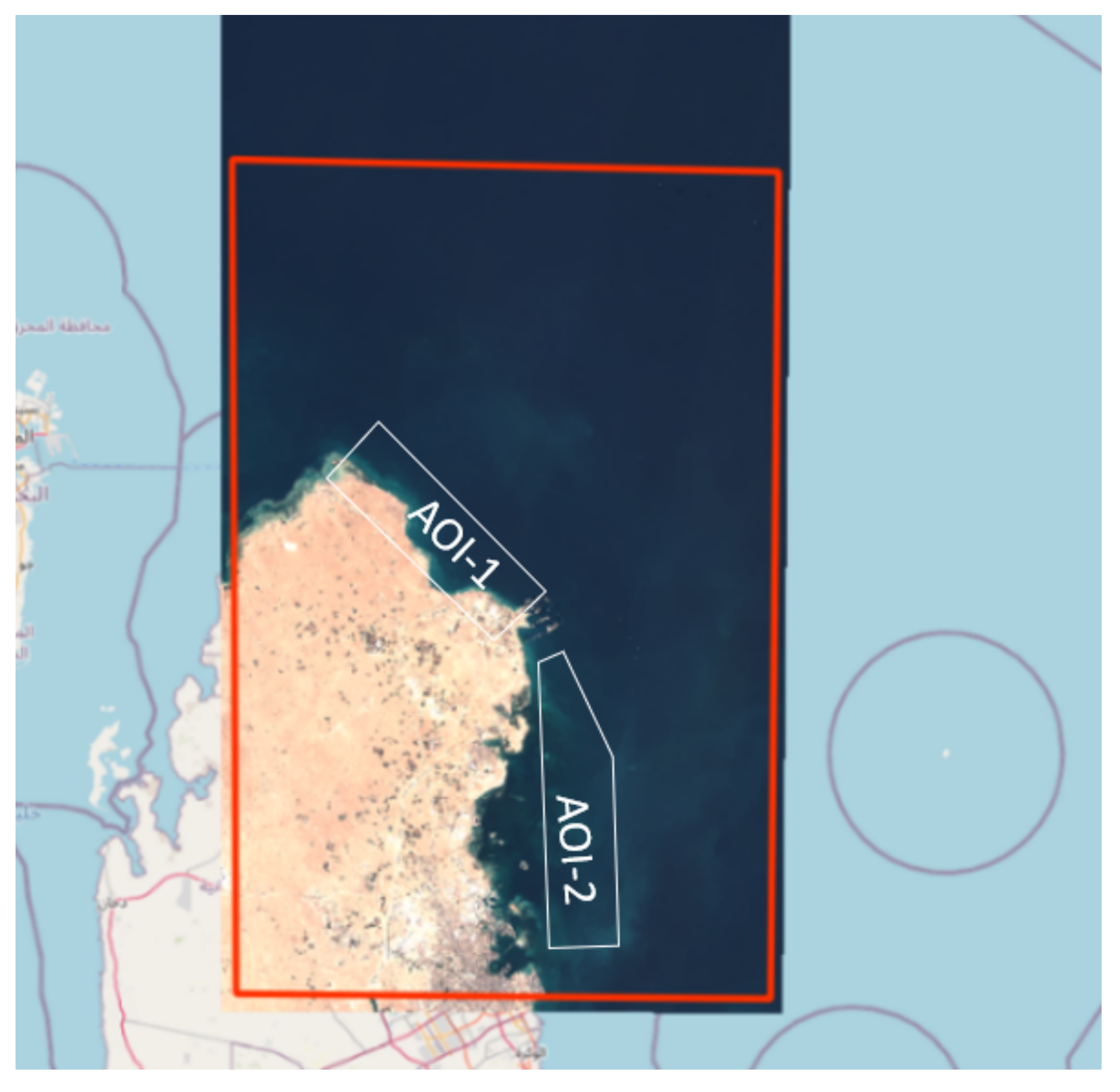
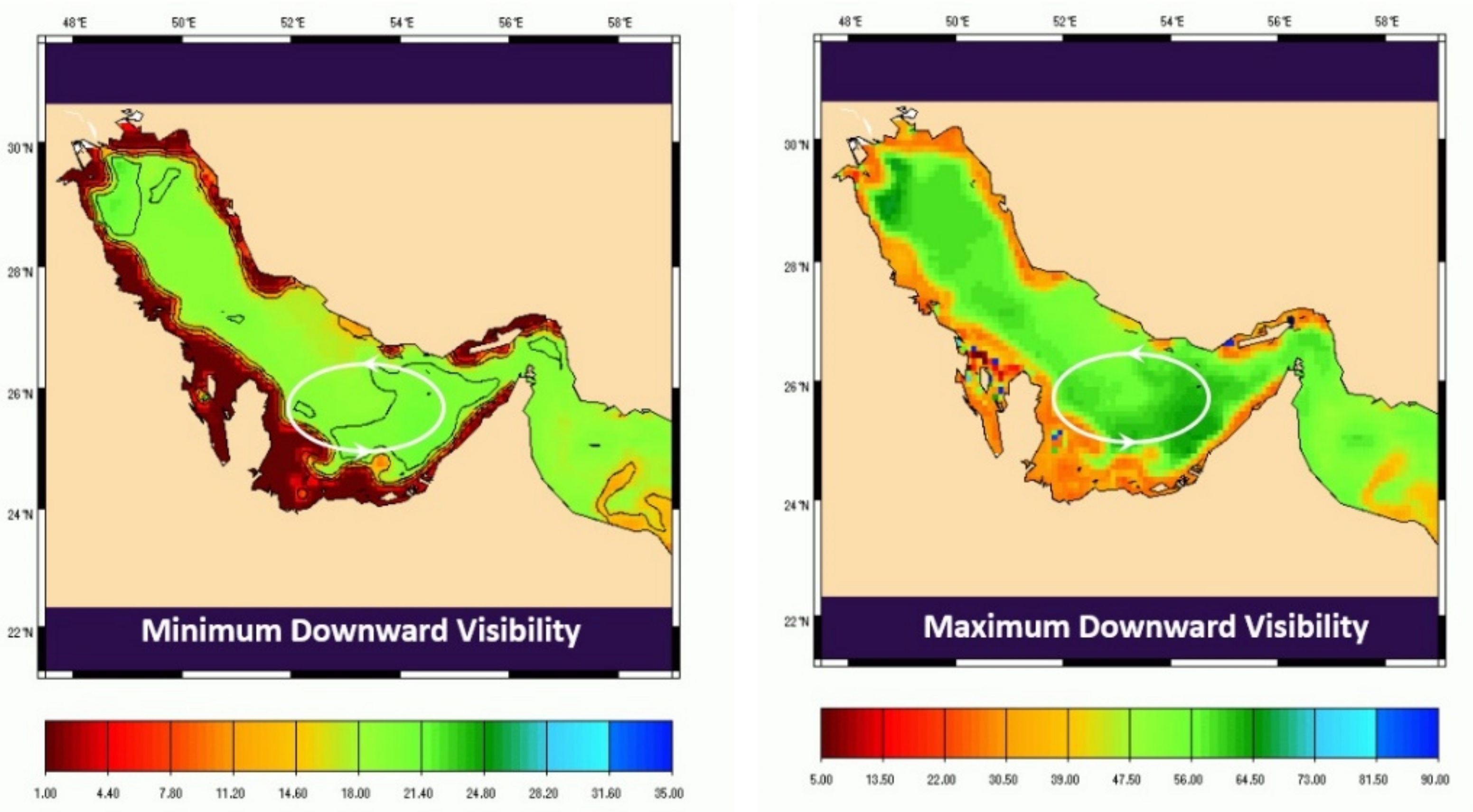
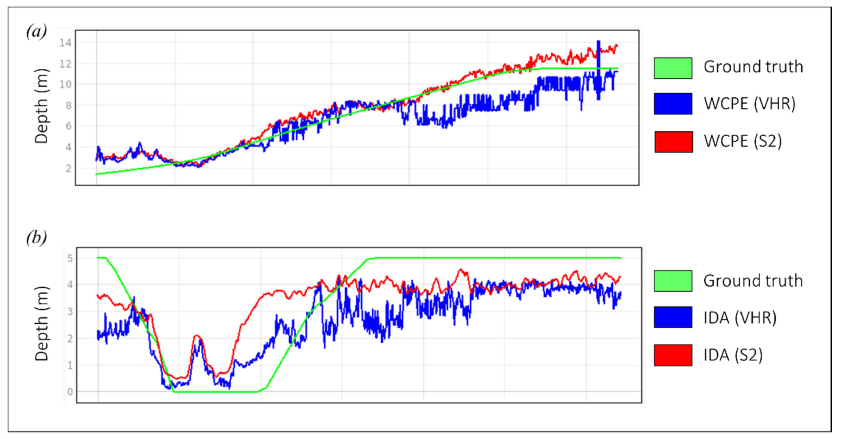
5.4. The Qatar Test Bed

5.4.1. An Experience Centred on Safety of Navigation

The purpose of this study was to determine as exhaustively as possible the performances of satellite-derived bathymetry with regards to the safety of navigation.

The waters of Qatar are characterised by variable turbidity resulting in large differences in downward transparency (Figure 29) encountered in the State’s two tested AOIs (Figure 30).

To this effect, the following combinations were tested on two areas of interest, with special emphasis on the detection of features and potential dangers:

• ARGANS new WCPE statistical model against a traditional Lee et al. RTE model (IDA).
• Selection of high resolution against very-high-resolution images for optimised comparisons.
• Comparison between Sentinel-2 time series against metric to sub-metric commercial images.
• Guided investigation of known charted obstructions with very-high-resolution images (WV, Spot6, Planet scope, Pleiades, etc.).

Special attention was paid to the elimination of biases such as those originating in the use of tidal prediction in the absence of on-site observations. Pseudo-real-time observations were obtained from a tidal model determined by combining simultaneous comparisons between the nearest permanent observatories.

All cartographic sources were examined, including GEBCO’s and the Qatar Municipality Hydrographic Unit’s.

Two 10 m grid bathymetric DTMs were calculated from Sentinel-2 time series and the best available VHR images, using ARGANS WCPE and traditional Lee et al. IDA software. The results were found reasonably close which is normal as they use the same attenuation algorithm, but WCPE associated with the Sentinel-2 time series was deemed more reliable than IDA because it analyses and filters all the image pixels available from a much larger collection of less noisy images.

A 2-m grid DTM was further calculated using the best SPOT-6 pan-sharpened, 1.6 m resolution image, and the results were also compared to the 10 m Sentinel-2 DTM. The 2-m grid DTM was found to be less accurate and less reliable than the 10 m, which is obvious to engineers more aware of the significance of the signal to noise ratio than hydrographers. Not only is the Sen-2 DTM considerably less noisy due to its better SNR but it also suppresses transients and Gaussian biases by stacking and averaging time series, an advantage that no individual VHR images can match.

Despite spending a significant amount of money to procure VHR images, the results are far inferior to those obtained with the public Sentinel-2 DTM.

An optimised composite model comprising the best results from both methods was delivered. As seen in

Table 3. Comparison between precisions offered by WCPE and admiralty charts in Qatar.

	WCPE Composite SDB Model	Admiralty Charts
Precision in the 0–5 m range	Better than 1 m	1.1 m
Precision in the 5–15 m range		1.3 m

and Figure 31, this compares favourably with the accuracies indicated in UKHO’s admiralty charts:

Despite turbidity, an 11-m depth could be guaranteed, but high reflecting seafloors could be seen down to 15 m approximately.

The comparisons between models (WCPE against traditional Lee et al.) and satellite images (VHR against Sern-2) can be summarised by cross sections such as those displayed in Figure 32.

5.4.2. Nautical-Chart-Guided Investigation of Potentially Dangerous Features

A small number of obstructions and wrecks are depicted on the official nautical charts. None of these could be seen, neither on the Sentinel-2 time series nor on the best SPOT-6 pan-sharpened, 1.6 m resolution image.

A further costly effort was attempted by guiding the best WV 0.6 m resolution images on these charted details, but none of these could be detected despite trying to optimise to the extreme of the various tunings.

One must conclude that satellite optical imagery, whatever the resolution and money spent, cannot offer the guarantee required by the publication S-44 for the detection of features. In the absence of sonar searches, the only way to improve this guarantee was by completing the final navigational DTMs with the charted obstructions extracted from separate datafiles by cartographers in a traditional compilation fashion.

6. Discussion

6.1. HR or VHR Images?

Based mainly on signal-to-noise considerations, the results obtained in this study confirm that digital terrain models processed from individual VHR images cannot provide the same level of quality as those calculated with 10 m resolution time series obtained by stacking several carefully selected Sentinel-2 images.

VHR images cannot detect small features with sufficient certainty, and are thus unable to meet the criteria set in the S-44 publication unless completed with dedicated sonar searches, which would make satellite imagery almost irrelevant compared to echosounder surveys. If utilised despite these reserves, VHR models must first be calibrated against more reliable HR models construed with time series to correct their possible biases which can reach several metres, as observed earlier.

This view, which was proven uding repeated observations, is very much resisted by commercial stakeholders and image providers. It should nonetheless be emphasised at technical conferences and seminars in the interest of users.

Despite their systemic weaknesses in the maritime domain, and of course their punishing cost, it should be noted, however, that metric and sub-metric resolution imagery and DTMs are well suited to intertidal zone applications, coastal erosion, and possibly bottom classification in very shallow waters where visual inspection makes a much-appreciated contribution to analysts, but that is another story.

6.2. The WCPE New Paradigm and Points That Need Reinforcing

WCPE is an entirely novel approach of satellite-derived bathymetry which has for the past 50 years relied upon variations in the ubiquitous Lyzenga matching of combinations of bands with ground truths. This required advanced mathematics, sophisticated programming, and deft coders now available with the advent of Big Data and Artificial Intelligence.

Qual/Val procedures, error bars, and uncertainties must be consolidated and collected in a SDB User Manual and submitted for further propagation to the IHO Hydrographic Survey Working Group.

WCPE will eventually be refined and detailed in an Algorithm Theoretical Basis Document (ATBD) similar to those submitted to the European Space Agency.

The development of semi-automatic processing must be completed along the lines superficially broached during the Madagascar 1300 km survey and implemented when the next occasion arises.

Turbidity is a domain where some progresses could be achieved such as determining a simple depth correction formula against a turbidity index. The promising advances explored during the present experiment will be further developed under a separate project.

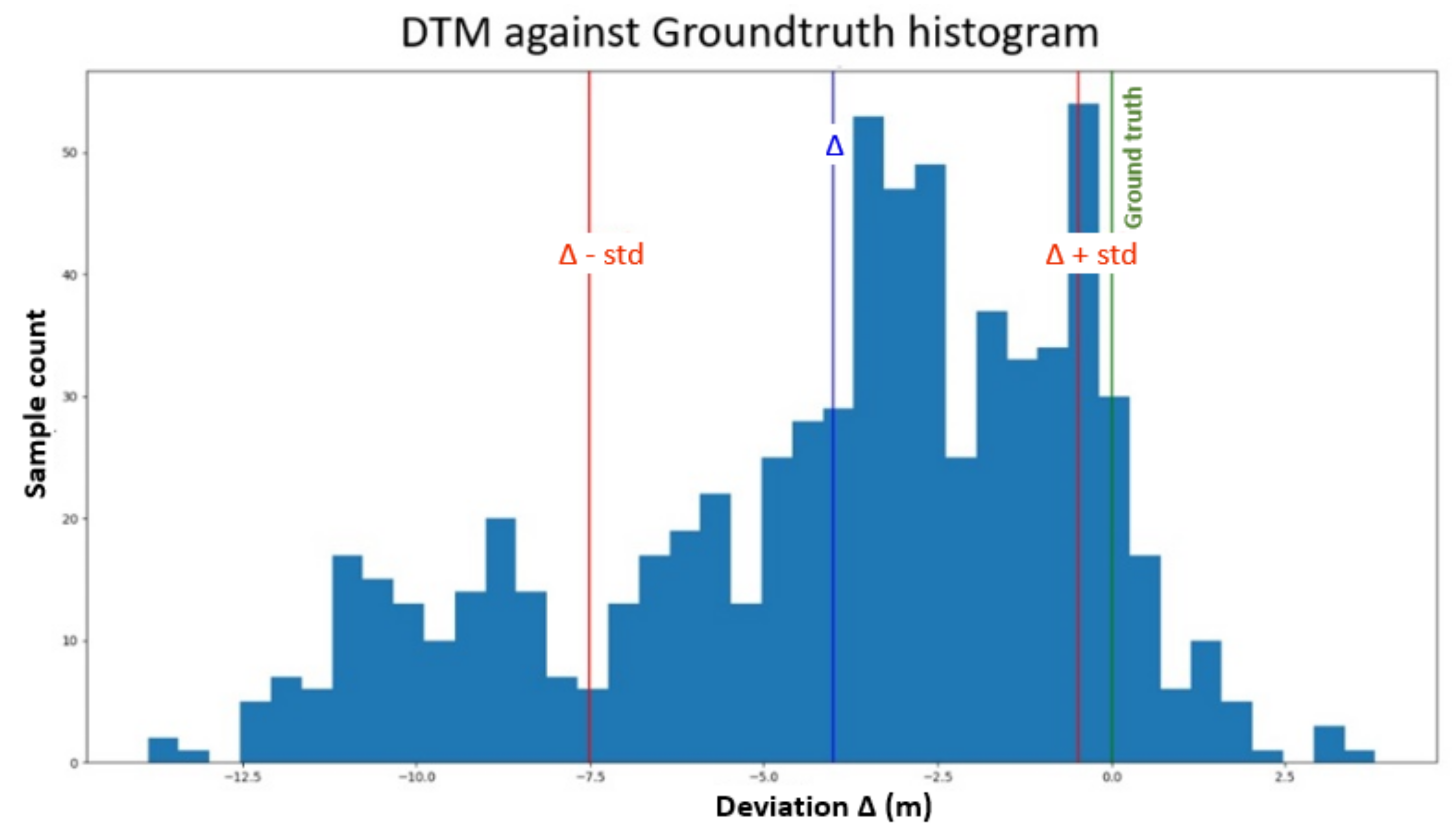
6.3. Uncertainties of Results

Unlike previous SDB methods, WCPE does not yield a unique—and possibly questionable—result, but a number of solutions, each associated with probabilities of occurrence.

The IHO traditional 95% precision requirement applicable to direct measurements of depths is irrelevant and must be replaced by other criteria such as a measure of dispersion to qualify the confidence of SDB depth assessments. For instance, a simple single decision could be computed by ponderating depth values by the density observed along the water column, as displayed in Figure 6, but the unique depth value thus determined would have to be further qualified by calculating standard deviations ponderated in a similar manner, in which case traditional error bars could be replaced by the module of standard deviation. New standards will have to be agreed upon by the IHO and the official Hydrographic Offices. Looking at the past, this might take a long time.

Five years ago, ARGANS tried with limited success to introduce SDB in the IHO Project Team tasked with updating the IHO S-44 standards for Hydrographic Surveys (HSPT). Eventually, a subgroup named “Satellite-Derived Bathymetry Best Practice Project Team” (SDB-PT) was set up, but the difference in comprehension between confirmed SDB developers and today’s Hydrographic Offices is important and several years of practice and further progresses will be needed to bridge the gap between academic theorists and hydrographic practitioners to get the most of satellite-derived bathymetry.

7. Conclusions

Unlike other SDB methods that do not provide the tools to filter rigorously and eliminate improbable depth values, WCPE has the potential to become the magic wand Seabed 2030 needs to fill the coastal gaps. It can propagate its parameters to all the world’s unknown areas provided the seafloor is visible from space and a reasonable amount of automation is implemented to facilitate this enormous task.

Bar seawater opacity, nothing now could prevent the coastal areas worldwide from being entirely covered down to the local cut-off values of light penetration in the ocean for an affordable cost.

The following significant results were achieved or confirmed:

• The proven ability of Sentinel-2 models, above the light penetration threshold, to provide depths to an order of accuracy of about one metre, without bias. The consequence of this potential revolution is being recognised with difficulty by professional users who tend to abandon the task of developing their own expertise and rely more and more on blind commercial contracts with service providers.
• The confirmation that high-resolution public time series such as Sentinel-2 achieve far better results than individual commercial VHR images plagued by biases and noise when used on their own, not to mention cost considerations.
• However, VHR model biases can be improved by association with lesser resolution models inferred from time series.
• The disappointing capacity of satellite images at this stage of development, whatever the resolution, to detect small structures with sufficient guarantee to abide by IHO safety of navigation standards embodied in the S-44 publication.
• WCPE parameters and inferred models can be propagated theoretically from a proven area to the next without requiring further ground controls. This outstanding asset must be tested further and the algorithms developed accordingly.
• Thanks to free public imagery, SDB has the proven capacity to meet the Seabed 2030 requirements for very affordable costs.

Whilst the IHO appropriate structures progress in their understanding of SDB and develop the standards this methodology requires to be fully accepted by the mariners and the international hydrographic community, the theoretical limits of SDB can continue to be improved with further trials and better monitoring of the factors that affect the water column, starting with the effects of turbidity which remain broadly unquantified.

References

1. Le Gouic, M. Etude des Applications Bathymétriques d’un Radiomètre Canal Bleu Embarqué sur Satellite, à Partir des Données d’une Simulation Aéroportée; Rapport D’étude n° 0002/85 EPSHOM: 21 p.; SHOM: Brest, France, 1983. [Google Scholar]
2. Laporte, J.; Dolou, H.; Avis, J.; Arino, O. Thirty years of Satellite Derived Bathymetry: The charting tool that Hydrographers can no longer ignore. Int. Hydrogr. Rev. 2020, 25, 129–154. [Google Scholar]
3. Polcyn, F.C.; Brown, W.L.; Sattinger, I.J. The Measurement of Water Depth by Remote Sensing Techniques; Michigan University Ann Arbor Institute of Science and Technology: Ann Arbor, MI, USA, 1970. [Google Scholar]
4. Lyzenga, D.R. Analysis of cladophora distribution in lake Ontario using remote sensing. Remote Sens. Environ. 1975, 4, 37–48. [Google Scholar]
5. Lee, Z.; Carder, K.L.; Mobley, C.D.; Steward, R.G.; Patch, J. Hyperspectral remote sensing for shallow waters. I. A semianalytical model. Appl. Opt. 1998, 37, 6329–6338. [Google Scholar] [PubMed]
6. Hedley, J.; Roelfsema, C.; Phinn, S.R. Efficient radiative transfer model inversion for remote sensing applications. Remote Sens. Environ. 2009, 113, 2527–2532. [Google Scholar] [CrossRef]
7. Malinas, N.P.; Lyzenga, D.R.; Tanis, F.J. Multispectral bathymetry using a simple physically based algorithm. IEEE Trans. Geosci. Remote Sens. 2006, 44, 2251–2259. [Google Scholar]
8. Byrd, R.H.; Lu, P.; Nocedal, J.; Zhu, C. A limited memory algorithm for bound constrained optimization. SIAM J. Sci. Stat. Comput. 1995, 16, 1190–1208. [Google Scholar] [CrossRef]
9. Zhu, C.; Byrd, R.H.; Nocedal, J. L-bfgs-b: Algorithm 778: L-bfgs-b, fortran routines for large scale bound constrained optimizationn. ACM Trans. Math. Softw. 1997, 23, 550–560. [Google Scholar] [CrossRef]
10. Morales, J.L.; Nocedal, J. L-bfgs-b: Remark on algorithm 778: L-bfgs-b, fortran routines for large scale bound constrained optimization. ACM Trans. Math. Softw. 2011, 38, 1–4. [Google Scholar] [CrossRef]
11. Celik, S.; Korkmaz, M. Beta distribution and inferences about the beta functions. Asian J. Sci. Technol. 2016, 7, 2960–2970. [Google Scholar]
12. Schreiber, J. Pomegranate: Fast and flexible probabilistic modelling in python. J. Mach. Learn. Res. 2018, 18, 1–6. [Google Scholar]
13. Cui, S.; Datcu, M. Comparison of Kullback-Leibler divergence approximation methods between gaussian mixture models for satellite image retrieval. In Proceedings of the 2015 IEEE International Geoscience and Remote Sensing Symposium (IGARSS), Milan, Italy, 26–31 July 2015; pp. 3719–3722. [Google Scholar]
Figure 1. An ageless reference: the first satellite-based nautical chart ever produced by a Governmental Hydrographic Office: Atolls of Ouvéa and Beautemps-Beaupré (1990).
Remotesensing 14 04484 g001
Figure 2. ARGANS 2015 optimistic projection of SDB products compliance with S-44 orders of precision.
Remotesensing 14 04484 g002
Figure 3. A rather uninspiring, although not uncharacteristic, histogram of a 500 sq.km AOI. The ≈ 4 m bias and 3.5 m Std are not compatible with a 2-m grid resolution (Sentinel-2 image—Traditional Lee et al. SDB model—NE Qatar).
Remotesensing 14 04484 g003
Figure 4. Lyzenga and Lee et al. fundamental problem: one pixel, several possible interpretations.
Remotesensing 14 04484 g004
Figure 5. Comparison of Guadeloupe scatterplot and histogram against S-44 orders of precision. IHO S-44 Compliancy cannot be met in large zones.
Remotesensing 14 04484 g005
Figure 6. A depths density profile against 490 nm spectral reflectance. Sentinel-2 time series—Guadeloupe.
Remotesensing 14 04484 g006
Figure 7. Traditional Lee et al. RTE.
Remotesensing 14 04484 g007
Figure 8. Extraction of probable depth within an ROI polyexp-beta-normal distribution.
Remotesensing 14 04484 g008
Figure 9. Four test zones and four satellite constellations to prove the new concept. (a) West Indies first exploration, (b) Madagascar, (c) French Polynesia, (d) Qatar.
Remotesensing 14 04484 g009aRemotesensing 14 04484 g009b
Figure 10. Influence of parameters a, b, and c from Lyzenga’s equation. (a) Simple instance of BNP. (b) Same BNP with higher attenuation coefficient c. (c) Same BNP but with different parameters a and b.
Remotesensing 14 04484 g010
Figure 11. Influence of the σ dispersion parameter. (a) low σ. (b) average σ. (c) High σ.
Remotesensing 14 04484 g011
Figure 12. Influence of α and β parameters. (a) α < β. (b) α = β. (c) α > β.
Remotesensing 14 04484 g012
Figure 13. Ground truth provided by a single sounding line in Tahanea. (a) World View image and supporting ENC cross-section in red. (b) Scatter plot of blue Depth/Reflectance data.
Remotesensing 14 04484 g013
Figure 14. Example of two distinct depth-constrained water-column profiles. Each cloud of points (red and blue) were generated from a BNP with different parameters.
Remotesensing 14 04484 g014
Figure 15. Regressing BNP parameters from the ground truth data displayed in Figure 13. (a) Regression of a cloud of points (blue crosses) to determine parameters a, b and c. (b) Using inferred parameters a, b and c to deduce statistical parameters σ, α and β.
Remotesensing 14 04484 g015
Figure 17. Example of a BNP mixture with four components.
Remotesensing 14 04484 g017
Figure 18. Ground truth provided by multiple sounding lines in Tahanea. (a) World View image and supporting ENC cross-sections in red, (b) Scatter plot of blue Depth/Reflectance data.
Remotesensing 14 04484 g018
Figure 19. Regression using a mixture of two BNPs.
Remotesensing 14 04484 g019
Figure 20. Splitting a BNP distribution along its depth axis. (a) Sample points inadequately covered by a single BNP distribution. (b) Splitting the samples with a 2-component β-distribution mixture. (c) The two resulting BNP distributions.
Remotesensing 14 04484 g020
Figure 21. Splitting a distribution along the reflectance axis (relative to curve offset). (a) Sample points inadequately covered by a single BNP distribution. (b) Splitting the samples with a 2-component Gaussian mixture. (c) The two resulting BNP distributions.
Remotesensing 14 04484 g021
Figure 22. Inference of the attenuation coefficient c in a two-component BNP mixture for a given input reflectance (horizontal green line). The sample cloud is made of red and blue points, each artificially generated from two BNPs respectively.
Remotesensing 14 04484 g022
Figure 23. Example of a cloud of depth-green-blue samples and a trained multispectral BNP mixture. The cloud of samples (in faded blue) consist of two distinguishable sub-cloud. Green points are the projection of those samples unto depth-blue plane, Blue points are the projection unto depth-green plane. Those projection planes are analogous to scatter plots exhibited in previous sections.
Remotesensing 14 04484 g023
Figure 24. Example of a cloud of deep green-blue samples mixed with a trained multispectral BNP.
Remotesensing 14 04484 g024
Figure 25. The 3rd Madagascar area of interest. (a) Original chart (1915) based on the reconnoitre survey; (b) the 3rd AOI’s suspended particular matter.
Remotesensing 14 04484 g025
Figure 26. (a) Pleiades’ reflectances/depths plot; (b) WCPE density plot after training. Note the very homogeneous, almost linear environment.
Remotesensing 14 04484 g026
Figure 27. WCPE/Groundtruth scatter plot and Pleiades/WCPE histogram. (a) WCPE/Groundtruth scatter plot; (b) Pleiades/WCPE histogram.
Remotesensing 14 04484 g027
Figure 28. WorldView statistical analysis. (a) WV/Groundtruth scatter plot; (b) WorldView histogram; (c) WV density plot.
Remotesensing 14 04484 g028
Figure 29. Persian Gulf min and max downward visibility (source: SHOM’s Mars model).
Remotesensing 14 04484 g029
Figure 30. Qatar’s two test areas of interest.
Remotesensing 14 04484 g030
Figure 31. Comparison between WCPE/IDA harmonised DTM and ground truth. The depth of penetration is limited to 11/15 m due to turbidity.
Remotesensing 14 04484 g031
Figure 32. Typical cross sections comparing methods and satellite images of different resolutions. (a) VHR best single image vs Sentinel-2 time series modellised with WCPE, (b) The same, modellised with traditional SDB. Note the VHR poor signal/noise ratio.
Remotesensing 14 04484 g032