Assessment of Material Layers in Building Walls Using GeoRadar

Abstract

Assessing the structure of a building with non-invasive methods is an important problem. One of the possible approaches is to use GeoRadar to examine wall structures by analyzing the data obtained from the scans. However, so far, the obtained data have to be assessed manually, relying on the experience of the user in interpreting GPR radargrams. We propose a data-driven approach to evaluate the material composition of a wall from its GPR radargrams. In order to generate training data, we use gprMax to model the scanning process. Using simulation data, we use a convolutional neural network to predict the thicknesses and dielectric properties of walls per layer. We evaluate the generalization abilities of the trained model on the data collected from real buildings.

1. Introduction

Assessing the recycling costs of existing buildings often requires a destructive method to look through its building elements such as walls and floors. In order to answer what materials comprise a wall, one has to obtain an explicit overview of the cross-section—either by drilling or carving out a piece. Ground-penetrating radar (GPR) offers a way to examine the walls without a destructive invasive process. GeoRadar has been successfully utilized for non-destructive examination in other fields, such as archaeology [1], seismology [2], or civil engineering [3,4].

In order to identify materials in layered structures, one could refer to research for a similar problem, namely, obtaining permittivity maps from GPR radargrams [5]. Previous research concentrated on using machine learning to invert radargrams into permittivity maps, i.e., to receive per-pixel permittivity values as a reconstruction of the original scene. Ref. [6] used Deep Neural Networks to reconstruct tunnel linings, while [5] showed an improvement of the idea and its application to more general sub-surface structures.

Ref. [7] used deep learning to estimate the size parameters of reinforcement bars by combining GPR and electromagnetic induction. Ref. [8] used convolutional neural networks (CNN) to invert electrical resistivity data. Ref. [2] used CNNs for the interpretation of seismic images. Aside from deep learning methods, there are other representatives of the family of data-driven approaches. A method called Full Wave Inversion (FWI) aims at minimizing the differences between recorded and modeled waveforms and adjusts the model to fit the observations [9]. Another method, the linear inverse scattering algorithm [10], tries to reconstruct target objects from the scattered electric field and has been used for archaeological surveys [11].

In order to reduce the number of parameters to be learned (a full grid representation of the permittivity map), we propose to simplify the representation to a sequence of layers. We predict the width and the permittivity of the underlying material for each layer by using a convolutional neural network (CNN). The proposed CNN was trained and evaluated on a dataset of simulated B-scans. Moreover, we collected radargrams of real buildings and validated the proposed CNN on this dataset.

2. Methodology

The output of the GPR scanning process is a radargram. It is a 2D array (also called B-scan, see Figure 1) of electric field strength values, where each column (also called A-scan) corresponds to the field strength over time for one spatial position along the scanning direction. Analyzing such radargrams manually is a laborious process. Objects of different permittivities and sizes will affect the traveling velocity of the source wave. Such behavior can be seen in Figure 2, Figure 3 and Figure 4, which show the results of scanning simulations in a setup with a solid material block for one column (spatial location) of the radargram. Therefore, the goal is to determine the traveling velocities of the waves, allowing to estimate the dielectric properties of the material in the examined object. The Figure 2 and Figure 3 demonstrate the effect of a permittivity change and a thickness change, which can be observed to strongly influence the wave’s velocities. The change in conductivity mostly affects the amplitudes and not the velocities, as can be seen in Figure 4.

In this work, we employ a Convolutional Neural Network (CNN) as a model for predicting material layers of walls from B-scans. In particular, the CNN predicts the thicknesses and relative permittivities of each layer. CNNs have been performing very successfully in tasks of computer vision and image classification [12,13]. Neural networks approximate a function by constructing a sequence of parameterized computations. Its parameters or weights are adjusted through an iterative process that minimizes the goal function that encodes an objective.

2.1. CNN Architecture

We employ a convolutional neural network (CNN) that takes input B-scans. Here, B-scans are represented by two-dimensional arrays of a size of 255x40. They are then passed to a sequence of convolutional maps of a kernel size of 20x5. We employ six blocks of convolutional layers that are activated with the ReLU function. ReLU (Rectified Linear Unit) has been recognized as one of the best choices for the activation function [14]. It is defined as the positive truncate of the incoming argument: $\mathbf{ReLU}\left(\mathbf{x}\right)=\mathbf{max}(\mathbf{0},\mathbf{x})$. The result is then batch normalized in order to stabilize the network’s training by re-centering and re-scaling the output of the previous layer. The number of the output feature maps in each such block differs slightly. We use the following sizes: 8, 16, 32, 16, 8, 4, similar to the depiction in Figure 5.

The output of the last convolutional layer is then flattened and processed by five fully connected linear layers activated with hyperbolic tangents. The hyperbolic tangent is another common activation function, which displayed a better performance in our experiments. The sizes of the linear layers were set as 5000, 2000, 800, 300, and 12. The final layer has two groups of neurons. The first 6 neurons in the final layer encode thicknesses of the material layers, whereas the next 6 neurons are responsible for the permittivities. In order to ensure positive output values, we employ a softplus function, which is a smooth approximation of the ReLU function. The difference between the outputs of the model and corresponding targets from the datasets are computed with the L1 loss, which computes an absolute norm of the difference. This is then used to compute the gradients and optimize network parameters.

3. Datasets

3.1. Simulated 2D Dataset

In order to test the hypothesis that our network architecture can predict material layers, we created a clean dataset containing $30,000$ simulated GPR B-Scans, thus, avoiding problems due to real-world imperfections. For the simulation, we used the GprMax software [15], which is based on a finite-difference time-domain simulation method. We set up a 2D grid that was 24 cm wide and 46 cm thick. It was filled with solid material blocks whose total thickness was up to 46 cm. The set of used relative permittivities was 1 to 7, which represents a typical range for construction materials. Another dielectric parameter, conductivity, was not considered in this work, since it mostly affects amplitudes, as is visible in Figure 4, whereas the important characteristics of a material are determined by the traveling time of the transmitted wave through that medium.

The transmitter and receiver antennae were set 40 mm apart, with the transmitting frequency being 1 GHz and the source waveform being the Ricker wavelet [16]. The transmitting time window was 12 nanoseconds at a fixed position. After the simulation was complete, we extracted the electrical component in the transverse direction of the simulated electromagnetic field and saved it as a B-scan. Together with the information about the material class and thickness of the material block, it formed a sample of the dataset.

The corresponding targets in the dataset—the wall configurations—were represented by a stack of up to 6 rectangular blocks. The combinations of different material layers were generated randomly. First, we uniformly sampled the number of layers. Next, we sampled the thicknesses and permittivities from a multinomial distribution, which is a generalization of a binomial distribution. It allowed us to sample several variables (thicknesses) at once and avoid the issue when most of the given volume was taken by the first layers. Since there were up to 6 layers, there were 12 variables encoding a target in a configuration: 6 for thickness and 6 for relative permittivity. Furthermore, since the prediction of the further layers is more difficult, we filled the dataset with more instances of the more layered structures, as can be seen from the distribution of the samples over the number of layers in Figure 6.

In order to consider conditions closer to an actual environment, we added noise grains that varied in size and permittivity. The two small dots at the top are transmitter and receiver antennas. The blocks of shades of blue are material layers, whereas the small colored objects are the noise grains.

Examples of three simulation scenes are shown in Figure 1. They illustrate three-layered structures of different thicknesses and materials. The detailed descriptions of the scenes’ parameters are given in

Table 1. Parameters of the scenes’ setups in Figure 1.

Thicknesses	Layer 1	Layer 2	Layer 3
Scene 1	0.128	0.105	0.143
Scene 2	0.063	0.065	0.042
Scene 3	0.05	0.05	0.05
Permittivities	Layer 1	Layer 2	Layer 3
Scene 1	4.283	4.3725	5.516
Scene 2	5.423	5.226	2.991
Scene 3	6.278	7.584	5.841

. From the tables and Figure 1, one can see that the relation between the position of the amplitude peaks (a ripple on a radargram) and the actual medium change is not linear. For example, scenes 2 and 3 have very similar layer thicknesses, but due to differences in permittivities, the ripples appear at very different times on B-scans 2 and 3: two ripples at around 3ns in B-scan 2, one ripple at 3.2ns and another one at 6.2ns in B-scan 3.

3.2. Real Dataset

In order to validate our approach on real data, we also collected a set of radargrams from nine buildings. Each building had walls that could be clustered into groups of a certain build. The builds constituted a composition of layers of certain thicknesses and materials. Some builds had materials that were non-homogeneous in their structure, e.g., reinforced concrete or patterned woodwork. Capturing such structures is not within the scope of this project, hence, those builds were discarded.

The scans were taken with the pulseEKKO radar equipment, which has a central frequency of 1 GHz. Possible sources of electromagnetic radiation that could disturb the scanning process were avoided. The obtained scans underwent various pre-processing steps. First, the direct current signal component was removed in order to compensate for the constant bias shift, and the recorded traces were re-centered around zero. Then, we filtered out the frequencies below 500 MHz to compensate for noise. Even though we tried to avoid potential electromagnetic distortion sources, it was not possible to avoid the EM background completely. Finally, a time-zero correction was performed: the starting times of the first waves for each scan were established, and the traces were shifted so that they started with time-zero.

The building walls had various widths, which subsequently resulted in the non-uniform width of B-scans in the dataset. Therefore, we cut the scans into segments of a fixed length of 40 traces in the width dimension. The cuts were carried out at random locations within the B-scan, because the scans of the real buildings can contain various artifacts such as cables, voids and pipes. By providing several cuts per scan, we allowed the CNN to learn on several samples that represent the same material configuration, thus, making it more robust to noise. Altogether, the dataset comprised 3400 samples.

The covered materials are listed in Appendix A. Some materials that were similar in structure and their dielectric properties were grouped together. The relative permittivities were collected from various sources [17,18,19].

4. Results

4.1. Evaluation on Simulated Data

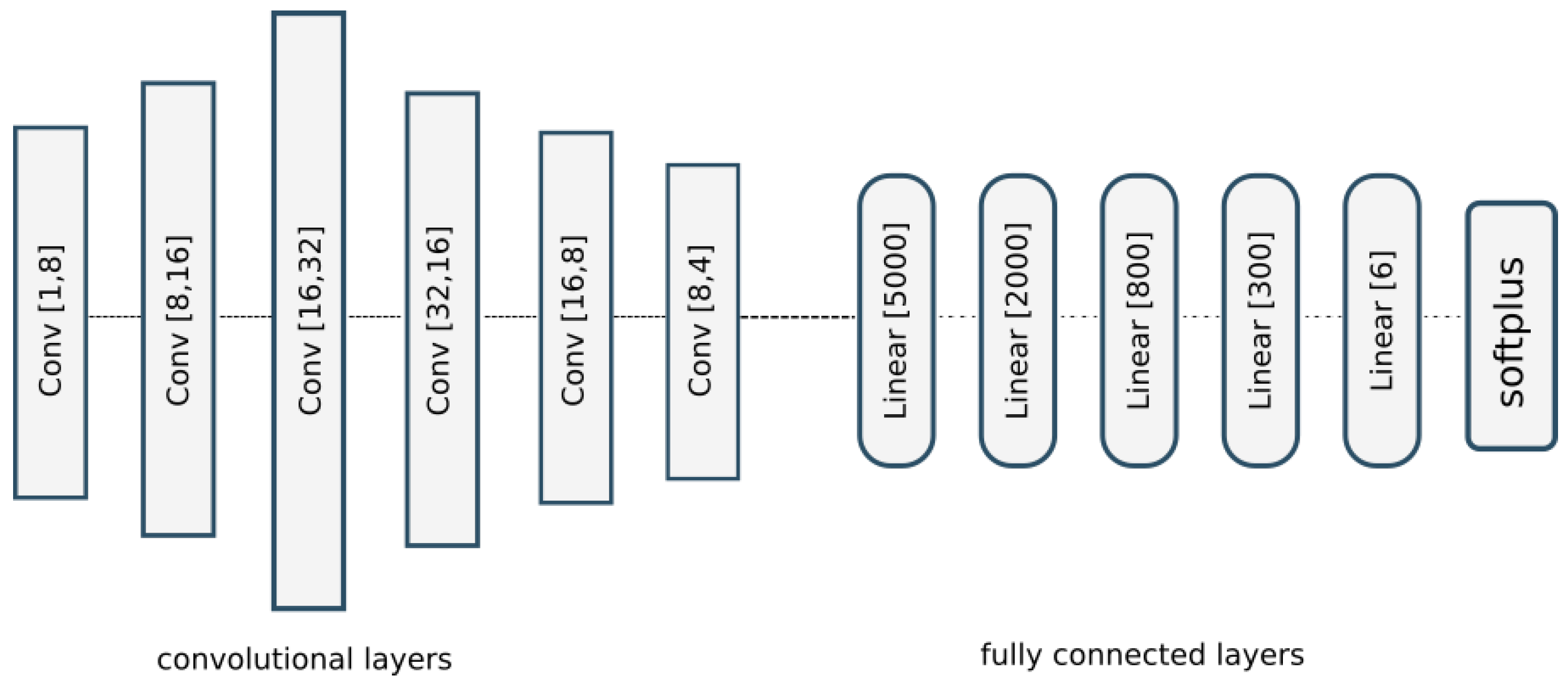
The previously described simulated data were used to train the convolutional neural network from Section 2.1. We split the dataset into training and testing sets in a ratio of 80 to 20. The CNN was trained for 1500 epochs. The network parameters were optimized with the ADAM optimizer with a step length of 0.001.

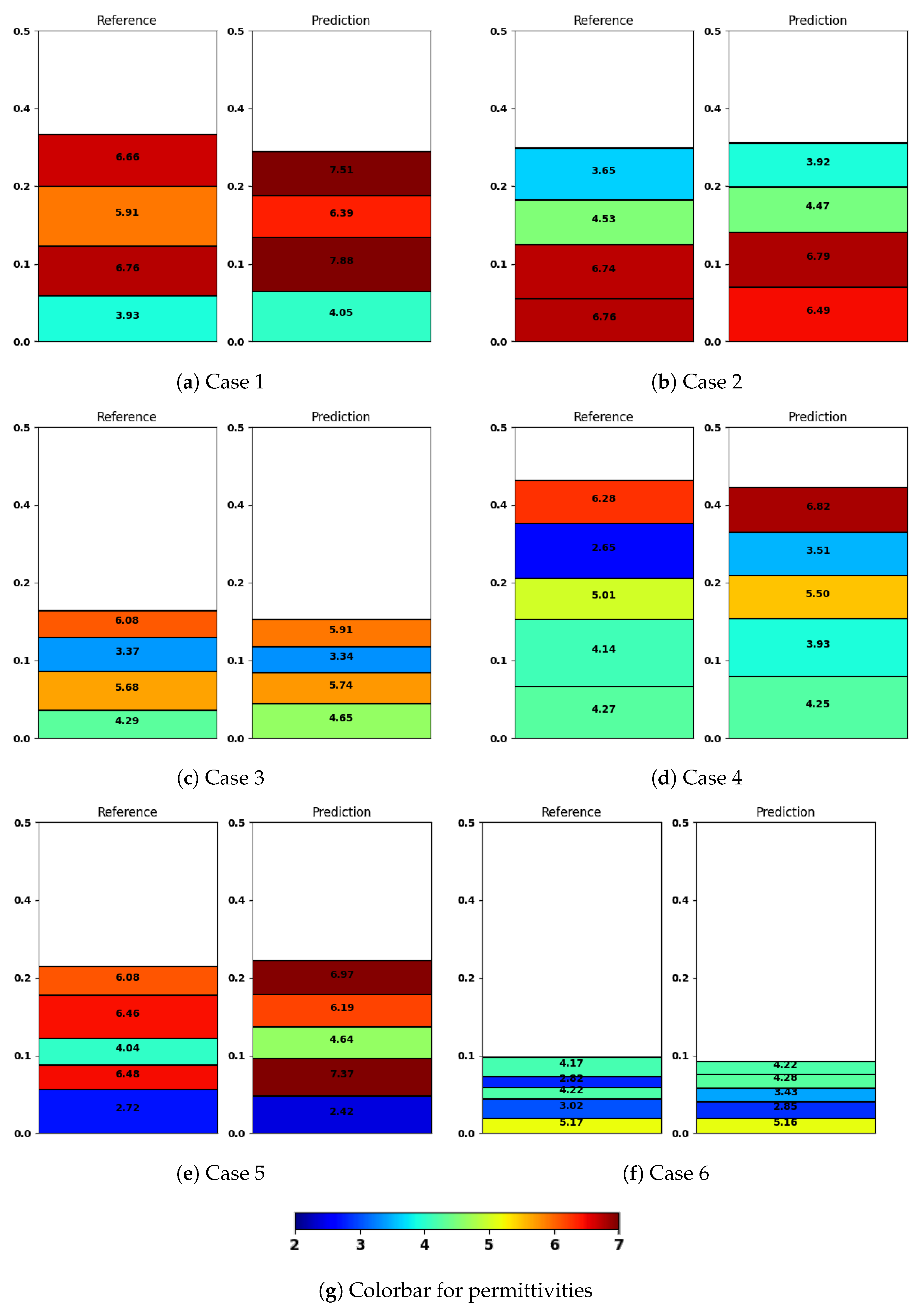
The results of the CNN’s performance are visualized in Figure 7, where we show six examples from the test dataset (left) together with the output of our trained model (right). We omitted the structures with few layers in this visualization in order to showcase the more complex cases, but we provide such results in

Table 2. Statistics on the simulated dataset considering only three layers.

Total Mean Thickness Error	Average Value	Average Value in Percentage
Training	8 mm	9.5%
Test	13 mm	4.0%
Total Mean Permittivity Error	Average Value	Average Value in Percentage
Training	0.19	15.8%
Test	0.69	14.7%

. We observe that low permittivity layers negatively affect the quality of prediction in further layers, as can be seen in Figure 7a,b,e. In Case 1 from Figure 7a, the first layer has a permittivity of 3.93, which is predicted fairly close by the model to be 4.05. However, the prediction error in subsequent layers is already more significant, ranging from 0.48 to 1.12. A similar situation appears in Case 5 from Figure 7e. The first layer has a permittivity of 2.72, and its thickness and permittivity are predicted quite well by the model, but the further layers have a visible divergence from the reference configuration both in terms of thicknesses and permittivities. The opposite situation can be observed in Case 2 from Figure 7b. The first layer has a quite high permittivity—6.76. The range of prediction errors for the further layers stays between 0.05 and 0.27, and even around 0.05–0.06 for the first layers, which is a significantly better prediction than with the previously mentioned cases. A similar behavior can be observed in cases Figure 7c,d. In Case 6 from Figure 7f, we can also see an accurate prediction of the first layers with high permittivity. However, due to the second layer having a low permittivity value of 3.02, the prediction errors in the further layers rapidly increase, going from 0.79 to 1.46.

Statistics over the whole dataset are shown in

Table 3. Statistics on the simulated dataset.

Total Mean Thickness Error	Average Value	Average Value in Percentage
training	9.3 mm	10.1%
test	10.2 mm	3.3%
Total Mean Permittivity Error	Average Value	Average Value in Percentage
training	0.71	16.4%
test	0.81	14.9%

, where the average error values in thickness and permittivity are presented. The errors in thickness amounted to 9.3 mm in thickness for the training set and 10.2 mm for the test set. The values are also presented as percentages and compared against average thicknesses and permittivities of the whole dataset—10.1% for the training set and 3.3% for the test set. Given that the estimated vertical resolution for the antenna of central frequency 1 GHz is about 2.5 cm [20], the achieved results are adequate. Regarding the permittivities, the average training and test errors are 0.71 and 0.81, respectively. As mentioned in the previous section, we used the permittivity range between 1 and 7. This means that achieving average permittivity errors below 1 demonstrates a good model performance.

We also considered a dataset with fewer layers. The statistics are presented in Table 2. The values show very similar performances. Moreover, on this dataset, we were able to better predict permittivities on average compared to the six-layer cases. However, the results show a slightly higher error value for thickness predictions on the test set.

Additionally, we provide per-layer error values in

Table 4. Thickness and permittivity errors on the simulated dataset for each layer.

	Layer 1	Layer 2	Layer 3	Layer 4	Layer 5	Layer 6
Mean thickness error (training)	15.2%	17.9%	19.2%	21%	23.3%	25.8%
Mean thickness error (test)	16.9%	19.9%	21.5%	23.4%	26%	28.8%
Mean permittivity error (training)	14.8%	14.7%	14.6%	14.6%	14.6%	14.7%
Mean permittivity error (test)	17.2%	17.1%	17.0%	16.9%	17.0%	17.1%

. It can be observed that the prediction of thicknesses worsens at deeper layers, which is to be expected, considering the dissipation of signals going through the previous layers. The effect is, however, not present for permittivities. Their prediction remains stable throughout the layers within the one percent range.

Overall, we can conclude that the proposed network architecture achieves good results on the simulated data.

4.2. Evaluation on Actual Buildings

We evaluated the network architecture on the described real dataset. We tested two modes: one using only the real data as input, and one using transfer learning, where we pre-trained the model on the simulated dataset and then let it train on the collected dataset. The idea of using transfer learning is that the network could generalize beyond the input seen in the real-world training data. This is important because the training data contain only a limited number of typical wall builds.

Both modes were trained for 500 epochs. The results are shown in

Table 5. Results of transfer learning. The model trained on the collected dataset only shows a better performance than the model pre-trained on the simulated dataset.

Total Mean Thickness Error	Model Pre-Trained on Simulated Data	Model Trained on Real-Data Only
Training	13.6 mm (11.6%)	12.9 mm (10.1%)
Test	17.8 mm (7.7%)	15.3 mm (2.0%)
Total Mean Permittivity	Model Pre-Trained on Simulated Data	Model Trained on Real-Data Only
Training	0.36 (18.2%)	0.17 (14.8%)
Test	0.5 (11.8%)	0.29 (5.7%)

and

Table 6. Per-layer comparison of the pre-trained model and the untrained (collected data only) model in terms of thickness and permittivity. Lower errors at layer 2 could be related to the fact that the materials at this layer varied less than on the other levels.

Model Pre-Trained on Simulated Data	Layer 1	Layer 2	Layer 3	Layer 4	Layer 5	Layer 6
Mean thickness error (training)	24.4%	5.4%	18.5%	55.1%	137.6%	-
Mean thickness error (test)	38.2%	8.5%	29.0%	86.3%	215.4%	-
Mean permittivity error (training)	6.9%	10.1%	9.1%	5.1%	6.1%	-
Mean permittivity error (test)	10.5%	15.3%	13.8%	7.8%	9.3%	-
Model Trained on Real-Data Only	Layer 1	Layer 2	Layer 3	Layer 4	Layer 5	Layer 6
Mean thickness error (training)	21.2%	4.7%	16.1%	48.0%	119.7%	-
Mean thickness error (test)	31.0%	6.9%	23.5%	69.9%	174.6%	-
Mean permittivity error (training)	1.8%	2.7%	2.4%	1.4%	1.6%	-
Mean permittivity error (test)	5.1%	7.5%	6.7%	3.8%	4.5%	-

.

It can be seen that the pre-trained model does not demonstrate better performance. Results on the training part of the collected dataset are slightly better for the untrained model and significantly better on the test dataset for the untrained model, too. The reason for this performance difference lies in the deviation between the simulated and the collected data; the simulated data cover a larger variation of wall builds, and can, therefore, be expected to generalize better to unseen builds, however, at the cost of a lower performance for the wall builds that are actually contained in the data. Evaluating this generalization in more depth is the subject of future work.

Furthermore, the task of generating realistic data that are similar to the output of the target device is difficult due to the problem of reproducing the device model. We used the same antenna frequency in the simulation as the device we utilized, but other factors are as important, including antenna geometry, radiation pattern, etc. These factors made the simulated B-scans considerably different from the ones we collected.

The network that was trained only on the real data demonstrates high performance in terms of material classification accuracy and precision of thickness prediction. As

Table 7. Comparison with the pre-trained model in terms of accuracy of the material classification. Better accuracy is demonstrated by the model trained only on the collected data.

	Model Pre-Trained on Simulated Data	Model Trained on Real-Data Only
Accuracy (training)	90%	92%
Accuracy (test)	82%	90%

shows, it achieves an accuracy of 92% on the training set and 90% on the test set. The classification was implemented by assigning a material with the closest permittivity value, and thus, depends on the prediction of permittivities. The precision of permittivity prediction is shown in Table 5. It shows an average error of 0.17 for the training set and 0.29 for the test set, which is a favorable result since the construction materials’ permittivity range is typically 1 to 7. In terms of predicting layer thicknesses, we can see the errors of 12.9 mm and 15.3 mm for training and test sets. These values are higher than the ones obtained from training the CNN on the simulated dataset. However, the demonstrated performance is as expected, considering that the dataset with real scans contains noisier, more complex data and the fact that wall thicknesses can reach 40 cm.

5. Conclusions

In this paper, we investigated the application of deep learning for the non-invasive examination of wall material compositions using GeoRadar. We used a neural network consisting of convolutional as well as fully connected layers.

We first evaluated the network on a dataset consisting of simulated B-scans. The predictions on the validating dataset have shown adequate results, being able to closely identify materials in many-layered structures.

We then trained and tested the proposed network on the data collected from real buildings, both directly and using transfer learning, starting from the network pre-trained on the simulated data. The experiments showed little difference between the model pre-trained on the simulated data and the model trained on the real dataset only, with the second one demonstrating a slightly better performance. We observed a high accuracy of the material classification and a good precision of the layer thickness prediction for both of them.

The conducted research demonstrates promising results for future applications in the construction industry. Combining GeoRadar surveying with machine learning techniques could allow for a non-invasive investigation of wall structures and could drastically reduce examination costs.

In future work, we will evaluate the generalization capability of the pre-trained network by collecting more real datasets. We also plan to test recursive neural network architectures, which could potentially mitigate the problem of a prediction-quality drop at deeper material layers. We will also investigate the possibility of making the neural network less dependent on the specific GeoRadar antenna models.

References

- Zhao, W.; Forte, E.; Pipan, M.; Tian, G. Ground Penetrating Radar (GPR) attribute analysis for archaeological prospection. J. Appl. Geophys. 2013, 97, 107–117. [Google Scholar] [CrossRef]
- Zheng, Y.; Zhang, Q.; Yusifov, A.; Shi, Y. Applications of supervised deep learning for seismic interpretation and inversion. Lead. Edge 2019, 38, 526–533. [Google Scholar] [CrossRef]
- Morris, I.; Abdel-Jaber, H.; Glisic, B. Quantitative Attribute Analyses with Ground Penetrating Radar for Infrastructure Assessments and Structural Health Monitoring. Sensors 2019, 19, 1637. [Google Scholar] [CrossRef] [PubMed]
- Alperovich, L.; Eppelbaum, L.; Zheludev, V.; Dumoulin, J.; Soldovieri, F.; Proto, M.; Bavusi, M.; Loperte, A. A new combined wavelet methodology: Implementation to GPR and ERT data obtained in the Montagnole experiment. J. Geophys. Eng. 2013, 10, 025017. [Google Scholar] [CrossRef]
- Ji, Y.; Zhang, F.; Wang, J.; Wang, Z.; Jiang, P.; Liu, H.; Sui, Q. Deep Neural Network-Based Permittivity Inversions for Ground Penetrating Radar Data. IEEE Sens. J. 2021, 21, 8172–8183. [Google Scholar] [CrossRef]
- Liu, B.; Ren, Y.; Liu, H.; Xu, H.; Wang, Z.; Cohn, A.G.; Jiang, P. GPRInvNet: Deep Learning-Based Ground-Penetrating Radar Data Inversion for Tunnel Linings. IEEE Trans. Geosci. Remote Sens. 2021, 59, 8305–8325. [Google Scholar] [CrossRef]
- Li, X.; Liu, H.; Zhou, F.; Chen, Z.; Giannakis, I.; Slob, E. Deep learning–based nondestructive evaluation of reinforcement bars using ground-penetrating radar and electromagnetic induction data. Comput.-Aided Civ. Infrastruct. Eng. 2021, Early View. Available online: https://onlinelibrary.wiley.com/doi/pdf/10.1111/mice.12798 (accessed on 7 August 2022). [CrossRef]
- Liu, B.; Guo, Q.; Li, S.; Liu, B.; Ren, Y.; Pang, Y.; Guo, X.; Liu, L.; Jiang, P. Deep Learning Inversion of Electrical Resistivity Data. IEEE Trans. Geosci. Remote Sens. 2020, 58, 5715–5728. [Google Scholar] [CrossRef]
- Kruk, J.; Liu, T.; Mozaffari, A.; Gueting, N.; Klotzsche, A.; Vereecken, H.; Warren, C.; Giannopoulos, A. GPR full-waveform inversion, recent developments, and future opportunities. In Proceedings of the 2018 17th International Conference on Ground Penetrating Radar (GPR), Rapperswil, Switzerland, 18–21 June 2018; pp. 1–6. [Google Scholar] [CrossRef]
- Gennarelli, G.; Soldovieri, F. A Linear Inverse Scattering Algorithm for Radar Imaging in Multipath Environments. IEEE Geosci. Remote Sens. Lett. 2013, 10, 1085–1089. [Google Scholar] [CrossRef]
- Persico, R.; Soldovieri, F.; Utsi, E. Microwave tomography for processing of GPR data at Ballachulish. J. Geophys. Eng. 2010, 7, 164–173. [Google Scholar] [CrossRef]
- Fang, W.; Love, P.E.; Luo, H.; Ding, L. Computer vision for behaviour-based safety in construction: A review and future directions. Adv. Eng. Inform. 2020, 43, 100980. [Google Scholar] [CrossRef]
- Sahiner, B.; Pezeshk, A.; Hadjiiski, L.M.; Wang, X.; Drukker, K.; Cha, K.H.; Summers, R.M.; Giger, M.L. Deep learning in medical imaging and radiation therapy. Med. Phys. 2019, 46, e1–e36. [Google Scholar] [CrossRef] [PubMed]
- Glorot, X.; Bordes, A.; Bengio, Y. Deep Sparse Rectifier Neural Networks. In Proceedings of the Fourteenth International Conference on Artificial Intelligence and Statistics, Fort Lauderdale, FL, USA, 11–13 April 2011; Gordon, G., Dunson, D., Dudík, M., Eds.; PMLR: Fort Lauderdale, FL, USA, 2011; Volume 15, pp. 315–323. [Google Scholar]
- Warren, C.; Giannopoulos, A.; Giannakis, I. gprMax: Open source software to simulate electromagnetic wave propagation for Ground Penetrating Radar. Comput. Phys. Commun. 2016, 209, 163–170. [Google Scholar] [CrossRef]
- Wang, Y. The Ricker wavelet and the Lambert W function. Geophys. J. Int. 2014, 200, 111–115. Available online: https://academic.oup.com/gji/article-pdf/200/1/111/33388581/ggu384.pdf (accessed on 21 June 2022). [CrossRef][Green Version]
- Effects of Building Materials and Structures on Radiowave Propagation above about 100 MHz. Recommendation ITU-R. 2015, p. 2040-1. Available online: https://www.itu.int/dms_pubrec/itu-r/rec/p/R-REC-P.2040-1-201507-S!!PDF-E.pdf (accessed on 2 February 2022).
- Ellingson, S.W. Electromagnetics; VT Publishing: Blacksburg, VA, USA, 2018; Volume 1. [Google Scholar] [CrossRef]
- Relative Permittivity—The Dielectric Constant. Engineering ToolBox. 2010. Available online: https://www.engineeringtoolbox.com/relative-permittivity-d_1660.html (accessed on 21 June 2022).
- Rial, F.; Pereira, M.; Lorenzo, H.; Arias, P.; Novo, A. Resolution of GPR bowtie antennas: An experimental approach. J. Appl. Geophys. 2009, 67, 367–373. [Google Scholar] [CrossRef]
Publisher’s Note: MDPI stays neutral with regard to jurisdictional claims in published maps and institutional affiliations. |
© 2022 by the authors. Licensee MDPI, Basel, Switzerland. This article is an open access article distributed under the terms and conditions of the Creative Commons Attribution (CC BY) license (https://creativecommons.org/licenses/by/4.0/).