3D LoD2 and LoD3 Modeling of Buildings with Ornamental Towers and Turrets Based on LiDAR Data

Abstract

This paper presents an innovative approach to the automatic modeling of buildings composed of rotational surfaces, based exclusively on airborne LiDAR point clouds. The proposed approach starts by detecting the gravity center of the building’s footprint. A thin point slice parallel to one coordinate axis around the gravity center was considered, and a vertical cross-section was rotated around a vertical axis passing through the gravity center, to generate the 3D building model. The constructed model was visualized with a matrix composed of three matrices, where the same dimensions represented the X, Y, and Z Euclidean coordinates. Five tower point clouds were used to evaluate the performance of the proposed algorithm. Then, to estimate the accuracy, the point cloud was superimposed onto the constructed model, and the deviation of points describing the building model was calculated, in addition to the standard deviation. The obtained standard deviation values, which express the accuracy, were determined in the range of 0.21 m to 1.41 m. These values indicate that the accuracy of the suggested method is consistent with approaches suggested previously in the literature. In the future, the obtained model could be enhanced with the use of points that have considerable deviations. The applied matrix not only facilitates the modeling of buildings with various levels of architectural complexity, but it also allows for local enhancement of the constructed models.

1. Introduction

Remote measurement systems enable the development of digital models that depict real-world objects with increasing accuracy. Light detection and ranging (LiDAR) technology, which collects point clouds using airborne laser Scanning (ALS), has particularly contributed to advancements in remote measurement. Airborne LiDAR data are described by three coordinates (attributes), which, in combination with aerial color images (red, green, and blue; RGB), have led to the development of a new functionality in 3D modeling [1,2,3]. LiDAR data can be labeled by automatic point classification, where thematic subsets are created based on attributes [2,4,5]. Classification is a crucial process in 3D modeling, because the represented objects are characterized by increasing complexity [6,7]. A point cloud can be classified using supervised learning methods that rely on statistical formulas [8,9,10] or supervised methods based on machine learning classifiers [11,12,13]. During the classification process, subsets must be verified, to identify and eliminate outliers. Classification is combined with segmentation, to select subsets of points that represent individual objects. The selected subsets facilitate 3D city modeling, mainly 3D buildings that represent most infrastructure objects in urban areas. The segmentation of LiDAR datasets can be simplified with the use of vector sets depicting the ground floors of buildings [14,15,16]. Classified and segmented point clouds from aerial images fulfil the requirements for modeling buildings at the LOD0, LOD1, and LOD2 levels of detail, as long as their visibility is not disturbed by natural and artificial curtains. Additional data (for example terrestrial scans) are needed to generate LOD3 models, because extended facades of buildings are often rendered in insufficient detail based on aerial images. LOD4 modeling is also applied to model building interiors based on indoor scans. Building information modeling (BIM) technologies are increasingly being used to create virtual 3D models of buildings with architectural details, in building design and management. The BIM dataset generated in the process of designing, modeling, and managing buildings meets the requirements for creating LOD models at different levels of detail. BMI technologies offer an alternative to the above solutions [14,17]. The construction of virtual 3D city models in the CityGML 3.0 standard [18,19,20] requires models of urban objects with varying levels of complexity and accuracy. The generation of vector and object data with various levels of detail, based on point clouds, poses a considerable challenge. Complex models (LOD3) should accurately depict the structural features of buildings, such as gates, balconies, stairs, towers, and turrets. Vector 3D models with varying degrees of complexity should be restricted to a single topology, which poses a difficult task for researchers. Such models should not only enable rapid visualization of 3D datasets at different scales and with varying complexity, but they should also facilitate data processing during comprehensive analysis [19,21]. In the next stage of designing a smart city, 3D datasets describing individual buildings must be linked with semantic data [22] to create thematic applications [23]. The CityGML 3.0 Transportation Model also requires highly detailed models of street spaces, in particular buildings. These models are utilized in autonomous vehicles [22,24] and other mobile mapping systems.

Various approaches to modeling buildings based on point cloud data have been developed. The proposed approaches rely on subsets of points describing buildings and, in the next step, subsets describing roof planes. These points can be identified with the use of various approaches:

• Methods based on building models that are represented in LOD0 [14,25,26].
• Methods involving algorithms that are based on triangulated irregular networks (TIN) [16].
• Methods involving point classification, filtration, selection, and segmentation [27,28].
• Methods where points are classified by machine learning [12].
• Methods where points are selected based on neighborhood attributes [29].
• Methods where point clouds are filtered based on a histogram of Z-coordinates [7,30].

The modeling process is two-fold: modeling of roof planes and modeling of building surfaces [30]. These processes are often conducted manually, based on defined reference models that are available in libraries or are generated for the needs of specific projects [31]. Other approaches involve different methods of processing subsets of LiDAR points. In the generated point clouds, subsets that represent roof planes are extracted by the developed algorithms [30,32]. In the next step, roof plane boundaries are modeled as straight-line segments, and the topological relationships between these elements are established [26,27,32,33,34,35]. Building facades are usually difficult to model, due to incomplete datasets in point clouds. Therefore, it was assumed that a building’s outside walls should be reconstructed based on the roof boundary. This approach supported the development of numerous algorithms for automatically identifying and modeling buildings based on LiDAR data at the LOD2 level. The generated algorithms are based on modeled roof planes [32,35,36]. In the constructed models, the ground floor of a building is represented by the contour of the roof [34,35]. This simplified approach was adopted to establish topological relationships between geometric objects in building models [18,35,37]. The proposed methods and algorithms for modeling buildings at different levels of detail always give simplified results. Models rarely fully correspond to reality, because construction technologies allow creating complex spatial structures that are difficult to render in 2D or even 3D mathematical frameworks for virtual visualization of entire cities. The present study was undertaken to search for new solutions to this problem.

2. Research Objective

Most solutions for roof plane modeling in the literature are based on straight-line geometric elements. In practice, roofs and roof structures tend to be more complex in buildings that feature towers, turrets, or other ornamental structures, in the shape of spheres or curved planes. In the proposed models, such elements are usually simplified or even omitted. These differences become apparent when virtual LOD2 models of cities are compared with Street View visualizations. Two 3D building models from the Polish Spatial Data Infrastructure (SDI) geoportal are presented in Figure 1. The constructed models present selected buildings in the Polish city of Olsztyn. Complex building structures, including ornamental features, were not visualized because only straight-line 3D elements were used in the modeling process. This problem had been previously recognized by Huang et al. [35].

These observations indicate that towers, turrets, and other ornamental features constitute structural blocks and require special modeling methods. Some of these structures can be modeled by rotating straight-line segments. New methods for the automatic generation of detailed building models are thus needed, to ensure compliance with the CityGML 3.0 standard. Therefore, the aim of this study was to develop an automated algorithm for modeling the characteristics of tall structures in buildings, represented by solids of revolution, and based on LiDAR point cloud data.

These observations indicate that:

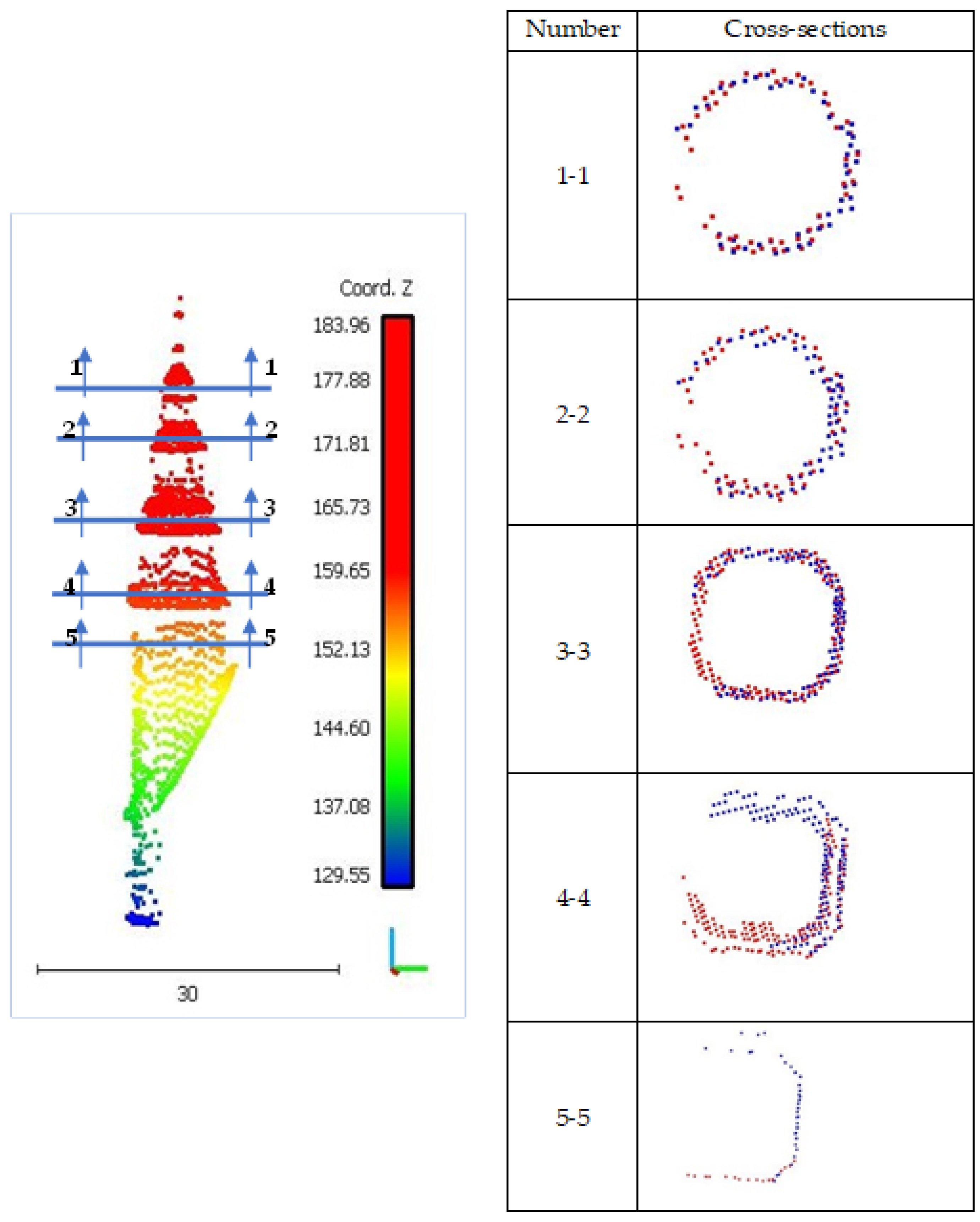
• Towers, turrets, and other ornamental structures require special modeling methods.
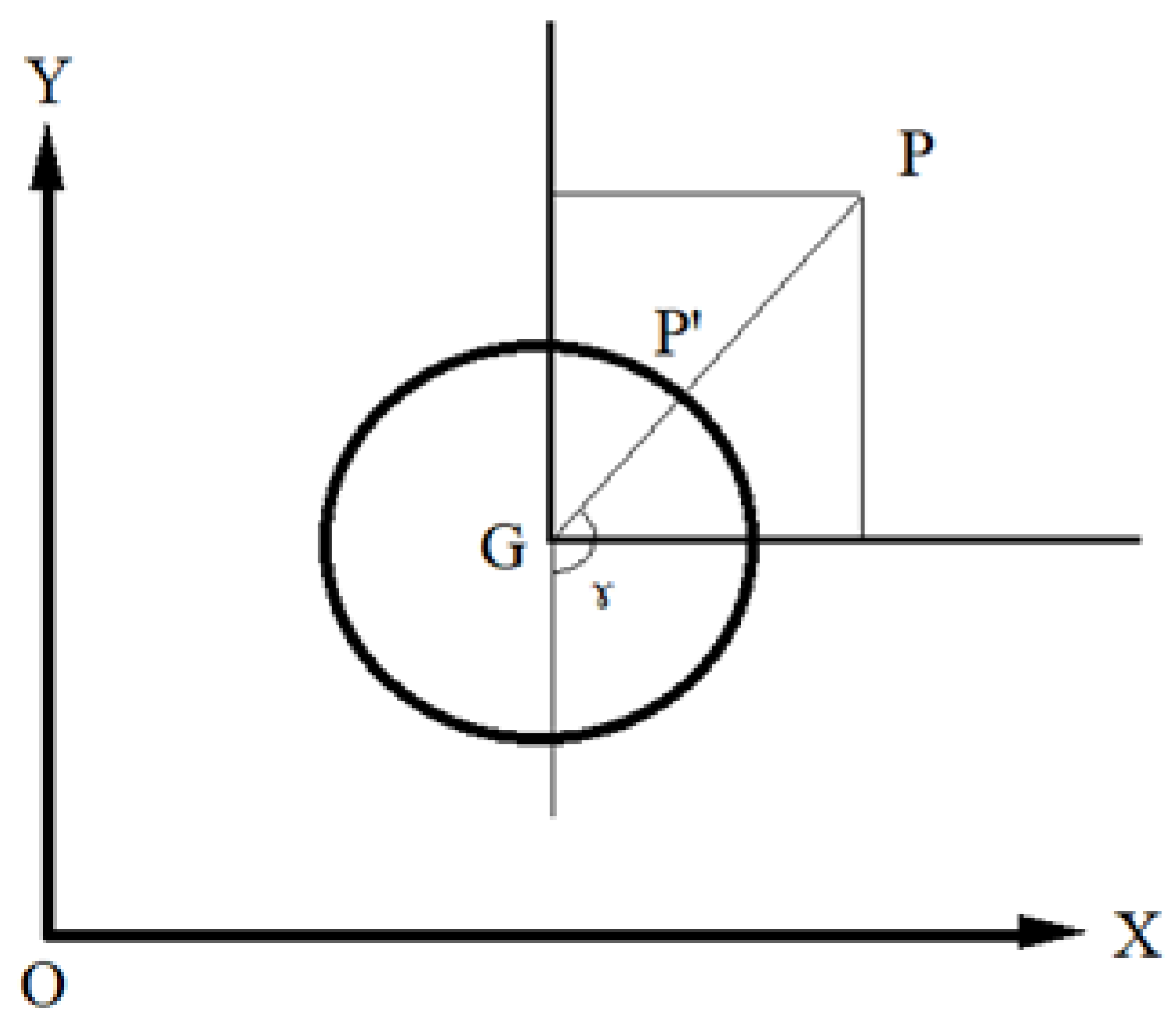
• Some of these structures can be modeled by rotating straight-line segments.
• New methods for the automatic generation of detailed building models are thus needed to ensure compliance with the CityGML 3.0 standard.

Therefore, the aim of this study was to develop an algorithm for modeling the characteristics of tall structures in buildings, represented by solids of revolution, and based on point cloud data.

3. Design Concept

The expected model that will be generated by the proposed modeling algorithm should be described first. For this purpose, an experiment was designed to assess the similarity between the envisaged model and the tower point cloud, and between the envisaged model and the tower building. The test was inspired by Tarsha Kurdi and Awrangjeb [38]. A 3D point cloud distributed irregularly on the tower’s outer surfaces can be measured by airborne laser scanning. On the one hand, the relatively low point density, irregular point distribution, accuracy of point location, presence of noisy points, and the geometric complexity of the scanned building decrease the similarity between the scanned tower and its point cloud. On the other hand, the generalization of the point cloud for calculating a 3D model decreases the similarity between the constructed model and the point cloud. Therefore, the fidelity of the constructed model decreases twice: during the scanning step and during the modeling step.

The experiment consisted of two stages. First, a 3D tower model was developed manually from the tower point cloud, without a reference to the original building image. In the first stage, the calculated model was named Model1, and it is shown in Figure 2b. Both the tower point cloud and the terrestrial image were used as inputs, to manually generate the 3D tower model. In the second stage, the calculated model was named Model2, and it is shown in Figure 2c. It should be noted that the model was generated with the use of the official Polish GIS model, which was imported to CAD and is presented as a skeleton in Figure 2c.

A comparison of the obtained tower models indicates that:

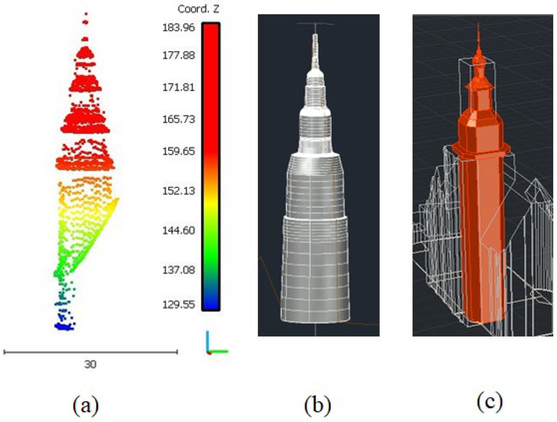
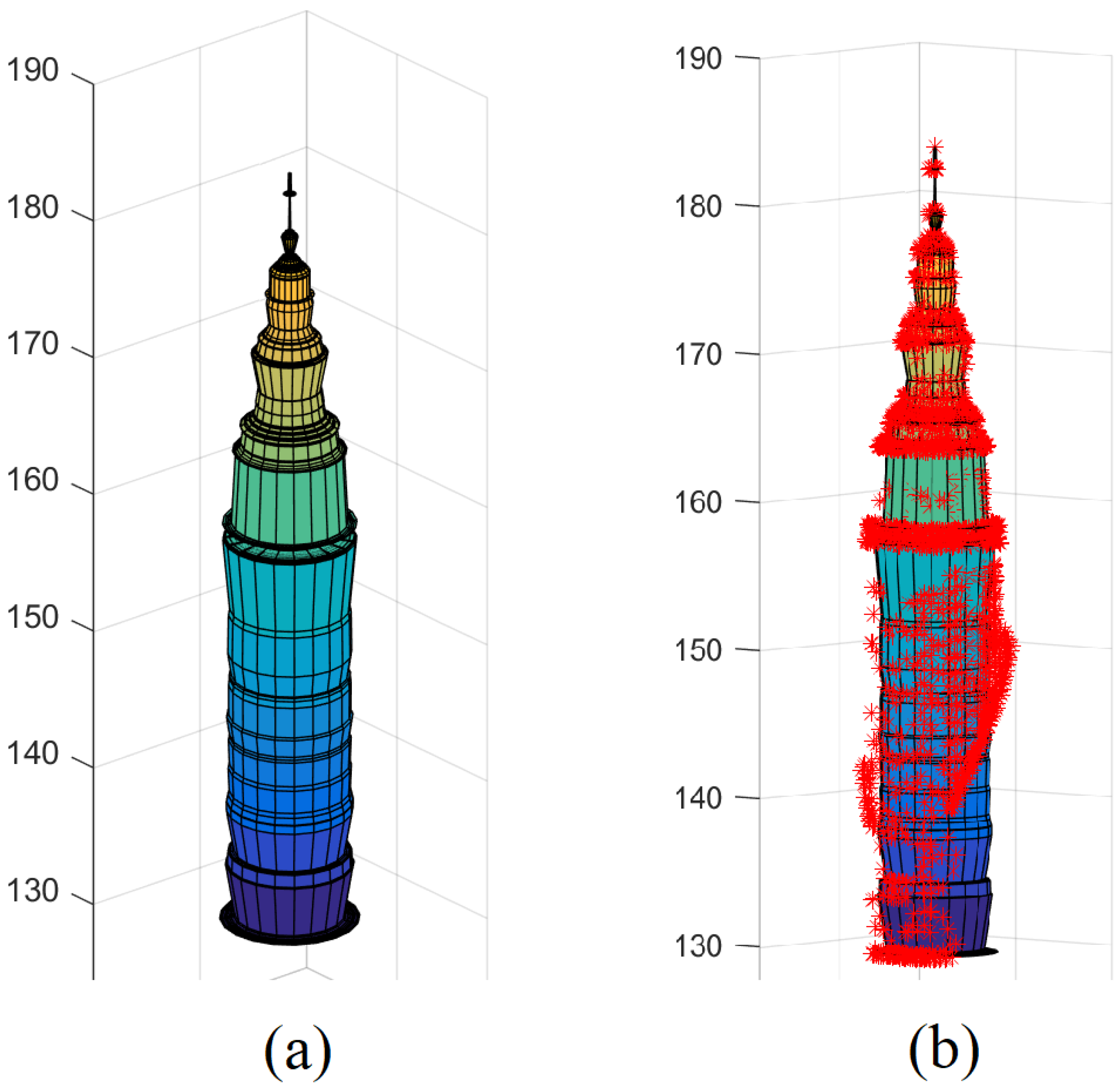
• Despite the fact that geometric details are not rendered with sufficient clarity in the point cloud, they can be identified in Model 2, but not in Model 1.
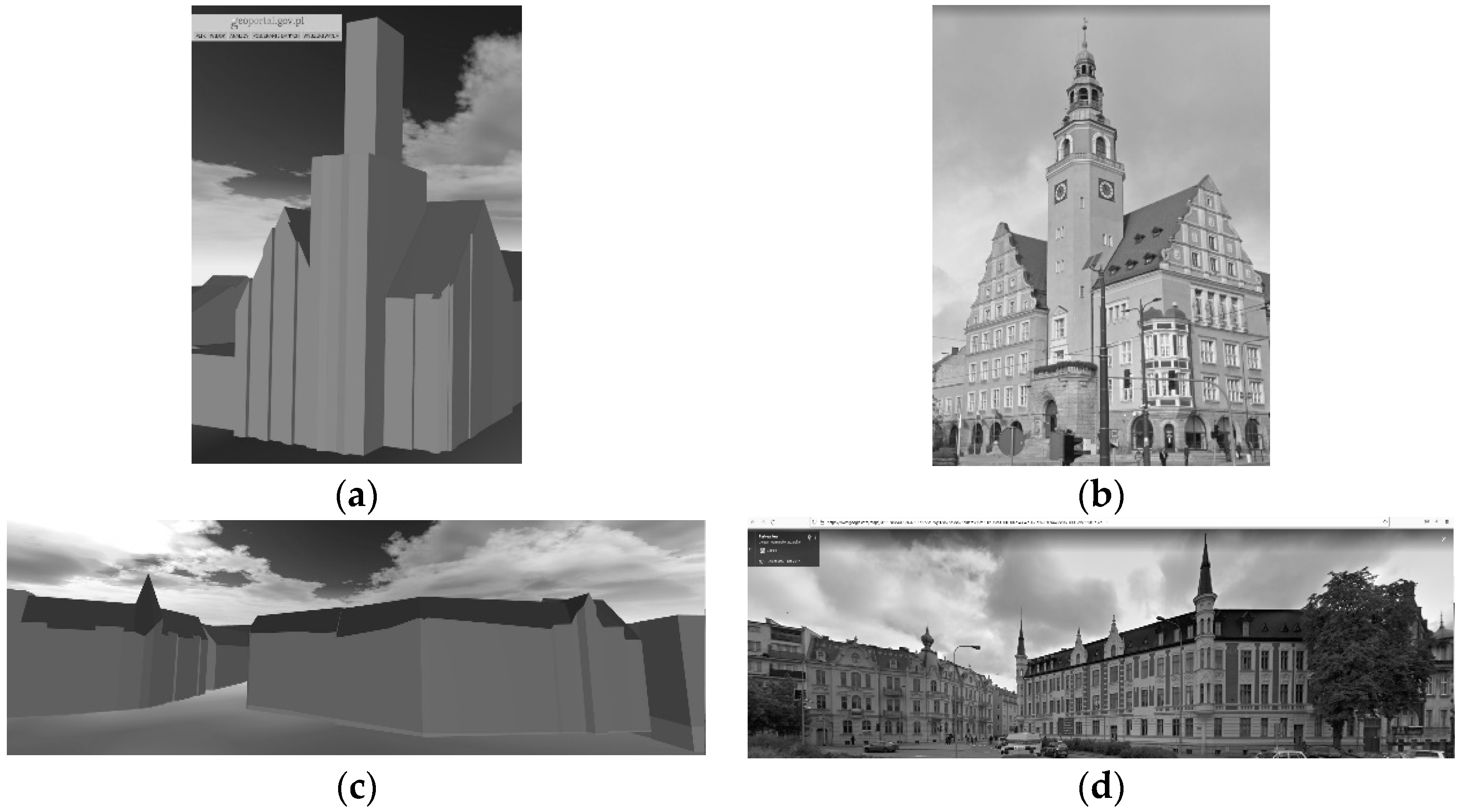
• Model 2 preserves the tower’s geometric form, which can be observed in the terrestrial image.
• Some errors in the diameters of different parts of the tower body in Model 2 result from a greater focus on the image than the point cloud.
• Model 1 renders the geometric form of different tower parts with lower accuracy, but it preserves dimensions with greater accuracy.
• Model 1 represents the point cloud more accurately than Model 2, whereas Model 2 represents the original tower more accurately than Model 1.

These observations suggest that in an automatic modeling approach, based only on an airborne LiDAR point cloud, the processing parameters and measurements are applied directly to the point cloud. Thus, the expected model will more accurately represent the point cloud describing the original building. Consequently, the constructed building may be more similar to Model 1 than Model 2.

Figure 2b indicates that the tower can be regarded as a rotational surface. The tower body is composed of five vertical parts (Figure 2); therefore, five horizontal cross-sections were calculated from the tower point cloud to verify this hypothesis, as shown in Figure 3.

The first three cross-sections are circular, but the last two are rectangular. Moreover, the point density is low in the lower part of the tower, due to airborne scanning and the presence of elements connecting the building with the tower, which is why cross-sections 4 and 5 are not complete. However, due to the tower’s architectural complexity and the fact that similar towers can be presented geometrically by rotational surfaces (as discussed in Section 4), the latter hypothesis was adopted, and tower points were modeled based on rotational surfaces.

Finally, Model 1 was built with the use of the automatic modeling approach, which relies on this strategy being applied to the point cloud, and all steps of the construction process were automated.

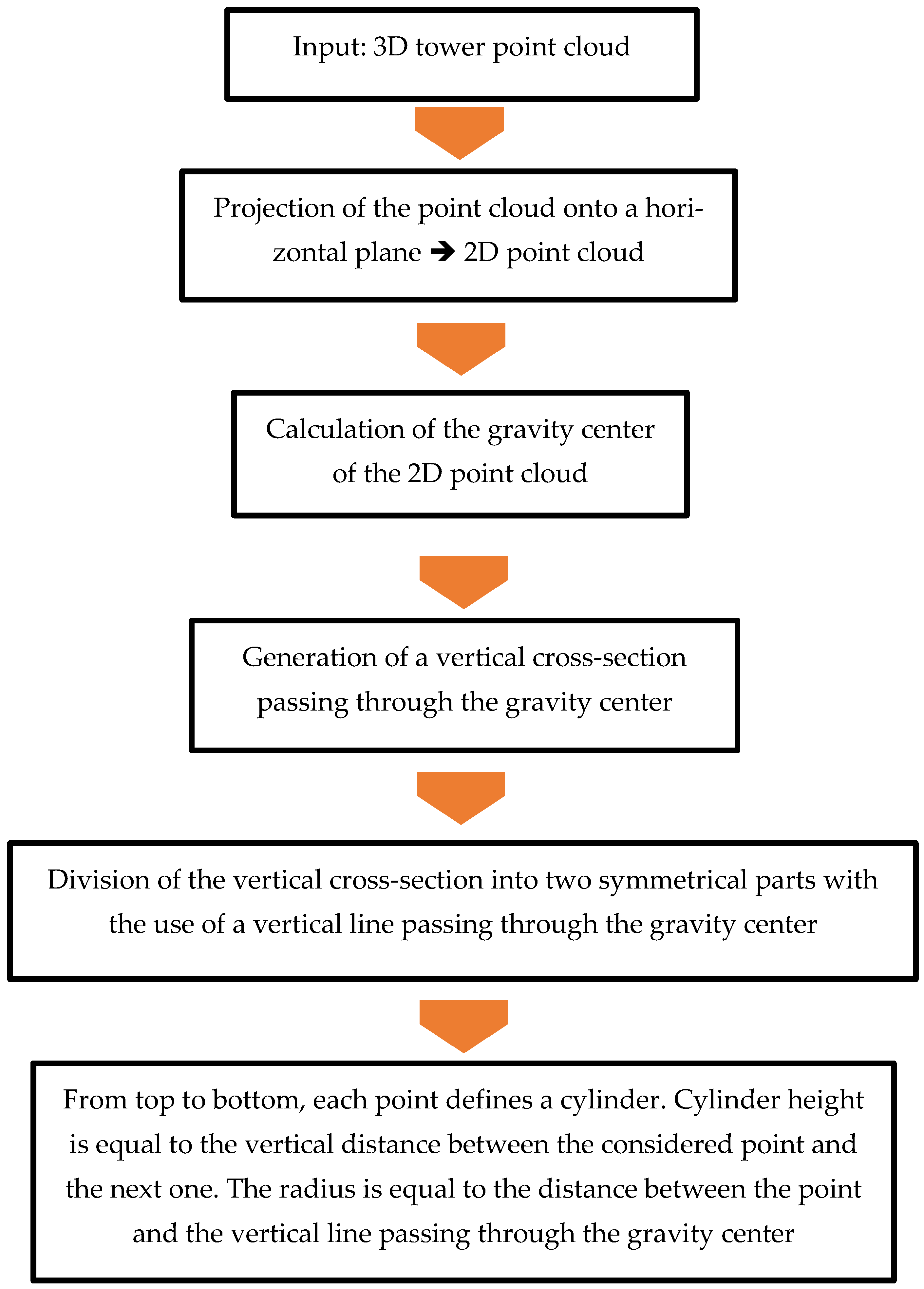
4. Proposed Modeling Approach

The suggested modeling approach was applied to the 3D airborne LiDAR point cloud of the tower. The presented algorithm was applied to automatically generate a 3D model of the scanned tower. The proposed method consists of five consecutive steps, which are presented in Figure 4. First, to calculate the tower footprint gravity center, the tower point cloud was projected onto a horizontal plane passing through the coordinate origin.

The projection on the horizontal plane OXY follows the lines parallel to the Z axis; therefore, the result is a 2D point cloud with only X and Y coordinates (the same X and Y coordinates as in 3D space). In other words, this operation could be realized by considering only the coordinates X and Y, to define a new 2D point cloud that represents the tower footprint. The elimination of the Z coordinate from the original point cloud enabled the generation of the target 2D footprint point cloud. The resulting 2D point cloud of the tower footprint is presented in Figure 5a. Due to an irregular distribution of 3D points on tower surfaces, the density of the obtained point cloud is also irregular: greater on the right side and smaller on the left side.

In the second step, the gravity center coordinates of the projected point cloud (Figure 5a) are calculated. For this purpose, the static moments of a 2D cloud are analyzed by considering the points as infinitely small elements. Therefore, static moment equations were applied to the new point cloud, to calculate the gravity center of the tower footprint (Equation (1) [39]).

The application of the static moment principle shifted the gravity center, due to an irregular point density (see the green circle in Figure 5a). The tower footprint is symmetrical, and this problem can be resolved by calculating gravity center coordinates using extreme values of X and Y coordinates (minimum and maximum), as indicated in Equation (2) (see the red circle in Figure 5a).

$$X_g=\frac{{{\displaystyle \sum }}_{i=1}^n{X}_i}{n} Y_g=\frac{{{\displaystyle \sum }}_{i=1}^n{Y}_i}{n}$$

(1)

$$X_g=minX+\frac{Xmax-Xmin}{2}, Y_g=minY+\frac{Ymax-Ymin}{2}$$

(2)

where X_g and Y_g are the coordinates of the gravity center; n is the number of points; Xi and Yi are point cloud abscissas and ordinates in OXY.

In the third step, a vertical cross-section passing through the gravity center was calculated, by identifying the points located in a slice with thickness ε around the considered vertical plane. The ε value was considered according to Equation (3) (Figure 5b).

$$\epsilon =2\times T_d T_d=\frac{1}{\sqrt{\vartheta }}$$

(3)

where ε is the thickness of the vertical cross-section slice; T_d is the mean horizontal distance between two neighboring points [29]; and θ is the point density.

In the fourth step, the symmetrical vertical cross-section was divided into two parts using the vertical line passing through the gravity center (Figure 5c). The obtained semi-cross-section represents the basic graph that revolves around the vertical line passing through the gravity center, to approximate the surface of revolution which represents the 3D tower model.

Mathematically, when a line segment is revolved around an axis, it draws a band. This band is actually a piece of a cone called the frustum of a cone. This cone could be a cylinder when the line segment is parallel to the rotating axis. Finally, from top to bottom, each point defines a cylinder, and the cylinder’s height is equal to the vertical distance between the considered point and the next one, and the radius is equal to the distance between the point and the vertical line passing through the gravity center. The analyzed semi-cross-section (Figure 5c) is not continuous and contains gaps (see the red arrow in Figure 5c). Due to the low point density and irregular point distribution, these gaps are presented by the frustums of cones connecting the two consecutive cylinders.

The 3D tower model is calculated with the use of a matrix. Three matrices were used for this purpose: X, Y, and Z (Equations (4)–(6)). These matrices represent the coordinates of rotating surface pixels and have the same number of rows and columns. The number of rows is equal to the number of points in the semi cross-section, whereas the number of columns can be selected arbitrarily, but it must be greater than seven and multiples of four added to one. In the model presented in Figure 6, the number of columns is equal to 25.

$$X=\left[\begin{array}{c}\begin{array}{c}{X}_g\\ X_g\\ X_g\end{array}\begin{array}{c} X_g+{\beta }_{1,1}\\ X_g+{\beta }_{2,1}\\ X_g+{\beta }_{3,1}\end{array} \begin{array}{c} X_g+2{\beta }_{1,2}\\ X_g+2{\beta }_{2,2}\\ X_g+2{\beta }_{3,2}\end{array}\begin{array}{c}\dots \\ \dots \\ \dots \end{array}\begin{array}{c}\dots \\ \dots \\ \dots \end{array}\begin{array}{c}{X}_g\\ X_g\\ X_g\end{array}\\ \begin{array}{c}.\\ X_g X_g+{\beta }_{n,1 } \\ \end{array}\begin{array}{c}.\\ X_g+2{\beta }_{n,2}\\ \end{array}\begin{array}{c}.\\ \dots \dots .\\ \end{array}\begin{array}{c}.\\ X_g\\ \end{array}\end{array}\right]$$

(4)

$$Y=\left[\begin{array}{c}\begin{array}{c}{Y}_1\\ Y_2\\ Y_3\end{array}\begin{array}{c} Y_1+{\alpha }_{1,1}\\ Y_2+{\alpha }_{2,1}\\ X_3+{\alpha }_{3,1}\end{array} \begin{array}{c} Y_1+2{\alpha }_{1,2}\\ Y_2+2{\alpha }_{2,2}\\ Y_3+2{\alpha }_{3,2}\end{array}\begin{array}{c}\dots \\ \dots \\ \dots \end{array}\begin{array}{c}\dots \\ \dots \\ \dots \end{array}\begin{array}{c}{Y}_1\\ Y_2\\ Y_3\end{array}\\ \begin{array}{c}.\hspace{1em}\hspace{1em} \hspace{1em}. \hspace{1em}\\ Y_n Y_N+{\alpha }_{n,1 } \\ \end{array}\begin{array}{c}.\\ Y_n+2{\alpha }_{n,2}\\ \end{array}\begin{array}{c}.\\ \dots \dots .\\ \end{array}\begin{array}{c}.\\ Y_n\\ \end{array}\end{array}\right] Z=\left[\begin{array}{c}\begin{array}{c}{Z}_1\\ Z_2\\ Z_3\end{array}\begin{array}{c}{Z}_1\\ Z_2\\ Z_3\end{array}\begin{array}{c}\dots \\ \dots \\ \dots \end{array}\begin{array}{c}\dots \\ \dots \\ \dots \end{array}\begin{array}{c}{Z}_1\\ Z_2\\ Z_3\end{array}\\ \begin{array}{c}.\\ .\\ Z_n\end{array}\begin{array}{c}.\\ .\\ Z_n\end{array}\begin{array}{c}.\\ .\\ \dots \end{array}\begin{array}{c}.\\ .\\ \dots \end{array}\begin{array}{c}.\\ .\\ Z_n\end{array}\end{array}\right]$$

(5)

$${\alpha }_{i,j}=\left(Y_g-Y_i\right)\sin (\frac{2j\pi }{m}+\frac{3\pi }{2}), {\beta }_{i,j}=\left(Y_g-Y_i\right)\cos (\frac{2j\pi }{m}+\frac{3\pi }{2})$$

(6)

where X_g and Y_g are the coordinates of the gravity center (Equation 2); X_i, Y_i, and Z_i (i = 1 to n) are the point coordinates of the semi cross-section; j = 1 to m; n is the number of points in the semi cross-section; α_i and β_i are the step values of X and Y, respectively; and m is the number of columns in matrix X.

Figure 6 presents the 3D model of the tower point cloud shown in Figure 2a. This model was constructed automatically using the described approach, based on rotational surfaces. The generated model is similar to that shown in Figure 2b, because only the tower point cloud was considered in both models. Both models represent a rotational surface and consist of five parts that are vertically superimposed. Furthermore, their dimensions are similar to the mean dimensions measured directly from the point cloud. In contrast, the model shown in Figure 2c, where both the tower point cloud and the tower image were considered, differs more considerably from the calculated model.

The suggested algorithm was implemented in MATLAB software, and the “surf (X, Y, Z)” command was used to visualize the calculated building model. However, the suggested algorithm has the following pseudocode (Algorithm 1):

Algorithm 1

Input (point cloud (X, Y, Z), m, θ) Point cloud sorted in ascending order based on Z values $X_g=minX+\frac{Xmax-Xmin}{2}$  $Y_g=minY+\frac{Ymax-Ymin}{2}$  $T_d=\frac{1}{\sqrt{\vartheta }}$ i = find (X > Xg − Td and X < Xg + Td and Y ≤ Yg) SCS = [Y(i), Z(i)] for i = 1 to length (SCS), Step = 1     for j = 0 to m, Step = 1        Zb (i, j+1) = SCS (i, 2)        Xb (i, j+1) = Xg + (Yg − SCS (i, 1)) × cos($\frac{3\times \pi }{2}+\frac{2\times j\times \pi }{m}$)        Yb (i, j+1) = Xg + (Yg − SCS (i, 1)) × sin($\frac{3\times \pi }{2}+\frac{2\times j\times \pi }{m}$)     Next j Next i Surf (X, Y, Z)

Where SCS is the list of semi-cross-section points; Surf is the 3D visualization function; X_b, Y_b, and Z_b are the three matrices of the building model (Equations (4) and (5)).

In the previous pseudocode, the suggested algorithm was very short and simple. The algorithm outputs three matrices that can be exported in raster or vector format. The datasets used in the suggested approach will be presented in the next section. The remaining results will be discussed and the accuracy of the modeling process will be estimated in Section 6.

5. Datasets

The Polish SDI was developed by the Head Office of Geodesy and Cartography, and constitutes a data source that is widely used in research. ALS data from LiDAR measurements conducted in 2018 (12 point/m²), as well as LOD2 3D building models generated in the CityGML 2.0 standard, were selected from SDI resources for the needs of the study.

The 3D building models were generated by compiling three data sources: 2D building contours from the Database of Topographic Objects in 1:10 000 scale, LiDAR data (building class), and the Digital Terrain Model (DTM) with a mesh size of 1 m. Buildings were modeled based on 2D building contours. The height of building contours was determined based on the minimum height of building contour vertices in the DTM dataset. The 3D building models were downloaded from the SDI, as individual vector files presenting roof planes, building walls, and 2D building contours.

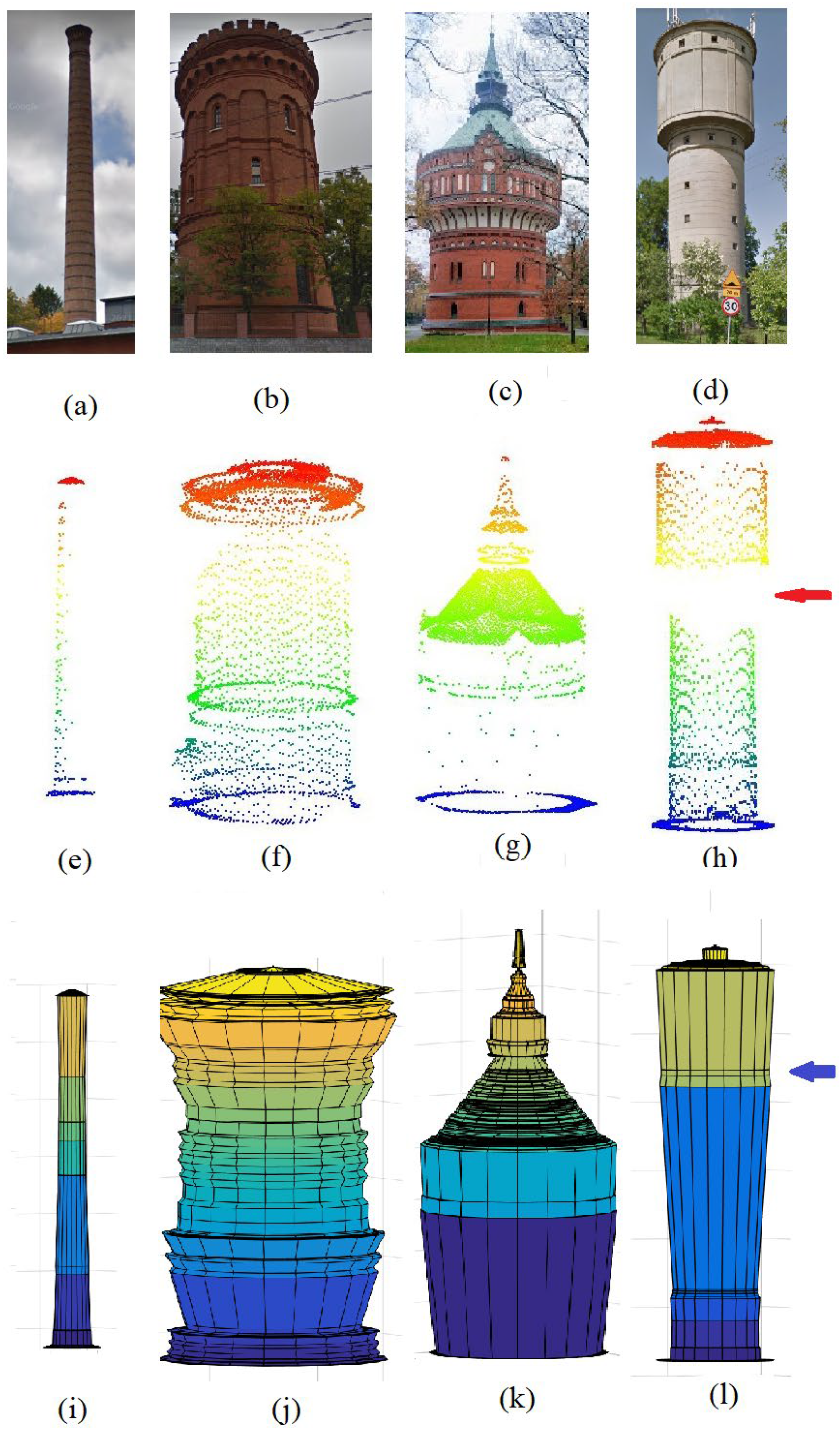
The most characteristic buildings in Olsztyn, including the Olsztyn City Hall with an ornamental tower (Figure 1a,b), a building with a chimney (Figure 7a), and water towers (Figure 7b), were selected for the study. Two water towers with characteristic shapes, located in the cities of Bydgoszcz (Figure 7c) and Siedlce (Figure 7d), were additionally selected. ALS data were obtained from SDI resources.

6. Results, Accuracy Estimation, and Discussion

In the literature, the accuracy of 3D building models generated based on LiDAR data can be estimated using two approaches. In the first approach, the generated model is compared with the reference model [15,40,41,42]. In the second approach, a LiDAR point cloud is the reference model [15,38,43,44,45]. In the second approach, the accuracy is estimated by calculating the distances between the 3D model and the point cloud. In the present study, the reference model was the building point cloud. To estimate the accuracy of the generated model, the point cloud is superimposed onto the built model, and the distances between cloud points and the model are calculated. The point cloud is superimposed onto the 3D tower model in Figure 6b. A histogram of the distances between cloud points and the generated tower model (see Figure 6b) is shown in Figure 8. Figure 8 shows that a high percentage of points fit the constructed tower model accurately, and the distances between the points and the model are less than 0.30 m. A distance of less than 0.35 m is regarded as acceptable. The accuracy of altimetry measurements, the texture of building surfaces and ornaments, and the presence of noise shift cloud points around the mean building surfaces. Moreover, some parts of the building do not support the hypothesis postulating that the building is represented by a rotational surface. For example, the lower part of the tower in Figure 3 is not exactly a rotational surface.

In addition to the point cloud presented in Figure 2a, four different tower point clouds were assessed, to analyze the accuracy of the models developed with the suggested approach. The images, the point cloud, and the constructed models of four tower point clouds are presented in Figure 7. The total number of points, the number of points that deviate from the model within the interval (0, 0.3 m), the number of points with deviations greater than 0.3 m, and the standard deviation of the distances from the constructed model are presented in

Table 1. Standard deviations and the number of points that deviate from the tower model within the specified intervals.

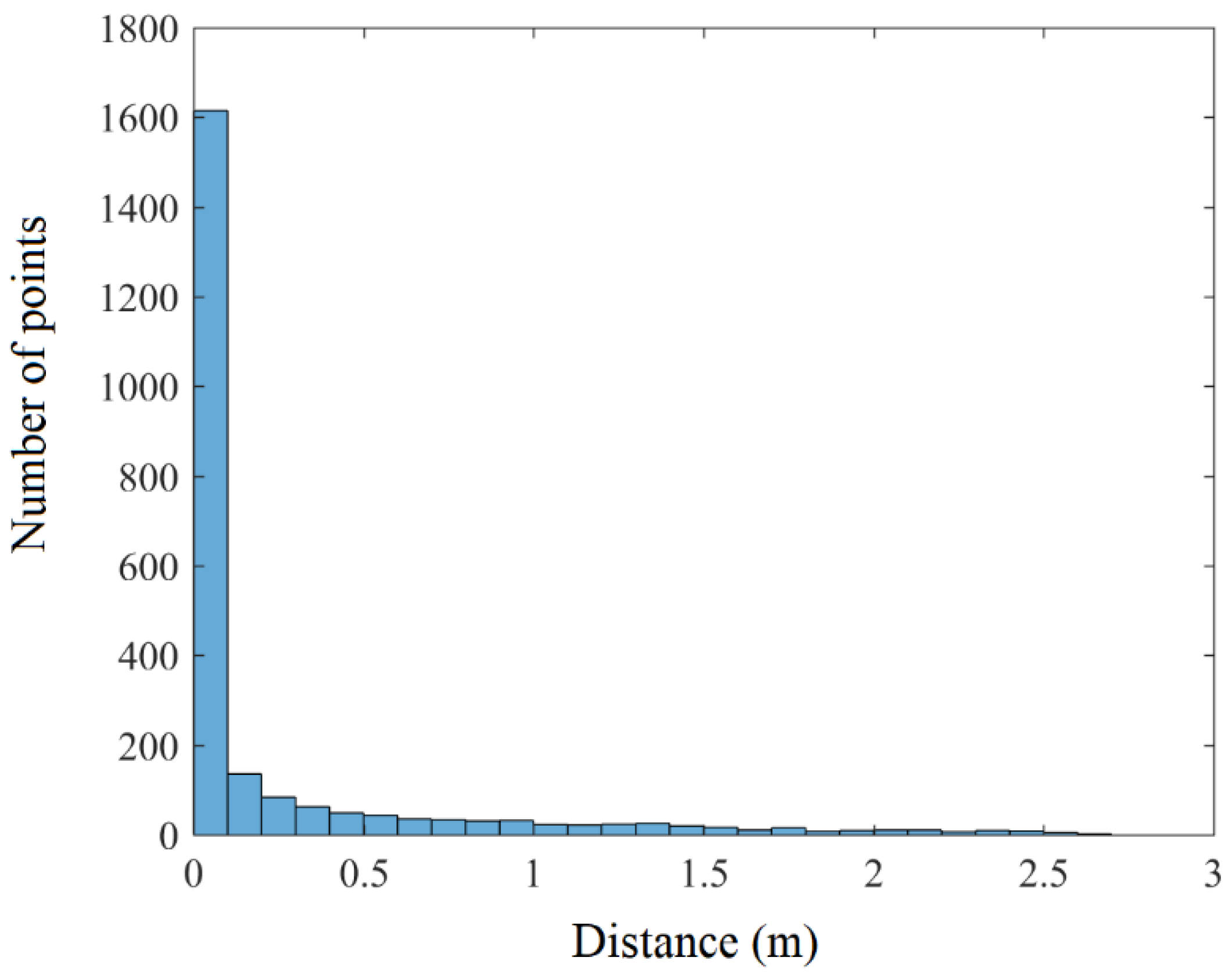
Tower Number Name–City	Number of Points	Number of Points		σ (m)
		Dist ϵ (0, 0.3 m)	Dist > 0.3 m
1 Olsztyn City Hall	2330	1833	497	0.49
2 Building with a chimney in Olsztyn	330	244	86	0.9
3 Water tower in Olsztyn	4974	2217	2757	0.84
4 Water tower in Bydgoszcz	5500	5246	254	0.21
5 Water tower in Siedlce	4811	3825	986	1.4

Dist: deviation between a point and the constructed model; σ: standard deviation of the distance between the cloud point and the tower model.

.

It should be noted that the same approach was used to calculate the values presented in Table 1 and the histogram in Figure 8. Hence, the tower point cloud was superimposed onto the calculated model, and the deviation of each point from the constructed model was calculated. This operation was performed to calculate the deviation for each point. A histogram of deviations is presented in Figure 8. The calculated deviations were analyzed, and the results are presented in Table 1.

To calculate the deviation of a given Point P (X_p, Y_p, Z_p) in Figure 9, the Z coordinate was used to determine the point’s location in matrix Z in Equation 5. The point can have three locations. In the first case, if the point is located in a row where Z_p = Z_i (I = 1 to n), the deviation can be calculated according to Equation (7) (as shown in Figure 9).

$$div=\sqrt{{\left(X_p-X_g\right)}^2+{\left(Y_p-Y_g\right)}^2}-Y_g+Y_i$$

(7)

In the second case, if Point P is located between two rows, the deviation is calculated for each of the two rows, and the final deviation is estimated for the last two values. In the third case, if Point P is located outside matrix Z values (up or down), it is considered a noisy point and neglected.

In Figure 9, distance P P’ represents deviation, and distance P’G represents the radius of rotation, which equals Y_i − Y_g. In Equation (6), angle ɤ equals ((2.j.π)/m). It should be noted that the deviation can be negative or positive, depending on the point’s location in the calculated model. The deviation is negative if the point is located inside the model, and positive if the point is located outside the calculated model. Standard deviation always has a positive value.

In Table 1, tower No. 1 is the tower shown in Figure 2, whereas towers No. 2, 3, 4, and 5 are the towers shown in Figure 7, in the same order.

In Table 1, Tower 5 has the greatest standard deviation (σ = 1.4 m). This tower consists of two main parts, separated by a step. The points located down the step are not shown (see the red arrow in Figure 7h) because the object was scanned from an aerial view, and the missed points are located within the hidden area. In fact, the suggested modeling algorithm replaces the missing points with the frustum of a cone, which is why the obtained model was deformed in the hidden area (see the blue arrow in Figure 7l). Despite a high standard deviation, most points fit the calculated model.

In building No. 3, the number of points that well fit the tower model is almost equal to the number of points with a deviation greater than 0.3 m. In Figure 7b, the deviations can be attributed to the highly ornamental building facades. From another viewpoint, the reasonable standard deviation (σ = 0.84 m) confirms this result. Tower No. 2 has a simple architectural design, and the deviation is below the minimal value of standard deviation (σ = 0.21 m).

The suggested approach has certain limitations. The proposed algorithm assumes that building facades are completely covered by LiDAR points. In fact, this hypothesis may not always be valid. Therefore, when facade points disappear for whatever reason, the analyzed building details will also disappear. Moreover, the discussed method is very sensitive to noisy points, which can substantially deform the building model. Fortunately, this issue can be resolved by considering point deviation values in addition to building symmetry. Some geometrical forms create hidden areas that cannot be accessed by laser pulses, such as the building shown in Figure 7d. These hidden areas may produce distortions in the calculated building model.

It should be noted that most algorithms for modeling buildings based on LiDAR data suggested in the literature are model-driven or data-driven approaches [39]. In these approaches, the concept of a building model relies on the assumption that the building consists of connected facets that are described by neighborhood relationships. The connections between these facets form facet borders and vertices. A comparison of the proposed modeling approach and the approaches suggested in the literature indicates that the developed algorithm does not belong to the last two modeling approaches, because the building concept differs entirely from the modeling approaches where one building is represented by three matrices that describe the building’s geometric form.

However, modeling algorithms should be compared based on their performance. Therefore, three selected approaches were compared with the proposed algorithm in

Table 2. Accuracy of the proposed approach and previous algorithms.

Approach	Standard Deviation
Proposed algorithm	0.21 m to 1.41 m
Kulawiak [3]	0.29 m to 2.36 m
Ostrowski et al. [15]	<0.3 m to >1 m
Jung and Sohn [42]	0.05 m to >3 m

. In Table 2, standard deviation was used to estimate the accuracy of the generated model. Despite differences in the architectural complexity of the target buildings in the compared approaches, the accuracy of the suggested algorithm is still acceptable.

To conclude, the suggested approach paves the way to developing new and general modeling methods based on a matrix representation of buildings with both simple and complex architectural features. In the future, the proposed model could be further improved by integrating point deviations and improving the model’s fidelity to the original point cloud.

7. Conclusions

This article proposes a methodology for automating the modeling of buildings with ornamental turrets and towers based on LiDAR data. The proposed modeling procedure was based directly on a point cloud. A vertical axis was generated from a LIDAR data subset describing a tower. It was assumed that the tower was symmetrical about its axis. A cross-section was introduced to the point cloud, with a plane passing through the axis, which produced a vertical cross-section. The vertical cross-section was used to build a solid of revolutions, as the 3D model of the tower. The modeling algorithm relied on a matrix to generate the building model in a mathematical form.

Five tower point clouds were used to evaluate the accuracy of the suggested method. Hence, the deviation of points representing the obtained model was calculated, in addition to the standard deviation. Despite the algorithm’s overall efficacy, it had three main limitations. The tower was not covered by LiDAR data in its entirety. Moreover, some geometric forms may generate hidden areas that can produce deformations in the model. Moreover, the suggested algorithm is sensitive to the presence of noisy points. However, facade ornaments, an insufficient accuracy of LiDAR data, and noisy points significantly decreased the accuracy of the generated model. In the future, the building model can be enhanced by considering points with considerable deviations. The matrix form of the proposed algorithm facilitates local enhancements. In addition to the matrix, a vertical cross-section can also be applied to develop a new approach for modeling buildings, regardless of the level of architectural complexity. Finally, additional data, such as aerial or terrestrial imagery, could be incorporated into the proposed modeling approach, to increase the model’s fidelity to the original building.

References

- Dong, Z.; Liang, F.; Yang, B.; Xu, Y.; Zang, Y.; Li, J.; Stilla, U. Registration of large-scale terrestrial laser scanner point clouds: A review and benchmark. ISPRS J. Photogramm. Remote Sens. 2020, 163, 327–342. [Google Scholar] [CrossRef]
- Cheng, L.; Chen, S.; Liu, X.; Xu, H.; Wu, Y.; Li, M.; Chen, Y. Registration of laser scanning point clouds: A review. Sensors 2018, 18, 1641. [Google Scholar] [CrossRef] [PubMed]
- Kulawiak, M. A cost-effective method for reconstructing city-building 3D models from sparse lidar point clouds. Remote Sens. 2022, 14, 1278. [Google Scholar] [CrossRef]
- Yan, W.Y.; Shaker, A.; El-Ashmawy, N. Urban land cover classification using airborne LiDAR data: A review. Remote Sens. Environ. 2015, 158, 295–310. [Google Scholar] [CrossRef]
- Shan, J.; Toth, C.K. Topographic Laser Ranging and Scanning: Principles and Processing, 2nd ed.; Taylor & Francis Group; CRC Press: Boca Raton, FL, USA, 2018. [Google Scholar] [CrossRef]
- Xu, Y.; Stilla, U. Towards Building and Civil Infrastructure Reconstruction from Point Clouds: A Review on Data and Key Techniques. IEEE J. Sel. Top. Appl. Earth Obs. Remote Sens. 2021, 14, 2857–2885. [Google Scholar] [CrossRef]
- Tarsha Kurdi, F.; Awrangjeb, M.; Munir, N. Automatic filtering and 2D modeling of LiDAR building point cloud. Trans. GIS 2021, 25, 164–188. [Google Scholar] [CrossRef]
- Amakhchan, W.; Kurdi, F.T.; Gharineiat, Z.; Boulaassal, H.; Kharki, O.E. Automatic Filtering of LiDAR Building Point Cloud Using Multilayer Perceptron Neuron Network. In Proceedings of the Conference: 3rd International Conference on Big Data and Machine Learning (BML22’), Istanbul, Turkey, 21–31 May 2022. [Google Scholar]
- Wen, C.; Yang, L.; Li, X.; Peng, L.; Chi, T. Directionally constrained fully convolutional neural network for airborne LiDAR point cloud classification. ISPRS J. Photogramm. Remote Sens. 2020, 162, 50–62. [Google Scholar] [CrossRef]
- Tarsha Kurdi, F.; Amakhchan, W.; Gharineiat, Z. Random Forest machine learning technique for automatic vegetation detection and modeling in LiDAR data. Int. J. Environ. Sci. Nat. Resour. 2021, 28, 556234. [Google Scholar] [CrossRef]
- Maltezos, E.; Doulamis, A.; Doulamis, N.; Ioannidis, C. Building extraction from LiDAR data applying deep convolutional neural networks. IEEE Geosci. Remote Sens. Lett. 2018, 16, 155–159. [Google Scholar] [CrossRef]
- Wang, X.; Luo, Y.P.; Jiang, T.; Gong, H.; Luo, S.; Zhang, X.W. A new classification method for LIDAR data based on unbalanced support vector machine. In Proceedings of the 2011 International Symposium on Image and Data Fusion, Tengchong, China, 9–11 August 2011; pp. 1–4. [Google Scholar] [CrossRef]
- Yuan, J. Learning building extraction in aerial scenes with convolutional networks. IEEE Trans. Pattern Anal. Mach. Intell. 2017, 40, 2793–2798. [Google Scholar] [CrossRef]
- Chio, S.H.; Lin, T.Y. The establishment of 3D LOD2 objectivization building models based on data fusion. J. Photogramm. Remote Sens. 2021, 26, 57–73. Available online: https://www.csprs.org.tw/Temp/202106-26-2-57-73.pdf\ (accessed on 16 September 2022).
- Ostrowski, W.; Pilarska, M.; Charyton, J.; Bakuła, K. Analysis of 3D building models accuracy based on the airborne laser scanning point clouds. In International Archives of the Photogrammetry, Remote Sensing & Spatial Information Sciences; ISPRS: Vienna, Austria, 2018; p. 42. Available online: https://www.int-arch-photogramm-remote-sens-spatial-inf-sci.net/XLII-2/797/2018/#:~:text=https%3A//doi.org/10.5194/isprs%2Darchives%2DXLII%2D2%2D797%2D2018%2C%202018 (accessed on 16 September 2022).
- Zhang, K.; Yan, J.; Chen, S.C. A framework for automated construction of building models from airborne Lidar measurements. In Topographic Laser Ranging and Scanning: Principles and Processing, 2nd ed.; Shan, J., Toth, C.K., Eds.; Taylor & Francis Group; CRC Press: Boca Raton, FL, USA, 2018; pp. 563–586. [Google Scholar]
- Van Oosferom, P.J.M.; Broekhuizen, M.; Kalogianni, E. BIM models as input for 3D land administration systems for apartment registration. In Proceedings of the 7th International FIG Workshop on 3D Cadastres, New York, NY, USA, 11–13 October 2021; International Federation of Surveyors (FIG): Copenhagen, Denmark, 2021; pp. 53–74. Available online: https://research.tudelft.nl/en/publications/bim-models-as-input-for-3d-land-administration-systems-for-apartm; https://www.proquest.com/results/883F9FCF559E442EPQ/false?accountid=14884\ (accessed on 16 September 2022).
- Beil, C.; Ruhdorfer, R.; Coduro, T.; Kolbe, T.H. Detailed streetspace modeling for multiple applications: Discussions on the proposed CityGML 3.0 transportation model. ISPRS Int. J. Geo-Inf. 2020, 9, 603. [Google Scholar] [CrossRef]
- Biljecki, F.; Lim, J.; Crawford, J.; Moraru, D.; Tauscher, H.; Konde, A.; Adouane, K.; Lawrence, S.; Janssen, P.; Stouffs, R. Extending CityGML for IFC-sourced 3d city models. Autom. Constr. 2021, 121, 103440. [Google Scholar] [CrossRef]
- Jayaraj, P.; Ramiya, A.M. 3D CityGML building modeling from lidar point cloud data. In The International Archives of Photogrammetry, Remote Sensing and Spatial Information Sciences; Gottingen Tom XLII-5; Copernicus GmbH: Gottingen, Germany, 2018; pp. 175–180. Available online: https://www.proquest.com/opeview/47e1bca8fac2930d4be04e70741e905f/1 (accessed on 20 September 2022). [CrossRef]
- Lukač, N.; Žalik, B. GPU-based roofs’ solar potential estimation using LiDAR data. Comput. Geosci. 2013, 52, 34–41. [Google Scholar] [CrossRef]
- Beil, C.; Kutzner, T.; Schwab, B.; Willenborg, B.; Gawronski, A.; Kolbe, T.H. Integration of 3D point clouds with semantic 3D City Models—providing semantic information beyond classification. In ISPRS Annals of the Photogrammetry, Remote Sensing and Spatial Information Sciences; Gottingen Tom VIII-4/W2-2021; Copernicus GmbH: Gottingen, Germany, 2021; pp. 105–112. Available online: https://www.proquest.com/openview/6c8a777f6d7c8645edb6dad807b248aa/1?pq-origsite=gscholar&cbl=2037681 (accessed on 16 September 2022). [CrossRef]
- Chaturvedi, K.; Matheus, A.; Nguyen Son, H.; Kolbe, H. Securing spatial data infrastructures for distributed smart city applications and services. Future Gener. Comput. Syst. 2019, 101, 723–736. [Google Scholar] [CrossRef]
- Kutzner, T.; Chaturvedi, K.; Kolbe, T.H. CityGML 3.0: New functions open up new applications. PFG J. Photogramm. Remote Sens. Geoinf. Sci. 2020, 88, 43–61. [Google Scholar] [CrossRef]
- Shirinyan, E.; Petrova-Antonova, D. Modeling buildings in CityGML LOD1: Building parts, terrain intersection curve, and address features. ISPRS Int. J. Geo-Inf. 2022, 11, 166. [Google Scholar] [CrossRef]
- Biljecki, F.; Ledoux, H.; Stoter, J. Generation of multi-LOD 3D city models in CityGML with the procedural modelling engine random3dcity, ISPRS ann. Photogramm. Remote Sens. Spatial Inf. Sci. 2016, IV-4/W1, 51–59. [Google Scholar] [CrossRef]
- Gilani, S.A.N.; Awrangjeb, M.; Lu, G. Segmentation of airborne point cloud data for automatic building roof extraction. GISci. Remote Sens. 2018, 55, 63–89. [Google Scholar] [CrossRef]
- Chen, D.; Zhang, L.; Mathiopoulos, P.; Huang, X. A methodology for automated segmentation and reconstruction of urban 3-D buildings from ALS point clouds. IEEE J. Sel. Top. Appl. Earth Obs. Remote Sens. 2014, 7, 4199–4217. [Google Scholar] [CrossRef]
- Dey, E.K.; Tarsha Kurdi, F.; Awrangjeb, M.; Stantic, B. Effective selection of variable point neighbourhood for feature point extraction from aerial building point cloud data. Remote Sens. 2021, 13, 1520. [Google Scholar] [CrossRef]
- Dong, Y.; Hou, M.; Xu, B.; Li, Y.; Ji, Y. Ming and Qing dynasty official-style architecture roof types classification based on the 3D point cloud. ISPRS Int. J. Geo-Inf. 2021, 10, 650. [Google Scholar] [CrossRef]
- Awrangjeb, M.; Gilani, S.A.N.; Siddiqui, F.U. An effective datadriven method for 3-d building roof reconstruction and robust change detection. Remote Sens. 2018, 10, 1512. [Google Scholar] [CrossRef]
- Tarsha Kurdi, F.; Awrangjeb, M.; Munir, N. Automatic 2D modelling of inner roof planes boundaries starting from Lidar data. In Proceedings of the 14th 3D GeoInfo 2019, Singapore, 26–27 September 2019. [Google Scholar] [CrossRef]
- Tarsha Kurdi, F.; Gharineiat, Z.; Campbell, G.; Dey, E.K.; Awrangjeb, M. Full series algorithm of automatic building extraction and modeling from LiDAR data. In Proceedings of the Digital Image Computing: Techniques and Applications (DICTA), Gold Coast, Australia, 29 November–1 December 2021; pp. 1–8. [Google Scholar] [CrossRef]
- Dey, E.K.; Awrangjeb, M.; Tarsha Kurdi, F.; Stantic, B. Building boundary point extraction from LiDAR point cloud data. In Proceedings of the 2021 Digital Image Computing: Techniques and Applications (DICTA), Gold Coast, Australia, 29 November–1 December 2021; pp. 1–8. [Google Scholar] [CrossRef]
- Huang, J.; Stoter, J.; Peters, R.; Nan, L. City3D: Large-scale building reconstruction from airborne LiDAR point clouds. Remote Sens. 2022, 14, 2254. [Google Scholar] [CrossRef]
- Borisov, M.; Radulovi, V.; Ilić, Z.; Petrovi, V.; Rakićević, N. An automated process of creating 3D city model for monitoring urban infrastructures. J. Geogr. Res. 2022, 5. Available online: https://ojs.bilpublishing.com/index.php/j (accessed on 16 September 2022). [CrossRef]
- Tarsha Kurdi, F.; Gharineiat, Z.; Campbell, G.; Awrangjeb, M.; Dey, E.K. Automatic filtering of LiDAR building point cloud in case of trees associated to building roof. Remote Sens. 2022, 14, 430. [Google Scholar] [CrossRef]
- Tarsha Kurdi, F.; Awrangjeb, M. Comparison of LiDAR building point cloud with reference model for deep comprehension of cloud structure. Can. J. Remote Sens. 2020, 46, 603–621. [Google Scholar] [CrossRef]
- Tarsha Kurdi, T.; Landes, T.; Grussenmeyer, P.; Koehl, M. Model-driven and data-driven approaches using Lidar data: Analysis and comparison. In Proceedings of the ISPRS Workshop, Photogrammetric Image Analysis (PIA07), Munich, Germany, 19–21 September 2007; International Archives of Photogrammetry, Remote Sensing and Spatial Information Systems: Stuttgart, Germany, 2007; Volume XXXVI, pp. 87–92, ISSN 1682-1750. [Google Scholar]
- Cheng, L.; Zhang, W.; Zhong, L.; Du, P.; Li, M. Framework for evaluating visual and geometric quality of three-dimensional models. IEEE J. Sel. Top. Appl. Earth Obs. Remote Sens. 2015, 8, 1281–1294. [Google Scholar] [CrossRef]
- Rottensteiner, F.; Clode, S. Building and road extraction from Lidar data. In Topographic Laser Ranging and Scanning: Principles and Processing, 2nd ed.; Shan, J., Toth, C.K., Eds.; Taylor & Francis Group; CRC Press: Boca Raton, FL, USA, 2018; pp. 485–522. [Google Scholar]
- Jung, J.; Sohn, G. Progressive modeling of 3D building rooftops from airborne Lidar and imagery. In Topographic Laser Ranging and Scanning: Principles and Processing, 2nd ed.; Shan, J., Toth, C.K., Eds.; Taylor & Francis Group; CRC Press: Boca Raton, FL, USA, 2018; pp. 523–562. [Google Scholar]
- Dorninger, P.; Pfeifer, N. A comprehensive automated 3D approach for building extraction, reconstruction, and regularization from airborne laser scanning point clouds. Sensors 2008, 8, 7323–7343. [Google Scholar] [CrossRef]
- Sampath, A.; Shan, J. Segmentation and reconstruction of polyhedral building roofs from aerial Lidar point clouds. IEEE Trans. Geosci. Remote Sens. 2010, 48, 1154–1567. [Google Scholar] [CrossRef]
- Park, S.Y.; Lee, D.G.; Yoo, E.J.; Lee, D.C. Segmentation of Lidar data using multilevel cube code. J. Sens. 2019, 2019, 4098413. [Google Scholar] [CrossRef]