
Image-Based Classification of Double-Barred Beach States Using a Convolutional Neural Network and Transfer Learning


Abstract
1. Introduction
2. Field Sites and Datasets
2.1. Field Sites
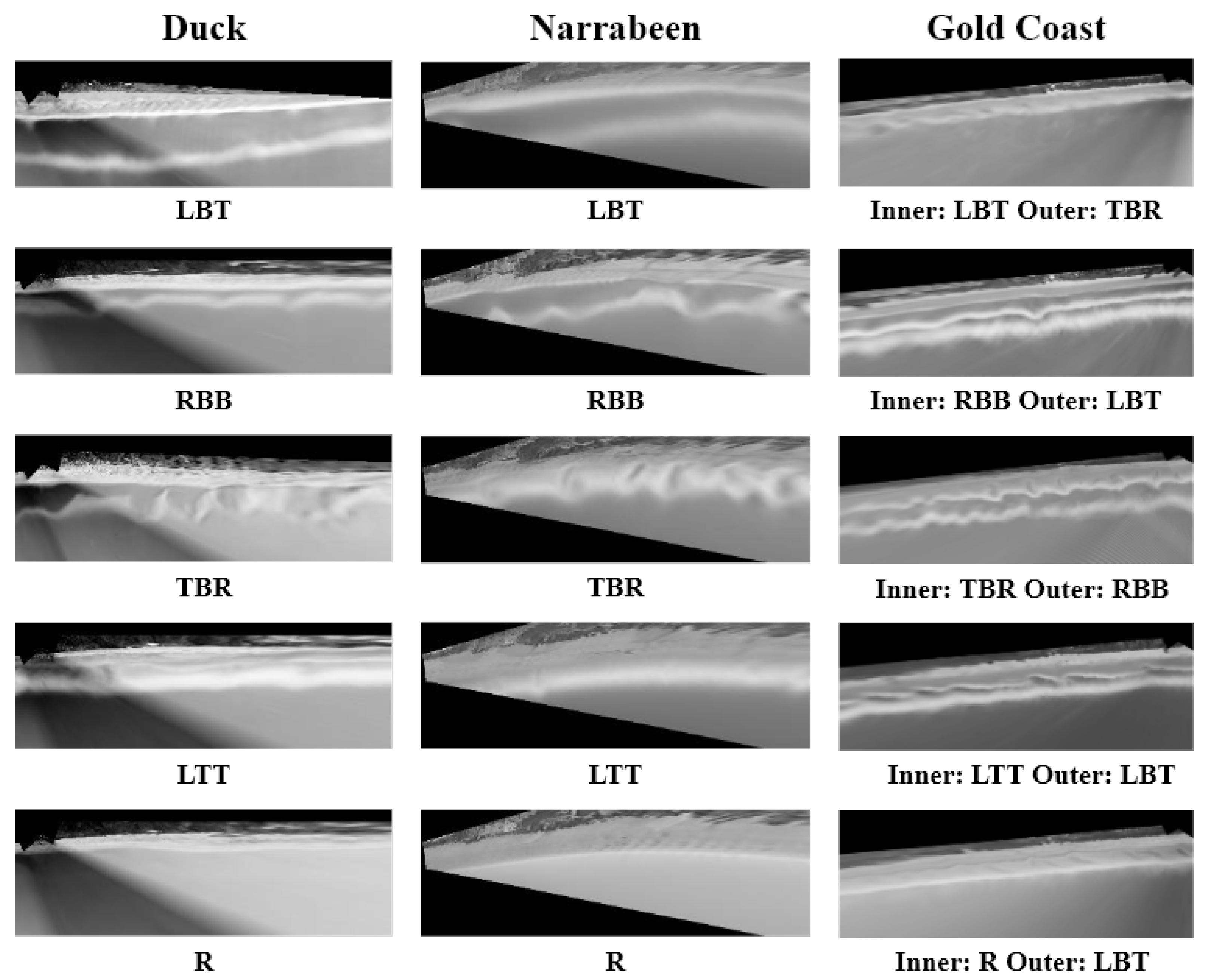
2.1.1. Duck
2.1.2. Narrabeen-Collaroy
2.1.3. Gold Coast
2.2. Datasets
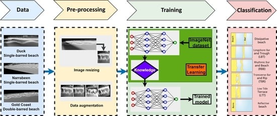
3. Methodology
- Collect the datasets;
- Model initialization;
- Prepare the data;
- Train models with various datasets;
- Test the models on various locations;
- Report the performance for each test.
3.1. Model Initialization
3.1.1. ResNet50
3.1.2. Training Protocols and Transfer Learning
3.2. Data Preparation
4. Experimental Setup
4.1. Experiment 1: Single-Bar Beach Models
4.2. Experiment 2: Double-Bar Beach Models
4.3. Performance Measures
- True Positive (TP): TP denotes the number of cases in which the CNN classified Yes correctly.
- True Negative (TN): TN signifies the number of cases the CNN classified No correctly.
- False Positive (FP): FP is the number of cases we classified Yes where the true class is No.
- False Negative (FN): FN denotes the number of cases the CNN classified No where the true class is Yes.
5. Results
5.1. Single-Bar Beach Models Performances
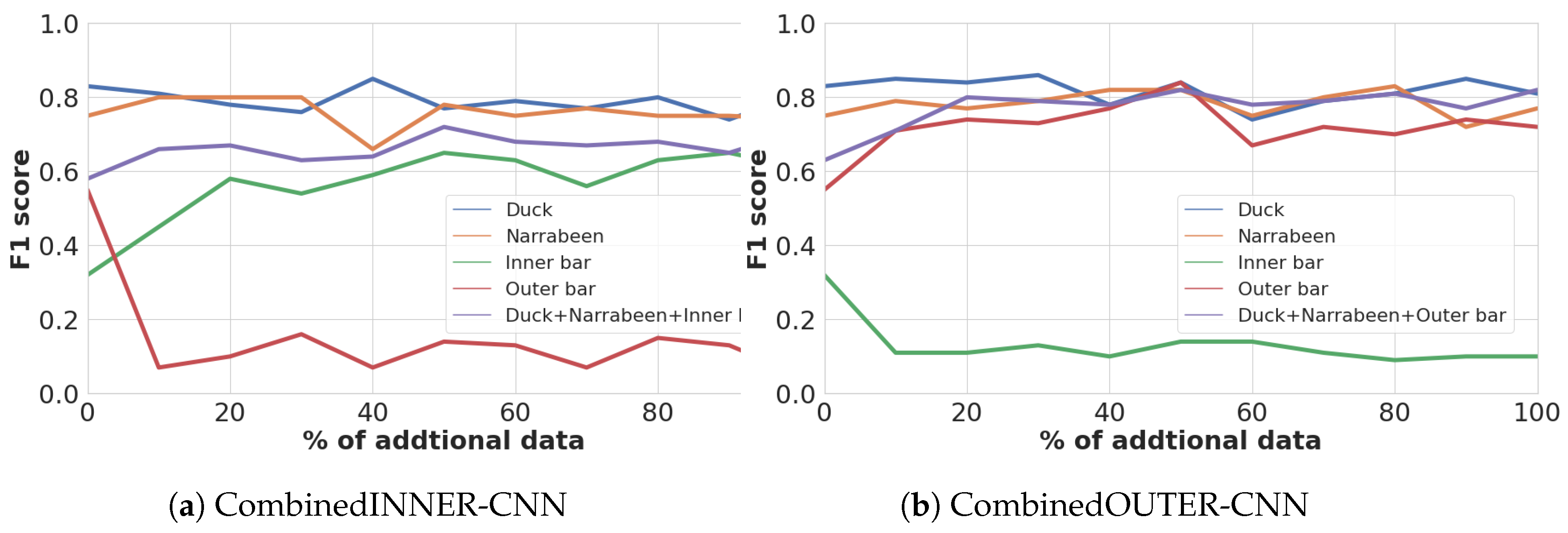
5.2. Double-Bar Beach Models Performances
6. Discussion
6.1. Single-Bar Models
6.2. Double-Bar Models
7. Conclusions
Author Contributions
Funding
Data Availability Statement
Acknowledgments
Conflicts of Interest
Appendix A. Performance in Terms of Loss
Appendix A.1. Single-Bar Models

Appendix A.2. Double-Bar Models


References
- Plant, N.; Holman, R.; Freilich, M.; Birkemeier, W. A simple model for interannual sandbar behavior. J. Geophys. Res. Ocean. 1999, 104, 15755–15776. [Google Scholar] [CrossRef]
- Walstra, D.J.R.; Wesselman, D.A.; Van der Deijl, E.C.; Ruessink, G. On the intersite variability in inter-annual nearshore sandbar cycles. J. Mar. Sci. Eng. 2016, 4, 15. [Google Scholar] [CrossRef]
- Alexander, P.S.; Holman, R.A. Quantification of nearshore morphology based on video imaging. Mar. Geol. 2004, 208, 101–111. [Google Scholar] [CrossRef]
- Holman, R.A.; Symonds, G.; Thornton, E.B.; Ranasinghe, R. Rip spacing and persistence on an embayed beach. J. Geophys. Res. Ocean. 2006, 111, C01006. [Google Scholar] [CrossRef]
- Tătui, F.; Constantin, S. Nearshore sandbars crest position dynamics analysed based on Earth Observation data. Remote Sens. Environ. 2020, 237, 111555. [Google Scholar] [CrossRef]
- Castelle, B.; Marieu, V.; Bujan, S.; Splinter, K.D.; Robinet, A.; Sénéchal, N.; Ferreira, S. Impact of the winter 2013–2014 series of severe Western Europe storms on a double-barred sandy coast: Beach and dune erosion and megacusp embayments. Geomorphology 2015, 238, 135–148. [Google Scholar] [CrossRef]
- Almar, R.; Castelle, B.; Ruessink, B.; Sénéchal, N.; Bonneton, P.; Marieu, V. Two-and three-dimensional double-sandbar system behaviour under intense wave forcing and a meso–macro tidal range. Cont. Shelf Res. 2010, 30, 781–792. [Google Scholar] [CrossRef]
- Grant, S.B.; Kim, J.H.; Jones, B.H.; Jenkins, S.A.; Wasyl, J.; Cudaback, C. Surf zone entrainment, along-shore transport, and human health implications of pollution from tidal outlets. J. Geophys. Res. Ocean. 2005, 110, C10025. [Google Scholar] [CrossRef]
- Castelle, B.; Scott, T.; Brander, R.; McCarroll, R. Rip current types, circulation and hazard. Earth-Sci. Rev. 2016, 163, 1–21. [Google Scholar] [CrossRef]
- Short, A.D.; Aagaard, T. Single and multi-bar beach change models. J. Coast. Res. 1993, 15, 141–157. [Google Scholar]
- Price, T.; Ruessink, B. State dynamics of a double sandbar system. Cont. Shelf Res. 2011, 31, 659–674. [Google Scholar] [CrossRef]
- Wright, L.D.; Short, A.D. Morphodynamic variability of surf zones and beaches: A synthesis. Mar. Geol. 1984, 56, 93–118. [Google Scholar] [CrossRef]
- Van Enckevort, I.; Ruessink, B.; Coco, G.; Suzuki, K.; Turner, I.; Plant, N.G.; Holman, R.A. Observations of nearshore crescentic sandbars. J. Geophys. Res. Ocean. 2004, 109, C06028. [Google Scholar] [CrossRef]
- Abessolo Ondoa, G. Response of Sandy Beaches in West Africa, Gulf of Guinea, to Multi-Scale Forcing. Ph.D. Thesis, Université Paul Sabatier—Toulouse III, Toulouse, France, 2020. [Google Scholar]
- Gallagher, E.L.; Elgar, S.; Guza, R.T. Observations of sand bar evolution on a natural beach. J. Geophys. Res. Ocean. 1998, 103, 3203–3215. [Google Scholar] [CrossRef]
- Holman, R.A.; Stanley, J. The history and technical capabilities of Argus. Coast. Eng. 2007, 54, 477–491. [Google Scholar] [CrossRef]
- Holman, R.; Haller, M.C. Remote sensing of the nearshore. Annu. Rev. Mar. Sci. 2013, 5, 95–113. [Google Scholar] [CrossRef]
- Aarninkhof, S.; Ruessink, G. Quantification of surf zone bathymetry from video observations of wave breaking. In Proceedings of the AGU Fall Meeting Abstracts, San Francisco, CA, USA, 6–10 December 2002; Volume 2002, p. OS52E-10. [Google Scholar]
- Aleman, N.; Certain, R.; Robin, N.; Barusseau, J.P. Morphodynamics of slightly oblique nearshore bars and their relationship with the cycle of net offshore migration. Mar. Geol. 2017, 392, 41–52. [Google Scholar] [CrossRef]
- Palmsten, M.L.; Brodie, K.L. The Coastal Imaging Research Network (CIRN). Remote Sens. 2022, 14, 453. [Google Scholar] [CrossRef]
- Jackson, D.W.; Short, A.D.; Loureiro, C.; Cooper, J.A.G. Beach morphodynamic classification using high-resolution nearshore bathymetry and process-based wave modelling. Estuar. Coast. Shelf Sci. 2022, 268, 107812. [Google Scholar] [CrossRef]
- Janowski, L.; Wroblewski, R.; Rucinska, M.; Kubowicz-Grajewska, A.; Tysiac, P. Automatic classification and mapping of the seabed using airborne LiDAR bathymetry. Eng. Geol. 2022, 301, 106615. [Google Scholar] [CrossRef]
- Pape, L.; Ruessink, B. Neural-network predictability experiments for nearshore sandbar migration. Cont. Shelf Res. 2011, 31, 1033–1042. [Google Scholar] [CrossRef]
- Kingston, K.; Ruessink, B.; Van Enckevort, I.; Davidson, M. Artificial neural network correction of remotely sensed sandbar location. Mar. Geol. 2000, 169, 137–160. [Google Scholar] [CrossRef]
- Pape, L.; Ruessink, B.G.; Wiering, M.A.; Turner, I.L. Recurrent neural network modeling of nearshore sandbar behavior. Neural Netw. 2007, 20, 509–518. [Google Scholar] [CrossRef]
- Collins, A.M.; Geheran, M.P.; Hesser, T.J.; Bak, A.S.; Brodie, K.L.; Farthing, M.W. Development of a Fully Convolutional Neural Network to Derive Surf-Zone Bathymetry from Close-Range Imagery of Waves in Duck, NC. Remote Sens. 2021, 13, 4907. [Google Scholar] [CrossRef]
- Alzubaidi, L.; Zhang, J.; Humaidi, A.J.; Al-Dujaili, A.; Duan, Y.; Al-Shamma, O.; Santamaría, J.; Fadhel, M.A.; Al-Amidie, M.; Farhan, L. Review of deep learning: Concepts, CNN architectures, challenges, applications, future directions. J. Big Data 2021, 8, 53. [Google Scholar] [CrossRef]
- Goodfellow, I.; Bengio, Y.; Courville, A. Deep Learning; MIT Press: Cambridge, MA, USA, 2016. [Google Scholar]
- Yu, J.; Wang, Z.; Vasudevan, V.; Yeung, L.; Seyedhosseini, M.; Wu, Y. Coca: Contrastive captioners are image-text foundation models. arXiv 2022, arXiv:2205.01917. [Google Scholar]
- Gu, J.; Wang, Z.; Kuen, J.; Ma, L.; Shahroudy, A.; Shuai, B.; Liu, T.; Wang, X.; Wang, G.; Cai, J.; et al. Recent advances in convolutional neural networks. Pattern Recognit. 2018, 77, 354–377. [Google Scholar] [CrossRef]
- Hoshen, Y.; Weiss, R.J.; Wilson, K.W. Speech acoustic modeling from raw multichannel waveforms. In Proceedings of the 2015 IEEE International Conference on Acoustics, Speech and Signal Processing (ICASSP), South Brisbane, Australia, 19–24 April 2015; IEEE: Piscataway, NJ, USA, 2015; pp. 4624–4628. [Google Scholar]
- Krizhevsky, A.; Sutskever, I.; Hinton, G.E. Imagenet classification with deep convolutional neural networks. Adv. Neural Inf. Process. Syst. 2012, 25, 1097–1105. [Google Scholar] [CrossRef]
- Parkhi, O.M.; Vedaldi, A.; Zisserman, A. Deep face recognition. arXiv 2015, arXiv:1804.06655. [Google Scholar]
- Niu, S.; Liu, Y.; Wang, J.; Song, H. A decade survey of transfer learning (2010–2020). IEEE Trans. Artif. Intell. 2020, 1, 151–166. [Google Scholar] [CrossRef]
- Castelluccio, M.; Poggi, G.; Sansone, C.; Verdoliva, L. Land use classification in remote sensing images by convolutional neural networks. arXiv 2015, arXiv:1508.00092. [Google Scholar]
- Ellenson, A.N.; Simmons, J.A.; Wilson, G.W.; Hesser, T.J.; Splinter, K.D. Beach State Recognition Using Argus Imagery and Convolutional Neural Networks. Remote Sens. 2020, 12, 3953. [Google Scholar] [CrossRef]
- Birkemeier, W.A.; DeWall, A.E.; Gorbics, C.S.; Miller, H.C. A User’s Guide to CERC’s Field Research Facility; Technical Report; Coastal Engineering Research Center: Fort Belvoir VA, USA, 1981. [Google Scholar]
- Lee, G.h.; Nicholls, R.J.; Birkemeier, W.A. Storm-driven variability of the beach-nearshore profile at Duck, North Carolina, USA, 1981–1991. Mar. Geol. 1998, 148, 163–177. [Google Scholar] [CrossRef]
- Stauble, D.K.; Cialone, M.A. Sediment dynamics and profile interactions: Duck94. In Proceedings of the Coastal Engineering 1996, Orlando, FL, USA, 2–6 September 1996; pp. 3921–3934. [Google Scholar]
- Turner, I.L.; Harley, M.D.; Short, A.D.; Simmons, J.A.; Bracs, M.A.; Phillips, M.S.; Splinter, K.D. A multi-decade dataset of monthly beach profile surveys and inshore wave forcing at Narrabeen, Australia. Sci. Data 2016, 3, 160024. [Google Scholar] [CrossRef]
- Splinter, K.D.; Harley, M.D.; Turner, I.L. Remote sensing is changing our view of the coast: Insights from 40 years of monitoring at Narrabeen-Collaroy, Australia. Remote Sens. 2018, 10, 1744. [Google Scholar] [CrossRef]
- Harley, M.D.; Turner, I.; Short, A.; Ranasinghe, R. A reevaluation of coastal embayment rotation: The dominance of cross-shore versus alongshore sediment transport processes, Collaroy-Narrabeen Beach, southeast Australia. J. Geophys. Res. Earth Surf. 2011, 116, F04033. [Google Scholar] [CrossRef]
- Harley, M. Coastal storm definition. In Coastal Storms: Processes and Impacts; Wiley–Blackwell: Hoboken, NJ, USA, 2017; pp. 1–21. [Google Scholar]
- Short, A.D.; Trenaman, N. Wave climate of the Sydney region, an energetic and highly variable ocean wave regime. Mar. Freshw. Res. 1992, 43, 765–791. [Google Scholar] [CrossRef]
- Strauss, D.; Mirferendesk, H.; Tomlinson, R. Comparison of two wave models for Gold Coast, Australia. J. Coast. Res. 2007, 50, 312–316. [Google Scholar]
- Allen, M.; Callaghan, J. Extreme Wave Conditions for the South Queensland Coastal Region; Environmental Protection Agency: Brisbane, Australia, 2000.
- Jackson, L.A.; Tomlinson, R.; Nature, P. 50 years of seawall and nourishment strategy evolution on the gold coast. In Proceedings of the Australasian Coasts & Ports conference, Cairns, Australia, 21–23 June 2017; pp. 640–645. [Google Scholar]
- Jackson, L.A.; Tomlinson, R.; Turner, I.; Corbett, B.; d’Agata, M.; McGrath, J. Narrowneck artificial reef; results of 4 yrs monitoring and modifications. In Proceedings of the 4th International Surfing Reef Symposium, Manhattan Beach, CA, USA, 12–14 January 2005. [Google Scholar]
- Turner, I.L.; Whyte, D.; Ruessink, B.; Ranasinghe, R. Observations of rip spacing, persistence and mobility at a long, straight coastline. Mar. Geol. 2007, 236, 209–221. [Google Scholar] [CrossRef]
- Khan, A.; Sohail, A.; Zahoora, U.; Qureshi, A.S. A survey of the recent architectures of deep convolutional neural networks. Artif. Intell. Rev. 2020, 53, 5455–5516. [Google Scholar] [CrossRef]
- Shrestha, A.; Mahmood, A. Review of deep learning algorithms and architectures. IEEE Access 2019, 7, 53040–53065. [Google Scholar] [CrossRef]
- Huang, G.; Liu, Z.; Van Der Maaten, L.; Weinberger, K.Q. Densely connected convolutional networks. In Proceedings of the IEEE Conference on Computer Vision and Pattern Recognition, Honolulu, HI, USA, 21–26 July 2017; pp. 4700–4708. [Google Scholar]
- Simonyan, K.; Zisserman, A. Very deep convolutional networks for large-scale image recognition. arXiv 2014, arXiv:1409.1556. [Google Scholar]
- Szegedy, C.; Vanhoucke, V.; Ioffe, S.; Shlens, J.; Wojna, Z. Rethinking the inception architecture for computer vision. In Proceedings of the IEEE Conference on Computer Vision and Pattern Recognition, Las Vegas, NV, USA, 27–30 June 2016; pp. 2818–2826. [Google Scholar]
- He, K.; Zhang, X.; Ren, S.; Sun, J. Deep residual learning for image recognition. In Proceedings of the IEEE Conference on Computer Vision and Pattern Recognition, Las Vegas, NV, USA, 27–30 June 2016; pp. 770–778. [Google Scholar]
- Yamashita, R.; Nishio, M.; Do, R.K.G.; Togashi, K. Convolutional neural networks: An overview and application in radiology. Insights Imaging 2018, 9, 611–629. [Google Scholar] [CrossRef] [PubMed]
- Russakovsky, O.; Deng, J.; Su, H.; Krause, J.; Satheesh, S.; Ma, S.; Huang, Z.; Karpathy, A.; Khosla, A.; Bernstein, M.; et al. Imagenet large scale visual recognition challenge. Int. J. Comput. Vis. 2015, 115, 211–252. [Google Scholar] [CrossRef]
- Pan, S.J.; Yang, Q. A survey on transfer learning. IEEE Trans. Knowl. Data Eng. 2009, 22, 1345–1359. [Google Scholar] [CrossRef]
- Tan, C.; Sun, F.; Kong, T.; Zhang, W.; Yang, C.; Liu, C. A survey on deep transfer learning. In Proceedings of the International Conference on Artificial Neural Networks, Rhodes, Greece, 4–7 October 2018; Springer: New York, NY, USA, 2018; pp. 270–279. [Google Scholar]
- Smith, L.N.; Topin, N. Super-convergence: Very fast training of neural networks using large learning rates. In Proceedings of the Artificial Intelligence and Machine Learning for Multi-Domain Operations Applications, Baltimore, MD, USA, 15–17 April 2019; International Society for Optics and Photonics: Bellingham, WA, USA, 2019; Volume 11006, p. 1100612. [Google Scholar]
- Zhang, T.; Yu, B. Boosting with early stopping: Convergence and consistency. Ann. Stat. 2005, 33, 1538–1579. [Google Scholar] [CrossRef]
- Yang, J.; Yang, G. Modified convolutional neural network based on dropout and the stochastic gradient descent optimizer. Algorithms 2018, 11, 28. [Google Scholar] [CrossRef]
- Menardi, G.; Torelli, N. Training and assessing classification rules with imbalanced data. Data Min. Knowl. Discov. 2014, 28, 92–122. [Google Scholar] [CrossRef]
- Cubuk, E.D.; Zoph, B.; Mane, D.; Vasudevan, V.; Le, Q.V. Autoaugment: Learning augmentation strategies from data. In Proceedings of the IEEE/CVF Conference on Computer Vision and Pattern Recognition, Long Beach, CA, USA, 15–19 June 2019; pp. 113–123. [Google Scholar]
- Hossin, M.; Sulaiman, M.N. A review on evaluation metrics for data classification evaluations. Int. J. Data Min. Knowl. Manag. Process 2015, 5, 1. [Google Scholar]
- Pianca, C.; Holman, R.; Siegle, E. Shoreline variability from days to decades: Results of long-term video imaging. J. Geophys. Res. Ocean. 2015, 120, 2159–2178. [Google Scholar] [CrossRef]
- Lei, S.; Zhang, H.; Wang, K.; Su, Z. How Training Data Affect the Accuracy and Robustness of Neural Networks for Image Classification. In Proceedings of the International Conference on Learning Representations (ICLR 2019), New Orleans, LA, USA, 6–9 May 2019. [Google Scholar]
- Jiang, B.; Luo, R.; Mao, J.; Xiao, T.; Jiang, Y. Acquisition of localization confidence for accurate object detection. In Proceedings of the European Conference on Computer Vision (ECCV), Munich, Germany, 8–14 September 2018; pp. 784–799. [Google Scholar]
- Bashir, F.; Porikli, F. Performance evaluation of object detection and tracking systems. In Proceedings of the 9th IEEE International Workshop on PETS, New York, NY, USA, 18 June 2006; pp. 7–14. [Google Scholar]


| State | Duck | Narrabeen (*) | Gold Coast Inner Bar | Gold Coast Outer Bar |
|---|---|---|---|---|
| R | 125 | 125 (0) | 377 | 0 |
| LTT | 126 | 164 (+7) | 1779 | 0 |
| TBR | 140 | 157 (+8) | 596 | 1118 |
| RBB | 126 | 106 (−24) | 74 | 746 |
| LBT | 163 | 135 (+9) | 197 | 1159 |
| Total | 680 | 687 | 3023 | 3023 |
| Type | Parameter | Setting |
|---|---|---|
| OneCycleLR | Max momentum | 0.95 |
| OneCycleLR | Min momentum | 0.85 |
| OneCycleLR | Max learning rate | 0.01 |
| SGD | Learning rate | 0.002 |
| Network | Batch size | 32 |
| Early stopping | Patience | 20 |
| Augmentation | Function |
|---|---|
| RandomRotation (15) | Rotate the image randomly between 0 and 15 degree angles |
| AutoAugment | Data augmentation method based on the proposed method of [64]. |
| RandomAffine (0, translate = (0.15, 0.20)) | Random affine transformation (translation with horizontal translates randomly between maximum fractions of 15 and 20) of the image, keeping the center invariant. |
| Experiment | Model Name | Training Data |
|---|---|---|
| 1. | DUCK-CNN | Duck |
| NBN-CNN | Narrabeen | |
| CombinedSINGLE-CNN | Duck & Narrabeen | |
| 2. | INNER-CNN | Gold Coast’s inner bar labels |
| OUTER-CNN | Gold Coast’s outer bar labels | |
| CombinedINNER-CNN | Duck, Narrabeen & Gold Coast’s inner bar labels | |
| CombinedOUTER-CNN | Duck, Narrabeen & Gold Coast’s outer bar labels |
| Experiment | Model Name | Test Data | ||||
|---|---|---|---|---|---|---|
| Self-Tests | Transfer-Tests | |||||
| 1. | DUCK-CNN | Duck | Narrabeen | |||
| NBN-CNN | Narrabeen | Duck | ||||
| CombinedSINGLE-CNN | Duck & Narrabeen | Duck | Narrabeen | Gold Coast | ||
| 2. | INNER-CNN | Gold Coast’s inner bar labels | - | |||
| OUTER-CNN | Gold Coast’s outer bar labels | - | ||||
| CombinedINNER-CNN | Duck, Narrabeen & Gold Coast | Duck | Narrabeen | Gold Coast | - | |
| CombinedOUTER-CNN | Duck, Narrabeen & Gold Coast | Duck | Narrabeen | Gold Coast | - | |
| Classified | |||
|---|---|---|---|
| Actual | Yes | No | |
| Yes | |||
| No | |||
| F1 Values | ||
|---|---|---|
| Model | Duck | Narrabeen |
| NBN-CNN | 0.66 | 0.76 |
| DUCK-CNN | 0.89 | 0.73 |
| CombinedSINGLE-CNN | 0.85 | 0.78 |
| 0.78 | ||
Publisher’s Note: MDPI stays neutral with regard to jurisdictional claims in published maps and institutional affiliations. |
© 2022 by the authors. Licensee MDPI, Basel, Switzerland. This article is an open access article distributed under the terms and conditions of the Creative Commons Attribution (CC BY) license (https://creativecommons.org/licenses/by/4.0/).
Share and Cite
Oerlemans, S.C.M.; Nijland, W.; Ellenson, A.N.; Price, T.D. Image-Based Classification of Double-Barred Beach States Using a Convolutional Neural Network and Transfer Learning. Remote Sens. 2022, 14, 4686. https://doi.org/10.3390/rs14194686
Oerlemans SCM, Nijland W, Ellenson AN, Price TD. Image-Based Classification of Double-Barred Beach States Using a Convolutional Neural Network and Transfer Learning. Remote Sensing. 2022; 14(19):4686. https://doi.org/10.3390/rs14194686
Chicago/Turabian StyleOerlemans, Stan C. M., Wiebe Nijland, Ashley N. Ellenson, and Timothy D. Price. 2022. "Image-Based Classification of Double-Barred Beach States Using a Convolutional Neural Network and Transfer Learning" Remote Sensing 14, no. 19: 4686. https://doi.org/10.3390/rs14194686
APA StyleOerlemans, S. C. M., Nijland, W., Ellenson, A. N., & Price, T. D. (2022). Image-Based Classification of Double-Barred Beach States Using a Convolutional Neural Network and Transfer Learning. Remote Sensing, 14(19), 4686. https://doi.org/10.3390/rs14194686