Article

An Efficient Information-Reinforced Lidar Deep Completion Network without RGB Guided

1
Changchun Institute of Optics, Fine Mechanics and Physics, Chinese Academy of Sciences, Changchun 130033, China
2
University of Chinese Academy of Sciences, Beijing 100049, China
*
Author to whom correspondence should be addressed.
Remote Sens. 2022, 14(19), 4689; https://doi.org/10.3390/rs14194689
Submission received: 24 August 2022 / Revised: 13 September 2022 / Accepted: 18 September 2022 / Published: 20 September 2022

Abstract

:
Due to the sparsity of point clouds obtained by LIDAR, the depth information is usually not complete and dense. The depth completion task is to recover dense depth information from sparse depth information. However, most of the current deep completion networks use RGB images as guidance, which are more like a processing method of information fusion. They are not valid when there is only sparse depth data and no other color information. Therefore, this paper proposes an information-reinforced completion network for a single sparse depth input. We use a multi-resolution dense progressive fusion structure to maximize the multi-scale information and optimize the global situation by point folding. At the same time, we re-aggregate the confidence and impose another depth constraint on the pixel depth to make the depth estimation closer to the ground trues. Our experimental results on KITTI and NYU Depth v2 datasets show that the proposed network achieves better results than other unguided deep completion methods. And it is excellent in both accuracy and real-time performance.

Graphical Abstract

1. Introduction

With the gradual expansion of computer vision applications, all walks of life have higher requirements for depth information. Accurate depth data is essential for self-driving cars, autonomous navigation systems, and virtual reality [1]. However, depth is often sparse and partially missing due to device and environmental limitations. It is fatal in the reconstruction of 3D information [2]. Therefore, the completion methods of the sparse depth data have been widely studied in recent years [3,4]. However, traditional methods often fail to achieve good results because of the sparsity and lack of sufficient prior knowledge of the missing depth [5,6]. With the development of deep learning, people began to use deep neural networks to complete the depth information and achieve better results than the traditional interpolation methods [7,8].
At present, most depth completion networks supplement the missing depth information through the guidance of RGB images [9]. It can provide effective real edges to distinguish the contours between objects. The mapping relationship between sparse depth and a color image is established image through network learning [10,11]. And then the dense depth is regressed together [12]. Although they achieve a better result, these data are based on the joint action of multiple sensors, which requires the important premise that the image and the point cloud correspond to each other. The problem can be effectively controlled in the datasets. However, the joint calibration of heterogeneous sensors will increase the cost and uncertain error, and the reliability of the function cannot be guaranteed in practical application [13,14]. Therefore, our network no longer uses any RGB image to guide and only relies on a single sparse depth image to complete the depth to be more suitable for real-world scenarios. We use the confidence re-aggregation to consider the depth reliability of the neighborhood and obtain the most accurate local pixel depth estimation. In fact, the depth of the outdoors is more complex and variable than the interior. The overall texture is required to be enhanced, and the range of variation of each target is required to be enlarged. Therefore, we further research the information processing of autonomous driving. We design the structural multi-resolution dense progressive fusion processing and point folding module to further improve the accuracy of global prediction in autonomous driving. We cancel the additional information of RGB images and use only one-fourth of the information of other methods [15,16], which avoids the necessary complex and error operations such as joint calibration and calibration in actual use. It greatly reduces the volume of the network and achieves the requirements of accuracy and speed, which is more suitable for the real-world situation.
In fact, it is difficult to achieve good results by only entering depth information because of the limitation of information content [17,18]. Researchers have come up with several ideas for solving. SI-Net [19] found that ordinary convolution directly used to complete depth could not achieve good results. They proposed a simple and effective sparse convolution layer, which weighted the elements of the convolution kernel according to the validity of the input pixels. Then they transferred the information about the validity of pixels to the subsequent layers of the network. The improvement makes the deep completion task based on a convolutional neural network successful. The relationship between convolution and confidence has become a research hotspot in this field [20,21]. Considering that the use of confidence as a binary value mask to filter out lost measurements can ignore valuable information in the confidence map, N-CNN [22] proposed an algebraic constrained convolutional layer for sparse input CNNS. They used signal confidence as a continuous measure of data uncertainty and convolution constrained by confidence to achieve superior performance. However, Spade [8] believed that sparse convolution is not necessary. They used the ordinary dense CNN architecture and the new sparse training strategy to produce significantly better performance. However, it depends on the change of training mode, and the robustness is poor. According to HMS-NET [23], sparse invariant convolution not only loses numerous spatial information but also cannot be directly integrated into multi-scale structures. Therefore, they proposed three sparse invariant operations for processing sparse inputs and feature maps. And they designed a hierarchical multi-scale network structure that integrates information of different scales to solve the deep completion task.
SPN [24] combined global and local information to learn confidence in an unsupervised manner. The predicted depth maps are weighted by the respective confidence maps. On this basis, PNCNN [25] learned the input confidence estimator in a self-supervised way based on a normalized convolutional neural network to identify the interference measurements in the input. They proposed a probabilistic version of NCNN that produces a statistically meaningful measure of uncertainty for the final prediction. However, the reliability of the effect cannot be guaranteed when the completion result is directly used for the subsequent judgment of depth because the confidence degree is not supervised by the truth value in the learning of these networks. As sparse information provided by spare depth is limited, we should make full use of the local neighborhood information to strengthen the dependence relationship of the neighborhood [26,27].
An affinity is a display form of neighborhood information, which can represent the coherence of color and texture and the similarity between pixels and pixels at the semantic level. But it is not usually seen as part of the learning problem [28]. SPN [24] proposed spatial propagation networks that use learned affinities to guide and disseminate information in images. All modules are differentiable and jointly trained using stochastic gradient descent methods, which are also computationally very efficient. Based on this, CSPN [29] proposed a convolution space propagation network. It no longer scans row/column propagation from four directions like SPN [24] but propagates in parallel through recursive convolution operation. Learning the affinity between adjacent pixels by the deep convolutional neural network can improve the effectiveness and speed of the deep completion task. However, the mode of propagation has a definite limitation, requiring a fixed local neighborhood configuration for propagation. Once the local neighbor is fixed, there will be irrelevant information mixed with the reference information, resulting in the mixing depth problem, especially at the depth boundary. Therefore, NLSPN [30] introduced a learnable affinity normalization method to learn affinity combinations better. They avoided the irrelevant local neighborhood effectively and focused on the relevant non-local neighborhood in the propagation process. However, it has a strong dependence on the neighborhood and a low dependence on confidence. In addition, it takes numerous iterations to receive good results. The complex calculation makes the speed decrease greatly and cannot meet the real-time demand. Based on CSPN [29], DSPN [31] decoupled the neighborhood into different parts according to different distances, generates independent attention graphs recursively, and refines these parts into adaptive affinity matrices. However, it is still based on sparse depth and color image fusion. Therefore, we put forward the idea of confidence reaggregation. We learn neighborhood affinity in the form of spatial propagation and further refine local depth in order to improve the accuracy of depth completion.
In addition, global information is crucial to the complete effect. The multi-scale structure can enhance the reliability of global information, which is very useful for sparse depth of missing information [32]. U-Net [33] designed the contraction path and expansion path following the typical architecture of convolutional networks, and effectively become the main framework for various other tasks to solve the problem of medical image segmentation. Most networks added different residual structures to the U-Net [33] framework with improved points to learn features with different resolutions, which solves the degradation problem and greatly improves the fitting ability of neural networks. However, it only makes up for the loss of resolution caused by convolution and ignores the original information of different resolutions. Therefore, we design a dense progressive fusion multi-scale structure as a complement to the global information to make maximum use of the existing original information. The global completion effect is improved by fusing the global depth information of different scales.
Depth completion is essentially the same as point cloud completion. They are both estimates of 3D information. The difference lies in the way they represent three-dimensional information. Folding-Net [34] wrapped a constant 2D grid into the shape of an input 3D point cloud in the point cloud completion task. Since the network integrates mappings from lower dimensions, it increases the possibility of more points. Similarly, for sparse depth images, the possibility of more pixels requests to be added. Therefore, we designed a point folding module from 1D to 2D to integrate the one-dimensional point information into the missing two-dimensional information through the learning of the network to strengthen the density of the overall depth. It can increase the density of global information.
In summary, we construct a deep completion network with a single sparse depth input that integrates local and global information, which strengthens the known information and does not require any color image guidance (EIR-NET). Compared with other networks, the paper has the following contributions:
  • We propose a confidence re-aggregation method, which is re-aggregate the local area, effectively based on the confidence of the local pixel neighborhood to improve the estimation accuracy of local details.
  • We designed a dense progressive fusion network structure to further improve the accuracy of global completion by using multi-scale information.
  • We propose a 1D to 2D point folding module to increase the density of global depth information.

2. Methods

Our network structure is shown in Figure 1. The sparse depth image is input into the U-shaped network to obtain the initial confidence. The confidence is re-aggregated and optimized by the neighborhood information to obtain deep confidence in the confidence re-aggregation module. The confidence and original sparsity depth are input into the encoding of dense progressive fusion. The convolution results are fused layer by layer from different levels, and the different resolution information of multiple branches is used to supplement the details. We use the point folding module to increase the possibility of points and add it to the final fused feature code in the decoding. After that, the complete depth image is output as the final result.

2.1. Confidence Re-Aggregation Module

We can use convolution to extract features to obtain the confident prediction of depth images. However, there is no real supervision in the network learning, which makes the transmission volatility large. The resulting confidence prediction will have errors. As mentioned in the NLSPN [30], affinity normalization ensures stability and neighborhood correlation during propagation. We used absolute and normalized affinities (AS), regular absolute and normalized affinities (AS*), and hyperbolic tangent functions (TC) to experiment.
AS is restricted to the lines satisfying ω 1 + ω 2 = 1 after normalized affinity. It can be expressed as
A S ( ω m , n i , j ) = ω ^ m , n i , j / ( i , j ) N m , n | ω ^ m , n i , j |
where ω ^ represents the original confidence before normalization and ω represents the refined confidence after normalization. m and n represent the size of the window. i and j represent the coordinates.
AS* is restricted by
d ω d > 1
where d represents the different dimensions.
TC can be represented as
ω d = t a n h ( ω ^ d ) / C
where C represents the normalization factors. t a n h are hyperbolic tangent functions.
The essence of spatial a propagation network is to learn a large affinity matrix and transform its diffusion into local linear spatial propagation. It simply and effectively enhances the output. Similarly, we can use it to further enhance unreliable self-monitoring results. The difference is that our specification body is the confidence rather than the convolution. We describe the difference between confidence re-aggregation and normal confidence in Figure 2. The initial confidence is derived from the feature. According to the feature image, the affinity optimization of the initial confidence is carried out to obtain the fine confidence. Then the better feature images are obtained according to the fine confidence and initial feature images. As shown in Figure 1, the module is attached after the feature extraction to generate effective confidence in Step 1. After experiments, we chose absolute and normalized affinities (AS) as the aggregation method in Section 3.3.1.
Finally, we fuse the aggregate result with the original output and receive the new output to avoid degradation. The results of (a) and (b) in Figure 2 are fused on the channel, which can be expressed as
ω m , n i , j Φ B , C 1 + C 2 , H , W = c a t ( A S ( ω m , n i , j ) Φ B , C 1 , H , W , ω ^ m , n i , j Φ B , C 2 , H , W )
where Φ represents the representation of dimensions and size. B represents the batchsizes. C represents the channel, H and W represent the height and the weight. The structure of connections increases reliability and makes up for the defects caused by self-supervision.

2.2. Densely Progressive Fusion Module

We request to make the most of the depth map information because our network is not guided by color images. The loss of global information may directly lead to the omission of information. The image pyramid structure will receive different resolutions of depth and receive different scales of information. Making full use of the multi-resolution multi-branch structure can benefit the overall and detailed regression. Therefore, we design a new contraction path based on U-Net [33]. A U-shaped encoder architecture that follows the basic framework of convolution is generated, which is no longer completely symmetric with the expansion path of the decoder.
NCNN [22] is an effective way to fuse confidence and depth features. Similar to the operation of ordinary convolution, the normalized convolution is an operation in the domain of each point pair of the signal. The convolution at each point results in an effective inner product between the kernel of the conjugate and reflection filters and the neighborhood. For a sparse signal s , the finite neighborhood of each of its signals is defined in a finite space n C n . The confidence c R n of s represents the reliability of the neighborhood, which is usually nonnegative.
The local modeling approach of the signal is to project each sample onto a subspace spanned by basic functions. The signal s can be denoted as
S = B r
where B is a m × n matrix and r is the coordinates of the sample and the basic function concerning B . Thus, the least squares estimation of coordinates with weight matrix w can be obtained as
arg min r C n B r s w
Taking an applicability function a C n as the weight of the basis and a window function as the benchmark, we can receive the following solution:
r ^ = ( B * W B ) 1 B * W s = ( B * D a D c B ) 1 B * D a D c s
where the weight matrix W is the product of D a = D i a g ( a ) and D c = D i a g ( c ) . D i a g is the diagonal matrix. The equivalent inner product is expressed as follows:
r = ( b 1 , b 1 ) w ( b 1 , b m ) w ( b m , b 1 ) w ( b m , b m ) w 1 ( b 1 , f ) w ( b m , f ) w = ( a · c · b 1 , b 1 ) ( a · c · b 1 , b m ) ( a · c · b m , b 1 ) ( a · c · b m , b m ) 1 ( a · c · b 1 , f ) ( a · c · b m , f )
when choosing a constant function as the basis, we set B = 1 and can obtain:
r ^ = ( 1 * D a D c 1 ) 1 1 * D a D c s = a · ( c s ) a · c
where is the Hadamard product. Through convolution operation of signal s, we can obtain:
r ^ [ k ] = i n a [ i ] s [ k i ] c [ k i ] i n a [ i ] c [ k i ]
where k and i are the current coordinate and the unit coordinate in the formula for convolution in the discrete domain. n is the degree. The propagation value between normalized convolutional layers is:
c ^ i = a | c 1 n | a
where c i represents the confidence value of the i pixel. Although it is obtained by convolution calculation, the relationship between Windows is not tight enough. It hurts spatial transmission.
Aggregation can calculate the neighborhood correlation more accurately and enhance the local effect. The aggregated values are stored in the original space S , still in one-to-one correspondence with element positions. The energy function can be expressed as
x ( c ) = x o r i g i n a l ( c ) + x n e i g h b o r ( c ) = ω
where x o r i g i n a l and x n e i g h b o r are the original item and the neighborhood aggregation item, respectively.
PNCNN [25] proposed a probabilistic version of a normalized convolutional neural network by deriving the connection between normalized convolutional and statistical least squares methods. Define the signal s = B r + e , where e is a random noise variable with mean 0 and variance σ 2 V , then σ 2 is the global signal and V is a positive definite matrix describing the covariance between observations. It can be expressed as
W = V 1
The uncertain value is:
cov ( s ^ ) = cov ( B r ^ ) = B cov ( r ^ ) B *
After substituting in the calculation, it can be expressed as
cov ( s ^ ) = B ( ( B * V 1 B ) 1 B * V 1 s ) B * = σ 2 B ( B * V 1 B ) 1 B * = σ 2 B ( B * W a W c B ) 1 B *
when B = 1 , we can obtain:
c ^ = σ 2 1 ( 1 * W a W c 1 ) 1 1 * = σ 2 a | c
where the variance σ 2 has to be estimated. a and c are the applicability and output confidence of the last layer of the normalized convolutional neural network.
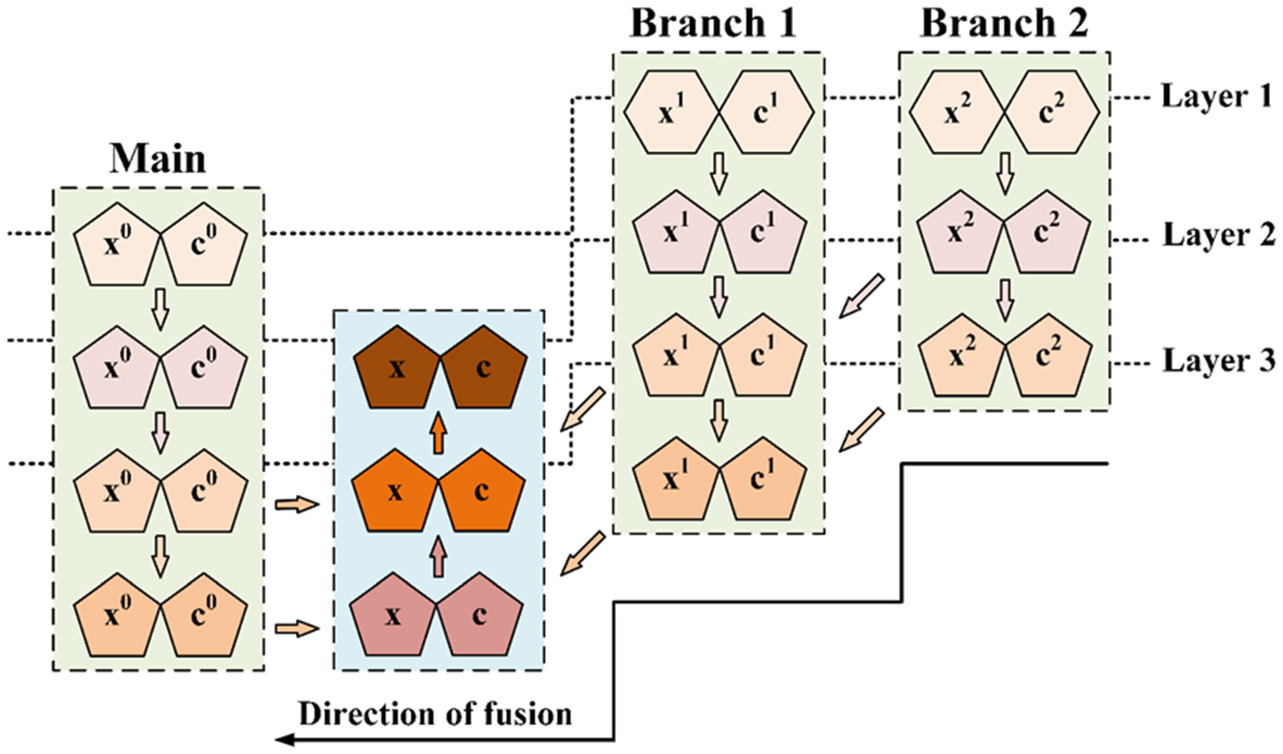
As shown in Figure 3, our dense progressive fusion structure is characterized by multi-branching and multi-resolution scales. The contraction path divides into three branches. The expansion path is a gradual step shape continuous fusion. It is more flexible and maneuverable than the ordinary U-shaped structure. We encode features through this hierarchical fusion structure in step 2, which is shown in Figure 1.
The corresponding confidence of the output features of different depths x ^ m , n i can be expressed as
c ^ m , n i = σ 2 a | c m , n 1 i
where i indicates the branch number. m represents the resolution scale. n represents the number of layers. Half of them are up-sampled and half of them are down-sampled. The transition sampling between m and m is defined as the 2-fold relation. x m , 0 i represents the original layer. i 0 , , i max 1 where i max = 3 . m 0 , , m max / 2 where m max = 8 .
Therefore, the results of the layer n in the down-sampling stage can be expressed as
x m , n i , c m , n i = n c o n v ( x m 1 , n 1 i , c m 1 , n 1 i )
The results of the layer n in the down-sampling stage can be obtained by progressive fusion of the main path and branch path and can be expressed as
x ^ m , n , c ^ m , n = c a t ( R m a i n , R b r a n c h ) = c a t ( n c o n v ( x m + 1 , n + 1 0 , c m + 1 , n + 1 0 ) , u p ( n c o n v ( x m 1 , n 1 0 , c m 1 , n 1 0 ) ) , u p ( n c o n v ( x m 1 , n 1 , c m 1 , n 1 ) ) , u p ( n c o n v ( x m 1 , n 1 2 , c m 1 , n 1 2 ) ) )

2.3. Point Folding Module

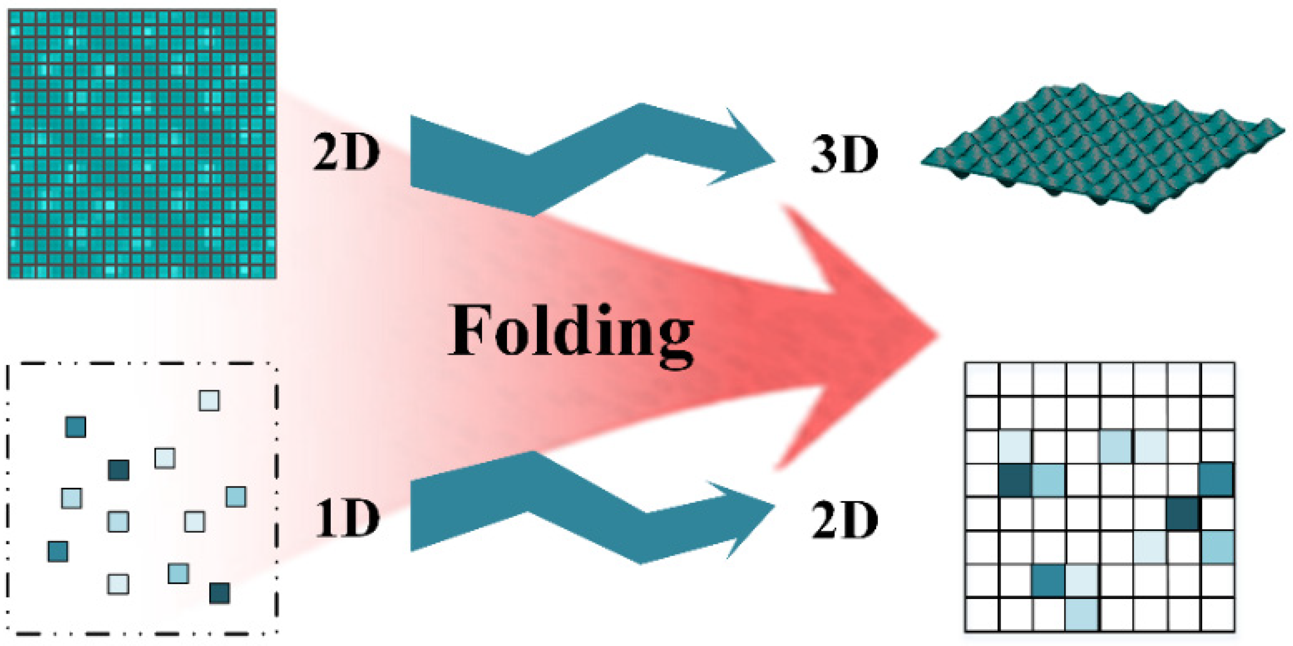
Folding-Net [34] complements spare depth by expanding 2D points into 3D point clouds through folding. The folding operation of reconstructed surfaces from 2D meshes fundamentally establishes the mapping from 2D regular fields to 3D point clouds. It acts as a filling and completion. Similarly, we can consider reducing the dimensionality to complement the 2D pixels with the 1D points. As shown in Figure 4, we expand the dimension of the folded network and use similar ideas to learn the completion depth information. As shown in Figure 1, we arranged it at the front of the decoder to enrich the encoded content and increase plasticity in Step 3. We fold 1D random points into the 2D grid.
The depth image D with size i × j and n random points folded can be expressed as
D = D ^ , { P | P i , j } = D ^ , { P | T r a n s ( p s ) }
where p s is the random point, s = 1 , , n . P i , j is the pixel folded into the grid. D ^ is the original depth image.

3. Experimental Evaluation

3.1. Datasets and Setup

KITTI-Depth [35]: The KITTI dataset is an authoritative and widely used deep completion dataset in vehicles. The author collected six hours of real traffic conditions. The dataset consists of calibrated and synchronized images, radar scans, high-precision GPS information, IMU acceleration information, and other modal information. Sparse depth images of the KITTI dataset were obtained by projecting the original LIDAR points onto the camera view. Ground truth semi-dense depth images are generated by projecting cumulative LIDAR scans of multiple time stamps and then removing abnormal depth values from occluded and moving objects. Since there are few LIDAR points at the top of the depth map, the bottom center of the input image is cropped. The remaining depth image has a resolution of 1256 × 352. In the depth completion dataset, a sparse depth image has about 6% valid pixels, while a ground truth depth image has about 14% valid pixels. The dataset contains 86,898 frames for training, 7000 frames for validating, and 1000 frames for testing.
NYU Depth v2 [36]: The NYU dataset is a color and depth camera from Microsoft Kinect, which consists of video sequences of various indoor scenes. According to the official method, we used about 50K images for training and 654 images for testing. We evaluated the effective region of 304 × 228 in order to match the resolution of RGB images and depth maps and compare it with other methods.
Our network runs on the Pytorch framework and is trained end-to-end on a single-stage NVIDIA GTX 2080 Ti GPU. During training, we use the Adam optimizer with β 1 = 0.9 , β 2 = 0.99 . The initial learning rate is 0.01 and decay of 10 1 every 3 epochs. We refer to the network parameters and the evaluation indicators of PNCNN [25] to compare the results fairly. We use the following common evaluation indicators to test our network performance. MAE is Mean Absolute Error (L1 loss). It is the mean of the distance between the model’s predicted value and the true value. Its convergence is fast and its gradient is stable. Therefore, it has a relatively robust solution. MSE is Mean Square Error (L2 Loss), which refers to the Mean squared difference between the predicted value of the model and the real sample value. Because its penalty is squared, it is sensitive to outliers. ABSREL is the Absolute Relative Error. RMSE stands for Root Mean Square Error. IMAE is Inverse Mean Absolute Error. IRMSE is Inverse Root Mean Square Error. DELTA is the percentage of pixels that are satisfied. MAE is shown in Equation (19). Other formulas can be expressed as
M S E = 1 n p P v n D p g t D p 2
A B S E R L = 1 n p P v n D p g t D p D p g t
R M S E = 1 n p P v n D p g t D p 2
I M A E = 1 n p P v n 1 D p g t 1 D p
I R M S E = 1 n p P v n 1 D p g t 1 D p 2
D E L T A τ = δ τ : max ( D p D p g t D p g t D p ) < τ , τ 1.25 , 1.25 2 , 1.25 3
where P v represents the set of valid pixels. D p g t represents the true value of the pixel p . D p represents the predicted value of the pixel p , and n represents the number of points.
Although the improvement of the loss function has achieved good results, the improvement effect is relatively small. Moreover, the improvement of the loss function of each network is targeted. It is poor in its extensiveness. While with L2 loss there are more outliers in the data, L2 will bring more errors due to the square operation. Therefore, L1 performs slightly better than L2 [8] in depth prediction. Therefore, we chose the most commonly used mean absolute error MAE (L1 loss) as the loss function of our network, which represents the sum of all absolute differences between the true and predicted values.

3.2. Results of Comparative Experiments

The completed results are shown in Figure 5. As shown in the figure, our network can effectively recover the depth of information and strengthen the density and integrity of 3D information. In some detail, the results are visually clear and obvious. Targets are clearly defined and easier to distinguish. It is very important for the further processing of 3D information.
Our results on KITTI are shown in Table 1, where our network (EIR-Net) achieves the best results with MAE and IMAE compared to other networks with a single depth input. The speed is similar to PNCNN, but all the indicators are better. Compared to the first two network models, our network speed is twice as slow, but the indicators are better than theirs. Compared to S2D++, both RMSE and IRMSE are worse. However, the difference is not much, only increased by 11.25% and 17.45%, but decreased by 27.89% and 32.35% in MAE and IMAE, respectively.
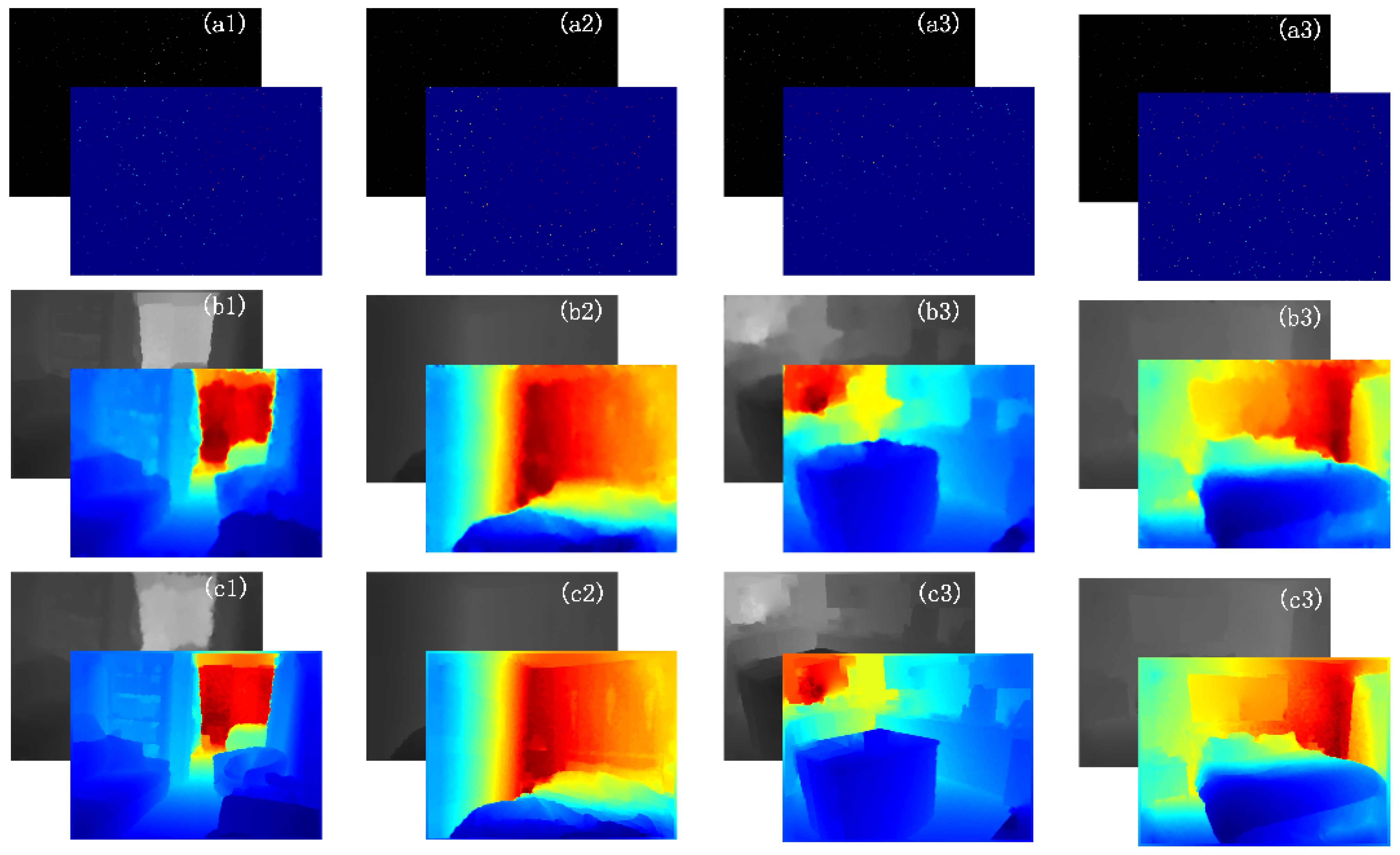
The completed results are shown in Figure 6. The depth of objects in the interior scene is effectively completed. Our results are shown in Table 2. Our network (EIR-Net) achieves the best results compared to other networks with a single deep input and some GRB-guided networks.

3.3. Results of the Ablation Experiments

3.3.1. Confidence Re-Aggregation Module

We used different methods to experiment. As can be seen from Table 3, re-aggregation is effective and the different aggregation methods have little impact on the loss function. At the same time, we found that the aggregation effect of AS is better than TC and AS*, and all indicators have been improved to different degrees. Finally, MAE decreased by 0.769, RMSE decreased by 1.611, IMAE decreased by 0.05, and IRMSE decreased by 8.058. In addition, these three methods take the same amount of time because the computation cost is the same. However, the time is only increased by 0.003 s to achieve the effect improvement. This means that the real-time performance of the network can still be guaranteed.
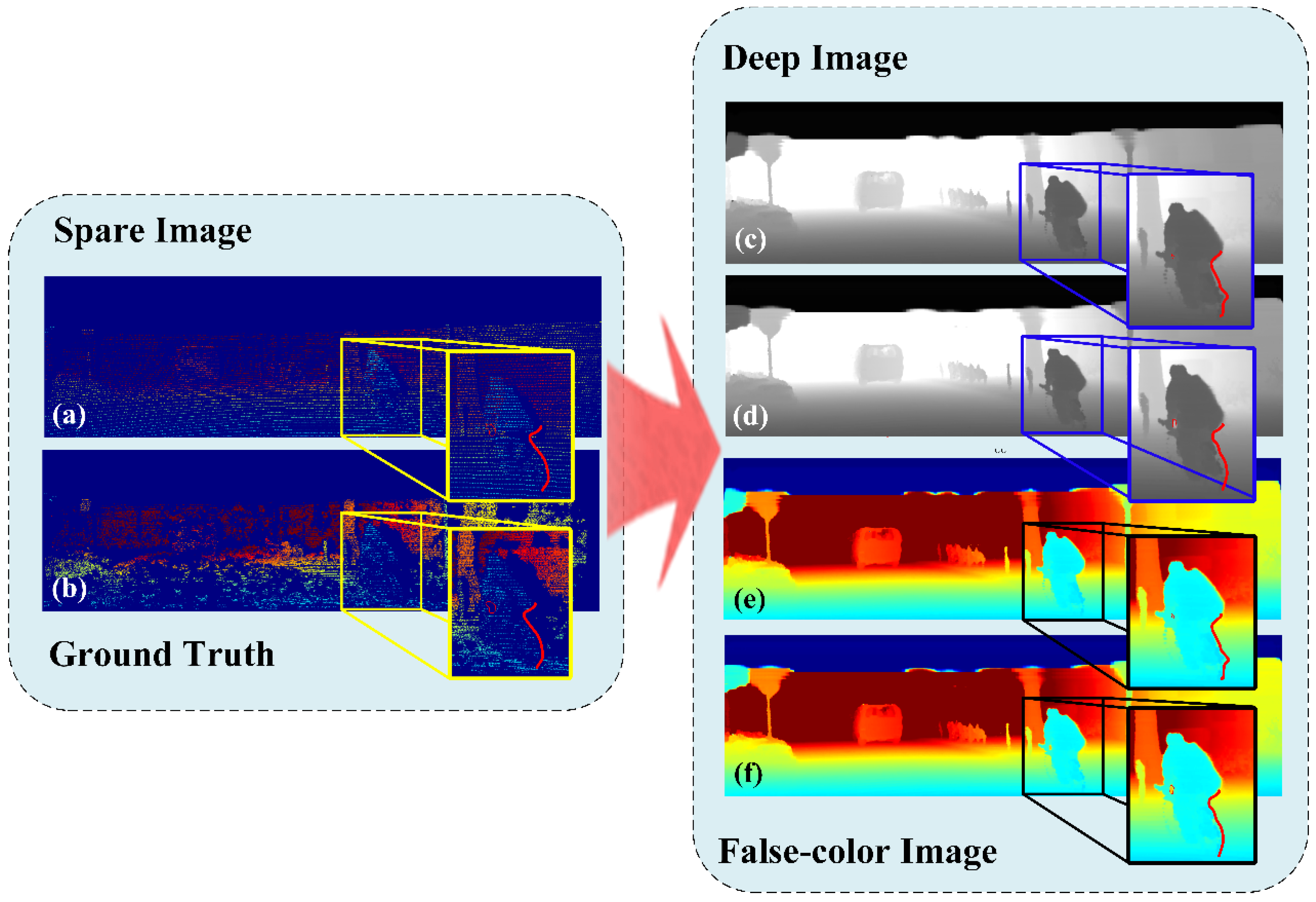
A more intuitive comparison is shown in Figure 7. We can find that the details are strengthened in the completed image after adding this module. Barely visible gaps are more fully displayed. In addition, the line of the back is smoother. Overall, we re-aggregated the confidence to strengthen the local detail effect, so that the outline of the person and the bicycle component is clearer.

3.3.2. Densely Progressive Fusion Module

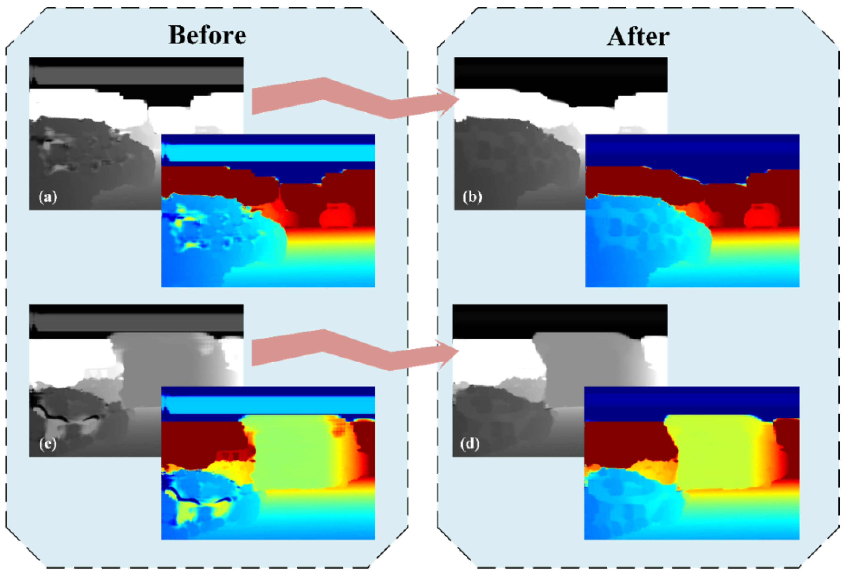
The effect of our dense progressive fusion Module is shown in Figure 8. From the previous frame, we can know that there is a car in the part marked in the box. However, the network lost the car in learning. The U-shaped structure of the network degrades the resolution in the network without intensive progressive fusion. The original information that can be learned is destroyed. The ideal situation of this position is a plane, and the blank space is output. However, after adding the dense progressive fusion module, we no longer learn features around a single branch but multiple branches in parallel. The combination of multi-resolution images and progressive fusion makes the network not lose any effective information globally. We show exactly where the car is in the image.
We find that the module can be used to compensate for the loss of detail due to the resolution gap. Most current network architectures use convolutional structures with varying resolutions. Therefore, a loss between resolutions can be caused by down-sampling. The module can not only be used in depth completion to fine details but also can be used in other fields to avoid local weakening.
The effect of our intensive progressive fusion is shown in Table 4. DPF represents dense progressive fusion module. (.) represents the number of layers. P-Folding represents the point folding module. Experiments show that the effect is improved. However, increasing the number of layers increases the time cost. In addition, the size of the resolution down-sampling is limited, and the number of layers is limited by the original size. Considering the real-time performance and the complexity of the structure, we choose two layers of DPF to add to our network to improve the global depth. Compared with the network without this module, MAE decreases by 0.776, RMSE decreases by 0.269, and IRMSE decreases by 0.4. IMAE increases, but only by 0.1. The pixel percentage of the second gradient increased by 0.001.

3.3.3. Point Folding Module

We show the point folding module in action in Figure 9. In the beginning, the car surface in the lower left corner does not have a good effect when the output completes the depth because the input depth is too sparse. The surface of the car is very uneven and large areas are missing. The point folding module can effectively supplement the missing part. As we can see, the surface depth of the car becomes flatter and denser with the addition of the point folding module. Further thinking, the shape of the car is more complete and clearer, which will be very conducive to improving the accuracy of 3D target recognition.
We show the effect of our dot fold module in the last row of Table 4. As we can see, the results are significantly improved compared to networks without this module. MAE decreased by 0.168, RMSE decreased by 1.879, IMAE decreased by 0.05, and IRMSE decreased by 1.989. The pixel percentages of the first and third gradients were increased by 0.005 and 0.001, respectively. There is no doubt that our module plays a role in optimizing the overall situation. The results of experiments show that our modules are efficient and portable not only when used separately but also when used in combination. The best results were obtained when we combine them.

4. Conclusions

In this paper, we designed a deep learning network that can directly complete sparse depth without color image. Unlike most existing approaches that require guidance, we re-aggregate confidence to enhance detail. And the global information is improved by dense progressive fusion structure and point folding module. The combination of modules makes the use of effective information to the greatest extent. Through experiments and comparisons on KITTI and NYU Depth v2, we demonstrate the effectiveness of the network.

Author Contributions

M.W. and Y.Z. contributed to the theory research and the experiments conception and analyzed the results; M.W. and J.S. performed the experiments; M.W. and Y.Z. wrote the paper and created the diagrams; M.Z. and J.W. contributed to scientific advising and proofreading. All authors have read and agreed to the published version of the manuscript.

Funding

This research was funded by the Science and Technology Department of Jilin Province, China under grant number 20210201137GX.

Institutional Review Board Statement

Not applicable.

Informed Consent Statement

Not applicable.

Data Availability Statement

Not applicable.

Conflicts of Interest

The authors declare no conflict of interest.

References

  1. Liao, Y.; Huang, L.; Wang, Y.; Kodagoda, Y.S.Y.; Liu, Y. Parse geometry from a line: Monocular depth estimation with partial laser observation. In Proceedings of the 2017 IEEE International Conference on Robotics and Automation (ICRA), Singapore, 29 May–3 June 2017; pp. 5059–5066. [Google Scholar]
  2. Ku, J.; Harakeh, A.; Waslander, S.L. In Defense of Classical Image Processing: Fast Depth Completion on the CPU. In Proceedings of the 2018 15th Conference on Computer and Robot Vision (CRV), Toronto, ON, Canada, 8–10 May 2018; pp. 16–22. [Google Scholar]
  3. Hu, J.; Bao, C.; Ozay, M.; Fan, C.; Gao, Q.; Liu, H.; Lam, T.L. Deep Depth Completion A Survey. arXiv 2022, arXiv:2205.05335v2. [Google Scholar]
  4. Dimitrievski, M.; Veelaert, P.; Philips, W. Learning Morphological Operators for Depth Completion. In Proceedings of the Advanced Concepts for Intelligent Vision Systems (ACIVS), Poitiers, France, 24–27 September 2018; p. 11182. [Google Scholar]
  5. Min, X.; Wang, Y.; Zhang, K.; Sheng, Y.; Qin, J.; Huang, Y. Hole Filling of Single Building Point Cloud Considering Local Similarity among Floors. Remote Sens. 2022, 14, 1900. [Google Scholar] [CrossRef]
  6. Wei, M.; Zhu, M.; Zhang, Y.; Sun, J.; Wang, J. Cyclic Global Guiding Network for Point Cloud Completion. Remote Sens. 2022, 14, 3316. [Google Scholar] [CrossRef]
  7. Chodosh, N.; Wang, C.; Lucey, S. Deep Convolutional Compressed Sensing for LiDAR Depth Completion. arXiv 2018, arXiv:1803.08949. [Google Scholar]
  8. Jaritz, M.; Charette, R.; Wirbel, D.E.; Perrotton, X.; Nashashibi, F. Sparse and Dense Data with CNNs: Depth Completion and Semantic Segmentation. In Proceedings of the 2018 International Conference on 3D Vision (3DV), Verona, Italy, 5–8 September 2018; pp. 52–60. [Google Scholar]
  9. Ma, F.; Karaman, S. Sparse-to-Dense: Depth Prediction from Sparse Depth Samples and a Single Image. In Proceedings of the 2018 IEEE International Conference on Robotics and Automation (ICRA), Brisbane, QLD, Australia, 21–25 May 2018; pp. 4796–4803. [Google Scholar]
  10. Ma, F.; Cavalheiro, G.V.; Karaman, S. Self-supervised Sparse-to-Dense: Self-supervised Depth Completion from LiDAR and Monocular Camera. arXiv 2018, arXiv:1807.00275. [Google Scholar]
  11. Chen, Z.; Badrinarayanan, V.; Drozdov, G.; Rabinovich, A. Estimating Depth from RGB and Sparse Sensing. In Proceedings of the European Conference on Computer Vision (ECCV), Munich, Germany, 8–14 September 2018; p. 11208. [Google Scholar]
  12. Zhao, S.; Gong, M.; Fu, H.; Tao, D. Adaptive Context-Aware Multi-Modal Network for Depth Completion. IEEE Trans. Image Processing 2021, 30, 5264–5276. [Google Scholar] [CrossRef]
  13. Xu, Y.; Zhu, X.; Shi, J.; Zhang, G.; Bao, H.; Li, H. Depth Completion from Sparse LiDAR Data with Depth-Normal Constraints. In Proceedings of the 2019 IEEE/CVF International Conference on Computer Vision (ICCV), Seoul, Korea, 27 October–2 November 2019; pp. 2811–2820. [Google Scholar]
  14. Qiu, J. DeepLiDAR: Deep Surface Normal Guided Depth Prediction for Outdoor Scene from Sparse LiDAR Data and Single-Color Image. In Proceedings of the 2019 IEEE/CVF Conference on Computer Vision and Pattern Recognition (CVPR), Long Beach, CA, USA, 15–20 June 2019; pp. 3308–3317. [Google Scholar]
  15. Yan, L.; Liu, K.; Belyaev, E. Revisiting Sparsity Invariant Convolution: A Network for Image Guided Depth Completion. IEEE Access 2020, 8, 126323–126332. [Google Scholar] [CrossRef]
  16. Hu, M.; Wang, S.; Li, B.; Ning, S.; Fan, L.; Gong, X. PENet: Towards Precise and Efficient Image Guided Depth Completion. arXiv 2021, arXiv:2103.00783. [Google Scholar]
  17. Yan, Z.; Wang, K.; Li, X.; Zhang, Z.; Li, J.; Yang, J. RigNet: Repetitive Image Guided Network for Depth Completion. arXiv 2021, arXiv:2107.13802. [Google Scholar]
  18. Zhang, Y.; Wei, P.; Zheng, N. A Multi-Scale Guided Cascade Hourglass Network for Depth Completion. Neurocomputing 2021, 441, 291–299. [Google Scholar] [CrossRef]
  19. Uhrig, J.; Schneider, N.; Schneider, L.; Franke, U.; Brox, T.; Geiger, A. Sparsity Invariant CNNs. In Proceedings of the 2017 International Conference on 3D Vision (3DV), Qingdao, China, 10–12 October 2017; pp. 11–20. [Google Scholar]
  20. Tang, J.; Tian, F.P.; Feng, W.; Li, J.; Tan, P. Learning Guided Convolutional Network for Depth Completion. IEEE Trans. Image Processing 2021, 30, 1116–1129. [Google Scholar] [CrossRef] [PubMed]
  21. Yang, Y.; Wong, A.; Soatto, S. Dense Depth Posterior (DDP) from Single Image and Sparse Range. In Proceedings of the 2019 IEEE/CVF Conference on Computer Vision and Pattern Recognition (CVPR), Long Beach, CA, USA, 15–20 June 2019; pp. 3348–3357. [Google Scholar]
  22. Eldesokey, A.; Felsberg, M.; Khan, F.S. Confidence Propagation through CNNs for Guided Sparse Depth Regression. IEEE Trans. Pattern Anal. Mach. Intell. 2020, 42, 2423–2436. [Google Scholar] [CrossRef] [PubMed]
  23. Huang, Z.; Fan, J.; Cheng, S.; Yi, S.; Wang, X.; Li, H. HMS-Net: Hierarchical Multi-Scale Sparsity-Invariant Network for Sparse Depth Completion. IEEE Trans. Image Processing 2020, 29, 3429–3441. [Google Scholar] [CrossRef] [PubMed]
  24. Liu, S.; Mello, S.D.; Gu, J.; Zhong, G.; Yang, M.; Kautz, J. SPN: Learning affinity via spatial propagation networks. arXiv 2017, arXiv:1710.01020. [Google Scholar]
  25. Eldesokey, A.; Felsberg, M.; Holmquist, M.; Persson, K. Uncertainty-Aware CNNs for Depth Completion: Uncertainty from Beginning to End. In Proceedings of the 2020 IEEE/CVF Conference on Computer Vision and Pattern Recognition (CVPR), Seattle, WA, USA, 13–19 June 2020; pp. 12011–12020. [Google Scholar]
  26. Shivakumar, S.S.; Nguyen, T.; Miller, I.; Chen, D.S.W.; Kumar, V.C.; Taylor, J. DFuseNet: Deep Fusion of RGB and Sparse Depth Information for Image Guided Dense Depth Completion. In Proceedings of the 2019 IEEE Intelligent Transportation Systems Conference (ITSC), Auckland, New Zealand, 27–30 October 2019; pp. 13–20. [Google Scholar]
  27. Gansbeke, W.V.; Neven, D.; Brabandere, B.D.; Gool, L.V. Sparse and Noisy LiDAR Completion with RGB Guidance and Uncertainty. In Proceedings of the 2019 16th International Conference on Machine Vision Applications (MVA), Tokyo, Japan, 27–31 May 2019; pp. 1–6. [Google Scholar]
  28. Cheng, X.; Wang, P.; Guan, C.; Yang, R. CSPN++: Learning Context and Resource Aware Convolutional Spatial Propagation Networks for Depth Completion. arXiv 2019, arXiv:1911.05377. [Google Scholar] [CrossRef]
  29. Cheng, X.; Wang, P.; Yang, R. Learning Depth with Convolutional Spatial Propagation Network. IEEE Trans. Pattern Anal. Mach. Intell. 2020, 42, 2361–2379. [Google Scholar] [CrossRef] [Green Version]
  30. Park, J.; Joo, K.; Hu, Z.; Liu, C.K.; So Kweon, I. Non-Local Spatial Propagation Network for Depth Completion. arXiv 2020, arXiv:2007.10042. [Google Scholar]
  31. Lin, Y.; Cheng, T.; Zhong, Q.; Zhou, W.; Yang, H. Dynamic Spatial Propagation Network for Depth Completion. arXiv 2022, arXiv:2202.09769. [Google Scholar] [CrossRef]
  32. He, K.; Zhang, X.; Ren, S.; Sun, J. Spatial Pyramid Pooling in Deep Convolutional Networks for Visual Recognition. IEEE Trans. Pattern Anal. Mach. Intell. 2015, 37, 1904–1916. [Google Scholar] [CrossRef]
  33. Ronneberger, O.; Fischer, P.; Brox, T. U-Net: Convolutional Networks for Biomedical Image Segmentation. arXiv 2015, arXiv:1505.04597. [Google Scholar]
  34. Yang, Y.; Feng, C.; Shen, Y.; Tian, D. FoldingNet: Point Cloud Auto-Encoder via Deep Grid Deformation. In Proceedings of the 2018 IEEE/CVF Conference on Computer Vision and Pattern Recognition, Salt Lake City, UT, USA, 18–23 June 2018; pp. 206–215. [Google Scholar]
  35. Geiger, A.; Lenz, P.; Stiller, C.; Urtasun, R. Vision meets robotics: The KITTI dataset. Int. J. Robot. Res. 2013, 32, 1231–1237. [Google Scholar] [CrossRef] [Green Version]
  36. Silberman, N.; Hoiem, D.; Kohli, P.; Fergus, R. Indoor Segmentation and Support Inference from RGBD Images. In Proceedings of the Computer Vision (ECCV), Florence, Italy, 7–13 October 2012. [Google Scholar]
  37. Ferstl, D.; Reinbacher, C.; Ranftl, R.; Ruether, M.; Bischof, H. Image Guided Depth Upsampling Using Anisotropic Total Generalized Variation. In Proceedings of the 2013 IEEE International Conference on Computer Vision, Sydney, Australia, 1–8 December 2013; pp. 993–1000. [Google Scholar]
  38. Zhang, Y.; Funkhouser, T. Deep Depth Completion of a Single RGB-D Image. In Proceedings of the 2018 IEEE/CVF Conference on Computer Vision and Pattern Recognition, Salt Lake City, UT, USA, 18–23 June 2018; pp. 175–185. [Google Scholar]
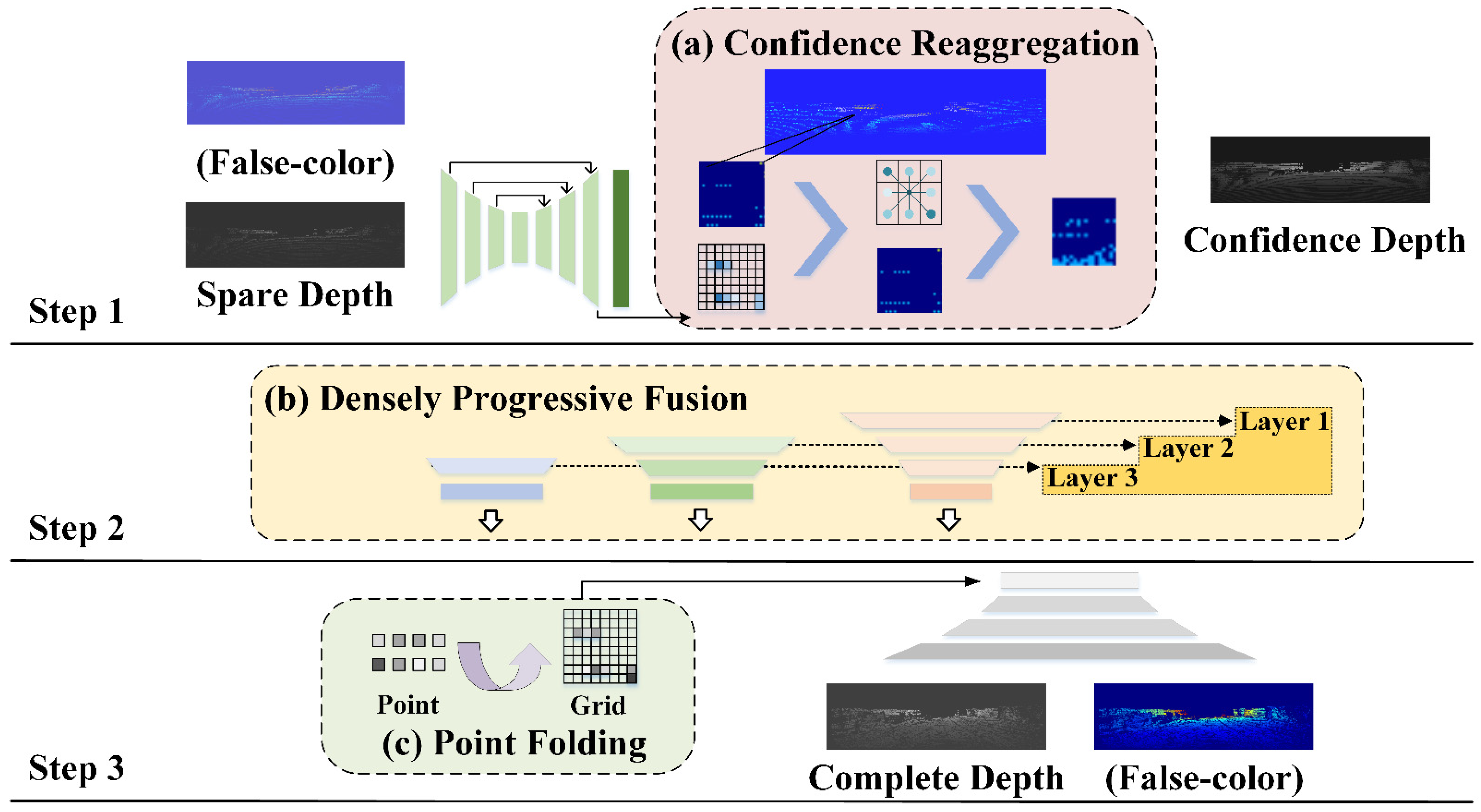
Figure 1. The overall structure of the network. Our network is divided into three steps: confidence generation, deep coding, and deep decoding, which are identified by three long lines from top to bottom. Firstly, we generate a confidence depth image based on the input sparse depth image by special convolution and aggregation methods. Then, the depth is gradually encoded according to confidence in the second step. Finally, the dense depth image is completed by the decoder. In addition, our ideas are marked in the figure. The pink dashed box (a) is the confidence re-aggregation module, which is described in Section 2.1. The yellow dashed box (b) is the dense progressive fusion module, which is described in Section 2.2. The green dashed box (c) is the point folding module, which is described in Section 2.3. The input and output are processed into false-color depth images for a clear presentation.
Remotesensing 14 04689 g001
Figure 2. The structure of the confidence re-aggregation module. We selected a square window in a feature image as an example to show it. (a) is the processing method of ordinary confidence. The confidence is obtained from the input. And then the input goes with the confidence to get the output. (b) is our processing method for confidence re-aggregation. We added a step in the middle. The confidence is re-aggregated based on the input.
Remotesensing 14 04689 g002
Figure 3. The schematic diagram of the dense progressive fusion module. There is a main road and two branches with different resolutions. The down arrows in the dashed box represent the down-sampling, and the up arrows are the up-sampling. After the fusion of multiple branches, the color of the feature is gradually deepened, which means that the effect is gradually better.
Remotesensing 14 04689 g003
Figure 4. The schematic diagram of the point folding module. The top line is a folding network for point cloud completion, which folds 2D random grid points into 3D shapes through neural network learning to complete point clouds. The bottom row is our proposed folding network for depth completion, which folds 1D random discrete points into 2D grid points through neural network learning to complete depth information.
Remotesensing 14 04689 g004
Figure 5. The complete results of our network on KITTI. (a) is the input sparse depth image. (b) is the completed depth image we output. (c) is the ground truth.
Remotesensing 14 04689 g005
Figure 6. The complete results of our network on NYU. (a) is the input sparse depth image. (b) is the completed depth image we output. (c) is the ground truth.
Remotesensing 14 04689 g006
Figure 7. The effects of the confidence re-aggregation module. (a) is the input sparse depth image and (b) is the ground truth. (c) is the completion effect without confidence re-aggregation module and its false-color image is (e). (d) is the completion effect without the confidence re-aggregation module and its false-color image is (f). The red circle on the left is the gap between the man and the handlebars. The red line on the right is the curvature of the backs of people, bikes, and wheels.
Remotesensing 14 04689 g007
Figure 8. The effects of the dense progressive fusion module. The image from the previous frame is shown in the left box, and the image from the contrast frame is shown in the right box. (a) is the ground truth. (b) is the output before joining the module. (c) is the output after joining the module. Their lower right corner is their false-color image.
Remotesensing 14 04689 g008
Figure 9. The effects of the point folding module. (a,c) are the results without point folding modules. (b,d) are the results of somewhat folded modules.
Remotesensing 14 04689 g009
Table 1. Comparisons to other methods without RGB image guidance on KITTI. The bold numbers are the best.
SI-Net [19]NCNN [22]IP-Basic [2]S2D++ [9]PNCNN [25]EIR-Net
MAE481.27360.28302.60288.64251.77225.70
IMAE1.781.521.291.351.051.02
RMSE1601.331268.221288.46954.36960.051061.75
IRMSE4.944.673.783.213.373.77
Time (s)0.010.01-0.040.020.02
Table 2. Comparisons to other methods on NYU. The bold numbers are the best.
TGV [37]RGB-d [38]S2D [9]NCNN [22]SPN [24]PNCNN [25]EIR-Net
RMSE0.6350.2280.2300.1710.1620.1440.142
ABSREL0.1230.0420.0440.0260.0270.0210.020
δ181.997.197.198.398.598.898.8
δ293.099.399.499.699.799.899.8
δ396.899.799.899.999.999.999.9
Table 3. The ablation experiments of the confidence re-aggregation module. The bold numbers are the best.
ModelOriginal+CR(TC)+CR(AS*)+CR(AS)
MAE227.416227.581226.786226.647
MSE1,274,874.1181,298,745.8421,281,756.1621,270,920.852
RMSE1065.5041074.6161067.3301063.893
IMAE1.020.980.990.97
IRMSE13.8215.96113.3515.763
Time0.0140.0170.0170.017
Table 4. The ablation experiments of the dense progressive fusion module and the point folding module. The bold numbers are the best.
ModelMAERMSEIMAEIRMSEδ1δ2δ3Time
None226.6471063.8930.975.76399.59499.84599.9210.017
DPF(1)226.2661066.0311.0622.62299.59599.84599.9210.018
DPF(2)225.8711063.6241.075.36399.59599.84699.9210.020
+P-Folding225.7031061.7451.023.77499.60099.84699.9220.020
Publisher’s Note: MDPI stays neutral with regard to jurisdictional claims in published maps and institutional affiliations.