A Comprehensive Study on Factors Affecting the Calibration of Potential Evapotranspiration Derived from the Thornthwaite Model

Abstract

Potential evapotranspiration (PET) is generally estimated using empirical models; thus, how to improve PET estimation accuracy has received widespread attention in recent years. Among all the models, although the temperature-driven Thornthwaite (TH) model is easy to operate, its estimation accuracy is rather limited. Although previous researchers proved that the accuracy of TH-PET can be greatly improved by using a limited number of variables to conduct calibration exercises, only preliminary experiments were conducted. In this study, to refine this innovation practice, we comprehensively investigated the factors that affect the calibration performances, including the selection of variables, seasonal effects, and spatial distribution of Global Navigation Satellite System (GNSS)/weather stations. By analyzing the factors and their effects, the following conclusions have been drawn: (1) an optimal variable selection scheme containing zenith total delay, temperature, pressure, and mean Julian Date was proposed; (2) the most salient improvements are in the winter and summer seasons, with improvement rates over 80%; (3) with the changes in horizontal (2.771–44.723 km) and height (1.239–344.665 m) differences among ten pairs of GNSS/weather stations, there are no obvious differences in the performances. These findings can offer an in-depth understanding of this practice and provide technical references to future applications.

1. Introduction

As a crucial meteorological parameter, potential evapotranspiration (PET) represents the maximum amount of water that would be evapotranspirated if a sufficient water source were available [1,2]. It is accepted that the evapotranspiration process is controlled by energy exchange at the vegetation surface, which is thus greatly limited by the energy amount [3]. From the aspect of synoptic meteorology, the factors of wind, air and surface temperature, humidity, and insolation all intensively affect the values of PET [4]. From the perspective of actual application, PET is generally required to assess aridity, irrigation water demand, and ground water recharge; calculate the water requirements of crops and landscape plants; and conduct hydrological cycle analysis and drought monitoring. Specific to the extending application of operational drought monitoring, PET is employed in the calculation of various types of drought monitoring indices, e.g., the Standardized Precipitation Evapotranspiration Index [5], the Palmer Drought Severity Index [6], and the Relative Moisture Index [7]. These also further highlight the importance of improving and guaranteeing the estimation accuracy of PET. Generally, the PET value is estimated using empirical models. On the basis of the adoption of different input variables and assumptions, the empirical models available in previous studies can be broadly categorized as fully physically based, semi-physically based, and black-box models [2,8]. The first type mainly accounts for mass and energy conservation principles; the semi-physically based models address either mass or energy conservation; the latter ones are developed based on the advanced neural network technique, genetic algorithm, or empirical relationships [9,10,11]. Among various types of empirical models, the most frequently used models are the Penman–Monteith (PM) [12] and Thornthwaite (TH) [13] models. A physically based model highly recommended by the Food and Agriculture Organization of the United Nations [3], the PM model takes a hypothetical crop canopy as the reference, and fully considers the influences brought by various types of variables, including temperature, humidity, wind speed, dew point temperature, sunshine duration, and radiation [14,15]. Through the complete process, the accuracy of PM-derived PET (hereafter PM-PET) can be effectively ensured. Moreover, since the actual evapotranspiration cannot be measured, the PM-PET time series is often taken as the reference to evaluate the PET values estimated using other models. However, the use of a large number and types of variables also makes the calculation process much more complicated. Furthermore, these variables are not always prepared or able be adequately obtained at any weather station; thus, the use and popularization of the PM model is greatly limited. Regarding the TH model, it is a temperature-based model, which only adopts the variables of temperature as well as the site latitude of the weather station to determine PET values (hereafter TH-PET). Based on its simple calculation mechanism, the TH model has wider applicability in comparison to the PM model [5]. From the other facet of the TH model, it is also because this model only takes into account the effects brought by numbered variables, the accuracy of TH-PETs is not as high as its corresponding PM-PETs [16,17,18,19]. Therefore, how to effectively improve the accuracy of TH-PET has received widespread attention over the past few decades.

Through years of research, several previous studies have already confirmed that the accuracy of TH-PETs can be greatly improved by using a limited number of atmospheric variables to conduct certain calibration exercises [20,21]. For example, Zhao et al. [22] proposed a concept that the accuracy of TH-PET can be improved through calibration by using the variables of temperature and precipitable water vapor (PWV). Ma et al. [23] also used the Global Navigation Satellite System (GNSS) and meteorological data collected in Yunnan Province to develop a modified composite index, which was then used to further improve the accuracy of a meteorological drought monitoring index. It is noteworthy that the use of a limited number of atmospheric variables in the calibration practice is to continue carrying forward the advantages of easy operation, wide comprehension, and calculation simplicity embodied in the TH model. Another phenomenon that can be found from the previous studies is that apart from commonly used weather variables, the atmospheric products, e.g., PWV and zenith total delay (ZTD) retrieved from the GNSS sounding technique, also play a vital role in the calibration process. The use of these variables is mainly based on its advantageous characteristics of high accuracy, high spatial and temporal resolution, 24-hour operability, and all-weather capability [24,25,26,27,28,29]. From another perspective, the atmospheric humidity conditions (especially the variations in water vapor), which are closely linked with the estimation of PET, can also be better reflected by PWV and ZTD estimates to some extent. Based on all these, the feasibility, effectiveness, and advantages of applying GNSS-derived products to serving the meteorological community has been thoroughly confirmed over the past few years [30,31,32,33,34]. However, it should be admitted that only preliminary experiments were conducted in those previous studies, which did not take those crucial factors affecting the calibration performances of TH-PET into deep consideration, and there many issues need to be addressed to further refine this type of application. For example, in [21,22], the variables of ZTD/temperature and PWV/temperature were simply used to carry out calibration exercises. Although great calibration performances were obtained, those studies lack further investigations of whether the use of other variables may also provide positive contributions to the final output. Moreover, while it is well known that different seasons have different atmospheric conditions, those studies only took data over a long period to conduct experiments, which did not further evaluate the calibration differences in different natural seasons.

The aim of this study is therefore to conduct comprehensive investigations of some critical factors that greatly affect the calibration performances of TH-PET estimates. The factors concerned in this study include the selection of variables, the seasonal calibration differences, and the spatial distribution of weather/GNSS stations. Based on the research status stated above, the choice of these factors is mainly because the first determines how to select optimal and effective variables to participate in the calibration process, and the other two are regarded as the crucial in the temporal and spatial domains, respectively. Apart from the comprehensive investigations conducted, some of the main innovations are also contained in the selection of variables adopted in the analyses. To be specific, the GNSS and weather variables chosen in this study include GNSS-derived ZTD (named GNSS-ZTD in this study), temperature, and pressure. The first innovative practice lies in the use of ZTD rather than PWV (in comparison to [22]); the reasons for this choice mainly include the following. (1) This practice can avoid a possible degradation in the accuracy caused by errors introduced from the use of meteorological variables in the conversion process from ZTD to PWV. (2) Various studies have also confirmed that the time series of ZTD and PWV have quite similar variation trends [35,36], indicating that the two variables may have analogical influences on the linear calibration exercises. The second novelty lies in the fact that the statistical parameter of mean Julian Date (MJD), reflecting the time-varying characteristics of other atmospheric variables, was first introduced to an application of this type. The primary reasons for incorporating this parameters include that (1) the MJD is a common variable adopted in the PM model, which has the ability to reflect the effects brought by insolation. Thus, the additional use of this variable would help to fill in the gaps of estimating PET using the TH model, in comparison to the physically based PM model. (2) Many previous studies [37,38,39] have already confirmed that time-varying variables (e.g., hour-of-day and day-of-year) can exert great positive influences on final performances. (3) It is proved that pressure, temperature, ZTD, and PET possess obvious annual, seasonal, and even diurnal variation features, which can all be effectively manifested by MJD. Therefore, the adoption of MJD in this study has significant potential to further improve the accuracy of calibrated TH-PET. Based on all the comprehensive investigations with the above-mentioned innovation practices conducted in this study, the research findings can offer an in-depth understanding of this practice and also provide technical references for future applications.

2. Data Acquisition

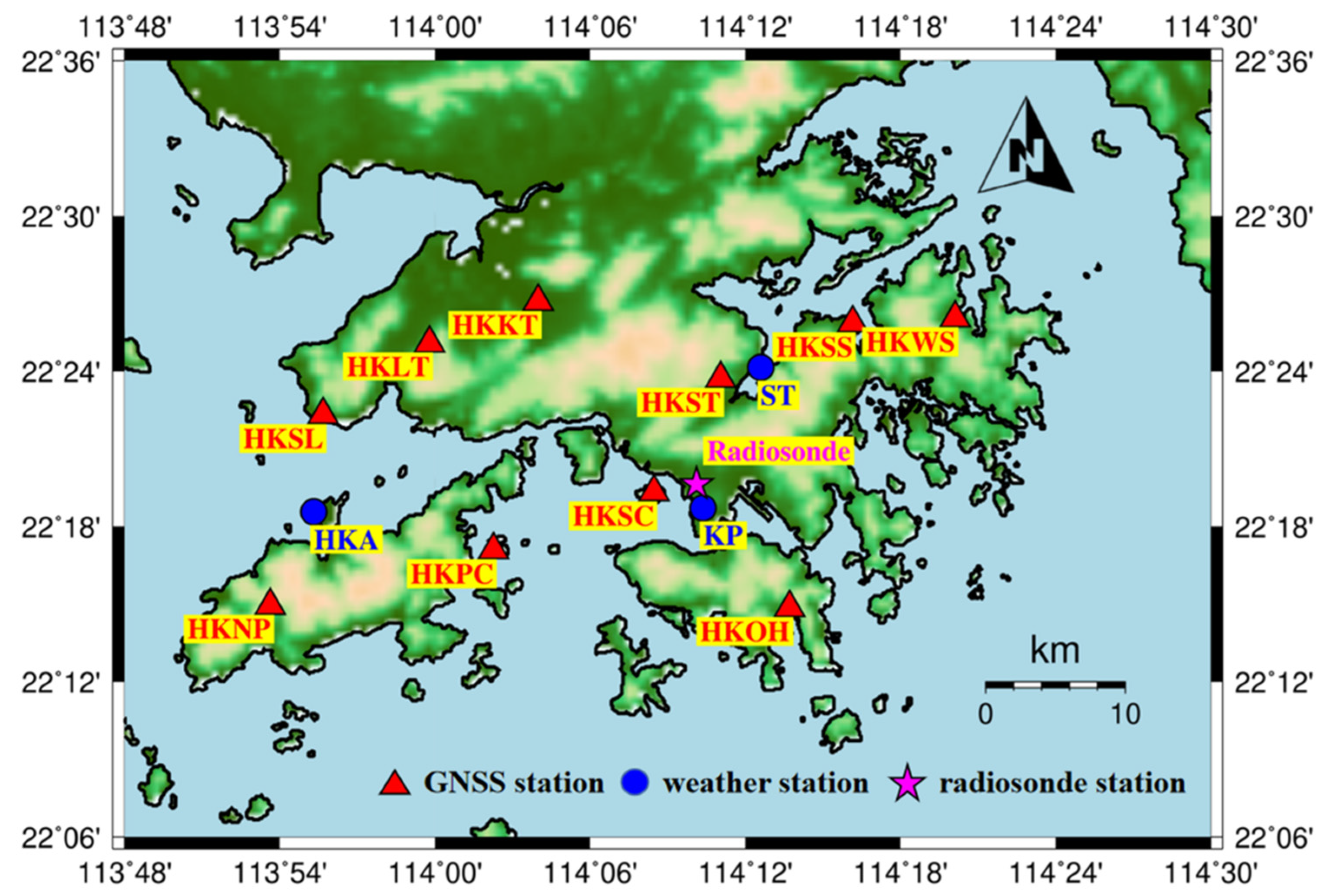
2.1. Selection of Study Region and Period

In this study, on account of the main aspects of climate conditions, research demands, and data integrity/availability, the Hong Kong region was selected as the experimental area. (1) Climate conditions: The Hong Kong region, which possesses typical sub-tropical climate features [40], has generally experienced various types of extreme climate phenomena and severe weather events over the past few decades, especially in its summer seasons [41,42,43]. (2) Research demands: According to the reports released by the Hong Kong Observatory [44] and the Intergovernmental Panel on Climate Change [45], more frequent and devastating climate and weather extremes, e.g., heavy precipitation, meteorological drought, and typhoon, will strike this area in the coming years. This highlights a pressing research demand to effectively monitor all these extreme phenomena in this area. Fortunately, as suggested before, research on improving the accuracy of PET estimates (as in this study) may then assist in the calculation of indices for drought monitoring and promote the analysis of hydrological processes and parameters. (3) Data integrity/availability: This is another crucial issue that cannot be ignored, especially for studies addressing climate problems. To ensure the reliability and credibility of the research outputs from this study, the experimental data including GNSS-ZTD, temperature, pressure, solar radiation, dew point temperature, sunshine duration, relative humidity, and wind speed collected over a 14-year period from 2008 to 2021 were all adopted in the estimation and calibration of PET values. The use of this long-term period is to effectively capture the variation trends of different atmospheric variables, and grasp the intrinsic nature of this application. In the selected study region, these variables can be simply obtained/retrieved from GNSS tracking stations (from the Hong Kong Continuously Operating Reference Stations network) and operational weather stations. To be more specific, the GNSS stations adopted in this study include the HKKT, HKLT, HKNP, HKOH, HKPC, HKSC, HKSL, HKSS, HKST, and HKWS stations. The Hong Kong International Airport (HKA), King’s Park (KP), and Sha Tin (ST) weather stations were selected for collecting meteorological data. According to statistics, the integrity rates of ZTD and meteorological measurements over the whole 14-year study period were 99.1% and 98.8%, respectively. Therefore, the use of these data with better integrity could effectively ensure the reliability and reasonability of the conclusions resulting from the following experiments. Figure 1 and

Table 1. Coordinate information of the selected GNSS and weather stations.

Station ID		Latitude (°)	Longitude (°)	Height (m)
GNSS station	HKKT	22.45	114.07	34.54
	HKLT	22.42	114.00	125.90
	HKNP	22.25	113.89	350.67
	HKOH	22.25	114.23	166.38
	HKPC	22.29	114.04	18.09
	HKSC	22.32	114.14	20.20
	HKSL	22.37	113.93	95.27
	HKSS	22.43	114.27	38.68
	HKST	22.40	114.18	258.69
	HKWS	22.43	114.34	63.76
Weather station	HKA	22.31	113.92	6.00
	KP	22.31	114.17	65.00
	ST	22.40	114.21	6.00

illustrate the spatial distribution and detailed coordinate information of the thirteen stations adopted in this study, respectively. Note that the only radiosonde station employed in the study region was also plotted in Figure 1. Its sounding profiles can be used as the reference to test the accuracy of GNSS-derived atmospheric products.

2.2. Retrieval of GNSS-ZTD

In this study, as mentioned in Section 1, to avoid introducing additional error sources in the conversion from ZTD to PWV, as well as to enhance the spatial resolution in the selection of GNSS stations, only the ZTD estimates retrieved from the GNSS observations were adopted in the following analyses. The retrieval of ZTD time series over the 14-year study period at the selected ten stations was conducted by using Bernese GNSS Software Version 5.2 [46]. The detailed data processing strategies were generally the same as those adopted in our previous studies [35], including the double-difference approach, the elevation angle cutoff of 3°, the Vienna Mapping Function 1, and the operational International GNSS Service Finals clocks and orbits [47,48]. Regarding temporal issues, a 27-hour observation window was selected, and the temporal resolution of ZTD estimates as well as estimation spacing were both set to 5 min [49,50]. In addition, the relativistic delays, the effects of the solid Earth pole tide, ocean pole tide, and phase wind-up were all modeled in line with the International Earth Rotation and Reference Systems Service Conventions 2010 [51]. With the adoption of these strategies, the accuracy of GNSS-derived atmospheric products was fully validated in different study areas over the past few years [52,53,54]. Specific to the Hong Kong region, in our previous studies [33,35], the accuracy of ZTD and PWV were tested and assured using sounding profiles as the reference, effectively meeting the requirements for operational use in the meteorological community.

2.3. Meteorological and Time-Varying Variables

Prior to using the obtained GNSS-ZTD time series as a key factor to calibrate PET values, the PETs should be predetermined based on the empirical TH and PM equations (data obtained from the latter was taken as the reference for evaluation). As suggested by Thornthwaite [13] and Monteith [12], the data types of meteorological variables needed in the whole estimation process generally include temperature, pressure, solar radiation, dew point temperature, sunshine duration, relative humidity, and wind speed [3,19,55]. In this study, all the required monthly and diurnal meteorological data over the 14-year period from 2008 to 2021 can be easily collected from the Hong Kong Observatory at the three operational weather stations, i.e., HKA, KP, and ST.

As mentioned in Section 1, apart from all the aforementioned variables, the time-varying variable of MJD was also adopted in the experiments, which has the potential to reflect the temporal variations in the above variables as well as PET. It is well known that the conventional Julian Date is counted per day, i.e., each date has a certain value (in the range 1–366). However, to be in line with the mechanism of the TH equation, which is designed to calculate monthly PET values, the MJD was calculated and utilized in this study. As its name suggests, the MJD is actually the average value of all the Julian Dates in a certain month. For example, the MJD value of January is 16, which is the mean value of 1–31. With the use of this simple computational strategy, the MJD value for each month in each year can be easily obtained.

3. Methodology

On the basis of the whole procedure, the methodologies adopted in this study can be divided into the following two parts. The first one is to estimate PET values using the TH and PM equations, and the second is to calibrate the obtained PET values using GNSS and meteorological products.

3.1. Estimation of PET

3.1.1. Thornthwaite Equations

As a type of temperature-driven method, only temperature is required in the estimation of PETs using the empirical TH equations, which manifests its main advantages of easy operation, high efficiency, and wide applicability. It is also noted that in some calculation methods, the factor of latitude (reflecting duration of day) is also incorporated. In this study, as suggest by the China Meteorological Administration [56], the general equation for estimating TH-PET can be expressed as:

$$PE{T}_T=16.0\times {[\left(10\times T_i\right)/H]}^A,$$

(1)

where $PE{T}_T$ represents the obtained TH-PET estimate, in mm. Since this model was originally designed for calculating monthly PET values according to [13], T_i and its subscript i denote the monthly mean temperature (°C) and the index of the twelve months (ranging from 1 to 12), respectively. It is worth mentioning that the above equation is only available for the situations when T_i is above 0 °C; while in the other cases (i.e., when T_i is less than or equal to 0 °C), the values of $PE{T}_T$ are regarded as zero. H denotes the annual heat index, the calculation of which should be conducted by summing up all the monthly heat indices in a certain year using the equation below:

$$H={\sum }_{i=1}^{12}{H}_i={\sum }_{i=1}^{12}{\left(T_i/5\right)}^{1.514},$$

(2)

where H_i is the monthly heat index; the subscript i represents the index of each month. Regarding the notation of A shown in Equation (1), it denotes a “constant” coefficient. Since the coefficient value is highly dependent on that of the annual heat index, with the obtained annual heat index, the coefficient can be easily calculated using Equation (3). In other words, given that the annual heat index of a certain year is obtained, the coefficient A can be recognized as a constant value during the year.

$$A=6.75\times {10}^{-7}{H}^3-7.71\times {10}^{-5}{H}^2+1.792\times {10}^{-2}H+0.49,$$

(3)

Overall, with the use of temperature measurements, all the other variables (H_i, H and A) contained in the estimation of TH-PET can be calculated from the use of T_i based on the above equations. This phenomenon further corroborates the fact that the TH model is driven by temperature values. Therefore, with the obtained monthly mean temperature collected at the three weather stations, the TH-PET series over the 14-year study period at each site can be calculated.

3.1.2. Penman–Monteith Equations

The Penman–Monteith model is the other operational way to estimate PET values. It is known that the PET estimates derived from this method are generally regarded as the “true” values, which are often adopted as the reference to evaluate those calculated from other equations (e.g., the TH model). However, it can be seen from its principal formula that the PM model requires more types of meteorological data than the TH model, and its computational procedure is also more complicated [3,56]:

$$PE{T}_P=\frac{0.408\Delta \left(R_n-G\right)+\gamma \frac{900}{T_i+273.16}{u}_2\left(e_s-e_a\right)}{\Delta +\gamma \left(1+0.34u_2\right)},$$

(4)

where $PE{T}_P$ represents the PM-PET estimate, in mm; $\Delta$ and $\gamma$ denote the slope of the water vapor curve (kPa·°C⁻¹) and a psychrometric constant (kPa·°C⁻¹), respectively; $R_n$ and $G$ are the surface net radiation (MJ·m⁻²·d⁻¹) and soil heat flux (MJ·m⁻²·d⁻¹), respectively; T_i represents the mean temperature measurement (°C); u₂ is the 2 m wind speed, in m·s⁻¹; $e_s$ and $e_a$ denote the saturation and actual vapor pressure, in kPa, respectively. In addition, the constant values of 900 and 0.34 represent the coefficient and the wind coefficient for the reference crop. To be more specific, the following equations are adopted to calculate the saturation and actual vapor pressure:

$$e_a=0.6108\times exp\left[\frac{17.27\times T_{dew}}{T_{dew}+237.3}\right],$$

(5)

$$e_s=0.3054\times \{exp\left[\frac{17.27\times T_{max}}{T_{max}+237.3}\right]+exp\left[\frac{17.27\times T_{min}}{T_{min}+237.3}\right]\},$$

(6)

where T_dew represents the dew point temperature, in °C; T_max and T_min denote the highest and lowest temperature estimates (°C), respectively. Regarding the psychrometric constant, its determination needs the incorporation of pressure measurement (denoted by P, in kPa) using the formula below:

$$\gamma =0.665·{10}^{-3}\times P,$$

(7)

In addition, since PM-PETs were used to evaluate TH-PETs to be in line with the estimation of monthly PET values, the simplified equation outlined below can be obtained to calculate the soil heat flux $G$:

$$G=0.14\times \left(T_{month, i}-T_{month, i-1}\right),$$

(8)

Where $T_{month, i}$ and $T_{month, i-1}$ denote the monthly mean temperatures (°C) of the i-th and its previous (denoted by (I − 1)) month, respectively; the subscript i has the same meaning as that shown in Equation (1). Due to limited space in this article, more details regarding the computational mechanism of the PM model can be found in [3,56,57]. Therefore, with the use of the PM model, the PM-PET time series over the study period at the selected operational weather stations can also be accurately determined.

3.2. Calibration of PET

According to previous statements, after the estimation of PET values using the above two models, the second process is to calibrate the TH-PET estimates using various types of GNSS and meteorological products. This procedure can be separated into the following three steps:

• Calculation of PET differences between PM-PET and TH-PET estimates:

$$PE{T}_{diff}=PE{T}_P-PE{T}_T,$$

(9)

where $PE{T}_P$ and $PE{T}_T$ represent the PET estimates obtained from the empirical PM and TH models, respectively. $PE{T}_{diff}$ denotes the PET difference between the two sets of PETs (mm). The calculation of PET differences is to test the estimation errors contained in the TH-PET series compared to those obtained from the PM model, which are recognized as the “true” values, as stated earlier.

2.

Calibration of TH-PET estimates using GNSS and meteorological variables:

$$PE{T}_{cal}=a_1{X}_1+a_2{X}_2+a_3{X}_3+\dots +a_n{X}_n+b,$$

(10)

where $PE{T}_{cal}$ represents the calibrated residual of the PET estimates (mm); X₁, X₂, X₃,..., X_n denote various types of atmospheric products; a₁, a₂, a₃,..., a_n are the coefficient values of all the selected variables; b is the intercept of the linear calibration equation; the subscript n is the number of variables adopted in the calibration process. It can be seen from the equation that the values of all the coefficients and intercept should be predetermined over a certain study area so as to put into operation in future applications. Actually, the determination of these values is more like the training process in existing machine learning-based models, especially the supervised learning technique [31,38,39,58]. In the context of this application, the PET differences as well as all the required atmospheric variables over a long-term period should be used to map the corresponding relation between the input–output data pairs. Among them, the PET differences obtained from the previous step using Equation (9) are regarded as the “desired output”, with which the TH-PET values can be accurately calibrated; different types of atmospheric variables are the “input” of Equation (10) (denoted by a₁, a₂, a₃,..., a_n). In this study, the whole datasets over the 14-year period at each station were divided into two parts: data over the 12-year period from 2008 to 2019 were used to determine the coefficients and intercept, and thus to construct the specific calibration equation at each weather station; data over the other 2-year period from 2020 to 2021, which can be regarded as an independent set of data, were used to test the performances resulting from the established equations. In addition, as mentioned in Section 1, to continue demonstrating the advantages contained in the TH model, we only utilized a limited number of variables, which are also readily accessible and commonly used, in the following section.

3.

Calculation of a new set of TH-PET values over the whole period:

$$PE{T}_{imp}=PE{T}_T+PE{T}_{cal},$$

(11)

where $PE{T}_{imp}$ represents the TH-PET estimate that has already been calibrated (mm), which is the sum of the original TH-PET value $PE{T}_T$ and the calibrated residual $PE{T}_{cal}$. It it noteworthy that this process can also be divided into two parts in accordance with the previous step. For the first part regarding the construction of the calibration equation using data over the period 2008–2019, the results obtained by comparing the new set of PET estimates with the PM-PETs are generally called “fitting results”. This is because PET differences (obtained from Equation (9)) over the 12-year period were adopted as the “desired outputs” to conduct the regression analysis. For the other part, i.e., the verification of the constructed calibration equation using data over the 2-year period 2020–2021, the comparison results are called “verification results”. Moreover, in the testing procedure, the metrics of correlation coefficient (r), bias, root mean square (RMS) error, and Nash-Sutcliffe Efficiency (NSE) [59,60] were all adopted to quantitatively evaluate the performances resulting from each experimental schemes designed in this study. The computational mechanisms of these metrics are outlined as follows:

$$\mathrm{Bias}={\sum }_{i=1}^n\left(X_i-Y_i\right)/n,$$

(12)

$$\mathrm{RMS}=\sqrt{{\sum }_{i=1}^n{\left(X_i-Y_i\right)}^2/n},$$

(13)

$$r=\frac{{\sum }_{i=1}^n\left[\left(X_i-\overline{X}\right)\times \left(Y_i-\overline{Y}\right)\right]}{\sqrt{[{\sum }_{i=1}^n{\left(X_i-\overline{X}\right)}^2\times {\sum }_{i=1}^n{\left(Y_i-\overline{Y}\right)}^2]}},$$

(14)

$$\mathrm{NSE}=1-\frac{{\sum }_{i=1}^n{\left(X_i-Y_i\right)}^2}{{\sum }_{i=1}^n{\left(X_i-\overline{X}\right)}^2},$$

(15)

where the subscripts n and i denote the total number and the index of the samples in the obtained PET time series. The PET time series obtained from the PM model is regarded as the reference to evaluate the accuracy of calibrated/non-calibrated TH-PETs in this study; thus, $X_i$ and $Y_i$ are the i-th PM-PET and TH-PET values obtained at different stations. $\overline{X}$ and $\overline{Y}$ denote their respective average values over the whole series.

Therefore, with all the methodologies, the PET estimates can be easily obtained based on the empirical TH and PM models. Then, through a comprehensive calibration process using different types of meteorological variables, the accuracy of TH-PETs can be further improved. The following section examines the key factors that greatly affect the calibration performances.

4. Investigation of Factors Affecting the Calibration Performance of PET Estimates

In this study, several crucial factors that affect the calibration performance of TH-PETs were comprehensively investigated, including the selection of variables for calibration, seasonal calibration effects, and the spatial distribution of GNSS and weather stations. We selected these three factors mainly because the first is one of the most important preparatory steps prior to conducting the calibration process, and the latter two are the core factors contained in the temporal and spatial domains. Their respective investigation findings are presented in the following subsections.

4.1. Selection of Variables for Calibration

Although the calibration practice of TH-PETs using temperature, ZTD, PWV, and other types of atmospheric variables were proved to be effective in previous studies [20,21,22], there is a lack of a specific principle for the selection of variables involved in the calibration of TH-PET estimates in the existing literature. In this study, to thoroughly test the performances resulting from different combinations of variables, eight experimental schemes with the use of ZTD, MJD, temperature, and pressure were designed, as shown in

Table 2. Eight experimental schemes for investigating the calibration performances resulting from different combinations of atmospheric variables. (Temperature and pressure are denoted by T and P, respectively.)

Scheme No.	Variables	No. of Variables
1	T, P	2
2	T, ZTD	2
3	P, ZTD	2
4	T, P, ZTD	3
5	T, P, MJD	3
6	T, ZTD, MJD	3
7	P, ZTD, MJD	3
8	T, P, ZTD, MJD	4

. The reasons for the utilization of ZTD and MJD were stated earlier, and the selection of temperature and pressure is mainly because they are the most commonly used and easily accessible meteorological variables. From another aspect, apart from the required monthly mean temperature measurements, only two types of variables (ZTD and pressure) were additionally used (note that MJD is a statistical concept that can be simply calculated), which conforms to the advantages of the TH model.

It is known that it is unconvincing and unreasonable to conduct the calibration practice using only one type of variable. Therefore, with the use of two to four types of variables, all the possible experimental schemes are listed in this table. As mentioned in Section 3, the datasets over the periods 2008–2019 and 2020–2021 at the three selected weather stations (HKA, KP, and ST) were used to construct and test the calibration functions. Since the GNSS sites are dispersedly distributed in the study region, to conduct a more reasonable analysis and to effectively guarantee the adaptability of the ZTD time series, as well as to avoid introducing errors on account of spatial distances, the above experiments only adopted the ZTD values obtained from the nearest GNSS stations to each of the three weather stations. This practice is similar to those adopted in our previous studies [33,35]. By calculating and analyzing the distances between each pair of GNSS and weather stations, three GNSS stations were selected for their corresponding “co-located” weather stations, i.e., three pairs of GNSS/weather stations were adopted (HKA-HKSL, KP-HKSC, and ST-HKST). In addition, to evaluate the calibration performances resulting from the eight schemes, the original TH-PETs over the same period were taken as the benchmarks. Because there is no calibration conducted in this case, the results could assess whether improvements have been made by using the eight schemes.

Table 3. Comparison of the average fitting and verification results obtained from each scheme at the three pairs of co-located GNSS/weather stations.

Scheme No.	Calibration Variable	Fitting Results (2008–2019)				Verification Results (2020–2021)
		Bias (mm)	RMS (mm)	r	NSE	Bias (mm)	RMS (mm)	r	NSE
1	T P	0	8.03	0.919	0.852	1.98	10.40	0.919	0.723
2	T ZTD	0	7.51	0.938	0.881	2.35	8.63	0.937	0.802
3	P ZTD	0	7.82	0.938	0.875	0.07	8.85	0.936	0.798
4	T P ZTD	0	7.33	0.947	0.897	1.92	8.30	0.938	0.814
5	T P MJD	0	7.86	0.923	0.855	1.61	10.05	0.923	0.731
6	T ZTD MJD	0	7.34	0.944	0.891	2.13	8.39	0.939	0.806
7	P ZTD MJD	0	7.44	0.946	0.890	0.03	8.56	0.938	0.808
8	T P ZTD MJD	0	6.95	0.952	0.904	1.35	8.13	0.940	0.824
9	None	2.59	34.42	0.919	−0.512	4.07	39.23	0.902	−1.432

lists the average fitting and verification results, including the four metrics of bias, RMS, NSE, and correlation coefficient, obtained from each scheme at the three pairs of stations.

It can be clearly seen from Table 3 that compared with the results obtained from Scheme 9, the fitting and verification performances resulting from the other eight schemes (with the additional calibration process) were all greatly improved, no matter what types of variables were adopted. Among the eight experimental schemes, Scheme 8 outperformed the others considering the metrics of RMS, correlation coefficient, and NSE, in which the variables of temperature, pressure, ZTD, and MJD were all simultaneously utilized. From a statistical perspective, the improvements in the average fitting and verification RMS results made by using Scheme 8, in comparison to those from the use of Scheme 9, were 27.47 mm (79.8%) and 31.1 mm (79.3%), respectively. Specific to the three pairs of co-located stations, the improvements in the fitting and verification results even reached 81.5% (KP-HKSC) and 80.5% (ST-HKST), respectively. Furthermore, the calculation of drought monitoring indices is closely linked with the (normal) distribution of the differences between precipitation and PET [56]; thus, the higher the correlation coefficient values, the more accurate the indices. The rises in the correlation coefficient values may also promote the determination of more accurate drought monitoring indices using the calibrated TH-PET. Another phenomenon that can be observed is that after the whole calibration process, the bias values were all calibrated to zero (see the shaded column in Table 3). It is widely known that the data range for the metric of NSE is (−∞, 1]. In this study, the values of NSE nearer to 1 suggest that the estimation error variances are close to zero, i.e., the TH-PET time series is well-calibrated. In the situation of the calibrated TH-PET time series with an error covariance, this is considerably larger than the variance of the PM-PETs, and the resulting NSE values become negative. Based on the interpretation principles of NSE, it can be simply seen from Table 3 that great improvements have been made by conducting calibration exercises using the eight schemes, and the optimal results were derived from the use of Scheme 8 (with the NSE values of 0.904 and 0.824 in the fitting and verification stages, respectively).

To conduct a more detailed analysis, by comparing the statistical results obtained from these pairs of schemes (1 vs. 5; 2 vs. 6; 3 vs. 7; 4 vs. 8), it can be found that the additional use of MJD exerted a clearly positive influence on the final outputs, especially with respect to the correlation coefficient results. The comparing cases including (1 vs. 4) and (5 vs. 8) also obviously suggest that the ZTD time series may greatly improve the calibration performances. The RMS results in the two cases were reduced from 8.03 mm to 7.33 mm and from 7.86 mm to 6.95 mm, respectively. The positive influences brought by using temperature and pressure can also be reflected by comparing the results outlined above. Therefore, based on all the results shown in Table 3, together with the analyses carried out above, Scheme 8 was determined as the optimal one for the following experiments to investigate other factors affecting the calibration performances of TH-PETs.

4.2. Comparison of Seasonal Calibration Effects

After the selection of the most appropriate variables for conducting the calibration process, we further investigated a crucial factor contained in the temporal domain, i.e., the seasonal calibration effect. The datasets over the whole calibration period were separated into four groups in accordance with the four seasons: spring (March, April, and May), summer (June, July, and August), autumn (September, October, and November), and winter (December, January, and February). Then, the calibration performances in each season were statistically analyzed. To evaluate the calibrated results, as the practice conducted in Section 4.1, the performances obtained under the situation without the whole calibration process were also taken as the reference. In addition, to make an overall comparison,

Table 4. Comparison of the average seasonal differences between potential evapotranspiration (PET) time series estimated from the Penman–Monteith (PM) and Thornthwaite (TH) models at the three pairs of stations under the conditions of with and without calibration over the period 2008–2019.

Season	With Calibration (Scheme 8 in Table 3)				Without Calibration				Improvement Rate of RMS Result (%)
	Bias (mm)	RMS (mm)	r	NSE	Bias (mm)	RMS (mm)	r	NSE
Spring	9.49	9.34	0.935	0.596	12.84	27.10	0.778	−1.198	65.54
Summer	−2.06	5.48	0.856	0.668	−36.72	37.85	0.759	−6.704	85.52
Autumn	−2.68	6.24	0.933	0.824	−7.00	25.50	0.839	−0.582	75.52
Winter	−5.30	6.20	0.769	0.387	40.98	43.10	0.230	−14.874	85.61

lists the average differences between the two sets of PET time series calculated at the three pairs of GNSS/weather stations under the conditions of with and without calibration in the four seasons over the whole calibration period from 2008 to 2019. The use of data over the 12-year study period (rather than the whole 14-year period from 2008 to 2021) is because these data were carefully calibrated in the verification stage. With the adoption of these data, the performances resulting from with and without calibration can be better revealed. These results are presented in Figure 2 for a clear visual comparison.

Concerning the RMS and correlation coefficient values, which were obtained under the conditions of with and without calibration in the four different seasons, two phenomena can be clearly summarized. (1) Firstly, with respect to the original TH-PETs (under the circumstances of without the calibration process) at the three pairs of stations, the optimal results appeared in the seasons of autumn and spring, with their respective r/RMS results of 0.839/25.50 mm and 0.778/27.10 mm. The performances obtained in the other two seasons of summer (0.759/37.85 mm) and winter (0.230/43.10 mm) were rather worse. (2) Secondly, after a thorough calibration process, the RMS and correlativity results of the four seasons were all significantly improved. Regarding the improvement rate of those obtained RMS results (see the right column of the table), the highest improvement rate lies in the season of winter, to which the results obtained in the summer season was also similar (85.52% vs. 85.61%). Compared with these results, although the corresponding results in the spring and autumn seasons were relatively lower, the values of 65.54% and 75.52% in the respective two seasons were also considerable. Apart from these two types of metrics, even though the bias values only reflect the differences between the two sets of PET time series in different seasons, they were also reduced after the calibration. It is worth mentioning that the results obtained in the same season at the three stations were all with the same positive/negative signs. Although the bias values were all calibrated to zero over the 12-year calibration period from 2008 to 2019 (see the bold italic figures in Table 3), their seasonal bias values varied greatly. To be specific, after the calibration process, only the bias value for the spring is a positive value, indicating that the PM-PETs are generally larger than the calibrated TH-PETs, while the bias values for the other seasons are negative ones. Regarding the metric of NSE, although the values obtained for each season were generally lower than those shown in Table 3, they were all significantly improved after the whole calibration processes. Even in the winter season, the NSE values were improved from −14.874 to 0.387.

Overall, the calibration process can effectively improve the accuracy of TH-PETs obtained in each of the four seasons. Specifically, from the perspective of RMS results, the calibration process was proved to be the most effective for the PET estimates obtained in the seasons of winter and summer; from the perspective of correlativity, the optimal results were in the seasons of autumn and spring.

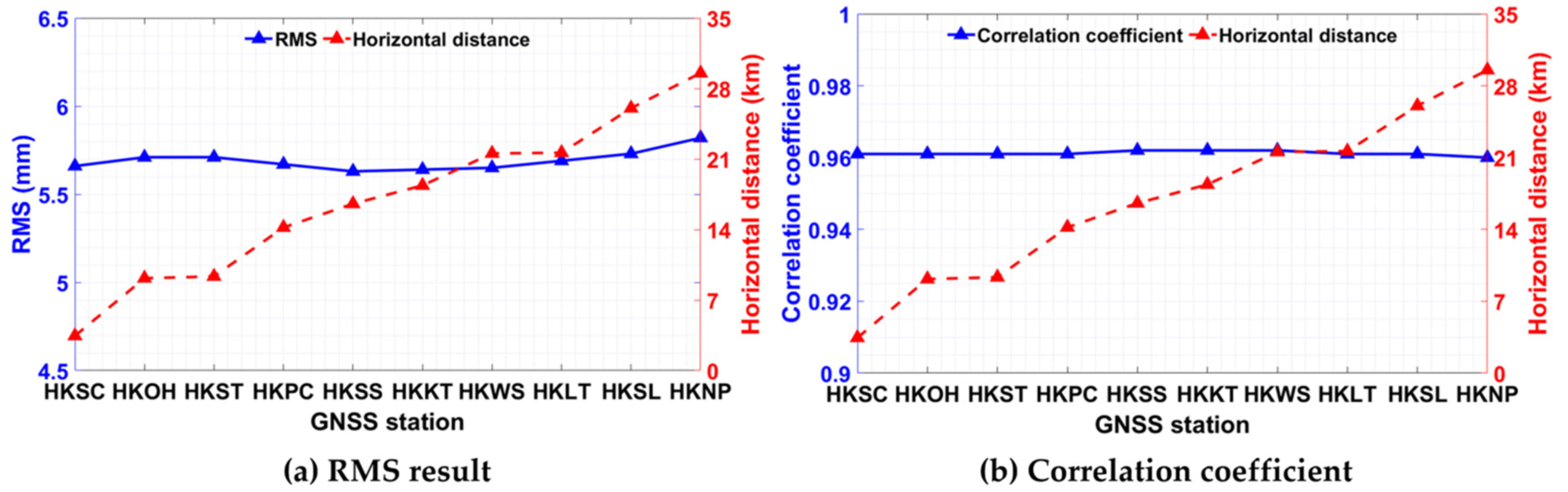
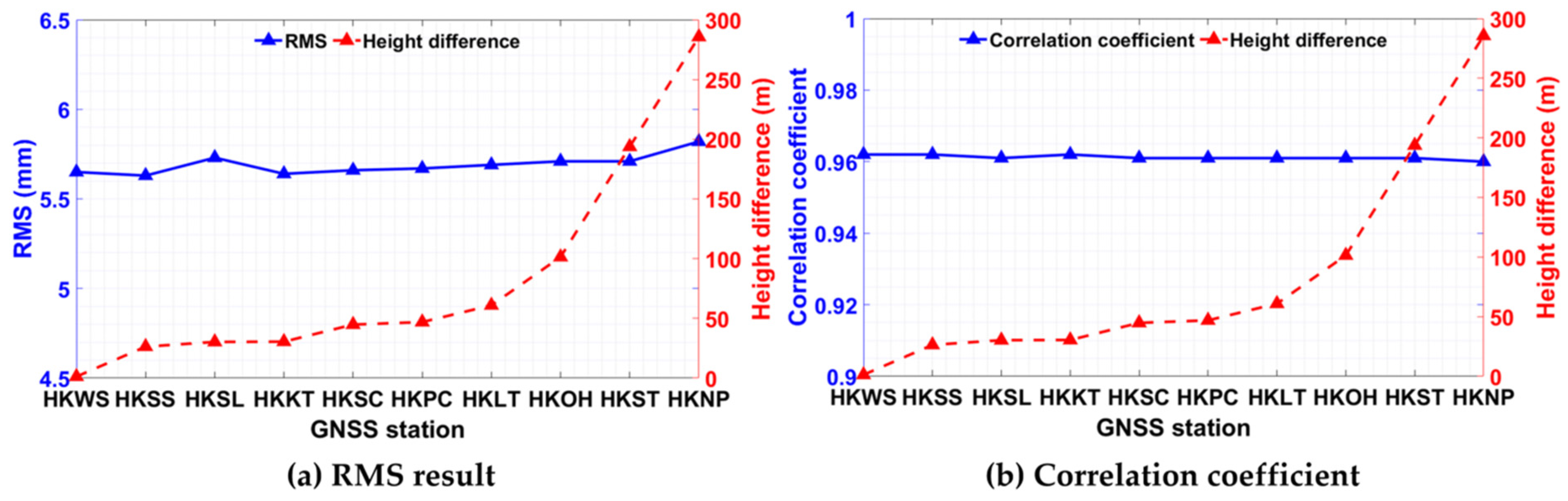
4.3. Spatial Distribution of GNSS and Weather Stations

Finally, regarding the spatial domain, it is important to determine the influences brought by the factor of the spatial distribution of GNSS and weather stations (i.e., the spatial distances between each pair of GNSS and weather stations) on the calibration performances of TH-PET. The motivation of investigating this factor mainly comes from the fact that ZTD and other types of meteorological variables are obtained from different sensing techniques at different locations. As shown in Figure 1, a total of ten GNSS stations were employed, and the ZTD time series over the whole study period at each station were all retrieved. According to Section 4.1, ZTD estimates have already been proven effective to calibrate TH-PET values; however, all of the previous experiments only used the GNSS and meteorological products obtained at the three pairs of co-located GNSS/weather stations to ensure their rationality. Therefore, determining whether the spatial distribution of GNSS and weather stations may have a remarkable effect on the calibration results of TH-PETs affects the feasibility and extension of this application in future practices. In this section, with the use of temperature and pressure measurements collected at the three weather stations (HKA, KP, and ST), as well as the time-varying variable of MJD, the retrieved ZTD values at each of the ten GNSS stations were used to calibrate the TH-PETs at the weather stations. Because the horizontal distances and height differences between each pair of GNSS and weather stations are different, the factor of spatial distribution is divided into two parts to separately investigate the influences brought by the differences in the horizontal and vertical directions. Therefore, by using the PM-PET values calculated at each weather station as the reference,

Table 5. Calibration performances of TH-PETs resulting from the temperature, pressure, mean Julian Date (MJD), and ten sets of zenith total delay (ZTD) time series at the three weather stations (HKA, KP, and ST) over the period 2008–2019. The horizontal distances between each pair of GNSS/weather stations are illustrated.

HKA Station				KP Station				ST Station
GNSS	Horizontal Distance (km)	RMS (mm)	r	GNSS	Horizontal Distance (km)	RMS (mm)	r	GNSS	Horizontal Distance (km)	RMS (mm)	r
HKSL	6.984	8.52	0.941	HKSC	3.443	5.66	0.961	HKST	2.771	6.66	0.955
HKNP	7.304	8.69	0.938	HKOH	9.166	5.71	0.961	HKSS	6.875	6.55	0.957
HKPC	12.228	8.49	0.941	HKST	9.343	5.71	0.961	HKSC	11.392	6.63	0.956
HKLT	14.315	8.48	0.941	HKPC	14.208	5.67	0.961	HKWS	13.366	6.57	0.956
HKKT	21.168	8.40	0.942	HKSS	16.555	5.63	0.962	HKKT	15.475	6.55	0.957
HKSC	22.599	8.48	0.941	HKKT	18.378	5.64	0.962	HKOH	17.319	6.65	0.955
HKST	28.610	8.54	0.940	HKWS	21.557	5.65	0.962	HKLT	22.005	6.62	0.956
HKOH	32.291	8.56	0.940	HKLT	21.623	5.69	0.961	HKPC	22.015	6.61	0.956
HKSS	38.193	8.42	0.942	HKSL	26.046	5.73	0.961	HKSL	29.191	6.63	0.956
HKWS	44.723	8.44	0.942	HKNP	29.533	5.82	0.960	HKNP	36.717	6.76	0.954

and

Table 6. Calibration performances of TH-PETs resulting from the temperature, pressure, MJD, and ten sets of ZTD time series at the three weather stations (HKA, KP, and ST) over the period 2008–2019. The height differences between each pair of GNSS/weather stations are illustrated.

HKA Station				KP Station				ST Station
GNSS	Height Difference (m)	RMS (mm)	r	GNSS	Height Difference (m)	RMS (mm)	r	GNSS	Height Difference (m)	RMS (mm)	r
HKPC	12.094	8.49	0.941	HKWS	1.239	5.65	0.962	HKPC	12.094	6.61	0.956
HKSC	14.204	8.48	0.941	HKSS	26.316	5.63	0.962	HKSC	14.204	6.63	0.956
HKKT	28.542	8.40	0.942	HKSL	30.267	5.73	0.961	HKKT	28.542	6.55	0.957
HKSS	32.684	8.42	0.942	HKKT	30.459	5.64	0.962	HKSS	32.684	6.55	0.957
HKWS	57.761	8.44	0.942	HKSC	44.796	5.66	0.961	HKWS	57.761	6.57	0.956
HKSL	89.267	8.52	0.941	HKPC	46.906	5.67	0.961	HKSL	89.267	6.63	0.956
HKLT	119.897	8.48	0.941	HKLT	60.897	5.69	0.961	HKLT	119.897	6.62	0.956
HKOH	160.376	8.56	0.940	HKOH	101.376	5.71	0.961	HKOH	160.376	6.65	0.955
HKST	252.690	8.54	0.940	HKST	193.690	5.71	0.961	HKST	252.690	6.66	0.955
HKNP	344.665	8.69	0.938	HKNP	285.665	5.82	0.960	HKNP	344.665	6.76	0.954

list the calibration performances of TH-PET time series at the three weather stations resulting from the variables of temperature, pressure, MJD, and ZTD (retrieved at each of the ten GNSS tracking stations) over the 12-year period from 2008 to 2019. The reasons for using data over this period are the same as those stated in Section 4.2. It is also noted that only the metrics of RMS and correlation coefficient were adopted in this comparison, which can better illustrate the accuracy and correlativity, respectively. The horizontal distances and height differences between each pair of GNSS and weather stations illustrated in Table 5 and Table 6 were all calculated based on their coordinate information listed in Table 1. These results at each of the three stations all possess qualitatively similar variation trends, as shown in these tables. To make a clearer visual comparison, the KP station is selected as a typical case, and the results obtained are plotted in Figure 3 and Figure 4 to test the performances affected by different horizontal and height differences, respectively.

It can be seen from the two tables that the statistical results corresponding to each pair of GNSS/weather stations are the same, and the only difference is that the statistics are listed in different orders. To be clearer, the statistics shown in Table 5 and Table 6 are sorted from the smallest horizontal distances and height differences to their largest values, respectively (see the shaded columns). Based on all the comparable results obtained at each weather station shown in the two tables, a general conclusion can be reached that with the increase in spatial distances (no matter in the horizontal or vertical directions) between each pair of GNSS/weather stations, there are no obvious differences in their calibration performances. Similarly, no clear linear relations between the results and horizontal/vertical differences can be found in Figure 3 and Figure 4. To analyze the results in more detail, the results listed in the first row in Table 5 are actually the raw data for calculating the average fitting results of Scheme 8 shown in Table 3. The horizontal distances and height differences among the ten GNSS tracking stations and each of the three weather stations are in the ranges 2.771–44.723 km and 1.239–344.665 m, respectively. That is to say, by using ZTD obtained from any GNSS station within these scopes, the TH-PET values calculated at a weather station can be calibrated at a similar level (also with the use of other necessary variables).

5. Discussion

It is well known that with the use of temperature measurements, PET values can be simply estimated using empirical TH equations; however, the accuracy of TH-PET time series is rather limited compared with PETs estimated using the more complex PM model. To address this problem, several existing studies have proposed to use a narrow range of GNSS and weather variables to conduct linear calibration of TH-PETs, and thus greatly improve its accuracy to an adequate scale.

Regarding the first step for estimating TH-PETs, it is generally conducted based on the conventional procedure of the TH model; for the second step, previous studies have only conducted preliminary analyses to confirm the positive influences brought by calibration exercises on improving the accuracy of TH-PET estimates. This is exactly the main motivation of this study to carry out comprehensive investigations on the typical factors affecting the calibration performances of TH-PET series using a limited number of variables. The three crucial factors concerned in this study are in accordance with the whole calibration procedure. First, by investigating the factor of data selection, which is the foremost preparatory task prior to the calibration process, an optimal scheme has been proposed by using the combination of temperature, pressure, GNSS-ZTD, and MJD. The final choice of this optimal scheme resulted from a thorough comparison of eight experimental schemes, which is more reasonable than previous studies [21,22], in which some GNSS and meteorological variables were simply adopted without further investigation. It is also noteworthy that this study is the first to adopt the additional time-varying variable of MJD in the calibration process. The idea for this innovation practice stems from the fact that this parameter has the ability to reflect the instant temporal variation characteristics contained in those meteorological variables as well as PET estimates; moreover, since the MJD is also adopted in the PM model, its usage can also refine the mechanism of the temperature-driven TH model.

Then, according to the investigations of seasonal calibration differences, it was discovered that although the calibration process can improve the accuracy of TH-PET in all the seasons, the most prominent improvements (in terms of improvement rate) were in the summer and winter seasons. What needs to be understood is that this is mainly because in the case without the calibration process, the accuracy of TH-PET in these two seasons was worse than in the autumn and spring. This is possibly because the extreme temperature issues in the summer and winter seasons over the study region were a lot more severe than those in the other two seasons. From another aspect, this is also because the TH model only uses temperature measurements to determine PET and is undoubtedly more sensitive to the variations in atmospheric conditions than other physically/radiation-based models.

Apart from the factor of seasonal differences contained in the temporal domain, we also investigated the factor of spatial distribution of GNSS/weather stations, which is a crucial factor in the spatial domain for applications of this kind. It is worth mentioning that the detailed investigations of the factors contained in the temporal and spatial domains were sparse in previous studies. By using the variable-controlling approach, we tested the performances resulting from the ZTD estimates retrieved from ten different GNSS stations in the Hong Kong region. Since each pair of GNSS/weather stations has distinct horizontal and height differences, this analysis has the potential to determine the reliability, effectiveness, and applicability of GNSS-derived products in the spatial domain. All the results indicated that there are no clear linear relationships between the calibration performances and the variations in spatial distances. To be clear, at least within the differences of about 45 km and 350 m between a weather station and a GNSS station in the horizontal and vertical directions, respectively, the calibration of TH-PET using GNSS-derived atmospheric products can be effectively operated. This research finding has the potential to provide technical references for this type of application in the future. Furthermore, with the rapid development of GNSS techniques, more and more GNSS tracking stations are equipped with well-maintained meteorological sensors to measure temperature and pressure at their locations; thus, the GNSS stations can also be adopted as a data source for determining high-accuracy PET values. Based on this idea, the spatial resolution of high-accuracy TH-PET estimates can be further increased.

6. Conclusions

In this study, we comprehensively investigated the factors that greatly affect the calibration performances of TH-PET. The factors concerned in this study include the selection of variables, the seasonal calibration differences, and the spatial distribution of GNSS/weather stations. Regarding the first factor, this study has firstly confirmed that with the use of GNSS and meteorological variables to calibrate the TH-PETs, its accuracy can be vastly improved. By analyzing the performances resulting from the use of different combinations of GNSS and weather variables, an optimal scheme containing the variables of ZTD, temperature, pressure, and MJD was proposed. The results showed that the improvements in the RMS results at the fitting and verification stages achieved by using the optimal scheme were 27.47 mm and 31.1 mm, respectively. In terms of the improvement rate of RMS, the values of 79.8% and 79.3% for model fitting and verification further suggest the positive effects brought by the calibration practice. This improvement rate and the final performances are superior to similar practices conducted in previous studies. Apart from the metric of RMS, the results for the other metrics, including correlation coefficient, bias, and NSE, were all improved. Then, we investigated the calibration performances obtained in the four seasons of spring, summer, autumn, and winter. It was found that before the calibration processes were performed, the best performances of estimating TH-PET were in the autumn and spring, with RMS results of 25.50 mm and 27.10 mm, respectively. After the implementation of thorough calibration, although the accuracy of TH-PETs in the four seasons was considerably improved, the highest improvement rates lie in the winter and summer. The comparable improvement rates of RMS for the two seasons were 85.61% and 85.52%, respectively. Finally, with the adoption of a variable-controlling approach, i.e., apart from utilizing the same variables of temperature, pressure, and MJD, we also tested the calibration performances resulting from the use of ZTD series obtained at ten different GNSS stations. The statistical results indicated that with the changes in horizontal distances (from 2.771 to 44.723 km) and height differences (from 1.239 to 344.665 m) among each pair of stations, there are no obvious differences in their calibration performances. These results also suggest that if the spatial distribution of a pair of GNSS/weather stations is within these ranges, the determined types of variables obtained at these stations can be effectively used to calibrate TH-PETs. It is also important to point out that in this study, all the experiments were carried out in the Hong Kong region; hence, some conclusions drawn in this study may have some limitations and one-sidedness. Our future research will further validate the accuracy, reliability, and applicability of the results in other regions with different atmospheric and climate conditions. In addition, ongoing studies are focusing on extending this innovation application to the determination of high-accuracy indices for effective drought monitoring.

References

1. McKenney, M.S.; Rosenberg, N.J. Sensitivity of some potential evapotranspiration estimation methods to climate change. Agric. Forest Meteorol. 1993, 64, 81–110. [Google Scholar] [CrossRef]
2. Fisher, J.B.; Whittaker, R.J.; Malhi, Y. ET come home: Potential evapotranspiration in geographical ecology. Glob. Ecol. Biogeog. 2011, 20, 1–18. [Google Scholar] [CrossRef]
3. Allen, R.G.; Pereira, L.S.; Raes, D.; Smith, M. Guidelines for computing crop water requirements. Irrig. Drain. Pap. 1998, 56, 300. [Google Scholar]
4. Valipour, M.; Sefidkouhi, M.A.G.; Raeini, M. Selecting the best model to estimate potential evapotranspiration with respect to climate change and magnitudes of extreme events. Agr. Water Manag. 2017, 180, 50–60. [Google Scholar] [CrossRef]
5. Vicente-Serrano, S.M.; Beguería, S.; López-Moreno, J.I. A multiscalar drought index sensitive to global warming: The standardized precipitation evapotranspiration index. J. Clim. 2010, 23, 1696–1718. [Google Scholar] [CrossRef]
6. Palmer, W.C. Meteorological Drought; US Department of Commerce, Weather Bureau: Washington, DC, USA, 1965. [Google Scholar]
7. Park, H.E.; Roh, K.M.; Yoo, S.M.; Choi, B.K.; Chung, J.K.; Cho, J. Quality assessment of tropospheric delay estimated by precise point positioning in the Korean peninsula. J. Position Nav. Timing 2014, 3, 131–141. [Google Scholar] [CrossRef]
8. Song, L.; Zhuang, Q.; Yin, Y.; Wu, S.; Zhu, X. Intercomparison of Model-Estimated Potential Evapotranspiration on the Tibetan Plateau during 1981–2010. Earth Interact. 2017, 21, 1–22. [Google Scholar] [CrossRef]
9. Douglas, E.M.; Jacobs, J.M.; Sumner, D.M.; Ray, R.L. A comparison of models for estimating potential evapotranspiration for Florida land cover types. J. Hydrol. 2009, 373, 366–376. [Google Scholar] [CrossRef]
10. Rezaei, M.; Valipour, M.; Valipour, M. Modelling evapotranspiration to increase the accuracy of the estimations based on the climatic parameters. Water Conserv. Sci. Eng. 2016, 1, 197–207. [Google Scholar] [CrossRef]
11. Srivastava, A.; Sahoo, B.; Raghuwanshi, N. Evaluation of Variable Infiltration Capacity model and MODIS-Terra satellite-derived grid-scale evapotranspiration. J. Irrig. Drain Eng. 2017, 143, 1. [Google Scholar] [CrossRef]
12. Monteith, J.L. Evaporation and Environment. Symp. Soc. Exp. Biol. 1965, 19, 205–234. [Google Scholar] [PubMed]
13. Thornthwaite, C.W. An approach toward a rational classification of climate. Geogr. Rev. 1948, 38, 55–94. [Google Scholar] [CrossRef]
14. Yuan, S.; Quiring, S.M. Drought in the US Great Plains (1980–2012): A sensitivity study using different methods for estimating potential evapotranspiration in the Palmer Drought Severity Index. J. Geophys. Res. Atmos. 2014, 119, 10996–11010. [Google Scholar] [CrossRef]
15. Almorox, J.; Quej, V.H.; Martí, P. Global performance ranking of temperature-based approaches for evapotranspiration estimation considering Köppen climate classes. J. Hydrol. 2021, 528, 514–522. [Google Scholar] [CrossRef]
16. Donohue, R.J.; McVicar, T.R.; Roderick, M.L. Assessing the ability of potential evaporation formulations to capture the dynamics in evaporative demand within a changing climate. J. Hydrol. 2010, 386, 186–197. [Google Scholar] [CrossRef]
17. Van der Schrier, G.; Jones, P.D.; Briffa, K.R. The sensitivity of the PDSI to the Thornthwaite and Penman-Monteith parameterizations for potential evapotranspiration. J. Geophys. Res. Atmos. 2011, 116. [Google Scholar] [CrossRef]
18. Sheffield, J.; Wood, E.F.; Roderick, M.L. Little change in global drought over the past 60 years. Nature 2012, 491, 435–438. [Google Scholar] [CrossRef]
19. Karunarathne, A.M.A.N.; Gad, E.F.; Disfani, M.M.; Sivanerupan, S.; Wilson, J.L. Review of calculation procedures of Thornthwaite Moisture Index and its impact on footing design. Aust. Geomech. J. 2016, 51, 85–95. [Google Scholar]
20. Ma, X.; Zhao, Q.; Yao, Y.; Yao, W. A novel method of retrieving potential ET in China. J. Hydrol. 2021, 598, 126271. [Google Scholar] [CrossRef]
21. Zhao, Q.; Ma, Y.; Li, Z.; Yao, Y. Retrieval of a High-Precision Drought Monitoring Index by Using GNSS-Derived ZTD and Temperature. IEEE J. Sel. Top. Appl. Earth Obs. Remote Sens. 2021, 14, 8730–8743. [Google Scholar] [CrossRef]
22. Zhao, Q.; Ma, X.; Yao, W.; Liu, Y.; Du, Z.; Yang, P.; Yao, Y. Improved drought monitoring index using GNSS-derived precipitable water vapor over the loess plateau area. Sensors 2019, 19, 5566. [Google Scholar] [CrossRef] [PubMed]
23. Ma, X.; Yao, Y.; Zhao, Q. Regional GNSS-Derived SPCI: Verification and Improvement in Yunnan, China. Remote Sens. 2021, 13, 1918. [Google Scholar] [CrossRef]
24. Elgered, G.; Davis, J.L.; Herring, T.A.; Shapiro, I. Geodesy by radio interferometry: Water vapor radiometry for estimation of the wet delay. J. Geophys. Res. Sol. Earth 1991, 96, 6541–6555. [Google Scholar] [CrossRef]
25. Bevis, M.; Businger, S.; Herring, T.A.; Rocken, C.; Anthes, R.; Ware, R. GPS meteorology: Remote sensing of atmospheric water vapor using the global positioning system. J. Geophys. Res. Atmos. 1992, 97, 15787–15801. [Google Scholar] [CrossRef]
26. Bevis, M.; Businger, S.; Chiswell, S.; Herring, T.; Anthes, R.; Rocken, C.; Ware, R. GPS meteorology: Mapping zenith wet delays onto precipitable water. J. Appl. Meteorol. 1994, 33, 379–386. [Google Scholar] [CrossRef]
27. Rocken, C.; Ware, R.; Van Hove, T.; Solheim, F.; Alber, C.; Johnson, J.; Bevis, M.; Businger, S. Sensing atmospheric water vapor with the Global Positioning System. Geophys. Res. Lett. 1993, 20, 2631–2634. [Google Scholar] [CrossRef]
28. Wang, X.; Zhang, K.; Wu, S.; He, C.; Cheng, Y.; Li, X. Determination of zenith hydrostatic delay and its impact on GNSS-derived integrated water vapor. Atmos. Meas. Tech. 2017, 10, 2807–2820. [Google Scholar] [CrossRef]
29. Ma, X.; Yao, Y.; Zhang, B.; He, C. Retrieval of high spatial resolution precipitable water vapor maps using heterogeneous earth observation data. Remote Sens. Environ. 2022, 278, 113100. [Google Scholar] [CrossRef]
30. Zhao, Q.; Ma, X.; Yao, W.; Liu, Y.; Yao, Y. A drought monitoring method based on precipitable water vapor and precipitation. J. Clim. 2020, 33, 10727–10741. [Google Scholar] [CrossRef]
31. Zhao, Q.; Liu, Y.; Yao, W.; Yao, Y. Hourly Rainfall Forecast Model Using Supervised Learning Algorithm. IEEE Trans. Geosci. Remote Sens. 2021, 60, 4100509. [Google Scholar] [CrossRef]
32. Wang, X.; Zhang, K.; Wu, S.; Li, Z.; Cheng, Y.; Li, L.; Yuan, H. The correlation between GNSS-derived precipitable water vapor and sea surface temperature and its responses to El Niño–Southern Oscillation. Remote Sens. Environ. 2018, 216, 1–12. [Google Scholar] [CrossRef]
33. Li, H.; Wang, X.; Wu, S.; Zhang, K.; Chen, X.; Qiu, C.; Zhang, S.; Zhang, J.; Xie, M.; Li, L. Development of an improved model for prediction of short-term heavy precipitation based on GNSS-derived PWV. Remote Sens. 2020, 12, 4101. [Google Scholar] [CrossRef]
34. Yao, Y.; Shan, L.; Zhao, Q. Establishing a method of short-term rainfall forecasting based on GNSS-derived PWV and its application. Sci. Rep. 2017, 7, 12465. [Google Scholar] [CrossRef] [PubMed]
35. Li, H.; Wang, X.; Wu, S.; Zhang, K.; Chen, X.; Zhang, J.; Qiu, C.; Zhang, S.; Li, L. An Improved Model for Detecting Heavy Precipitation Using GNSS-derived Zenith Total Delay Measurements. IEEE J. Sel. Top. Appl. Earth Obs. Remote Sens. 2021, 14, 5392–5405. [Google Scholar] [CrossRef]
36. Zhao, Q.; Yao, Y.; Yao, W.; Li, Z. Real-time precise point positioning based zenith tropospheric delay for precipitation forecasting. Sci. Rep. 2018, 8, 7939. [Google Scholar] [CrossRef]
37. Manandhar, S.; Dev, S.; Lee, Y.H.; Meng, Y.S.; Winkler, S. A data-driven approach for accurate rainfall prediction. IEEE Trans. Geosci. Rem. Sens. 2019, 57, 9323–9331. [Google Scholar] [CrossRef]
38. Liu, Y.; Zhao, Q.; Yao, W.; Ma, X.; Yao, Y.; Liu, L. Short-term rainfall forecast model based on the improved Bp–nn algorithm. Sci. Rep. 2019, 9, 19751. [Google Scholar] [CrossRef]
39. Li, H.; Wang, X.; Zhang, K.; Wu, S.; Xu, Y.; Liu, Y.; Qiu, C.; Zhang, J.; Fu, E.; Li, L. A Neural Network-based Approach for the Detection of Heavy Precipitation Using GNSS Observations and Surface Meteorological Data. J. Atmos. Sol.-Terr. Phys. 2021, 225, 105763. [Google Scholar] [CrossRef]
40. Li, P.W.; Wong, W.K.; Cheung, P.; Yeung, H.Y. An overview of nowcasting development, applications, and services in the Hong Kong Observatory. J. Meteorol. Res. 2014, 28, 859–876. [Google Scholar] [CrossRef]
41. Chen, B.; Liu, Z.; Wong, W.K.; Woo, W.C. Detecting water vapor variability during heavy precipitation events in Hong Kong using the GPS tomographic technique. J. Atmos. Ocean. Tech. 2017, 34, 1001–1019. [Google Scholar] [CrossRef]
42. Hartley, K.; Tortajada, C.; Biswas, A.K. Political dynamics and water supply in Hong Kong. Environ. Dev. 2018, 27, 107–117. [Google Scholar] [CrossRef]
43. Li, H.; Wang, X.; Choy, S.; Wu, S.; Jiang, C.; Zhang, J.; Qiu, C.; Li, L. A new cumulative anomaly-based model for the detection of heavy precipitation using GNSS-derived tropospheric products. IEEE Trans. Geosci. Remote Sens. 2021, 60, 4105718. [Google Scholar] [CrossRef]
44. Hong Kong Observatory. Climate of Hong Kong. Available online: https://www.hko.gov.hk/en/cis/climahk.htm (accessed on 15 July 2022).
45. Arias, P.; Bellouin, N.; Coppola, E.; Jones, R.; Krinner, G.; Marotzke, J.; Naik, V.; Palmer, M.; Plattner, G.-K.; Rogelj, J.; et al. Climate Change 2021: The Physical Science Basis. Contribution of Working Group14 I to the Sixth Assessment Report of the Intergovernmental Panel on Climate Change; Technical Summary; IPCC: Geneva, Switzerland, 2021. [Google Scholar]
46. Dach, R.; Lutz, S.; Walser, P.; Fridez, P. Bernese GNSS Software, Version 5.2; Astronomical Institute, University of Bern: Berne, Switzerland, 2015. [Google Scholar]
47. Kouba, J. A guide to using International GNSS Service (IGS) products. 2009. Available online: http://acc.igs.org/UsingIGSProductsVer21.pdf (accessed on 11 July 2022).
48. Griffiths, J. Combined orbits and clocks from IGS second reprocessing. J. Geod. 2019, 93, 177–195. [Google Scholar] [CrossRef] [PubMed]
49. Byram, S.; Hackman, C.; Tracey, J. Computation of a high-precision GPS-based troposphere product by the USNO. In Proceedings of the 24th international technical meeting of the satellite division of the institute of navigation (ION GNSS 2011), Portland, OR, USA, 19–23 September 2011; pp. 572–578. [Google Scholar]
50. Douša, J. Towards an operational near real-time precipitable water vapor estimation. Phys. Chem. Earth Part A Solid Earth Geod. 2001, 26, 189–194. [Google Scholar] [CrossRef]
51. Petit, G.; Luzum, B. IERS Conventions 2010 (IERS Technical Note; 36); Verlag des Bundesamts für Kartographie und Geodäsie: Frankfurt am Main, Germany, 2010; 179p, ISBN 3-89888-989-6. [Google Scholar]
52. Haase, J.; Ge, M.; Vedel, H.; Calais, E. Accuracy and variability of GPS tropospheric delay measurements of water vapor in the western Mediterranean. J. Appl. Meteorol. 2003, 42, 1547–1568. [Google Scholar] [CrossRef]
53. Stępniak, K.; Bock, O.; Bosser, P.; Wielgosz, P. Outliers and uncertainties in GNSS ZTD estimates from double-difference processing and precise point positioning. GPS Solut. 2022, 26, 74. [Google Scholar] [CrossRef]
54. Liu, Z.; Chen, B.; Chan, S.; Cao, Y.; Gao, Y.; Zhang, K.; Nichol, J. Analysis and modelling of water vapour and temperature changes in Hong Kong using a 40-year radiosonde record: 1973–2012. Int. J. Clim. 2014, 35, 462–474. [Google Scholar] [CrossRef]
55. Westerhoff, R.S. Using uncertainty of Penman and Penman–Monteith methods in combined satellite and ground-based evapotranspiration estimates. Remote Sens. Environ. 2015, 169, 102–112. [Google Scholar] [CrossRef]
56. GB/T 20481-2017; Grades of Meteorological Drought. China Meteorological Administration: Beijing, China, 2017.
57. Funk, C.; Shukla, S. Drought Early Warning and Forecasting: Theory and Practice; Elsevier: Oxford, UK, 2020. [Google Scholar]
58. Caruana, R.; Niculescu-Mizil, A. An empirical comparison of supervised learning algorithms. In Proceedings of the 23rd international conference on Machine learning, Pittsburgh, PA, USA, 25–29 June 2006; pp. 161–168. [Google Scholar]
59. Gupta, H.V.; Kling, H. On typical range, sensitivity, and normalization of Mean Squared Error and Nash-Sutcliffe Efficiency type metrics. Water Resour. Res. 2011, 47. [Google Scholar] [CrossRef]
60. Zeybek, M. Nash-sutcliffe efficiency approach for quality improvement. J. Appl. Math. Comp. 2018, 2, 496–503. [Google Scholar] [CrossRef]
Figure 1. Spatial distribution of the selected Global Navigation Satellite System (GNSS) stations (red triangles), automatic weather stations (blue dots), and radiosonde station (magenta pentagram) in the study area. (This figure was plotted using the Generic Mapping Tools Version 5.4.)
Remotesensing 14 04644 g001
Figure 2. Seasonal bias (a), root mean square (RMS) error (b), correlation coefficient (c), and Nash Sutcliffe efficiency (NSE) results (d) of TH-PETs estimated under the situations of with (blue) and without (red) calibration process.
Remotesensing 14 04644 g002
Figure 3. RMS (a) and correlation coefficient (b) results of calibrated TH-PETs at the KP station using the temperature, pressure, MJD, and ZTD time series (retrieved at ten GNSS stations with different horizontal distances) over the period 2008–2019.
Remotesensing 14 04644 g003
Figure 4. RMS (a) and correlation coefficient (b) results of calibrated TH-PETs at the KP station using the temperature, pressure, MJD, and ZTD time series (retrieved at ten GNSS stations with different height differences) over the period 2008–2019.
Remotesensing 14 04644 g004