Study on Sensitivity of Observation Error Statistics of Doppler Radars to the Radar forward Operator in Convective-Scale Data Assimilation

Abstract

In the present work, we investigate the impacts on the observation error (OE) statistics due to different types of errors in the forward operator (FE) for both radar reflectivity and radial wind data, in the context of convective-scale data assimilation in the summertime. A series of sensitivity experiments were conducted with the Efficient Modular VOlume RADar Operator (EMVORADO), using the operational data assimilation system of the Deutscher Wetterdienst (DWD, German Weather Service). The investigated FEs are versatile, including errors caused by neglecting the terminal fall speed of hydrometeor, the reflectivity weighting, and the beam broadening and attenuation effects, as well as errors caused by different scattering schemes and formulations for melting particles. For reflectivity, it is found that accounting for the beam broadening effect evidently reduces the standard deviations, especially at higher altitudes. However, it does not shorten the horizontal or along-beam correlation length scales. In comparison between the Rayleigh and the Mie schemes (with specific configurations), the former one results in much smaller standard deviations for heights up to 4 km, and aloft, slightly larger standard deviations. Imposing the attenuation to the Mie scheme slightly reduces the standard deviations at lower altitudes; however, it largely increases the standard deviations at higher altitudes and it also leads to longer correlation length scales. For radial wind, positive impacts of considering the beam broadening effect on standard deviations and neutral impacts on correlations are observed. For both reflectivity and radial wind, taking the terminal fall speed of hydrometeor and the reflectivity weighting into account does not make remarkable differences in the estimated OE statistics.

1. Introduction

In recent years, radar observations have been utilized in more and more meteorological centers for convective-scale data assimilation [1,2,3,4]. Beginning in June 2020, direct assimilation of reflectivity and radial wind data became operational within the regional numerical weather prediction (NWP) model ICON (ICOsahedral Nonhydtostatic [5]) LAM (limited area model) at the Deutscher Wetterdienst (DWD, Germany’s National Meteorological Service), using the kilometer-scale ENsemble Data Assimilation (KENDA) system [3,6]. This system includes the Local Ensemble Transform Kalman Filter (LETKF [7]) and the Efficient Modular VOlume RADar Operator (EMVORADO [8,9,10,11,12]). The EMVORADO is highly modularized and parallelized; it is among the most comprehensive radar forward operators in the operational NWP community, and can simulate radial wind and reflectivity under consideration of various physical processes (e.g., beam shielding/bending/broadening, terminal fall speed, reflectivity weighting, attenuation, minimum detectable signal, etc.) and provides different schemes for computing reflectivity of liquid, solid and melting particles. Currently, the EMVORADO is also being extended to include polarimetric observations [12,13]. The EMVORADO is also operationally used for reflectivity data assimilation at the ARPAE-SIMC (the Hydro-Meteo-Climate Structure of the Regional Agency for Prevention, Environment and Energy of Emilia-Romagna region) in Italy [14]. For the sake of efficiency, the forward operator EMVORADO with simplified configurations has been commonly used in the operational suite. For instance, the operational configurations of the EMVORADO at the DWD currently include the Mie scattering scheme, the terminal fall speed of hydrometeor, and the reflectivity weighting, but neglect the beam broadening effect.

In the context of data assimilation, the observation error (hereafter denoted by OE) is composed of instrument error (IE) and representation error (RE [15]), and the error in the forward operator (FE) is considered to be a part of RE. Therefore, a larger IE or RE will eventually lead to a larger OE. In practice, there are several methods to estimate the OE statistics (e.g., [16,17]). The Desroziers method has been used by the Meteo-France, Met Office, and JMA (Japan Meteorological Agency) to specify the OE covariance for radial wind in the data assimilation [18,19,20]. It is known that the standard deviations of the IE for radar reflectivity observations are usually proportional to the observed values [21,22]. Moreover, Zeng et al. [23] applied the Desroziers method to both reflectivity and radial wind data, using the ICON-LAM-KENDA system, and showed that representation error due to unresolved scales and processes is a dominant contribution to the OE. However, they did not thoroughly investigate the contributions of the FE. In previous studies, Jung et al. [24] explored the impacts of the FE on retrieved fields such as intercept parameter, and Waller et al. [25] discussed the effect of beam broadening. In this work, we explore, in depth, the sensitivity of the estimated OE statistics for both reflectivity and radial wind data to several levels of complexities of the EMVORADO using real-data experiments to reveal possible contributions from different sources of FEs. To authors’ knowledge, this has been rarely explored before. The statistics of the OE for each experiment are computed by the Desroziers method and are compared.

The paper is organized as follows. Section 2 briefly describes the Desroziers method. Section 3 gives details about the ICON model, radar observations, and the EMVORADO. Section 4 presents the experimental setups and results, and Section 5 gives the conclusion and outlook.

2. The Desroziers Method

To estimate the structure of the full OE matrix, the Desroziers method [17] is often used, which is based on statistics of the first guess departure (or called innovation) ${\mathbf{d}}_{o-b}={\mathbf{y}}^{\mathbf{o}}-\mathcal{H}\left({\mathbf{x}}^b\right)$ and the analysis departure ${\mathbf{d}}_{o-a}={\mathbf{y}}^{\mathbf{o}}-\mathcal{H}\left({\mathbf{x}}^a\right)$ to estimate the OE covariance matrix:

$${\mathbf{R}}_{\mathrm{e}\mathrm{s}\mathrm{t}}=E\left[{\mathbf{d}}_{o-a}{\mathbf{d}}_{o-b}^T\right],$$

(1)

where ${\mathbf{y}}^{\mathbf{o}}$ is the observation vector, $\mathcal{H}$ is the forward operator, ${\mathbf{x}}^a$ is the analysis state, and ${\mathbf{x}}^b$ is the background state.

In theory, an optimal ${\mathbf{R}}_{\mathrm{e}\mathrm{s}\mathrm{t}}$ can be obtained if the forward operator is linear and background error and OE covariances are exact. Those assumptions are usually violated in convective-scale data assimilation. The estimated error statistics may be improved by successive iterations [17]; however, this iteration procedure can not be executed in operational data assimilation systems that can only cope with the diagonal OE covariance matrix. Due to these limitations, ${\mathbf{R}}_{\mathrm{e}\mathrm{s}\mathrm{t}}$ should be regarded as a qualitative, rather than a quantitative, indicator and should be carefully interpreted [26]. Nevertheless, the Desroziers diagnostics resulting from one iteration have been often used in practice, for instance, Waller et al. [25], Waller et al. [27] for radial wind observations. In this work, we follow the same approach as in Waller et al. [27].

3. The ICON Model, Radar Observations, and the Radar Forward Operator

3.1. The ICON Model

The ICON (ICOsahedral Nonhydrostatic [5]) is a non-hydrostatic global model with an icosahedral grid with a horizontal grid spacing of 13 km and 90 vertical levels (the top height is about 75 km). The ICON-D2 (D: Deutschland (Germany); 2: 2 km) is a version of the ICON-LAM with horizontal grid spacing of approximately 2 km and 65 vertical levels (the top height is about 23.5 km); its domain is limited to Germany and some parts of neighboring countries. Lateral boundary conditions for the ICON-D2 are provided hourly by the global ICON Ensemble Prediction System (EPS). The Lin–Farley–Orville-type one-moment bulk microphysical scheme for five hydrometeor variables (cloud droplets $q_c$, cloud ice $q_i$, rain $q_r$, snow $q_s$, and graupel $q_g$) is employed [28,29] (note that a two-moment scheme [30] was also implemented and will be used operationally in the near future. Both microphysical schemes do not provide prognostic water fractions for melting particles). The turbulence parameterization scheme of Raschendorfer [31] is used. The deep convection is explicitly resolved and the shallow convection is parametrized by using the Tiedtke scheme [32].

3.2. Radar Observations and EMVORADO

In this section, we give a brief introduction to the radar observations at the DWD and to the EMVORADO. A detailed description of the EMVORADO can be found in Zeng et al. [10].

3.2.1. Radar Observations

The weather radar network of the DWD consists of 17 C-band (wavelength = 0.055 m) Doppler (dual-pol) radar, which covers ICON-D2 domain (see Figure 1 of Zeng et al. [23]) and provides reflectivity and radial wind observations. Signal processor filters [33] are applied to radar observations for quality control, such as attenuation correction for reflectivity. Radial wind measurements are realized based on the simulated background wind with the Nyquist velocity of 32 m/s. A complete scan takes about 5 min, including a precipitation scan (horizontal range: 150 km) and a volume scan that is composed of 180 range bins (resolution of 1.0 km), 360 azimuths (resolution of ${1.0}^{°}$), and 10 elevations (${0.5}^{°}$, ${1.5}^{°}$, ${2.5}^{°}$, ${3.5}^{°}$, ${4.5}^{°}$, ${5.5}^{°}$, ${8.0}^{°}$, ${12.0}^{°}$, ${17.0}^{°}$, and ${25.0}^{°}$). From the precipitation scan, precipitation rates are derived from five categorized empirical reflectivity–rainfall (Z–R) relationships that depend on the meteorological situations [34]. Radar data from volume scans are described by the “radar system” $\overrightarrow{r}=(r,\alpha ,ϵ)$ with radial range r, azimuth $\alpha$, and elevation $ϵ$. A pulse volume is identified by its center with the coordinates $\overrightarrow{r_0}=(r_0,{\alpha }_0,{ϵ}_0)$.

3.2.2. Beam Bending and Broadening

Radar beams bend towards the Earth’s surface as they propagate, and the degree of bending is subject to the atmospheric refraction. The simplest but most used method is the offline method called the “4/3 Earth Radius Model” (acronym 43ERM), which assumes a constant standard atmosphere and an effective Earth with a radius 1/3 larger than the real Earth’s radius, and it allows an instantaneous estimation of all radar beam heights. Besides the 43ERM method, there are two other online methods (TORE and SODE) implemented in EMVORADO, which consider the actual refractivity and estimate radar beam heights in a bin-to-bin manner. The TORE is based on the total reflection criterion and the SODE is based on a second-order ordinary differential equation; both methods are sophisticatedly parallelized. More details about methods of simulating beam bending can be found in Zeng et al. [9], Zeng et al. [10].

Radar beams also broaden as they propagate. To account for this effect, not just the ray path of the beam axis but also a certain amount of auxiliary rays are simulated, and a two-dimensional Gauss–Legendre quadrature [35] is used to perform the pulse-volume integration over horizontal and vertical directions (relative to the beam axis). The integration intervals are defined by Blahak [36] to contain 90% of the power; $n_h$ and $n_v$ numbers of abscissas (or called quadrature points) can be chosen within the horizontal and vertical intervals, respectively, and the positions of abscissas are uniquely determined by the Gauss–Legendre quadrature. More details about this can be found in Zeng et al. [10].

3.2.3. Simulation of Reflectivity and Attenuation

The EMVORADO provides the simulated reflectivity (and radial wind) on coordinates of the radar system. The full equation for computing reflectivity at location $\overrightarrow{r_0}$ [10] is

$$\overline{Z}\left(\overrightarrow{r_0}\right)=\frac{\underset{{\alpha }_0-\pi }{\overset{{\alpha }_0+\pi }{\int }}\underset{{ϵ}_0-\pi /2}{\overset{{ϵ}_0+\pi /2}{\int }}Z(r_0,\alpha ,ϵ){\ell }^{-2}(r_0,\alpha ,ϵ)f_e^4(\alpha ,ϵ)cosϵdϵd\alpha }{\underset{{\alpha }_0-\pi }{\overset{{\alpha }_0+\pi }{\int }}\underset{{ϵ}_0-\pi /2}{\overset{{ϵ}_0+\pi /2}{\int }}{f}_e^4(\alpha ,ϵ)cosϵdϵd\alpha },$$

(2)

where $\overline{Z}$ is a spatial weighted average over reflectivity Z within the pulse volume under consideration of attenuation ℓ and the effective beam weighting function $f_e^2$. $f_e^2$ accounts for averaging over several consecutive pulses during the antenna rotation, and it assumes being uniform in range and a Gaussian shape of a single pulse. It depends only on the single beamwidth and the ratio between the single beamwidth and the rotational angular averaging interval (see Equation (17) in [36]). As described in Zeng et al. [10], Z and ℓ are functions of the particle size distribution (assumed generalized gamma-distribution), the shape/morphology, and the refractive index m of the scatterers, and m is in turn a function of temperature T, wavelength $\lambda$, and the material (e.g., pure ice or pure liquid, or mixtures of ice and air, or of ice, liquid, and air).

To compute m for pure water and ice, different choices are available, depending on temperature T and wavelength $\lambda$. Two approaches are implemented for pure water: First, the Ray model [37] for −10 ${}^{°}$ C $<T<30{}^{°}$ C and 0.001 m $<\lambda <1$ m. Second, the Liebe model [38] for $-3{}^{°}$ C $<T<30{}^{°}$ C and 0.0003 m $<\lambda <0.3$ m. Three approaches are implemented for pure ice: First, the Ray model for $-20{}^{°}$ C $<T<0{}^{°}$ C and 0.001 m $<\lambda <{10}^7$ m. Second, the Warren model [39] for $-60{}^{°}$ C $<T<0{}^{°}$ C and 45 nm $<\lambda <8.6$ m. Third, the Mäetzler model [40] for $-250{}^{°}$ C $<T<0{}^{°}$ C and 0.0001 m $<\lambda <30$ m. For the partially melted hydrometeors, m additionally depends on the degree of melting $f_{melt}$ estimated from T and particle size by the analytic function given in Section 6.1 of Blahak [11] that describes $f_{melt}$ in a temperature regime in which the sensible heat flux from the environment to the particle is an important mechanism in enhancing the temperature of the particle. The parameterization for $f_{melt}$ assumes that for a given environmental temperature there is a certain particle size at which the particles are just melted. $f_{melt}$ determines the volume fractions of ice, water, and air in the mixture. Note that our approach differs from other melting schemes in the literature [24,41], which estimate $f_{melt}$ from the ratio of the simulated frozen hydrometeor masses to the rain mass, trying to repair the fact that the melted mass during one time step is instantaneously shedded to the rain class (in most microphysics parameterizations), whereas some of the water stays attached to the particles in nature. Currently, our approach does not try to repair this problem, and work is underway to implement these other melting schemes into EMVORADO as options. Furthermore, to compute the refractive index of a mixture material, the so-called effective medium approximation (EMA) technique is employed, which regards the mixture as a homogeneous medium with an effective refractive index to approximate some (not necessarily all) scattering features of the real particle. Three popular EMA formulations are implemented: Maxwell-Garnett [42], Bruggemann [43], and Oguchi [44]. The EMA formulations are combined with different melting models for the particle morphology (i.e., one-layered or two-layered spheres with different mixing material assumptions), which in principle allows to “tune” the EMA for the melting zone. An enormous number of uncertainties and variabilities can arise here. For instance, for a single set of ice–water–air volume fractions, the Maxwell-Garnett mixing formula allows 15 different values of m. Therefore, it is very tricky to choose an appropriate combination, which needs to be considered while comparing simulated with observed radar reflectivities. More details about computations of m can be found in Blahak [11].

To compute Z, first, the particle size distribution function for each hydrometeor category has to be defined, and its free parameters (one free parameter for the one-moment scheme and two for the two-moment scheme) can be deduced from the model prognostics. Second, an appropriate formula is chosen to compute m as a function of T, $\lambda$, $f_{melt}$, and particle type. Third, two general scattering schemes are implemented for calculating the backscattering cross-section ${\sigma }_b$ of a particle as a function of m and shape: (1) the Mie scattering scheme for one- or two-layered spherical particles of arbitrary size, which calculates Z by using look-up tables (to avoid high computational costs); (2) the Rayleigh-approximation for (near-)spherical particles of small size (compared to the wavelength), which allows efficient closed analytic expressions for Z. Finally, Z is the sum of ${\sigma }_b$ of all hydrometeor categories. Note that the Maxwell-Garnett and Bruggemann models are implemented only for the Mie method. The Oguchi model combined with the Rayleigh method allows analytic solutions for partially melted particles; however, this option tends to produce too-low Z for mixtures of ice–water–air due to the quite different m values of water compared to ice and air [45]. In addition, to compute ℓ, only the Mie scheme can be used since there is no proper Rayleigh approximation for precipitation-sized particles at typical radar wavelengths. More details about computations of Z can be found in Blahak [11].

To simplify Equation (2), users can typically choose to neglect the integration (not taking the beam broadening effect into account) or attenuation, as well as different scattering schemes and EMA formulations associated with different complexities.

3.2.4. Simulation of Radial Wind and Hydrometeor Terminal Fall Speed

The full equation for simulating radial wind is

$$\overline{v_r}\left(\overrightarrow{r_0}\right)=\frac{\underset{{\alpha }_0-\pi }{\overset{{\alpha }_0+\pi }{\int }}\underset{{ϵ}_0-\pi /2}{\overset{{ϵ}_0+\pi /2}{\int }}\left(\overrightarrow{v}(r_0,\alpha ,ϵ)·\overrightarrow{e_r}-{\overline{w}}_t(r_0,\alpha ,ϵ)\overrightarrow{e_3}·\overrightarrow{e_r}\right)\frac{Z(r_0,\alpha ,ϵ)}{{\ell }^2(r_0,\alpha ,ϵ)}{f}_e^4(\alpha ,ϵ)cosϵdϵd\alpha }{\underset{{\alpha }_0-\pi }{\overset{{\alpha }_0+\pi }{\int }}\underset{{ϵ}_0-\pi /2}{\overset{{ϵ}_0+\pi /2}{\int }}\frac{Z(r_0,\alpha ,ϵ)}{{\ell }^2(r_0,\alpha ,ϵ)}{f}_e^4(\alpha ,ϵ)cosϵdϵd\alpha },$$

(3)

where $\overrightarrow{e_3}$ is the unit vector in the vertical direction, $\overrightarrow{e_r}$ is the unit vector in the radial direction (positive outwards), $\overrightarrow{v}=(u,v,w)$ is the wind vector, and ${\overline{w}}_t$ is the mean terminal fall speed of particles within a unit volume, and it is expressed as

$${\overline{w}}_t:=\left\{\begin{array}{cc}{\left(\frac{{\rho }_0}{\rho }\right)}^{0.5}\frac{{\displaystyle \sum _{k\in S}}{\int }_0^{\infty }{\sigma }_{b_k}\left(D_k\right)w_{tk}\left(D_k\right){\mathcal{N}}^k\left(D_k\right)d{D}_k}{\eta },\hfill & \mathrm{if}\mathrm{weighting}\mathrm{by}\mathrm{the}\mathrm{reflectivity},\hfill \\ {\left(\frac{{\rho }_0}{\rho }\right)}^{0.5}\frac{{\displaystyle \sum _{k\in S}}{\int }_0^{\infty }{w}_{tk}\left(D_k\right){\mathcal{N}}^k\left(D_k\right)d{D}_k}{\sum _{k\in S}{\int }_0^{\infty }{\mathcal{N}}^k\left(D_k\right)d{D}_k},\hfill & \mathrm{otherwise},\hfill \end{array}\right.$$

(4)

where $\rho$ is the air density, ${\rho }_0$ is the standard air density, S is the set of all hydrometeor types, ${\sigma }_{b_k}$ is the backscattering cross-section, $w_{tk}\left(D_k\right)$ is the terminal fall speed (a function of diameter $D_k$) for the hydrometeor type of k, ${\mathcal{N}}^k$ is the particle size distribution, and $\eta =\sum _{k\in S}{\int }_0^{\infty }{\sigma }_{b_k}\left(D_k\right){\mathcal{N}}^k\left(D_k\right)d{D}_k$. Note that for the sake of efficiency only the Rayleigh approximation (with the EMA formulation of Oguchi) is implemented for the reflectivity weighting in Equation (4).

To simplify Equation (3), users can, for instance, choose to neglect the integration, the terminal fall speed, or the reflectivity weighting.

4. Sensitivity Experiments

4.1. Experimental Setup

The ICON-LAM-KENDA system is used with the assimilation window of one hour. The study period is from 4 June 2019 at 00:00 UTC to 10 June 2019 at 00:00 UTC, in which heavy convective rainfall events occurred in Germany. A total of 40 ensemble members are employed, plus one deterministic run that is initiated by the ensemble mean and updated using the Kalman gain of the ensemble mean (more details can be found in Schraff et al. [3]). The data assimilation scheme is the LETKF. In addition, the radar-derived precipitation rates are assimilated to adjust the latent heat profile in the model by the latent heat nudging (LHN, [34]). Since the radar reflectivity observations that are used to derive precipitation rates are available each 5 min, to perform the LHN at each time step of the model (i.e., 20 s), they are linearly interpolated in time between two consecutive ones. Conventional data are directly assimilated by the LETKF, which include radiosondes (TEMP), wind profilers (PROF), aircraft reports (AIREP), and synoptic surface observations (SYNOP), as well as MODE-S data [46]. Reflectivity and radial wind observations are also directly assimilated, which are thinned in time (i.e., only the latest 5 min observations before the analysis time are considered, e.g., [14,47,48]) and in space (i.e., the superobbing technique is employed to achieve a resolution of 5 km in horizontal). Note that the LHN and the LETKF assimilate data obtained from different scans (see Section 3.2.1). To avoid unrealistically large increments and spurious convection [49,50], a threshold value 0 dBZ is set to all observations and to all simulated reflectivities in each background ensemble member, i.e., all reflectivity values lower than 0 dBZ are set to 0 dBZ, and we call those data “clear-air reflectivity data”. Currently, the system can only cope with the diagonal observation error covariance $\mathbf{R}$. For radar reflectivity, $\mathbf{R}=10·10·\mathbf{I}$$\left[{\mathrm{d}\mathrm{B}\mathrm{Z}}^2\right]$. For radial wind, $\mathbf{R}=2.5·2.5·\gamma ·\mathbf{I}$$[{\mathrm{m}}^2/{\mathrm{s}}^2]$, where $\mathbf{I}$ is the identity matrix. Due to the fact that radial wind measurements are usually associated with large errors when onsite reflectivities are small, a scaling factor $\gamma$ is applied, which lies between 1.0 and 10.0 depending on reflectivities [23]. For reflectivities ≤ 0 dBZ, $\gamma$ = 10.0, for reflectivities ≥10 dBZ, $\gamma =1.0$, and for reflectivities in between, $\gamma$ decreases linearly. With respect to localization, the horizontal localization radius is 16 km for radar data and the radius of vertical localization varies from 0.0075 to 0.5 (in logarithm of pressure) with the altitude. With respect to inflation, the adaptive multiplicative inflation [51] with the factor bounded between 0.5 and 3.0, the relaxation to prior perturbations (RTPP [52], with inflation coefficient 0.75), and the additive noise (u, v, T, water vapor, and pressure are perturbed, with inflation coefficient 0.1 [47]) jointly applied. Note that the model states that from 67 km to lateral boundaries and altitudes above 300 hPa (approximately 10 km) are not updated by the data assimilation. The prognostic variables are updated except the precipitating variables (i.e., $q_s$, $q_g$, and $q_r$), since it was found in the context of the DWD’s operational system that an update in these variables slightly degrades most of the standard forecast scores at longer lead times on average in daily forecasting. As one of the reasons, it was found that alongside reflectivity data, there are other observation types (SYNOP, TEMP, PROF, MODE-S, AIREP) assimilated simultaneously. These data are not directly connected to hydrometeors, and through spurious correlations, deteriorating updates could arise. Such behavior, however, depends on the data assimilation system and the weather type and has to be checked individually in practice. In addition, due to the Gaussian assumption of the LETKF, updating microphysical variables generally may produce microphysical states with negative values that have to be clipped to zero, which inserts positive mass bias into the system [53].

To explore possible contributions from different sources of FEs, a series of sensitivity experiments are conducted, in which different configurations of the EMVORADO are utilized. As given in

Table 1. Experimental setups: ✓ means “on” or “applicable” and × means “off” or “not applicable”; $1\times 5$ and $3\times 5$ mean $n_h\times n_v=1\times 5$ and $n_h\times n_v=3\times 5$, respectively.

EXP	Ray./Mie	Term. Fall Speed	Reflect. Weighting	Broaden. Effect	Atten.
E_Ray	Ray.	×	×	×	×
E_Fall	Ray.	✓	×	×	×
E_Fallwt	Ray.	✓	✓	×	×
E_B15	Ray.	×	×	$1\times 5$	×
E_B35	Ray.	×	×	$3\times 5$	×
E_FallwtB15	Ray.	✓	✓	$1\times 5$	×
E_Mie	Mie	×	×	×	×
E_MieAtt	Mie	×	×	×	✓

, we investigate the effects of different FEs, which include taking into account the terminal fall speed of the hydrometer, the reflectivity weighting, and the beam broadening and attenuation (although observations have been corrected for attenuation as mentioned before, an experiment is performed to see whether this correction is valid), as well as choices of scattering schemes (i.e., the Mie or Rayleigh method). By default, the Ray model is applied for pure water and the Mätzler model for ice. For the melting particles, the Maxwell-Garnett model (in the case of the Mie method) is used, with the acronym “mawsms” (see Blahak [11], p. 92) for the configuration of the melting graupel, and “mawsasmawsms” (see Blahak [11], p. 108) for the melting snow. Particularly, the graupel is assumed to start melting already at $-10{}^{°}$ C (instead of 0 ${}^{°}$ C), as a parameterization of the effects of the wet growth process associated with strong riming (cf. Blahak [11], Section 6.1). In all experiments, the 43ERM method is used to simulate the beam bending effect. The online methods TORE and SODE are not chosen since they are mostly important for the lowest elevation (e.g., ${0.5}^{°}$ under ducting conditions), their accuracy normally requires a very high vertical resolution of the model (finer than the operational one), and the use of them costs about 10% more computational time of model runs [10].

4.2. Experimental Results

In this section, the estimated statistics of the OE for reflectivity and radial wind data are presented, which include standard deviations and horizontal and along-beam correlation length scales. As in Zeng et al. [23], Waller et al. [27], for the Desroziers method, the first-guess and analysis departures of the deterministic run are used to calculate the statistics of the OE. For each elevation, standard deviations are averaged over all samples of ${\mathbf{d}}_{o-a}{\mathbf{d}}_{o-b}^T$ from all times and stations. For specific heights, horizontal correlations are first calculated over all samples of ${\mathbf{d}}_{o-a}{\mathbf{d}}_{o-b}^T$ for each elevation at a specific time and at a radar station and then averaged. Along-beam correlations describe how observations on the same beam are correlated, and for each elevation, the samples are taken along each azimuth and gathered over all assimilation times and radar stations. For computation of correlations, the samples are binned every 5 km in the separation distance. Results are shown for elevations ${1.5}^{°}$, ${3.5}^{°}$, and ${5.5}^{°}$. The lower elevation (i.e., ${0.5}^{°}$) is not shown since it is usually contaminated by the ground clutters, and the elevations higher than ${5.5}^{°}$ are not shown since the numbers of samples available are not always sufficient to obtain robust statistics (Waller et al. [27] suggests that the number of samples should be greater than 1000. In general, results presented here meet this requirement, and the numbers of samples are similar to those in the appendix of Zeng et al. [23]). As in Waller et al. [26], Waller et al. [54], the correlation length scale is determined by the distance, at which the correlation coefficient becomes smaller than 0.2.

Overall, it is found that the estimated statistics of E_Ray, E_Fall, and E_Fallwt are quite similar (not shown), indicating that the FE caused by omitting the terminal fall speed or the reflectivity weighting may be insignificant. In addition, it can be seen in Figure 3 for radial wind (also in Zeng et al. [23]) that errors at lower altitudes (up to 3 km) become larger with increasing elevations. Since higher elevations sense the vertical wind more, it was hypothesized in Zeng et al. [23] that larger errors for higher elevations can be (partially) caused by misrepresentation of the vertical component due to omitting the reflectivity weighting. However, similar results of E_Ray, E_Fall, and E_Fallwt are seen here (standard deviations were also calculated only for (heavy) precipitation areas, no clear differences can be seen; not shown), indicating that the other factors may prevail. For instance, this could be attributed to inaccurate parameterizations for terminal fall speed, or this could also be attributed to that the vertical wind is not well resolved by the model. In both cases, the vertical component of radial wind cannot be well represented, and accounting for the terminal fall velocity and reflectivity weighting cannot help. Moreover, the estimated statistics of E_B15, E_B35, and E_FallwtB15 are also found to be very similar, indicating that the FE caused by neglecting the horizontal integration may be insignificant. Therefore, for the sake of clarity, from E_Ray, E_Fall, and E_Fallwt, only statistics of E_Ray are shown, and from E_B15, E_B35, and E_FallwtB15, only statistics of E_FallwtB15 are shown. Finally, it is worth noting that the numbers of samples available in all experiments are very similar (not shown).

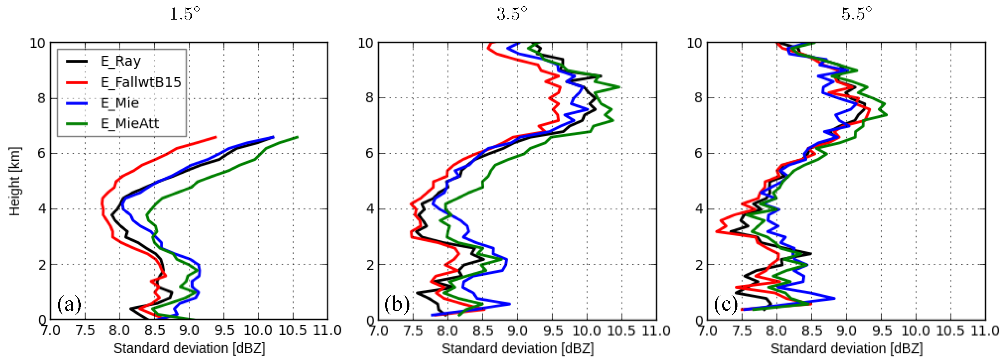
4.2.1. Standard Deviations of Estimated Observation Error

Figure 1 depicts the vertical profiles of the estimated standard deviations of the OE for reflectivity data ≥ 0 dBZ at elevations ${1.5}^{°}$, ${3.5}^{°}$, and ${5.5}^{°}$. First of all, Zeng et al. [23] showed, for the ICON-LAM-KENDA system, that the variations of standard deviations of the OE for reflectivity are primarily determined by the ground clutter effect for heights close to the surface and by the representation error due to unresolved scales and processes for heights up to 7 km, and aloft, the other error sources (e.g., from the microphysical scheme) might prevail. In the following, we concentrate more on differences caused by various types of the FE. For the elevation ${1.5}^{°}$ (see Figure 1a), the standard deviations of E_FallwtB15 are considerably smaller than E_Ray, especially at higher altitudes (respectively, longer distances). This is reasonable since the beam broadening effect becomes more pronounced with the increasing distance (note that $n_h\times n_v=1\times 5$ costs about 10% more computational time). The standard deviations of E_Ray are much smaller than those of E_Mie before, being slightly larger above 4 km. This could be attributed to considerably higher reflectivities produced by the Mie scattering scheme than the Rayleigh approximation at the brightband zone (the height of $0^{°}$ level is about 3 km) [10]. In the case of the Mie scattering scheme, above the 0 ${}^{°}$ C, the parameterization of starting melting temperature at $-10{}^{°}$ C might result in too-high Z, since graupel might not always be in wet growth mode in reality, and below 0 ${}^{°}$ C, the chosen EMA in combination with this “too-fast” microphysics melting parameterization leads to a too-narrow and peaky brightband. The too-fast melting is a common problem for all bulk schemes without prognostic water fractions for melting graupel and snow. Furthermore, from the point of view of data assimilation, another possible reason could be that the LETKF can better cope with the Rayleigh scattering scheme which may be less accurate but much more linear than the Mie scattering scheme. It is also noticed that due to the vertical localization, the standard deviations at the neighboring heights of the birghtband are also affected. By considering the attenuation in E_MieAtt, slightly smaller standard deviations than in E_Mie are obtained at altitudes lower than 3 km. However, for higher altitudes, reflectivities may become too low due to attenuation, leading to considerably larger errors. This may be attributed to the fact that the observed reflectivities have been already corrected for attenuation and, thus, the simulated reflectivities may be underestimated at higher altitudes compared to observations. On the other hand, this also indicates that the attenuation correction in observations is adequate. For ${3.5}^{°}$ (see Figure 1b), for altitudes lower than 7 km it also (almost) holds that the standard deviations of E_FallwtB15 (E_Mie) are smaller (larger) than those of E_Ray. Above 7 km, the standard deviations of E_FallwtB15 are smallest, followed by E_Mie and E_Ray. The standard deviations of E_MieAtt are slightly smaller than those of E_Mie till 4 km, and aloft, slightly larger. Overall, it is noticed that differences among experiments are smaller than for ${1.5}^{°}$, which is because, for the same height, the radar beams of higher elevations penetrate shorter distances than lower elevations, and thus they suffer less from omitting the beam broadening and attenuation effects. It can be seen for ${5.5}^{°}$ in Figure 1c that the differences among experiments further narrow.

As noted in Zeng et al. [23], Zeng et al. [50], the standard deviations of the estimated OE for reflectivity data ≥ 0 dBZ are prone to be underestimated (recall that $\mathbf{R}=10\times 10\times \mathbf{I}$$\left[{\mathrm{d}\mathrm{B}\mathrm{Z}}^2\right]$) since the same threshold value is set to both observations and backgrounds. To deal with this problem, we compute statistics again but based on reflectivity data ≥ 5 dBZ only, and results are shown in Figure 2. For all elevations, the standard deviations of the OE are much larger than in Figure 1 and vary more strongly with altitudes; however, the relative differences among experiments are comparable to those in Figure 1.

Figure 3 shows the vertical profiles of the estimated standard deviations of the OE for radial wind. For elevation ${1.5}^{°}$ (see Figure 3a), the standard deviations of all experiments are very close up to 2 km, and then the standard deviations of E_FallwtB15 become smaller than those of other experiments and these differences increase with height. Therefore, the FEs are insensitive to the options of the scattering schemes and the attenuation effect, and taking the beam broadening effect into account is important since the pulse volume becomes larger with increasing distance (the same for reflectivity). Furthermore, combining the beam broadening effect with the reflectivity weighting allows to account for the typically decreasing reflectivity with height accompanied by increasing wind speed on radial wind observations, which causes the radial wind to be systematically lower compared to estimates without considering both effects. For higher elevations (Figure 3b,c), the advantage of E_FallwtB15 over the other experiments is reduced because of shorter penetration distances and smaller pulse volumes (as mentioned above for reflectivity).

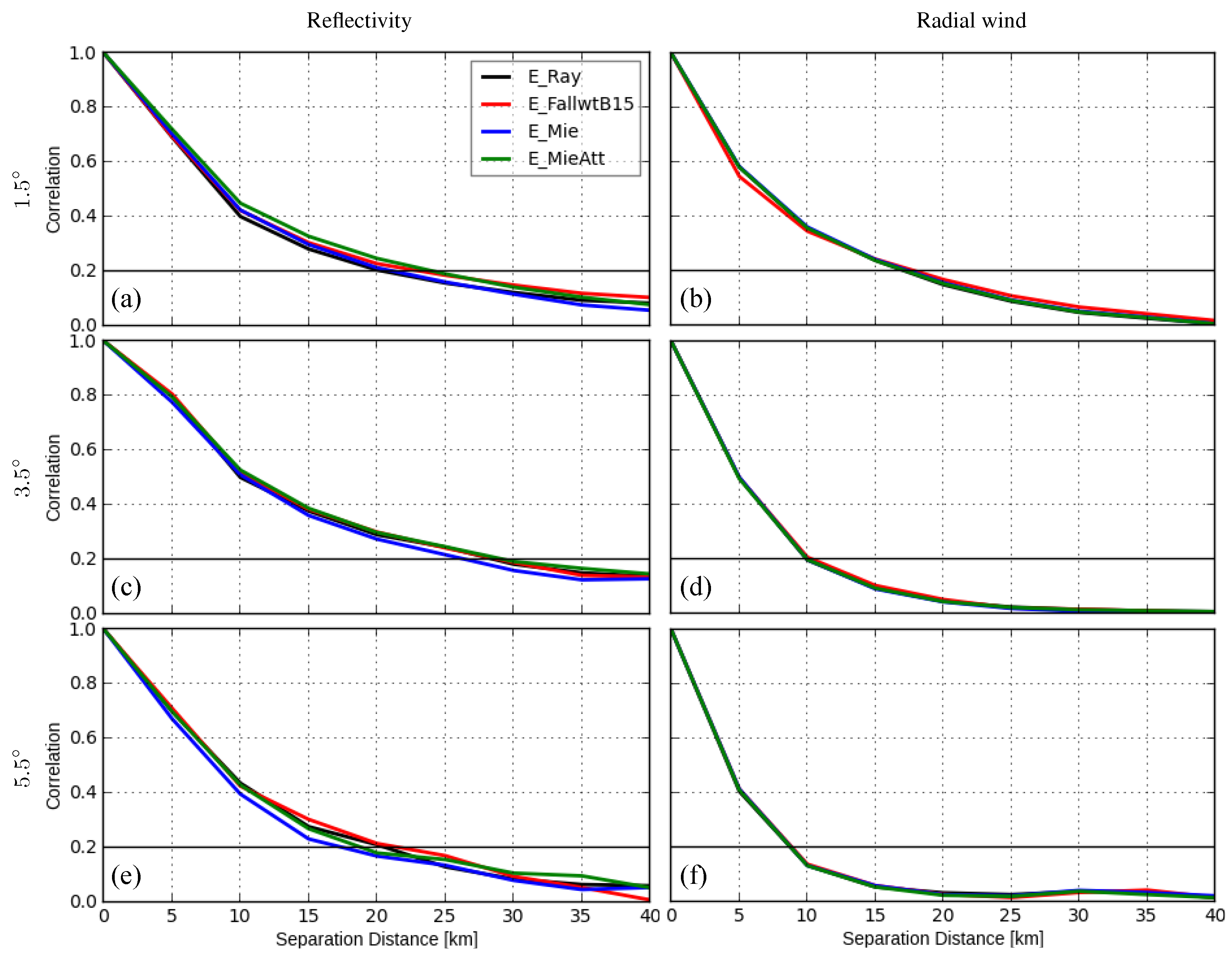
4.2.2. Correlation Length Scales of Estimated Observation Error

Figure 4 depicts the horizontal correlations of the OE for reflectivity data ≥ 5 dBZ for elevations ${1.5}^{°}$, ${3.5}^{°}$, and ${5.5}^{°}$ at heights of 3.0 and 6.0 km (correlations for reflectivity data ≥ 0 dBZ are not shown since they are very similar to Figure 4). For the elevation ${1.5}^{°}$ (see Figure 4a), the horizontal correlation length scales of E_Ray, E_FallwtB15, E_Mie, and E_MieAtt are about 22.5, 22.5, 25, and 30 km at the height of 3 km. Therefore, the application of the Mie scattering scheme slightly extends the length scales, which can be related to the overestimated reflectivities for the bright band. Moreover, accounting for the beam broadening does not shorten the length scales. Normally, a more advanced operator should reduce error correlation (and size) [25]; the neutral effects here may be due to the relatively coarse model grid, so that the same grid points may be used for simulating neighboring pulse volumes, which creates error correlations and compensates the advantage of a more complex operator. Finally, incorporating the attenuation effect considerably extends the length scales, which can be attributed to that the simulated reflectivities may be underestimated at longer distances compared to observations which were already corrected for attenuation. At the height of 6 km (see Figure 4b), the horizontal correlation length scale of E_Ray is about 40 km and the others are longer than 40 km, which are considerably longer than at 3 km. This is because radar beams are more influenced by errors (e.g., attenuation) when traveling longer distances for higher altitudes. For ${3.5}^{°}$ (see Figure 4c,d), the length scales are similar to those for ${1.5}^{°}$ at the height of 3 km, and at 6 km the length scales of E_FallwtB15, E_Mie, and E_MieAtt become shorter, probably due to shorter traveling distances for higher elevations. For ${5.5}^{°}$ (see Figure 4e,f), the length scales are generally comparable to those for ${3.5}^{°}$ but with some fluctuations (indicating that the numbers of samples may be not sufficient and results should be interpreted with caution).

Figure 5 depicts the horizontal correlations of the OE for radial wind. At the height of 3 km, the horizontal correlation length scales of E_Ray, E_FallwtB15, E_Mie, and E_MieAtt are about 30, 27.5, 30, and 30 km for the elevation ${1.5}^{°}$ (see Figure 5a), indicating slight positive effects of taking the beam broadening effect into account and neutral effects of choices of scattering schemes and attenuation. For ${3.5}^{°}$ and ${5.5}^{°}$ (see Figure 5c,e), the horizontal correlation length scales of all experiments are very similar, 20 km for ${3.5}^{°}$ and 10 km for ${5.5}^{°}$. Therefore, the higher the elevations are, the shorter the horizontal correlation length scales are (also seen in Zeng et al. [23]). At the height of 6 km, the horizontal correlation length scales of all experiments are also similar and longer than 40 km for ${1.5}^{°}$ (see Figure 5b), much longer than at the height of 3 km, and they also decrease with higher elevations. As stated in Zeng et al. [23], shorter length scales for higher elevations at the same height can be due to the fact that the radial wind is direction-sensitive and the lower elevations sense the horizontal component of the radial wind more than the vertical one, and the error correlations of the horizontal wind are usually associated with longer length scales than the vertical wind.

The along-beam correlations of the OE for both reflectivity data ≥ 5 dBZ and radial wind are given in Figure 6. For reflectivity, the along-beam correlation length scales of E_Ray, E_FallwtB15, E_Mie, and E_MieAtt are about 20, 22.5, 20, and 22.5 km for elevation ${1.5}^{°}$ (see Figure 6a). This indicates that accounting for beam broadening and attenuation effect both slightly extend the length scales, which is consistent with the horizontal correlation lengths, as shown in Figure 4. For ${3.5}^{°}$ (see Figure 6c), the slightly shorter length scale of E_Mie might be attributed to smaller errors at higher levels, as shown in Figure 2. For ${5.5}^{°}$ (see Figure 6e), the length scales of experiments are around 17.5 and 22.5 km (the numbers of samples may be not sufficient). For radial wind, the length scales of all experiments are very similar: about 17.5 km for ${1.5}^{°}$, 10 km for ${3.5}^{°}$ and 9 km for ${5.5}^{°}$, and, therefore, also shorter length scales for higher elevation, as for the horizontal correlations as shown in Figure 5.

5. Summary and Outlook

In the present work, we investigate the impacts on the observation error (OE) statistics due to different types of errors in the forward operator (FE) for both radar reflectivity and radial wind data, in the context of convective-scale data assimilation in a summertime. A series of sensitivity experiments were conducted based on the ICON-LAM-KENDA system of the DWD, with the radar forward operator EMVORADO, which belongs to the most comprehensive radar forward operators in the world. The investigated FEs are versatile, including errors caused by neglecting the terminal fall speed of hydrometeor, the reflectivity weighting, and the beam broadening and attenuation effects, as well as errors caused by different scattering schemes and formulations for melting particles. The OE statistics, including standard deviation, horizontal and along-beam correlations, are estimated by the Desroziers method.

For reflectivity, it is found that accounting for the beam broadening effect evidently reduces the standard deviations, especially at higher altitudes (respectively, longer distances). However, it does not shorten the horizontal or along-beam correlation length scales. This may be due to that the same model grid points are used for simulating neighboring pulse volumes and thus error correlations can be created. In comparison between the Rayleigh and the Mie schemes, the former one results in much smaller standard deviations for lower heights (up to 4 km), and aloft, slightly larger standard deviations. This is probably caused by the fact that the Mie scheme combined with the chosen EMA formulations produces too-high reflectivities at the brightband zone. Imposing the attenuation to the Mie scheme slightly reduces the standard deviations at lower altitudes; however, due to the fact that the radar reflectivity measurements were corrected for attenuation, it largely increases the standard deviations at higher altitudes and it also leads to longer correlation length scales. For radial wind, slight positive impacts of considering the beam broadening effect on standard deviations and neutral impacts on correlations are observed. For both reflectivity and radial wind, taking the terminal fall speed of hydrometeor and the reflectivity weighting into account does not make remarkable differences in the estimated OE statistics; it is possible that the other errors may dominate, e.g., inaccurate parameterizations for terminal fall speed or unresolvable updraft.

Radar data assimilation was recently adopted in the operational ICON-LAM-KENDA system, because of which the quality of short-term precipitation forecasts were greatly enhanced. The operational configurations of the EMVORADO are currently the Mie scheme with attenuation, taking the terminal fall speed of hydrometeor and the reflectivity weighting into account but neglecting the beam broadening effect. The results obtained in this work suggest that there is still a potential for improving those configurations. For instance, the beam broadening effect should be considered (only the vertical direction may be enough). Currently, we are testing the configurations for microphysical melting parameterization and the EMA formulations in the case of the Mie scattering scheme, and our aim is to find configurations that can appropriately reproduce the brightband. Given that reflectivity observations were corrected for attenuation, the attenuation should be neglected in simulation. Current results indicate that the attenuation correction in observations is sound, but more thorough tests may be needed to validate this, since as a goal we attempt to find appropriate configurations for the Mie scattering scheme without simulating attenuation effects.

Overall, the study shows the importance of quality of the radar forward operator and the impacts of the FE on the OE. It is recommendable to account for the beam broadening effect, and the brightband issue is still challenging; more efforts should especially be devoted to improving the simulation of melting particles. It should be noted that inaccurate parameterizations can also contribute to the FE, which was not shown in this study but is worth exploring. To the end, the improved configurations may allow smaller variances in the OE covariance matrix and, thus, better adoption of information embedded in observations by the model. In the next step, the impacts of improved configurations on the short-term forecasts will be examined. In addition, the statistics presented here can also serve as a guideline for constructing the full OE covariance matrix for radar data in the future. Finally, it is worth noting that although this study has been conducted with the EMVORADO in the ICON-LAM-KENDA system, its results can be also useful for the other radar data assimilation communities while setting configurations for their operators, since some of the problems are quite general in the radar forward operator.

References

1. Simonin, D.; Ballard, S.; Li, Z. Doppler radar radial wind assimilation using an hourly cycling 3D-Var with a 1.5 km resolution version of the Met Office Unified Model for nowcasting. Q. J. R. Meteorol. Soc. 2014, 140, 2298–2314. [Google Scholar] [CrossRef]
2. Wattrelot, E.; Caumont, O.; Mahfouf, J. Operational implementation of the 1D+3D-Var assimilation method of radar reflectivity data in the AROME model. Mon. Weather Rev. 2014, 142, 1852–1873. [Google Scholar] [CrossRef] [Green Version]
3. Schraff, C.; Reich, H.; Rhodin, A.; Schomburg, A.; Stephan, K.; Periáñez, A.; Potthast, R. Kilometre-Scale Ensemble Data Assimilation for the COSMO Model (KENDA). Q. J. R. Meteorol. Soc. 2016, 142, 1453–1472. [Google Scholar] [CrossRef]
4. Gustafsson, N.; Janjić, T.; Schraff, C.; Leuenberger, D.; Weissman, M.; Reich, H.; Brousseau, P.; Montmerle, T.; Wattrelot, E.; Bucanek, A.; et al. Survey of data assimilation methods for convective-scale numerical weather prediction at operational centres. Q. J. R. Meteorol. Soc. 2018, 144, 1218–1256. [Google Scholar] [CrossRef] [Green Version]
5. Zängl, G.; Reinert, D.; Rïpodas, P.; Baldauf, M. The ICON (ICOsahedral Non-hydrostatic) modelling framework of DWD and MPI-M: Description of the non-hydrostatic dynamical core. Q. J. R. Meteorol. Soc. 2015, 141, 563–579. [Google Scholar] [CrossRef]
6. Bick, T.; Simmer, C.; Trömel, S.; Wapler, K.; Stephan, K.; Blahak, U.; Zeng, Y.; Potthast, R. Assimilation of 3D-Radar Reflectivities with an Ensemble Kalman Filter on the Convective Scale. Q. J. R. Meteorol. Soc. 2016, 142, 1490–1504. [Google Scholar] [CrossRef] [Green Version]
7. Hunt, B.R.; Kostelich, E.J.; Szunyogh, I. Efficient data assimilation for Spatiotemporal Chaos: A Local Ensemble Transform Kalman Filter. Phys. Nonlinear Phenom. 2007, 230, 112–126. [Google Scholar] [CrossRef] [Green Version]
8. Zeng, Y. Efficient Radar Forward Operator for Operational Data Assimilation within the COSMO-Model. Ph.D. Dissertation, Karlsruhe Insititute of Technology, Karlsruhe, Germany, 2013. [Google Scholar]
9. Zeng, Y.; Blahak, U.; Neuper, M.; Jerger, D. Radar Beam Tracing Methods Based on Atmospheric Refractive Index. J. Atmos. Ocean. Technol. 2014, 31, 2650–2670. [Google Scholar] [CrossRef]
10. Zeng, Y.; Blahak, U.; Jerger, D. An efficient modular volume-scanning radar forward operator for NWP models: Description and coupling to the COSMO model. Q. J. R. Meteorol. Soc. 2016, 142, 3234–3256. [Google Scholar] [CrossRef]
11. Blahak, U.; RADAR_MIE_LM and RADAR_MIELIB – Calculation of Radar Reflectivity from Model Output. COSMO Technical Report No. 28, Consortium for Small Scale Modeling. 2016. Available online: http://www.cosmo-model.org/content/model/documentation/techReports/cosmo/docs/techReport28.pdf (accessed on 20 June 2022).
12. Blahak, U.; de Lozar, A. EMVORADO—Efficient Modular VOlume scan RADar Operator. A User’s Guide; Deutscher Wetterdienst: Offenbach, Germany, 2021. [Google Scholar]
13. Trömel, S.; Simmer, C.; Blahak, U.; Blanke, A.; Ewald, F.; Frech, M.; Gergely, M.; Hagen, M.; Hörnig, S.; Janjic, T.; et al. Overview: Fusion of Radar Polarimetry and Numerical Atmospheric Modelling Towards an Improved Understanding of Cloud and Precipitation Processes. Atmos. Chem. Phys. Discuss. 2021, 2021, 1–36. [Google Scholar] [CrossRef]
14. Gastaldo, T.; Poli, V.; Marsigli, C.; Cesari, D.; Alberoni, P.P.; Paccagnella, T. Assimilation of radar reflectivity volumes in a pre-operational framework. Q. J. R. Meteorol. Soc. 2021, 147, 1031–1054. [Google Scholar] [CrossRef]
15. Janjic, T.; Bormann, N.; Bocquet, M.; Carton, J.A.; Cohn, S.E.; Dance, S.L.; Losa, S.N.; Nichols, N.K.; Potthast, R.; Waller, J.A.; et al. On the representation error in data assimilation. Q. J. R. Meteorol. Soc. 2018, 144, 1257–1278. [Google Scholar] [CrossRef]
16. Hollingsworth, A.; Lonnberg, P. The statistical structure of short-range forecast errors as determined from radiosonde data. Part 1: The wind field. Tellus 1986, 38, 111–136. [Google Scholar] [CrossRef] [Green Version]
17. Desroziers, G.; Berre, L.; Chapnik, B.; Poli, P. Diagnosis of observation, background and analysis-error statistics in observation space. Q. J. R. Meteorol. Soc. 2005, 131, 3385–3396. [Google Scholar] [CrossRef]
18. Wattrelot, E.; Montmerle, T.; Guerrero, C. Evolution of the assimilation of radar data in the AROME model at Météo-France. In Proceedings of the Seventh European Conference on Radar in Meteorology and Hydrology, Toulouse, France, 24–29 June 2012. [Google Scholar]
19. Simonin, D.; Waller, J.A.; Ballard, S.P.; Dance, S.L.; Nichols, N.K. A pragmatic strategy for implementing spatially correlated observation errors in an operational system: An application to Doppler radial winds. Q. J. R. Meteorol. Soc. 2019, 145, 2772–2790. [Google Scholar] [CrossRef]
20. Fujita, T.; Seko, H.; Kawabata, T.; Ikuta, Y.; Sawada, K.; Hotta, D.; Kunii, M. Variational Data Assimilation with Spatial and Temporal Observation Error Correlations of Doppler Radar Radial Winds. In Proceedings of the Working Group on Numerical Experimentation, Report No. 50.WCRP Report No.12/2020, Online, 2–5 November 2020. [Google Scholar]
21. Doviak, R.J.; Zrnic, D.S. Doppler Radar and Weather Observations; Academic Press, Inc.: San Diego, CA, USA, 1993; Volume 2. [Google Scholar]
22. Xue, M.; Jung, Y.; Zhang, G. Error modeling of simulated reflectivity observations for ensemble Kalman filter assimilation of convective storms. Geophys. Res. Lett. 2007, 148, L10802. [Google Scholar] [CrossRef] [Green Version]
23. Zeng, Y.; Janjic, T.; Feng, Y.; Blahak, U.; de Lozar, A.; Bauernschubert, E.; Stephan, K.; Min, J. Interpreting estimated Observation Error Statistics of Weather Radar Measurements using the ICON-LAM-KENDA System. Atmos. Meas. Tech. 2021, 14, 5735–5756. [Google Scholar] [CrossRef]
24. Jung, Y.; Xue, M.; Zhang, G. Simulations of Polarimetric Radar Signatures of a Supercell Storm Using a Two-Moment Bulk Microphysics Scheme. J. Appl. Meteorol. Clim. 2010, 49, 146–163. [Google Scholar] [CrossRef]
25. Waller, J.A.; Simonin, D.; Dance, S.L.; Nichols, N.K.; Ballard, S.P. Diagnosing Observation Error Correlations for Doppler Radar Radial Winds in the Met Office UKV Model Using Observation-Minus-Background and Observation-Minus-Analysis Statistics. Mon. Weather Rev. 2016, 144, 3533–3551. [Google Scholar] [CrossRef]
26. Waller, J.A.; Dance, S.L.; Nichols, N.K. Theoretical insight into diagnosing observation error correlations using observation-minus-background and observation-minus-analysis statistics. Q. J. R. Meteorol. Soc. 2016, 142, 418–431. [Google Scholar] [CrossRef] [Green Version]
27. Waller, J.A.; Bauernschubert, E.; Dance, S.L.; Nichols, N.K.; Potthast, R.; Simonin, D. Observation Error Statistics for Doppler Radar Radial Wind Superobservations Assimilated into the DWD COSMO-KENDA System. Mon. Weather Rev. 2019, 147, 3351–3364. [Google Scholar] [CrossRef] [Green Version]
28. Lin, Y.; Farley, R.D.; Orville, H.D. Bulk parameterization of the snow field in a cloud model. J. Clim. Appl. Meteorol. 1983, 22, 1065–1092. [Google Scholar] [CrossRef] [Green Version]
29. Reinhardt, T.; Seifert, A. A three-category ice scheme for LMK. COSMO News Lett. 2006, 6, 115–120. [Google Scholar]
30. Seifert, A.; Beheng, K.D. A two-moment cloud microphysics parameterization for mixed-phase clouds. Part I: Model description. Meteorol. Atmos. Phys. 2006, 92, 45–66. [Google Scholar] [CrossRef]
31. Raschendorfer, M. The New Turbulence Parametrization of LM; COSMO-Newsletter; Consortium for Smallscale Modeling: Offenbach, Germany, 2001; Volume 1. [Google Scholar]
32. Tiedtke, M. A comprehensive mass flux scheme for cumulus parameterization in large-scale models. Mon. Weather Rev. 1989, 117, 1779–1799. [Google Scholar] [CrossRef] [Green Version]
33. Werner, M. A New Radar Data Post-Processing Quality Control Workflow for the DWD Weather Radar Network. In Proceedings of the Eighth European Conference on Radar in Meteorology and Hydrology, Garmisch-Partenkirchen, Germany, 1–5 September 2014. [Google Scholar]
34. Stephan, K.; Klink, S.; Schraff, C. Assimilation of radar-derived rain rates into convective-scale model COSMO-DE at DWD. Q. J. R. Meteorol. Soc. 2008, 134, 1315–1326. [Google Scholar] [CrossRef]
35. Press, W.H.; Teukolsky, S.A.; Vetterling, W.T.; Flannery, B.P. Numerical Recipes in Fortran 77; Cambridge University Press: Cambridge, UK, 1993. [Google Scholar]
36. Blahak, U. An approximation to the effective beam weighting function for scanning meteorological radars with axissymmetric antenna pattern. J. Atmos. Ocean. Technol. 2008, 25, 1182–1196. [Google Scholar] [CrossRef]
37. Ray, P.S. Broadband complex refractive indices of ice and water. Appl. Opt. 1972, 11, 1836–1844. [Google Scholar] [CrossRef]
38. Liebe, H.J.; Hufford, G.A.; Manabe, T. A model for the complex permittivity of water at frequencies below 1THz. Int. J. Infrared Millim. Waves 1991, 12, 659–675. [Google Scholar] [CrossRef]
39. Warren, S.G. Optical constants of ice from the ultraviolet to the microwave. Appl. Opt. 1984, 23, 1029–1078. [Google Scholar] [CrossRef]
40. Mätzler, C. Microwave properties of ice and snow. Sol. Syst. Ices Astrophys. Space Sci. Libr. 1998, 227, 241–257. [Google Scholar]
41. Wolfensberger, D.; Berne, A. From model to radar variables: A new forward polarimetricradar operator for COSMO. Atmos. Meas. Tech. 2018, 11, 3883–3916. [Google Scholar] [CrossRef] [Green Version]
42. Maxwell-Garnett, J.C. Colours in metal glasses and in metallic films. Proc. R. Soc. Lond. 1904, A203, 385–420. [Google Scholar]
43. Bruggemann, D.A.G. Brechung verschiender physikalischer Konstanten von heteogenes Substanzen I. Dielektrizitätskonstanten und Leitfähigkeiten der Misachkörper aus isotropen Substanzen. Ann. Phys. 1935, 416, 636–664. [Google Scholar] [CrossRef]
44. Oguchi, T. Electromagnetic wave propagation and scattering in rain and other hydrometeors. Proc. IEEE 1983, 71, 1029–1078. [Google Scholar] [CrossRef]
45. Batten, L.; Bohren, C. Radar backscattering by melting snowflakes. J. Appl. Meteorol. 1982, 21, 1937–1938. [Google Scholar] [CrossRef] [Green Version]
46. Lange, H.; Janjić, T. Assimilation of Mode-S EHS Aircraft Observations in COSMO-KENDA. Mon. Weather Rev. 2016, 144, 1697–1711. [Google Scholar] [CrossRef]
47. Zeng, Y.; Janjić, T.; de Lozar, A.; Blahak, U.; Reich, H.; Keil, C.; Seifert, A. Representation of model error in convective-scale data assimilation: Additive noise, relaxation methods and combinations. J. Adv. Model. Earth Syst. 2018, 10, 2889–2911. [Google Scholar] [CrossRef] [Green Version]
48. Feng, Y.; Janjić, T.; Zeng, Y.; Seifert, A.; Min, J. Representing microphysical uncertainty in convective-scale data assimilation using additive noise. J. Adv. Model. Earth Syst. 2021, 13, e2021MS002606. [Google Scholar] [CrossRef]
49. Aksoy, A.; Dowell, D.C.; Snyder, C. A multiscale comparative assessment of the ensemble Kalman filter for assimilation of radar observations. Part I: Storm-scale analyses. Mon. Weather Rev. 2009, 137, 1805–1824. [Google Scholar] [CrossRef] [Green Version]
50. Zeng, Y.; Janjic, T.; de Lozar, A.; Welzbacher, C.A.; Blahak, U.; Seifert, A. Assimilating radar radial wind and reflectivity data in an idealized setup of the COSMO-KENDA system. Atmos. Res. 2021, 249, 105282. [Google Scholar] [CrossRef]
51. Anderson, J.L. Spatially and temporally varing adaptive covariance inflation for ensemble filters. Tellus 2009, 61A, 72–83. [Google Scholar] [CrossRef]
52. Zhang, F.; Snyder, C.; Sun, J. Impacts of initial estimate and observation availability on convective-scale data assimilation with an ensemble Kalman filter. Mon. Weather Rev. 2004, 132, 1238–1253. [Google Scholar] [CrossRef]
53. Janjic, T.; Zeng, Y. Weakly constrained LETKF for estimation of hydrometeor variables in convective-scale data assimilation. Geophys. Res. Lett. 2021, 48, e2021GL094962. [Google Scholar] [CrossRef]
54. Waller, J.A.; Ballard, S.P.; Dance, S.L.; Kelly, G.; Nichols, N.K.; Simonin, D. Diagnosing horizontal and inter-channelobservation error correlations for SEVIRI observations using observation-minus-background and observation-minus-analysis statistics. Remote Sens. 2016, 8, 581. [Google Scholar] [CrossRef] [Green Version]
55. Weissmann, M.; Göber, M.; Hohenegger, C.; Janjić, T.; Keller, J.; Ohlwein, C.; Seifert, A.; Trömel, S.; Ulbrich, T.; Wapler, K.; et al. Initial phase of the Hans-Ertel Centre for Weather Research - A virtual centre at the interface of basic and applied weather and climate research. Meteorol. Z. 2014, 23, 193–208. [Google Scholar] [CrossRef]
56. Simmer, C.; Adrian, G.; Jones, S.; Wirth, V.; Göber, M.; Hohenegger, C.; Janjić, T.; Keller, J.; Ohlwein, C.; Seifert, A.; et al. HErZ – The German Hans-Ertel Centre for Weather Research. Bull. Am. Meteorol. Soc. 2016, 97, 1057–1068. [Google Scholar] [CrossRef]
Figure 1. Vertical profiles of the estimated standard deviations of the OE for reflectivity data ≥ 0 dBZ at elevations 1.5 ° (a), 3.5 ° (b), and 5.5 ° (c). For each elevation, the samples are binned every 200 m in the vertical. It is possible for each elevation that samples are not available for some heights.
Remotesensing 14 03685 g001
Figure 2. The same as Figure 1, but for reflectivity data ≥ 5 dBZ (ac).
Remotesensing 14 03685 g002
Figure 3. The same as Figure 1, but for radial wind (ac).
Remotesensing 14 03685 g003
Figure 4. The estimated horizontal correlations of the OE for reflectivity data ≥ 5 dBZ for elevations 1.5 ° , 3.5 ° , and 5.5 ° at heights of 3.0 (a,c,e) and 6.0 km (b,d,f). For each elevation, the samples are binned every 5 km in the separation distance.
Remotesensing 14 03685 g004
Figure 5. (af), The same as Figure 4, but for radial wind. Note that the black line is strongly overlapped with blue and green lines in panel (a).
Remotesensing 14 03685 g005
Figure 6. Along-beam correlation length scales of Desroziers statistics for reflectivity ≥ 5 dBZ and radial wind for elevations 1.5 ° (a,b), 3.5 ° (c,d), and 5.5 ° (e,f). Correlations are expressed as a function of the separation distance along the beam, and the samples are binned every 5 km in the (radial) separation distance.
Remotesensing 14 03685 g006