Article

Deep Learning-Based Water Quality Retrieval in an Impounded Lake Using Landsat 8 Imagery: An Application in Dongping Lake

1
College of Water Sciences, Beijing Normal University, Xinjiekouwai Street 19, Haidian, Beijing 100875, China
2
Environment Research Institute, Shandong University, Jinan 250100, China
*
Author to whom correspondence should be addressed.
Remote Sens. 2022, 14(18), 4505; https://doi.org/10.3390/rs14184505
Submission received: 1 August 2022 / Revised: 29 August 2022 / Accepted: 1 September 2022 / Published: 9 September 2022

Abstract

:
Attempts have been made to incorporate remote sensing techniques and in situ observations for enhanced water quality assessments. Estimations of nonoptical indicators sensitive to water environment changes, however, have not been fully studied, mainly due to complex nonlinear relationships between the observed values and surface reflectance. In this study, we applied a novel deep learning approach driven by a range of spectral properties to retrieve 6-year changes in water quality variables, i.e., Chl-a, BOD, TN, CODMn, NH3-N, and TP, on a monthly basis between 2013 and 2018 at Dongping Lake, an impounded lake located in the Yellow River in China. Band arithmetic was used to compute 26 predictors from Landsat 8 OLI imagery for model inputs. The results showed generally strong agreement between in situ and ConvLSTM-derived lake variables, generating R2 of 0.92, 0.88, 0.84, 0.80, 0.83, and 0.77 for TN, NH3-N, CODMn, Chl-a, TP, and BOD, which suggest good performance of the developed model. We then used statistical analysis to identify the spatial and temporal heterogeneity. The framework established in this study has applications in effective water quality monitoring and serves as an alarming tool for water-environment management in the complex inland lake waters.

Graphical Abstract

1. Introduction

Documentation related to water quality in different regions and water bodies combines to yield a complex water issue map of the world. Living in close proximity to endangered water bodies increases the risk of exposure to public health threats as well as a decline in residential property. On the other hand, the growing population and excess nutrient and chemical loads from anthropological activities have increased freshwater ecosystem stresses [1,2,3,4,5]. Further aggravated by uneven distribution and lack of water, the impaired water quality in China has posed an enormous threat to society and freshwater ecosystems. To address the problem, the Chinese government has come forward the with South–North Water Diversion Project (SNWDP), drawing water from the rainy low latitudes to relatively dry and less rainy high latitudes. Since 2002, the eastern route of the SNWDP (SNWDP-ER) has diverted enormous quantities of water and significantly impacted the water quality in its receiving areas [6,7]. Effective water quality monitoring is identified as the key to protecting and restoring the integrity of ecosystems, achieving sustainability in water quality, benefiting human well-being, and boosting socioeconomic development [8,9,10,11,12]. Traditional monitoring techniques, broadly defined as in situ observations, however, are considered too costly for local environmental uses for extracting the varying spatiotemporal features. This inevitably poses a challenge to addressing aquatic issues and public health concerns. Therefore, it has gradually evolved as a supplement and validation of other water quality monitoring methods.
For this reason, it is important to monitor the surface water in a more flexible and appropriate way. To date, numerous studies have explored the potential and utility of remote sensing techniques in bettering our knowledge of environmental characteristics on varying temporal and spatial scales. Satellites equipped with various optical and thermal sensors are more advantageous than in situ measurements in providing the ever-increasing stream of geospatial data covering large areas with high resolution, as well as being more economical [2,9,13,14,15,16,17,18,19,20]. Low- or medium-resolution hyperspectral sensors, such as MERIS, MODIS, and SeaWiFS, have been adopted by researchers for many years for water quality assessment, and research conducted in large rivers and lakes, estuaries, and coastal areas or on a regional scale has demonstrated applicability in satellite-based water quality estimations [15,21,22,23,24,25,26]. Nevertheless, they are not very suitable for monitoring small lakes or rivers due to limited spatial information. Much literature has revealed the efficacy of multispectral Landsat sensors, including TM (Thematic Mapper), MSS (Multispectral Scanner), ETM (Enhanced Thematic Mapper), and OLI (Operational Land Imager), for the retrieval of commonly measured water quality variables. Being quite accessible and with appropriate temporal frequency and spatial resolution, the Landsat satellite-based datasets enable monthly monitoring in smaller areas of inland water bodies and provide key information for local policymakers and water-environment, managers as well as researchers. Water constituents, such as chlorophyll, Secchi disk depth (SDD), total suspended matter (TSM), colored dissolved organic matter (CDOM), and others, defined as optically active variables, have been widely studied by many researchers [27,28,29,30,31,32,33,34,35,36,37]. However, several other important indices are nonoptically active, such as chemical oxygen demand (COD), biological oxygen demand (BOD), total nitrogen (TN), permanganate of chemical oxygen demand (CODMn), ammonia (NH3-N), and total phosphorus (TP), and have not been well explored and remain a challenging aspect of comprehensive water quality evaluation. Furthermore, most previous studies that estimated the water quality condition in the impounded lakes in China have rarely focused on specific seasons or were dependent on point scales with limited laboratory analytic data. This highlights the necessity to effectively estimate both optically active and inactive variables and examine their spatiotemporal patterns, thus facilitating a bigger picture of water quality conditions by aquatic environment managers.
Different approaches are introduced in water quality remote sensing investigations to enhance our knowledge of the water system. Typical methodology to interpret and evaluate the concentrations of different variables has evolved from empirical regression methods including simple linear regression and nonlinear multiple regression to principal component analysis (PCA) and neural networks [20,28,32,38]. A number of these investigations have also utilized band math algorithms to select both correlated single bands and band ratios for mapping the spatial distribution of indicators [30,39]. Nevertheless, some conventional regression models may not be optimal, especially when there are complex nonlinear relationships between water system behaviors and environmental factors. In recent years, rather than amending classical approaches, leveraging big-data tools and technologies in the water quality sector has become a consensus. Although some machine learning-based evaluations have shown promising results in tackling the low accuracy in time series using simple empirical models, it remains a challenge to thoroughly understand the complex bidirectional interactions between water constituents and solar radiation in temporal and spatial contexts [10,13,40,41,42]. Deep learning techniques provide an opportunity to learn the more sophisticated statistical characteristics, yet have sometimes forcibly separated the spatial or temporal correlation characteristics [15,43,44,45]. Recent studies looking into the abilities in the data-driven estimation of ecological factors, such as soil moisture, have found the novel artificial intelligence approach (AI) of convolutional long short-term memory (ConvLSTM) model dramatically outperformed classical sequence modeling methods in capturing the spatiotemporal correlations of the satellite image inputs. However, attempts at applying the ConvLSTM algorithm to water quality retrieval are still rare, which underlines the need for special attention applying to the challenging water quality modeling.
The fact that water quality issues are associated with plural environmental and anthropogenic factors has made the accurate prediction of water quality constituents particularly difficult. In this study, we developed a novel deep learning-based regression model of ConvLSTM, designed specifically for both optically active and inactive water quality modeling. By incorporating the Landsat 8 OLI imagery into the developed model, we attempt to propose a highly accurate method for inland lake monitoring that is potentially powerful in mapping the nonlinear spatial–spectral information at relatively high spatial resolution. In addition to retrieving the concentration of water quality parameters, detection of variations from different temporal and spatial perspectives for these water quality indicators were performed to provide better knowledge and insights into the contrasting spatiotemporal patterns in an impounded lake. Accordingly, the aims of the study were to: (1) investigate the utility of the ConvLSTM-based deep learning method with processed Landsat 8 OLI remotely sensed imagery, (2) to evaluate the accuracy of the ConvLSTM-derived concentration of both optically active and inactive water quality variables, and (3) to map the distribution for the range of water quality indicators and identify the dynamics in time and space. A schematic flowchart of the developed framework for water quality retrieval and spatiotemporal variation assessment using remote sensing and deep learning techniques is presented in Figure 1.

2. Materials and Methods
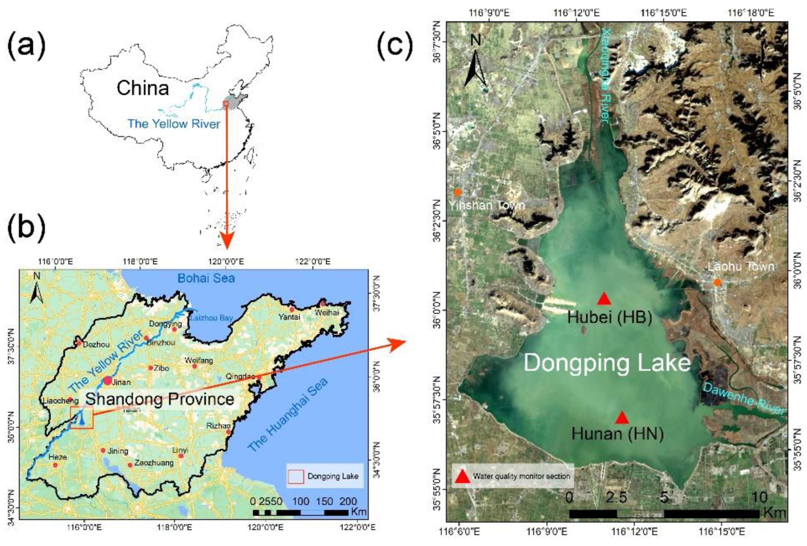
2.1. Study Area

Dongping Lake (DPL) is a typical inland freshwater lake, located in Dongping County, Tai’an City, western Shandong Province in China (116°00′~116°20′E, 35°50′–36°20′N) (Figure 2). Mainly recharged by the Liuchanghe River in the south, the lake water flows from south to north into the Yellow River in the west of Shandong (Figure 2b,c). The lake encompasses an area of 627 km2, stores 3980 million m3 of water, and has an average multiyear water depth of 1–2 m. This region has a warm temperate monsoon climate with an annual average temperature of 13.6 °C. Unevenly distributed over the year, most of the precipitation in this area happens in the flood season (from June to September), and the annual average rainfall is 663 mm [46,47,48].
Officially implemented on 15 November 2013, the SNWDP-ER draws water from the Yangzhou Jiangdu Water Conservancy Hub in Jiangsu Province, transfers water from a series of impounded lakes from south to north, and finally diverts water from Baliwan Pumping Station into Dongping Lake, which supplies water to the north of the Yellow River and Jiao Dong region. As the last level of water transfer and storage lake in the SNWDP-ER, the water quality of DPL is directly related to the water supply safety of the northern receiving area of the Yellow River and could have a great impact on the local ecology and economy. The months in which water transfer occurred in DPL during the study period are listed in Table 1 [7,49,50]. According to the files issued by the state council, the comprehensive water quality of DPL should be consistently up to the Class III standard according to the Chinese Environmental Quality Standard for Surface Water (GB3838-2002) before the water transfer. Nevertheless, the DPL has experienced several outbreaks of algae that have brought public awareness of the risk of eutrophication and water pollution issues [7,46,47].

2.2. Data

2.2.1. Satellite Data

Launched on 11 February 2013 by the National Aeronautics and Space Administration (NASA), Landsat 8 OLI is one of the most commonly used satellites for water quality monitoring. Being a sun-synchronous spaceborne satellite, the OLI sensor has an orbital altitude of 705 km and an orbital inclination of 98.2° with a revisit interval of 16 days. It has a spatial resolution of 15–30–100 meters with each image covering 170 km in width. Apart from all of the bands in the Enhanced Thematic Mapper Plus (ETM+) sensor mounted on Landsat 7, particular spectral properties were added to the Landsat 8 OLI sensor. There are two more bands in the OLI sensor, i.e., the blue band (band 1; 0.433–0.453 μm), mainly used for coastal zone observations, and the short-wave infrared band (band 9; 1.360–1.390 μm), representing a strong absorption feature for water vapor that can be used for cloud detection. As a result, there are a total of nine bands for OLI sensors with a wavelength ranging from 430 to 1380 nm. The Landsat 8 Operational Land Imager (OLI) datasets for the period between April 2013 to December 2018 were obtained via the publicly free website (http://glovis.usgs.gov/ (accessed on 24 June 2022)) supported by the US Geological Survey (USGS). In this study, a total of 69 scenes of OLI imagery with a cloud cover of less than 10% were gathered.

2.2.2. In Situ Water Quality Observation Data
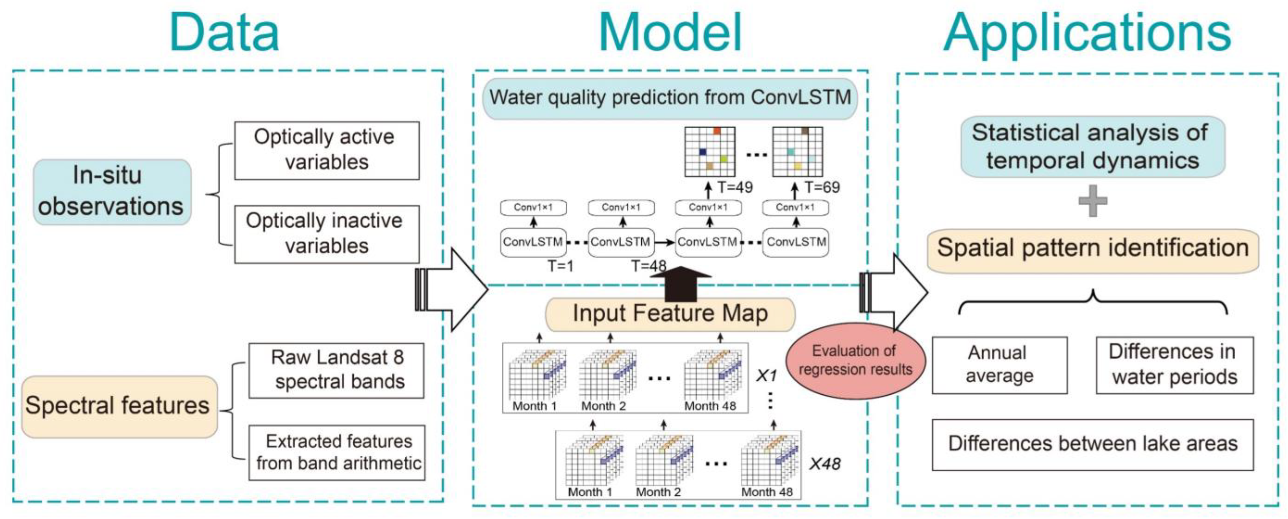
A system of physicochemical indices according to the GB3838-2002 standard, including Chl-a, BOD, TN, CODMn, NH3-N, and TP, were obtained from the local government of Shandong Province [51,52]. The two national cross sections within the lake, i.e., Hunan (HN) and Hubei (HB) sections, provided in situ observations from April 2013 to December 2018 in the upper and middle reaches of the lake (Figure 2c). The measurements in accordance with the passing dates of the satellite were paired to the corresponding remotely sensed imagery, thus generating a total of 138 pairs of monthly datasets. The major over-standard pollutants exceeding the range of Class III surface water specified by the GB3838-2002 standard of DPL were found to be TN and TP for both national cross sections.

2.3. Method

2.3.1. Preparation and Processing of the Satellite Imagery

Solar radiation receives aerosols, mists, and features during transmission, resulting in the sensor’s raw image containing not only information reflected from the surface of the object but also some false information. Therefore, several preprocessing steps were applied for all Landsat 8 images before being used as inputs for the water quality model. As the Landsat 8 L1T images have been geometrically corrected by DEM, the overall preprocessing workflow began with radiometric calibration that converted the raw digital numbers (DNs) values for each band to units of top-of-atmosphere (TOA) reflectance with common reference values. With radiometric calibration, interference induced by the atmosphere and the sensor itself can be diminished as well. The calibrated data were then atmospherically corrected to allow the conversion from spectral radiance to water–surface reflectance. A simplified atmospheric radiative transfer model is used here for atmospheric correction, which takes into account the effect of atmospheric scattering, and also the effect of solar altitude angle in the transmission of surface information [29]:
ρ tg = L i L min E 0 cos θ 0 d
where ρ tg is the surface reflectance of the target and L ds and L ts denote the radiant brightness value and the dark object radiance at the sensor, respectively. E 0 d is the solar irradiance at the top of the atmosphere, and θ 0 is the solar zenith angle. The atmospheric correction is processed in ENVI 5.3 platform using the FLAASH methodology, which builds its physics-based algorithms based on the MODTRAN4 radiative transfer code. By allowing a range of choice of atmospheric models and accurately compensating for atmospheric effects, the procedure has facilitated remote sensing water quality monitoring in many applications.
The processed satellite products contained well-corrected surface reflectance values for the nine bands of Landsat 8 OLI imagery. The remotely sensed images were further masked to extract the water-only contents out of the undesired area. Representative square sampling areas of 90 × 90 m (3 × 3 pixel) were created, centered on the pixel where the two cross sections are located. These sampling areas were manually demarcated to diminish adjacency effects. Then, the value of each pixel within the small sets of samples was averaged for each band as input spectral data for the modeling process. The resulting Landsat imagery database generated a total of 69 scenes for Dongping Lake from April 2013 to 18 December 2018.

2.3.2. Feature Extraction

Band ratio/arithmetic, a semiempirical method for the retrieval of water quality parameters, has been extensively researched and applied in remotely sensed monitoring of inland water bodies. demonstrating promising results [53,54,55,56,57,58,59]. By establishing a mathematical ratio consisting of the reflectance of two or more spectral bands, the band arithmetic approach provides a number of new variables that would benefit the regression analysis of water constituents. The simple form of this method can be described as follows:
p ^ = α R 1 R 2 β + γ
where p ^ is the estimated water quality variable, R i is the reflectance of Bandi, and α, β, and γ are the coefficients from the regression model. To better exploit the complex interaction between the measurements and the spectral signals from the sensors, as well as to extract extra biophysical properties for optically active and inactive constituents, a list of band ratios is computed from the processed OLI dataset. As displayed in Table 2, this produces a total of 26 predictor features representing the spectral reflectance features of the given sampling area, which are later used as the inputs of the estimation model.

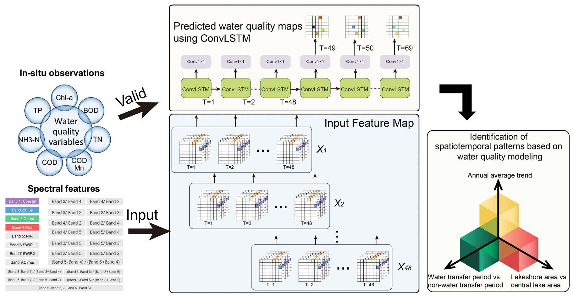
2.3.3. ConvLSTM-Derived Water Quality Estimation

The convolutional long short-term memory (ConvLSTM) model, introduced by [41], was proposed as an extension of the fully connected LSTM (FC-LSTM) model and was originally applied to address the spatiotemporal sequence forecasting problem in precipitation nowcasting. By stacking multiple recurrent ConvLSTM layers, which are similar to those layers in LSTM, yet exchanging the internal matrix multiplications, with convolution operations, this algorithm includes convolutional structures in both the input-to-state and state-to-state transitions. As a key constituent of the model, the three-dimensional (3D) ConvLSTM layer height, weight, and depth make use of the weight sharing to reduce the number of parameters and their redundancy in the same way as in a convolutional neural network (CNN). The way that a ConvLSTM network treats input data as a sequence enables the mode to deal with time-series data as a recurrent neural network. As a result, both temporal and spatial information that contain complex and deep features can be encoded, thus facilitating more general spatiotemporal sequence modeling. Moreover, the adoption of the nonlinear ReLU activation function as part of the optimization strategies is also reported to promote modeling performance. The key to overcoming spatial data redundancy is related to the unique design of ConvLSTM, where the input X t , memory cell outputs C t , hidden states H t , and gates i t , f t , o t of the network are 3D tensors, with the last two dimensions representing spatial dimensions (rows and columns). The controlling equations of the model are shown below, where ‘ ’ denotes the convolution operator and ‘ ’ denotes the Hadamard product.
i t = σ W x i X t + W h i H t 1 + W c i C t 1 + b i f t = σ W x f X t + W h f H t 1 + W c f C t 1 + b f C t = f t C t 1 + i t tanh W x c X t + W h c H t 1 + b c o t = σ W x o X t + W h o H t 1 + W c o C t + b o H t = o t tanh C t
Current research has found an improvement in model performance with a smaller input size and a moderate number of convolutional layers. Layer numbers ranging from 2 to 7 are typically desirable for accurate modeling results. Considering the spatial resolution of the remotely sensed images and the computation cost, the input core size was set through optimization. The overall architecture of the designed regression model is composed of three convolutional layers and three fully connected layers. In between the three convolutional layers and the fully connected layers is one dropout layer, which serves as a controlling method in preventing the overfitting of the network by randomly dropping information between the layers. Within each convolutional layer, we adopted batch normalization and the ReLU activation function. After these structural layers, the spectral characteristics are ultimately converted to estimated water quality concentration. All regression modeling techniques conducted in this study were implemented in Python using Keras and TensorFlow.
In this study, the modeling results were evaluated by a set of commonly used statistical indices of the coefficient (listed in Table 3): determination (R2), mean square error (MSE), root mean square error (RMSE), mean absolute error (MAE), relative error (RE), and Nash–Sutcliffe efficiency (NSE).
Where the y i and y ^ i denote the observed and predicted concentration of water constituent, y i ¯ denotes the averaged observation value, and n is the number of sampling pairs. Typically, a model is considered well performing with high values of R2 and NSE and low values of MSE, RMSE, MAE, and RE.

2.3.4. Statistical Analysis

Influenced by the SNWDP, the water level, water volume and water retention time of the impounded lake vary greatly between different diversion seasons (i.e., the water-transfer and nontransfer periods), forming unique physicochemical characteristics different from those of general lakes. To provide useful information to lake-management practices, a one-way analysis of variance (ANOVA) was applied in this study to investigate the spatiotemporal patterns in the concentrations of Chl-a, BOD, TN, CODMn, NH3-N, and TP. In spatial terms, we quantitatively divided the lake into two areas by specifying a buffer zone with a width of 1.5 km inward from the lake boundary. As referenced in the literature, this buffer area has poorer hydrodynamic conditions with shallower waters and might suffer greater impact from the surrounding villages and intensive fish farming of the lake. The rest of the water portion is defined as the lake core area, characterized by relatively faster flow and deeper water and depth. In temporal terms, we analyzed and compared the variations in different water diversion periods and information on the schedule of water transfer are given in Table 1. In this study, we determined differences in water quality for different groups by setting a significance of p < 0.05, and the statistical techniques conducted here were performed on the R platform.

3. Results

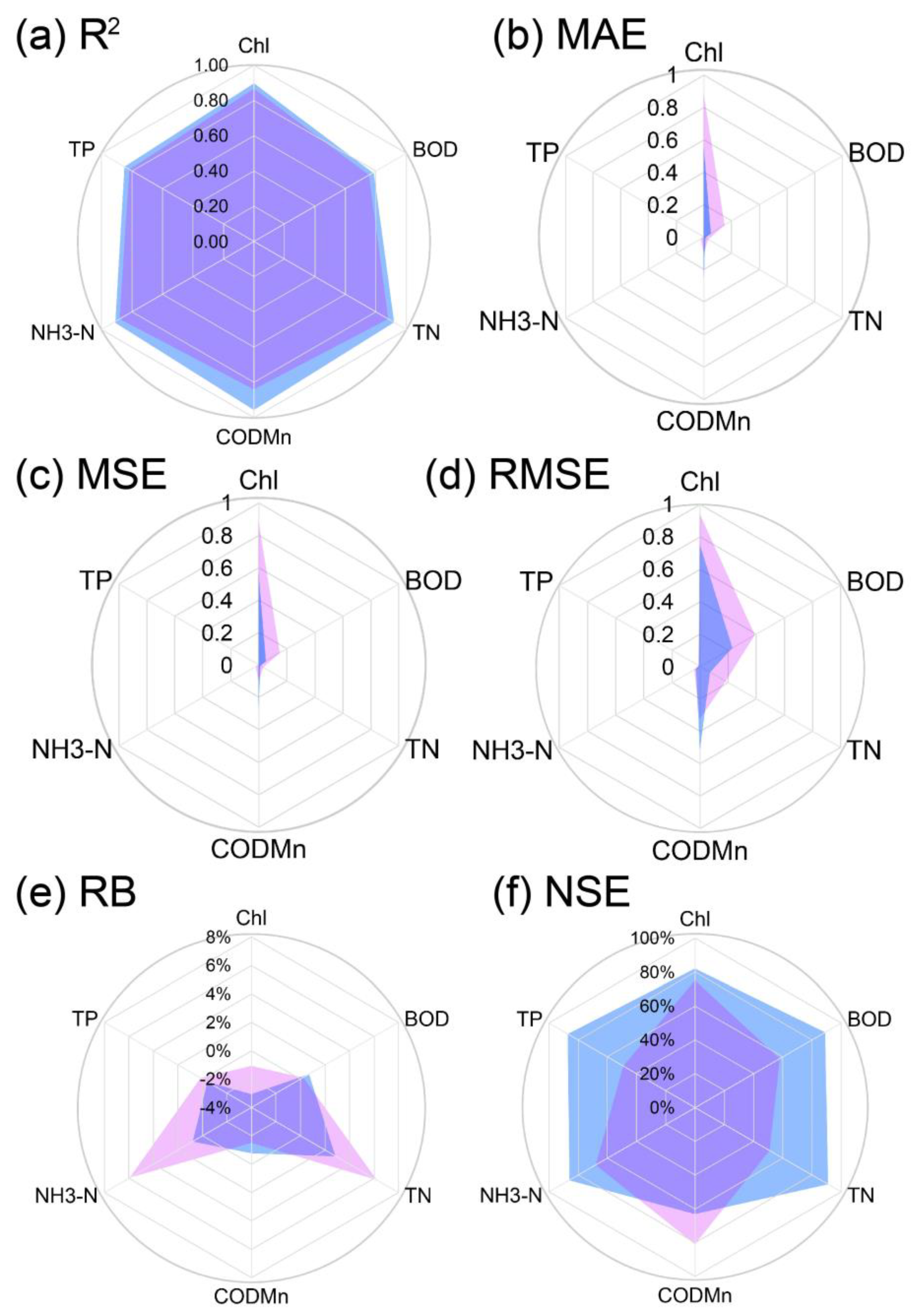
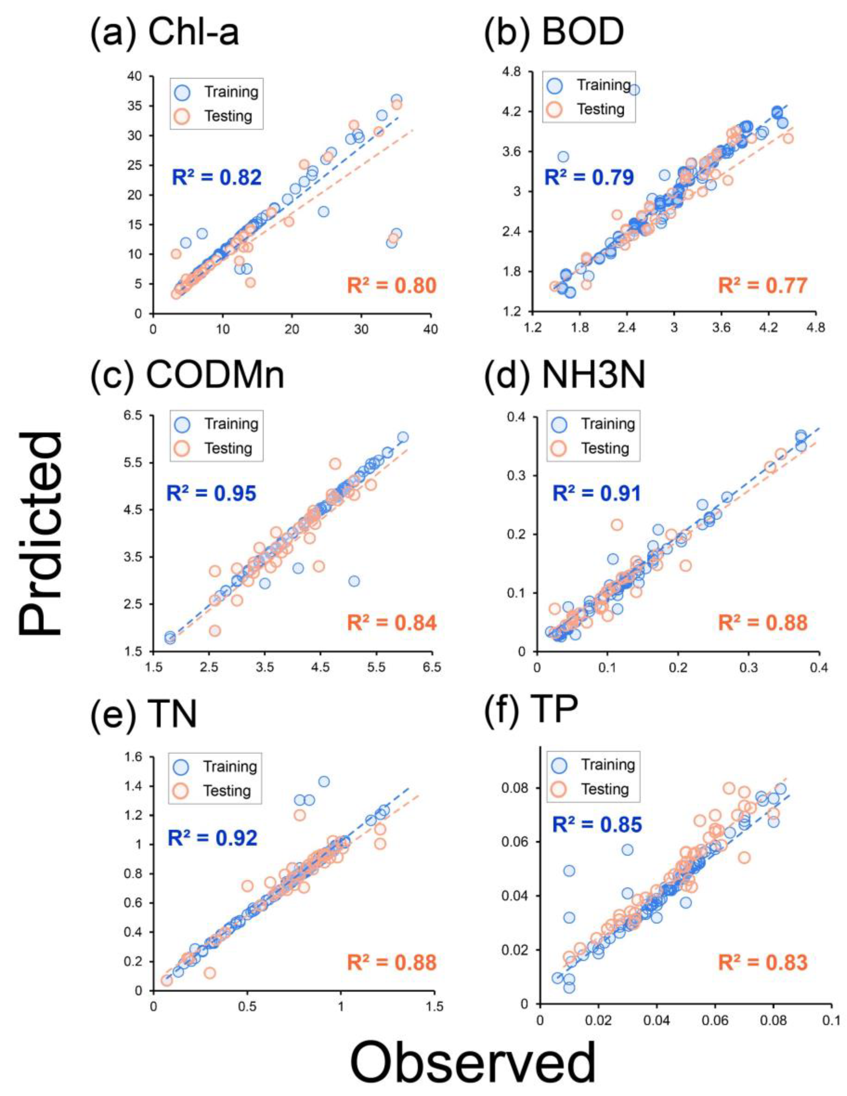
3.1. Evaluation and Regression Results of the ConvLSTM Model

The input dataset applied in the model was made up of 26 variables of spectral data and in situ measurements, combined to produce 138 pairs of satellite observation data. This dataset is partitioned 70% for training (N = 97) and 30% for testing (N = 41). Concentrations of Chl-a, BOD, TN, CODMn, NH3-N, and TP are estimated using the ConvLSTM model, and the regression results for these six parameters are displayed in Figure 3. The modeling technique with ConvLSTM is proven quite accurate, producing R2 values are greater than 0.90 for all the parameters with the training dataset and a mean of 0.80 when applied to the testing dataset. By constituent, the best modeling results are seen when retrieving TN and NH3-N concentrations, followed by CODMn, Chl, TP, and BOD. The model produced mean testing MAE, MSR, and RMSE values of less than 0.20, 0.29, and 0.40 for all water constituents, respectively, and an averaged NSE for testing dataset of more than 0.71. The scattered plots of the observed water quality variables and the data-driven estimations are presented in Figure 4. In addition, the ConvLSTM avoids the overfitting problem to some extent with a relatively small difference in training and testing dataset. The proposed model proposed for BOD generated some errors estimating high values in the testing data. Overall, the model is proven quite powerful in capturing the hidden spectral features, especially for some optically inactive parameters, and successfully estimated a set of parameters, which indicated the utility in solving complex regression problems in water quality.

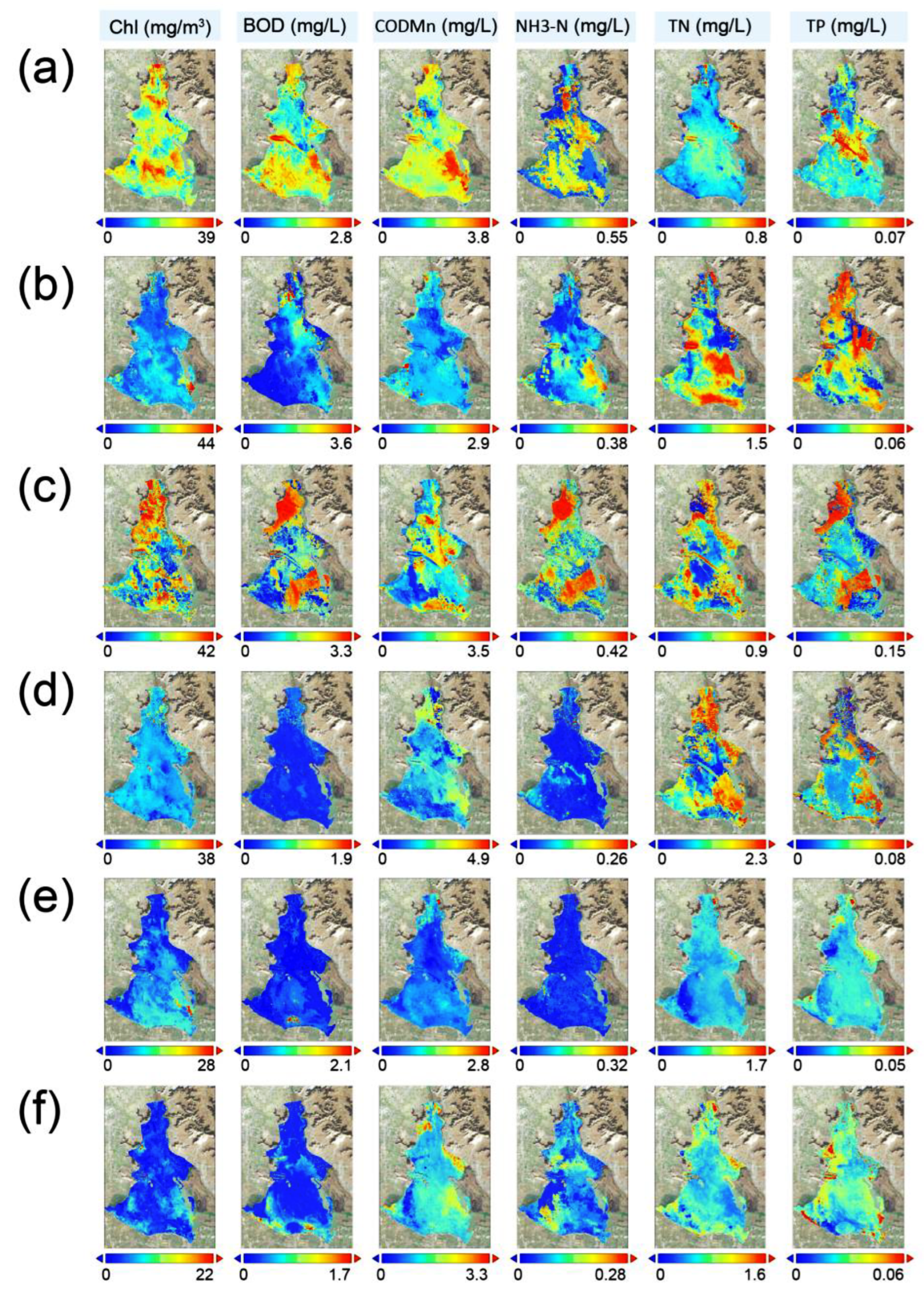
3.2. Water Quality Retrieval for the Landsat 8 OLI Images

The well-trained deep learning model was further applied to generate maps of water quality estimation for all variables derived from the OLI input images. To exhibit the capacity of the proposed model in mapping spatial patterns for water conditions, several scenes of interest for each year from 2013 to 2018 where water quality is inferior to Class III, as specified by the Chinese Environmental Quality Standard for Surface Water (GB3838-2002), were mapped. Figure 5a,b are the estimated water-environment variables on 2013.11.29 and 2014.7.11 where levels of TP and TN, TP, accordingly, are considered to exceed the standard. Scenes on 2015.5.18 with excessive concentration of CODMn (Figure 5c) and on 2016.9.2 for the undesirable level of TP, TN (Figure 5d) were also selected. Excessive concentrations of TP on 2017.11.24 were also identified (Figure 5e), and the last scene on 2018.4.17 was chosen where TN and TP did not meet the Class III standard. With a 30 m resolution of the Landsat 8 OLI images, the distinct spatial variation and pattern can now be clearly identified. There is an obvious difference in nearly all the water constituents between areas around and in the center of the lake such that the concentration around the lake is usually higher than in the middle part, a similar trend found throughout the chosen scenes. In addition, as shown in Figure 5a–c,f, high-value patches tend to cluster in the southeastern and southern parts of the lake. Numerically, three of these scenarios in Figure 5a,c,d have excessive phosphorus concentrations, with mean concentrations of 0.051, 0.094, and 0.054, respectively, the highest exceeding 88% of the phosphorus limit for Class III water (Figure 5c). With the techniques of remote sensing and deep learning, maps of these can better our knowledge of the spatial dynamics and trends in optically active and inactive parameters.

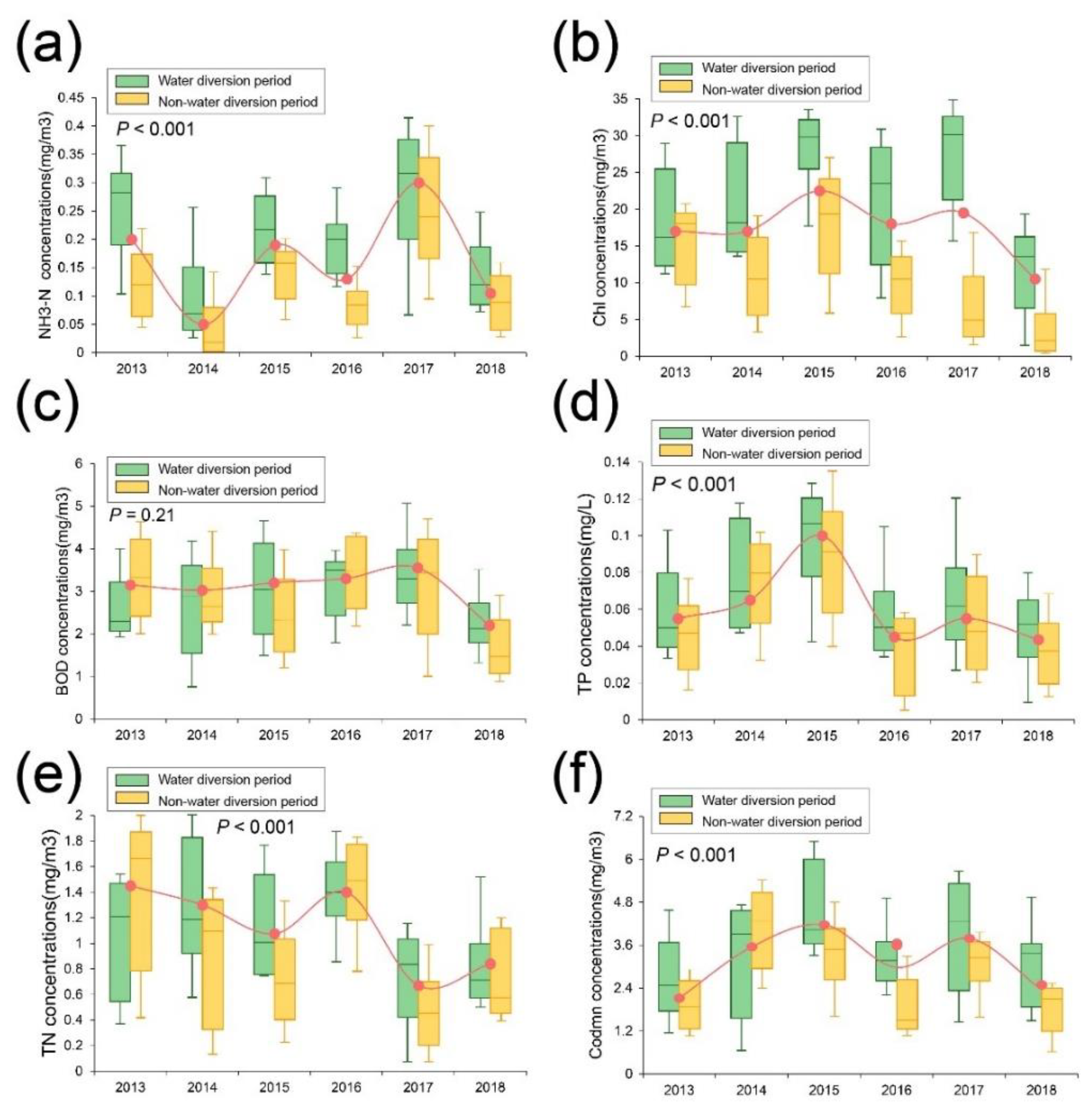
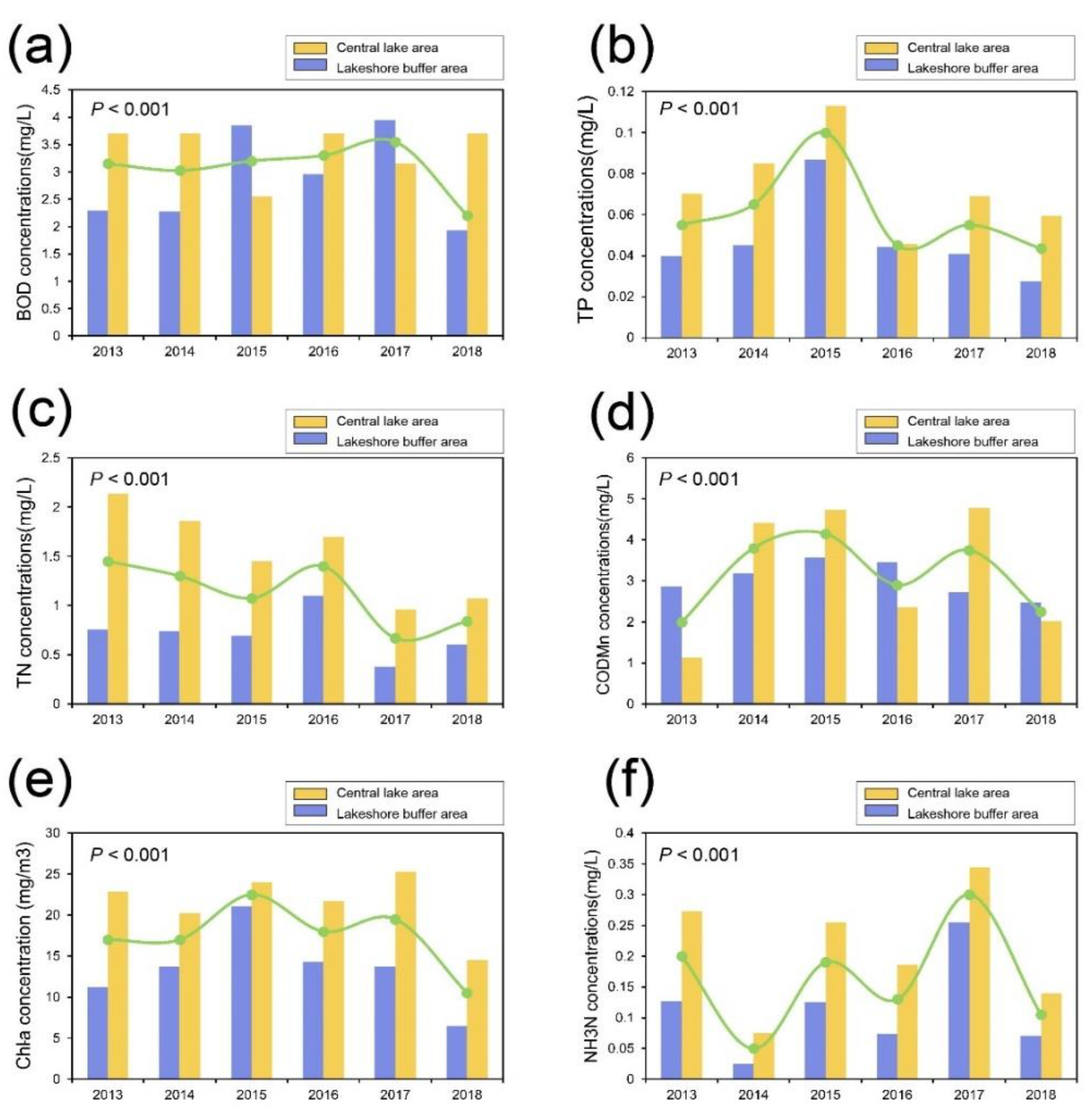
3.3. Spatiotemporal Dynamics of the Model-Retrieved Water Quality Variables

Displayed in the box plots of Figure 6 is the annual average of water quality parameters from 2013 to 2018, applying the ConvLSTM model to the entire OLI dataset. Analysis of the retrieved time series displayed trends in interannual variation and the timing of similar concentration turning points was identified among the variables. Most of the maximum pollution occurred between 2015 and 2016 for TP (0.1 ± 0.02), Chl (22.5 ± 1.42), CODMn (4.15 ± 0.55), TN (1.4 ± 0.23), BOD (3.3 ± 0.35), except a peak concentration for NH3-N (0.3 ± 0.04) in 2017. The results generated an overall decreasing trend for all variables for the studied years. As seen in the results, the temporal dynamics of TP, Chl and CODMn are generally aligned. The xx multiyear average concentration generated for CODMn, BOD and NH3-N in DPL displayed a decrease of 48.47%, 14.5% and 83.75% compared to Class III water limits while an average increase of 21.17% and 12.25% for TP, TN, also regarded as the main pollution factors of DPL, was found. Finally, compared to statistical data on the point scale (i.e., the national monitoring sections), all water constituents estimated on the entire lake area exhibited an increase in concentration, with the highest average increase in chlorophyll concentration 79.09% higher compared to the monitoring data. Finally, the temporal dynamics and trend analysis produced for all parameters on a lake scale might provide new insights into hard-to-observe spatial information, while illustrating the importance of spatial monitoring.
Examination of the one-way ANOVAs detected significant effects of water transfer periods on all water variables except an insignificant water diversion effect on BOD, as seen in Figure 7. Water quality parameters during the water diversion period generally produced higher concentrations in all study years than those in the nondiversion seasons (Figure 7a,b,d–f). The NH3-N and Chl displayed significantly higher values during the water transfer (0.2 ± 0.07 and 25.33 ± 13.58) than the respective lower concentrations of 0.13 ± 0.04 and 9.5 ± 3.67 in seasons without water transfer (p < 0.001). As seen in the results for TP and TN contents (Figure 7d,e), higher levels of pollution are identified in water-transfer seasons ranging from 0.08 ± 0.03 and 1.2 ± 0.62, respectively, compared to those in non-water-transfer seasons (0.05 ± 0.02 and 1.05 ± 0.58). The estimation of CODMn in Figure 7f is also characterized by a significantly higher concentration of 3.8 ± 0.59 during water transfer than that of 2.38 ± 0.520 during other times of the year. In contrast, the results in Figure 7c displayed a higher level of BOD in the non-water-transfer period with a mean concentration of 2.97 ± 1.55 than in the other period (3.5 ± 1.72).
Further exploration of the one-way ANOVAs using two sets of estimations generated for all variables in the central lake area and the lakeshore area (Figure 8) indicated significant spatial effects on water quality (with p values for all parameters less than 0.001). On brief inspection of the spatial statistics, a noticeable difference can be found between the internal and external parts of Dongping Lake based on the location in that the retrieved concentration is identified as a significant decreasing trend from the lake shore to the lake center. For example, the NH3-N content with a mean of 0.21 ± 0.04 mg/L at the lake shore zone is considerably higher than that distributed in the central lake portion with a mean of 0.11 ± 0.03. This is also apparent for TN and TP, the key factors prone to trigger water pollution in Dongping Lake, where the buffer zone around the lake shore show significantly higher concentrations compare to the central area (TN ranging from an averaged of 0.71 ± 0.45 to 1.53 ± 0.79 and TP ranging from an averaged 0.04 ± 0.01 to 0.07 ± 0.03). They displayed strong signals of spatial variations between different portions of the lake, which also align well with water quality maps given in Figure 8. In particular, the retrieved TP for 2015 displays a considerable exceedance (TP with a maximum of 0.05 mg/L for Class III) both in the lakeshore area and the central lake, with 0.063 mg/L and 0.037 mg/L more than the limit value, respectively. Moreover, this is respectively 107% and 169% higher than the average monitoring data for this year. Such spatial dynamics might be connected to the potential pollution sources near the lakeshore and the varying hydrodynamic pattern. In addition, the highly spatially heterogeneous water quality conditions highlight the need for lake-scale monitoring, as field records alone do not appear to be sufficient to detect patterns of pollution that may be at risk of exceedance.

4. Discussion

Utilizing a time series of Landsat 8 OLI dataset, a state-of-the-art deep learning approach was trained and tested for the retrieval of water quality parameters in Dongping Lake from 2013 to 2018 (Figure 1 and Figure 2). Having gained noticeable improvement in recent years, the ConvLSTM method was proven reliable, producing highly accurate predictions for Chl with an R2 of 0.80, BOD of 0.77, TN of 0.88, CODMn of 0.84, NH3-N of 0.88 and TP of 0.83 in this study (Figure 3), which suggest the potential of the technique in addressing water-environment problems. Trends of employing advanced regression methods, such as the SVR, neural networks, and the latest deep learning methodologies, have gained increasing interest among researchers because of their advances in accuracy and reliability, which have seen surging application in different scenarios [16,18,55,60,61,62]. Previous studies on water quality assessment in inland waters have demonstrated the great power of these novel models in capturing the complex nonlinear relationships between water quality variables and ground reflectance and in extracting those spectral features at both low and high levels. The selected optically inactive parameters in this study, such as TN, TP, and NH3-N, were retrieved accurately, among which TN generated even better accuracy than the optically active Chl. Complemented by a series of band arithmetic features by applying expert knowledge [18,63,64,65], as adopted in this study, implementation of the model with a number of spectral features thus enabled the model’s learning of both low-order and high-order interactions through its multilayer architecture for optically active and inactive water variables. This may further validate the hypothesis that the composition of water, in this case, is optically and nonoptically complex. However, the black-box structure of the model might be a potential stumbling block to illustrate the complex interactions in a real environmental system. However, some studies have reported the vanishing gradient problem that might affect modeling capacity, as the magnitude of the gradient decays during backpropagation [66,67]. Therefore, the introduction of a more sophisticated memory mechanism that ensures a stable flow of gradients may further improve the ability and accuracy of spatiotemporal prediction models, as suggested by some recent applications of improved deep learning methods [68,69]. Furthermore, incorporating the laws of pollutant transport, dispersion, and attenuation into the model prediction structure is expected to improve model accuracy and better elucidate the bio-optical properties of specific water bodies.
Previous studies on the trophic state of Dongping Lake have mainly focused on the singular indicator of aquatic health, such as chlorophyll concentration. Some other scholars have successfully applied Landsat series satellites to predict the spatial and temporal evolution of suspended particulate matter (SPM) concentration [7,46,50,70]. These studies have been applied to water quality estimation in specific months or seasons (e.g., the rainy seasons and the dry seasons); however, to the best of our knowledge, a holistic estimation of various water parameters and their temporal–spatial dynamics between the transferred and nontransferred periods of SNWDP-ER in Dongping Lake have rarely been addressed. Applying the trained and tested ConvLSTM model to a range of variables for training and testing datasets, the method shows practically good generalization ability, accurately fitting the high and low values of the in situ measurements (Figure 4). The developed model for BOD, however, underestimates the higher values in the testing data, which might have been linked to the limited monitoring data over the course of several years acquired in this study [14,45,71]. It is therefore beneficial to access and include more water quality observations with longer time series in future research. Another issue of the proposed model is related to adaptation and transferability in other inland waters. With varying hydrological regimes and topographical features, it is possible to produce less accurate water quality estimates than it does in this region. Since the examination of these properties is not the key problem this paper attempts to address, it would be useful to apply the model to additional study areas to provide a larger picture of regional water quality.
The unique hydrological and water-transfer characteristics of the impounded lakes may create different nutrient dynamics from those of general inland lakes. Employing the developed model to the entire DPL generated spatial maps for all variables based on the remotely sensed dataset, which enables further exploration of the temporal–spatial variations of the pollutants from a different perspective. Overall, the model-retrieved time series displayed a general decreasing trend in annual averages from 2013 to 2018 except slight fluctuation of NH3-N (Figure 6), which coincided with previous research on this lake. We further identified the temporal variations in diversion and nondiversion seasons, where all variables display significantly higher values in diversion seasons compared to those in the rest time of the year (p values < 0.001). There is disagreement about the effect of water transfer on water quality, with some researchers suggesting that water quality may be improved by increasing the water inflow thus diluting the originally polluted lake water and improving the eutrophic status of the impounded lakes, and others demonstrating that the resuspension of pollutants such as nitrogen and phosphorus caused by water-transfer practices and the introduction of new polluted water sources may increase the risk of algal outbreaks [2,5,15,72]. It is assumed that the release of nitrogen and phosphorus from the lake sediments due to increased water disturbance has altered the water quality distribution each year. This highlights the need to practice more effective lake management when the water transfer occurs.
The generated maps for water constituents displayed a consistent pattern where the concentration generally decreases from the lake shore to the central lake (Figure 5). This similar pattern is also apparent for most variables throughout the time series, with significantly higher values distributed in the lakeshore area (Figure 8). The dominant cultivated agriculture surrounding the lake and the fish farming within the lake might potentially lead to water degradation and related aquatic issues exacerbated by shallow water environment. Therefore, agricultural management practices and wise aquaculture may be the focus for improving lake water quality [7,15]. The results also identified significant temporal differences in terms of water diversion and nondiversion for the main pollution factors, which showed a clear declining trend from the water transfer period to the nontransfer period (Figure 6 and Figure 7), validated by other findings that the pollution might be more serious when the SWWDP is in operation. The environmental impact of water diversion, which occurs primarily during the dry season, may have outweighed the impact of excess nitrogen and phosphorus compounds in agricultural runoff during the rainy season, with average concentrations of total phosphorus, for example, about 37.5% higher during the transfer period than during the nontransfer period.
Overall, the attempts at developing a water quality estimation model in Dongping Lake are computationally efficient for quantifying the visualizing the temporal dynamic trends for both optically active and inactive variables. The good accuracy produced by this study supports the utility of water quality monitoring based on multispectral data, such as Landsat 8 OLI. The incorporation of spatiotemporal variation detection into the framework may provide a better understanding of the unique dynamics of inland and impounded lakes, thereby facilitating actionable responses to water quality problems.

5. Conclusions

Using the Landsat 8 OLI sensor, remotely sensed datasets on a semimonthly time scale between 2013 and 2018 was produced. Combing the original band spectral information and additional feature extracted from band arithmetic increased the available input data, which is required for the dynamic monitoring system, such as the impounded lakes. In this study, a novel deep learning architecture (ConvLSTM) was developed and tested with multiple metrics, which exhibited good estimation accuracy across optically active and inactive parameters with R2 greater than 0.77 for all water constituents. Applying the proposed ConvLSTM method to all available OLI data for the cross sections used in this study, a time series of retrieved water quality variables were accurately generated. Furthermore, employing the advanced technique to the OLI imagery produced relatively high-resolution spatial maps with ideal spatial coverage across Doping Lake. Spatial distribution maps were found to reflect a similar pattern in all the selected scenarios where concentrations in the center of the lake are usually greater than those in the buffer zone around the lake. In addition, high values tend to cluster in the southeast and south waters. Using the ANOVA and spatial statistics methods variations in temporal and spatial means were identified and analyzed. The results demonstrated distinct differences in water quality between the transfer period and the nontransfer period. Levels of most pollutants are significantly lower during the water diversion months under the operation of the South–North Water Diversion Project (p value < 0.001) except for BOD, and concentrations for all variables are significantly lower in the central portion of the lake (p value < 0.001). These findings highlight the need for actionable measures to address exceedance of priority pollutants (TN and TP) during water transfers. The results also proved the utility of deep learning and remote sensing techniques in water quality monitoring systems. The established workflow may serve as a low-cost but effective method for estimating conventional pollutants in Dongping Lake.

Author Contributions

Conceptualization, H.Z. and B.X.; methodology, H.Z. and B.X.; software, B.X. and G.W.; validation, X.Z.; investigation, X.Z., Q.Z.; resources, B.X. and G.W.; writing—original draft preparation, H.Z.; writing—review and editing, B.X. and G.W.; visualization, X.Z.; supervision, X.Z. and Q.Z.; project administration, G.W. All authors have read and agreed to the published version of the manuscript.

Funding

This study is supported by Major Science and Technology Projects of Inner Mongolia Autono-mous Regions, No.2020ZD0009. And the National Science Fund for Distiguished Young Scholars, No. 52125901.

Data Availability Statement

Landsat 8 images are openly available via www.usgs.gov (accessed on 24 June 2022).

Conflicts of Interest

The authors declare no conflict of interest.

References

  1. Davis, T.W.; Berry, D.L.; Boyer, G.L.; Gobler, C.J. The effects of temperature and nutrients on the growth and dynamics of toxic and non-toxic strains of Microcystis during cyanobacteria blooms. Harmful Algae 2009, 8, 715–725. [Google Scholar] [CrossRef]
  2. Brooks, B.W.; Lazorchak, J.M.; Howard, M.D.; Johnson, M.V.V.; Morton, S.L.; Perkins, D.A.; Reavie, E.D.; Scott, G.I.; Smith, S.A.; Steevens, J.A. Are harmful algal blooms becoming the greatest inland water quality threat to public health and aquatic ecosystems? Environ. Toxicol. Chem. 2016, 35, 6–13. [Google Scholar] [CrossRef]
  3. Boyer; Gregory, L.; Carmichael; Wayne, W. Health impacts from cyanobacteria harmful algae blooms: Implications for the North American Great Lakes. Harmful Algae 2016, 54, 194–212. [Google Scholar]
  4. Walsh, P.; Griffiths, C.; Guignet, D.; Klemick, H. Modeling the property price impact of water quality in 14 Chesapeake Bay counties. Ecol. Econ. 2017, 135, 103–113. [Google Scholar] [CrossRef]
  5. Wang, J.; Fu, Z.; Qiao, H.; Liu, F. Assessment of eutrophication and water quality in the estuarine area of Lake Wuli, Lake Taihu, China. Sci. Total Environ. 2019, 650, 1392–1402. [Google Scholar] [CrossRef]
  6. Gohari, A.; Eslamian, S.; Mirchi, A.; Abedi-Koupaei, J.; Bavani, A.M.; Madani, K. Water transfer as a solution to water shortage: A fix that can backfire. J. Hydrol. 2013, 491, 23–39. [Google Scholar] [CrossRef]
  7. Qu, X.; Chen, Y.; Liu, H.; Xia, W.; Lu, Y.; Gang, D.D.; Lin, L.S. A holistic assessment of water quality condition and spatiotemporal patterns in impounded lakes along the eastern route of China’s South-to-North water diversion project. Water Res. 2020, 185, 116275. [Google Scholar] [CrossRef] [PubMed]
  8. Jiang, J.; Li, S.; Hu, J.; Huang, J. A modeling approach to evaluating the impacts of policy-induced land management practices on non-point source pollution: A case study of the Liuxi River watershed, China. Agric. Water Manag. 2014, 131, 1–16. [Google Scholar] [CrossRef]
  9. Arabi, B.; Salama, M.S.; Pitarch, J.; Verhoef, W. Integration of in-situ and multi-sensor satellite observations for long-term water quality monitoring in coastal areas. Remote Sens. Environ. 2020, 239, 111632. [Google Scholar] [CrossRef]
  10. Wang, S.; Li, J.; Zhang, B.; Lee, Z.; Spyrakos, E.; Feng, L.; Liu, C.; Zhao, H.; Wu, Y.; Zhu, L.; et al. Changes of water clarity in large lakes and reservoirs across China observed from long-term MODIS. Remote Sens. Environ. 2020, 247, 111949. [Google Scholar] [CrossRef]
  11. Liu, G.; Chen, L.; Wang, W.; Sun, C.; Shen, Z. A water quality management methodology for optimizing best management practices considering changes in long-term efficiency. Sci. Total Environ. 2020, 725, 138091. [Google Scholar] [CrossRef] [PubMed]
  12. Sun, H.; Lu, X.; Yu, R.; Yang, J.; Liu, X.; Cao, Z.; Zhang, Z.; Li, M.; Geng, Y. Eutrophication decreased CO2 but increased CH4 emissions from lake: A case study of a shallow Lake Ulansuhai. Water Res. 2021, 201, 117363. [Google Scholar] [CrossRef] [PubMed]
  13. Najah Ahmed, A.; Binti Othman, F.; Abdulmohsin Afan, H.; Khaleel Ibrahim, R.; Ming Fai, C.; Shabbir Hossain, M.; Ehteram, M.; Elshafie, A. Machine learning methods for better water quality prediction. J. Hydrol. 2019, 578, 124084. [Google Scholar] [CrossRef]
  14. Wang, P.; Yao, J.; Wang, G.; Hao, F.; Shrestha, S.; Xue, B.; Xie, G.; Peng, Y. Exploring the application of artificial intelligence technology for identification of water pollution characteristics and tracing the source of water quality pollutants. Sci. Total Environ. 2019, 693, 133440. [Google Scholar] [CrossRef]
  15. Sagan, V.; Peterson, K.T.; Maimaitijiang, M.; Sidike, P.; Sloan, J.; Greeling, B.A.; Maalouf, S.; Adams, C. Monitoring inland water quality using remote sensing: Potential and limitations of spectral indices, bio-optical simulations, machine learning, and cloud computing. Earth-Sci. Rev. 2020, 205, 103187. [Google Scholar] [CrossRef]
  16. Peterson, K.T.; Sagan, V.; Sloan, J.J. Deep learning-based water quality estimation and anomaly detection using Landsat-8/Sentinel-2 virtual constellation and cloud computing. GIScience Remote Sens. 2020, 57, 510–525. [Google Scholar] [CrossRef]
  17. Wang, J.-H.; Li, C.; Xu, Y.-P.; Li, S.-Y.; Du, J.-S.; Han, Y.-P.; Hu, H.-Y. Identifying major contributors to algal blooms in Lake Dianchi by analyzing river-lake water quality correlations in the watershed. J. Clean. Prod. 2021, 315, 128144. [Google Scholar] [CrossRef]
  18. Niu, C.; Tan, K.; Jia, X.; Wang, X. Deep learning based regression for optically inactive inland water quality parameter estimation using airborne hyperspectral imagery. Environ. Pollut. 2021, 286, 117534. [Google Scholar] [CrossRef]
  19. Sun, C.; Chen, L.; Zhu, H.; Xie, H.; Qi, S.; Shen, Z. New framework for natural-artificial transport paths and hydrological connectivity analysis in an agriculture-intensive catchment. Water Res. 2021, 196, 117015. [Google Scholar] [CrossRef]
  20. Sun, X.; Zhang, Y.; Shi, K.; Zhang, Y.; Li, N.; Wang, W.; Huang, X.; Qin, B. Monitoring water quality using proximal remote sensing technology. Sci. Total Environ. 2022, 803, 149805. [Google Scholar] [CrossRef]
  21. Chen, C.; Tang, S.; Pan, Z.; Zhan, H.; Larson, M.; Jönsson, L. Remotely sensed assessment of water quality levels in the Pearl River Estuary, China. Mar. Pollut. Bull. 2007, 54, 1267–1272. [Google Scholar] [CrossRef]
  22. Becker, R.H.; Sultan, M.I.; Boyer, G.L.; Twiss, M.R.; Konopko, E. Mapping cyanobacterial blooms in the Great Lakes using MODIS. J. Great Lakes Res. 2009, 35, 447–453. [Google Scholar] [CrossRef]
  23. Hansen, C.H.; Williams, G.P.; Adjei, Z.; Barlow, A.; Nelson, E.J.; Miller, A.W. Reservoir water quality monitoring using remote sensing with seasonal models: Case study of five central-Utah reservoirs. Lake Reserv. Manag. 2015, 31, 225–240. [Google Scholar] [CrossRef]
  24. Shi, K.; Zhang, Y.; Qin, B.; Zhou, B. Remote sensing of cyanobacterial blooms in inland waters: Present knowledge and future challenges. Sci. Bull. 2019, 64, 1540–1556. [Google Scholar] [CrossRef]
  25. Ho, J.C.; Michalak, A.M.; Pahlevan, N. Widespread global increase in intense lake phytoplankton blooms since the 1980s. Nature 2019, 574, 667–670. [Google Scholar] [CrossRef] [PubMed]
  26. Woolway, R.I.; Kraemer, B.M.; Lenters, J.D.; Merchant, C.J.; O’Reilly, C.M.; Sharma, S. Global lake responses to climate change. Nat. Rev. Earth Environ. 2020, 1, 388–403. [Google Scholar] [CrossRef]
  27. Kloiber, S.M.; Brezonik, P.L.; Olmanson, L.G.; Bauer, M.E. A procedure for regional lake water clarity assessment using Landsat multispectral data. Remote Sens. Environ. 2002, 82, 38–47. [Google Scholar] [CrossRef]
  28. Brezonik, P.; Menken, K.D.; Bauer, M. Landsat-based Remote Sensing of Lake Water Quality Characteristics, Including Chlorophyll and Colored Dissolved Organic Matter (CDOM). Lake Reserv. Manag. 2005, 21, 373–382. [Google Scholar] [CrossRef]
  29. Hadjimitsis, D.G.; Clayton, C. Assessment of temporal variations of water quality in inland water bodies using atmospheric corrected satellite remotely sensed image data. Environ. Monit. Assess. 2008, 159, 281. [Google Scholar] [CrossRef]
  30. Sudheer, K.; Chaubey, I.; Garg, V. Lake water quality assessment from landsat thematic mapper data using neural network: An approach to optimal band combination selection. J. Am. Water Resour. Assoc. 2006, 42, 1683–1695. [Google Scholar] [CrossRef]
  31. McCullough, I.M.; Loftin, C.S.; Sader, S.A. Combining lake and watershed characteristics with Landsat TM data for remote estimation of regional lake clarity. Remote Sens. Environ. 2012, 123, 109–115. [Google Scholar] [CrossRef]
  32. Bonansea, M.; Rodriguez, M.C.; Pinotti, L.; Ferrero, S. Using multi-temporal Landsat imagery and linear mixed models for assessing water quality parameters in Río Tercero reservoir (Argentina). Remote Sens. Environ. 2015, 158, 28–41. [Google Scholar] [CrossRef]
  33. Bonansea, M.; Ledesma, M.; Rodriguez, C.; Pinotti, L. Using new remote sensing satellites for assessing water quality in a reservoir. Hydrol. Sci. J. 2019, 64, 34–44. [Google Scholar] [CrossRef]
  34. Song, K.; Liu, G.; Wang, Q.; Wen, Z.; Lyu, L.; Du, Y.; Sha, L.; Fang, C. Quantification of lake clarity in China using Landsat OLI imagery data. Remote Sens. Environ. 2020, 243, 111800. [Google Scholar] [CrossRef]
  35. Guo, H.; Huang, J.J.; Chen, B.; Guo, X.; Singh, V.P. A machine learning-based strategy for estimating non-optically active water quality parameters using Sentinel-2 imagery. Int. J. Remote Sens. 2021, 42, 1841–1866. [Google Scholar] [CrossRef]
  36. Hao, D.; Asrar, G.R.; Zeng, Y.; Yang, X.; Li, X.; Xiao, J.; Guan, K.; Wen, J.; Xiao, Q.; Berry, J.A. Potential of hotspot solar-induced chlorophyll fluorescence for better tracking terrestrial photosynthesis. Glob. Change Biol. 2021, 27, 2144–2158. [Google Scholar] [CrossRef]
  37. Hao, D.; Asrar, G.R.; Zeng, Y.; Zhu, Q.; Wen, J.; Xiao, Q.; Chen, M. Estimating hourly land surface downward shortwave and photosynthetically active radiation from DSCOVR/EPIC observations. Remote Sens. Environ. 2019, 232, 111320. [Google Scholar] [CrossRef]
  38. Rajaee, T.; Khani, S.; Ravansalar, M. Artificial intelligence-based single and hybrid models for prediction of water quality in rivers: A review. Chemom. Intell. Lab. Syst. 2020, 200, 103978. [Google Scholar] [CrossRef]
  39. Lou, H.; Zhang, Y.; Yang, S.; Wang, X.; Pan, Z.; Luo, Y. A New Method for Long-Term River Discharge Estimation of Small- and Medium-Scale Rivers by Using Multisource Remote Sensing and RSHS: Application and Validation. Remote Sens. 2022, 14, 1798. [Google Scholar] [CrossRef]
  40. Parsaie, A.; Nasrolahi, A.H.; Haghiabi, A.H. Water quality prediction using machine learning methods. Water Qual. Res. J. 2018, 53, 3–13. [Google Scholar] [CrossRef]
  41. Abobakr Yahya, A.S.; Ahmed, A.N.; Binti Othman, F.; Ibrahim, R.K.; Afan, H.A.; El-Shafie, A.; Fai, C.M.; Hossain, M.S.; Ehteram, M.; Elshafie, A. Water Quality Prediction Model Based Support Vector Machine Model for Ungauged River Catchment under Dual Scenarios. Water 2019, 11, 1231. [Google Scholar] [CrossRef] [Green Version]
  42. Gad, M.; Hou, L.; Cao, M.; Adyari, B.; Zhang, L.; Qin, D.; Yu, C.P.; Sun, Q.; Hu, A. Tracking microeukaryotic footprint in a peri-urban watershed, China through machine-learning approaches. Sci. Total Environ. 2022, 806, 150401. [Google Scholar] [CrossRef] [PubMed]
  43. Shi, X.; Chen, Z.; Wang, H.; Yeung, D.-Y.; Wong, W.-K.; Woo, W.-C. Convolutional LSTM network: A machine learning approach for precipitation nowcasting. In Proceedings of the 28th International Conference on Neural Information Processing Systems (NIPS’15), Montreal, QC, Canada, 7–12 December 2015. [Google Scholar]
  44. Claverie, M.; Ju, J.; Masek, J.G.; Dungan, J.L.; Vermote, E.F.; Roger, J.-C.; Skakun, S.V.; Justice, C. The Harmonized Landsat and Sentinel-2 surface reflectance data set. Remote Sens. Environ. 2018, 219, 145–161. [Google Scholar] [CrossRef]
  45. Pu, F.; Ding, C.; Chao, Z.; Yu, Y.; Xu, X. Water-quality classification of inland lakes using Landsat8 images by convolutional neural networks. Remote Sens. 2019, 11, 1674. [Google Scholar] [CrossRef]
  46. Tian, C.; Lu, X.; Pei, H.; Hu, W.; Xie, J. Seasonal dynamics of phytoplankton and its relationship with the environmental factors in Dongping Lake, China. Environ. Monit. Assess. 2013, 185, 2627–2645. [Google Scholar] [CrossRef]
  47. Deng, H.-G.; Zhang, J.; Wu, J.-J.; Yao, X.; Yang, L.-W. Biological denitrification in a macrophytic lake: Implications for macrophytes-dominated lake management in the north of China. Environ. Sci. Pollut. Res. 2020, 27, 42460–42471. [Google Scholar] [CrossRef]
  48. Fang, J.; Yang, R.; Cao, Q.; Dong, J.; Li, C.; Quan, Q.; Huang, M.; Liu, J. Differences of the microbial community structures and predicted metabolic potentials in the lake, river, and wetland sediments in Dongping Lake Basin. Environ. Sci. Pollut. Res. Int. 2020, 27, 19661–19677. [Google Scholar] [CrossRef]
  49. Wu, C.H.; Jiang, C.L. Analysis of evolution mechanism of chloride mass concentration in Dongping Lake and preventive measures. Adv. Sci. Technol. Water Resour. 2021, 41, 15–22. [Google Scholar]
  50. Hu, Z.; Kang, F.; Zou, A.; Yu, L.; Li, Y.; Tian, T.; Kang, G. Evolution trend of the water quality in Dongping Lake after South-North Water Transfer Project in China. J. Groundw. Sci. Eng. 2019, 7, 42–48. [Google Scholar]
  51. Chen, Y.; Chen, S.; Yu, S.; Zhang, Z.; Yang, L.; Yao, M. Distribution and speciation of phosphorus in sediments of Dongping Lake, North China. Environ. Earth Sci. 2014, 72, 3173–3182. [Google Scholar] [CrossRef]
  52. Yao, J.; Wang, G.; Xue, W.; Yao, Z.; Xue, B. Assessing the adaptability of water resources system in Shandong Province, China, using a novel comprehensive co-evolution model. Water Resour. Manag. 2019, 33, 657–675. [Google Scholar] [CrossRef]
  53. Odermatt, D.; Gitelson, A.; Brando, V.E.; Schaepman, M. Review of constituent retrieval in optically deep and complex waters from satellite imagery. Remote Sens. Environ. 2012, 118, 116–126. [Google Scholar] [CrossRef]
  54. Svab, E.; Tyler, A.; Preston, T.; Presing, M.; Balogh, K. Characterizing the spectral reflectance of algae in lake waters with high suspended sediment concentrations. Int. J. Remote Sens. 2005, 26, 919–928. [Google Scholar] [CrossRef]
  55. Hu, Z.; Zhang, Y.; Zhao, Y.; Xie, M.; Zhong, J.; Tu, Z.; Liu, J. A water quality prediction method based on the deep LSTM network considering correlation in smart mariculture. Sensors 2019, 19, 1420. [Google Scholar] [CrossRef]
  56. Sriwongsitanon, N.; Surakit, K.; Thianpopirug, S. Influence of atmospheric correction and number of sampling points on the accuracy of water clarity assessment using remote sensing application. J. Hydrol. 2011, 401, 203–220. [Google Scholar] [CrossRef]
  57. Papoutsa, C.; Retalis, A.; Toulios, L.; Hadjimitsis, D.G. Defining the Landsat TM/ETM+ and CHRIS/PROBA spectral regions in which turbidity can be retrieved in inland waterbodies using field spectroscopy. Int. J. Remote Sens. 2014, 35, 1674–1692. [Google Scholar] [CrossRef]
  58. Zheng, Z.; Ren, J.; Li, Y.; Huang, C.; Liu, G.; Du, C.; Lyu, H. Remote sensing of diffuse attenuation coefficient patterns from Landsat 8 OLI imagery of turbid inland waters: A case study of Dongting Lake. Sci. Total Environ. 2016, 573, 39–54. [Google Scholar] [CrossRef]
  59. Neil, C.; Spyrakos, E.; Hunter, P.D.; Tyler, A.N. A global approach for chlorophyll-a retrieval across optically complex inland waters based on optical water types. Remote Sens. Environ. 2019, 229, 159–178. [Google Scholar] [CrossRef]
  60. Liu, P.; Wang, J.; Sangaiah, A.; Xie, Y.; Yin, X. Analysis and prediction of water quality using LSTM deep neural networks in IoT environment. Sustainability 2019, 11, 2058. [Google Scholar] [CrossRef]
  61. Hafeez, S.; Wong, M.; Ho, H.; Nazeer, M.; Nichol, J.; Abbas, S.; Tang, D.; Lee, K.; Pun, L. Comparison of machine learning algorithms for retrieval of water quality indicators in Case-II waters: A case study of Hong Kong. Remote Sens. 2019, 11, 617. [Google Scholar] [CrossRef]
  62. A, Y.; Wang, G.; Hu, P.; Lai, X.; Xue, B.; Fang, Q. Root-zone soil moisture estimation based on remote sensing data and deep learning. Environ. Res. 2022, 212, 113278. [Google Scholar] [CrossRef] [PubMed]
  63. Guo, Q.; He, Z.; Li, S.; Li, X.; Meng, J.; Hou, Z.; Liu, J.; Chen, Y. Air Pollution Forecasting Using Artificial and Wavelet Neural Networks with Meteorological Conditions. Aerosol Air Qual. Res. 2020, 20, 1429–1439. [Google Scholar] [CrossRef]
  64. Matthews, M.W.; Bernard, S.; Robertson, L. An algorithm for detecting trophic status (chlorophyll-a), cyanobacterial-dominance, surface scums and floating vegetation in inland and coastal waters. Remote Sens. Environ. 2012, 124, 637–652. [Google Scholar] [CrossRef]
  65. Kang, G.; Gao, J.Z.; Xie, G. Data-driven water quality analysis and prediction: A survey. In Proceedings of the 2017 IEEE Third International Conference on Big Data Computing Service and Applications (BigDataService), Redwood City, CA, USA, 6–9 April 2017; pp. 224–232. [Google Scholar] [CrossRef]
  66. Miao, Q.; Pan, B.; Wang, H.; Hsu, K.; Sorooshian, S. Improving monsoon precipitation prediction using combined convolutional and long short term memory neural network. Water 2019, 11, 977. [Google Scholar] [CrossRef]
  67. Tran, H.; Leonarduzzi, E.; De la Fuente, L.; Hull, R.B.; Bansal, V.; Chennault, C.; Gentine, P.; Melchior, P.; Condon, L.E.; Maxwell, R.M. Development of a deep learning emulator for a distributed groundwater–surface water model: ParFlow-ML. Water 2021, 13, 3393. [Google Scholar] [CrossRef]
  68. Wang, Y.; Gao, Z.; Long, M.; Wang, J.; Philip, S.Y. Predrnn++: Towards a resolution of the deep-in-time dilemma in spatiotemporal predictive learning. In Proceedings of the International Conference on Machine Learning, Stockholm, Sweden, 10–15 July 2018; pp. 5123–5132. [Google Scholar]
  69. Wang, Y.; Jiang, L.; Yang, M.-H.; Li, L.-J.; Long, M.; Li, F.-F. Eidetic 3D LSTM: A model for video prediction and beyond. In Proceedings of the International Conference on Learning Representations, New Orleans, LA, USA, 6–9 May 2019. [Google Scholar]
  70. Jiang, T.L.; Zhang, S.Y.; Ding, C.C.; Liu, J.J.; Dai, X.J.; Xu, Y. Analyzing trends of chlorophyll-a concentration in Dongping Lake based on Landsat image from 1985 to 2015. Environ. Monit. China 2018, 2, 137–144. (In Chinese) [Google Scholar]
  71. Sharaf El Din, E. A novel approach for surface water quality modelling based on Landsat-8 tasselled cap transformation. Int. J. Remote Sens. 2020, 41, 7186–7201. [Google Scholar] [CrossRef]
  72. Cui, J.; Zhao, Y.; Sun, W.; Chen, Y.; Wu, B.; Xue, B.; Chen, H.; Li, Z.; Tian, Z. Evaluating the influence of hydrological condition on the phosphorus loads in an agricultural river basin using the SWAT model. Hydrol. Res. 2021, 52, 1143–1158. [Google Scholar] [CrossRef]
Figure 1. A framework for water quality variable retrieval and spatiotemporal analysis based on remote sensing and deep learning techniques.
Remotesensing 14 04505 g001
Figure 2. Geographic locations of the study area in China (a) and in Shandong Province (b), and the spatial distribution of the corresponding national water quality monitoring sections against a Landsat 8 false-color composite image (c).
Remotesensing 14 04505 g002
Figure 3. Results of the regression modeling between OLI-derived spectral properties and the corresponding water quality data from national monitoring sections: (a) R2, (b) MAE, (c) MSE, (d) RMSE, (e) RB and (f) NSE. The blue represents the results from the training period, while the pink represents the results from the testing period.
Remotesensing 14 04505 g003
Figure 4. Plots of the observed versus retrieved water quality concentrations when applying the ConvLSTM methodology to the training and testing datasets: (a) Chl in mg/m3; (b) BOD in mg/L; (c) CODMn in mg/L; (d) NH3-N in mg/L; (e) TN in mg/L and (f) TP in mg/L.
Remotesensing 14 04505 g004
Figure 5. Maps for the estimated water quality variables for Dongping Lake on 2013.11.29 (a), 2014.7.11 (b), 2015.5.18 (c), 2016.9.2 (d), 2017.11.24 (e) and 2018.4.17 (f).
Remotesensing 14 04505 g005
Figure 6. Box plots for averaged water quality parameters estimated by ConvLSTM model for Dongping Lake from 2013 to 2018: (a) BOD in mg/L, (b) TP, (c) TN in mg/L, (d) CODMn in mg/L, (e) Chl in mg/m3 in mg/L and (f) NH3-N in mg/L. The midline of the box indicates the median; bottom and top of the box represent upper and lower quartiles, respectively and the bottom and top whiskers represent 10th and 90th percentiles, respectively.
Remotesensing 14 04505 g006
Figure 7. Temporal variations for Dongping Lake from 2013 to 2018 of (a) NH3-N in mg/L, (b) Chl in mg/m3, (c) BOD in mg/L, (d) TP in mg/L, (e) TN in mg/L and (f) CODMn in mg/L. The green bars represent water quality in the diversion seasons while the yellow ones in nondiversion seasons. The red lines represent the average concentration of water quality components for each year.
Remotesensing 14 04505 g007
Figure 8. Annual average concentrations for the model-retrieved water quality variables for (ae): (a) BOD, (b) TP, (c) TN, (d) CODMn, (e) Chl and (f) NH3-N (the units are consistent with those given earlier). The purple bars represent water quality in the central lake areas, while the yellow ones represent the lakeshore area. The green lines represent the average concentration of water quality components for each year.
Remotesensing 14 04505 g008
Table 1. Water-transfer and non-water-transfer months in Dongping Lake under SNWDP-ER operation.
YearWater-Transfer Period Non-Water-Transfer Period
2013October to DecemberJanuary to September
2014May to JuneJanuary to April,
July to December
2015April to JulyJanuary to March,
August to November
2016January to June, DecemberJuly to November
2017January to May,
October to December
June to November
2018January to May, DecemberJune to November
Table 2. Spectral properties of raw bands and band ratios computed from the Landsat 8 OLI dataset.
Features of Band/Band RatioBand Arithmetic Formula
CoastalOLI Band 1
BlueOLI Band 2
GreenOLI Band 3
RedOLI Band 4
NIROLI Band 5
SWIR 1OLI Band 6
SWIR 2OLI Band 7
CirrusOLI Band 9
Ratio of Green and RedBand 3/Band 4
Ratio of Red and GreenBand 4/Band 3
Ratio of Green and BlueBand 3/Band 2
Ratio of Blue and GreenBand 2/Band 3
Ratio of Red and BlueBand 4/Band 2
Ratio of Blue and RedBand 2/Band 4
Ratio of Red and NIRBand 4/Band 5
Ratio of NIR and RedBand 5/Band 4
Ratio of Green and NIRBand 3/Band 5
Ratio of NIR and GreenBand 5/Band 3
Ratio of Blue and NIRBand 2/Band 5
Ratio of NIR and BlueBand 5/Band 2
Normalized difference Green and Red(Band 3 −Band 4)/(Band 3+Band 4)
Normalized difference NIR and Red(Band 5−Band 4)/(Band 5+Band 4)
Normalized difference NIR and SWIR1(Band 5−Band 6)/(Band 5+Band 6)
Normalized difference Green and NIR(Band 3−Band 5)/(Band 3+Band 5)
Normalized difference SWIR 1 and SWIR2(Band 6−Band 7)/(Band 6+Band 7)
Normalized difference Green and SWIR1(Band 3−Band 6)/(Band 3+Band 6)
Table 3. Statistical and error metrics used for model evaluation.
IndicesAbbreviationFormula
Coefficient of determinationR2 R 2 = 1 i = 1 n y ^ i y i 2 i = 1 n y ¯ i y i 2 (2)
Mean square errorMSE M S E = 1 n i = 1 n y ^ i y i 2 (3)
Root mean square errorRMSE R M S E = 1 n i = 1 n y ^ i y i 2 (4)
Mean absolute errorMAE M A E = 1 n i = 1 n y ^ i y i (5)
Relative errorRE R E = 1 n y ^ i y i y i (6)
Nash–Sutcliffe efficiencyNSE N S E = 1 i = 1 n y ^ i y i 2 i = 1 n y i y i ¯ 2 (7)
Publisher’s Note: MDPI stays neutral with regard to jurisdictional claims in published maps and institutional affiliations.

