Spatiotemporal Variation of Evapotranspiration on Different Land Use/Cover in the Inner Mongolia Reach of the Yellow River Basin

Abstract

The accurate estimation of global evapotranspiration (ET) is essential to understanding the water cycle and land–atmosphere feedbacks in the Earth system. This study focused on the Inner Mongolia Reach of the Yellow River Basin, a typical arid and semi-arid region. Although there are many remote sensing ET datasets, many of the ET algorithms have not considered the impact of soil moisture, especially in water-limited areas. In this paper, the new PT-JPL model, which incorporates soil moisture into ET simulation, is used to improve the accuracy of ET simulation in water-limited areas. The simulation value is evaluated using two Hobq Desert eddy-covariance towers and the Penman–Monteith–Leuning version 2 (PML-V2) dataset. The new PT-JPL model shows the most significant improvements in water-limited regions; the coefficient of determination can reach 0.826, and the RMSE can reduce to 9.645 W/m². Soil evaporation is central to the actual ET increase in the study area. Implementing ecological restoration projects reduced the exposed area of land in the study area and reduced the rate of total ET effectively. Furthermore, the most advanced machine learning local interpretation algorithm—the TreeExplainer-based Shapley additive explanation (SHAP) method—was used to identify the driving factors of ET capacity under different land use types. Temperature, NDVI, and root zone soil moisture were the main environmental factors causing ET changes in different plants. Meanwhile, temperature and root zone soil moisture had a noticeable coupling effect, except for grassland. Furthermore, a threshold effect of temperature to ET was found, and the value is 25, 30, and 30 °C in the forest, grassland, and cropland, respectively. This study provides an essential reference for accurately describing the ET characteristics of arid and semi-arid regions to achieve the efficient management of water resources.

1. Introduction

Evapotranspiration (ET) is an important part of the water cycle, linking energy, water, and circulation [1,2]. ET consumes more than 80% of the precipitation in arid and semi-arid regions and therefore plays a crucial role in the overall hydrological cycle [3,4,5,6,7]. It has been shown that ET is influenced by net radiation [8], wind speed [9], soil moisture stress [10], etc. At the same time, changes in vegetation cover and land use strongly affect hydrothermal balance and have a significant impact on changes in ET. Land use/cover change affects ET by changing vegetation species with different transpiration rates, radiative transfer within the canopy [11,12], topography [13], albedo [14], soil texture [15], apoplastic cover [16], and vegetation cover.

In the 1970s, the large-scale development of intensive agriculture led to severe soil erosion in the upper and middle reaches of the Yellow River Basin, coupled with the conversion of large areas of forest to arable land, low vegetation cover, and fragile ecology [17,18,19]. Since 1999, China has proposed and implemented a series of ecological restoration projects such as the “Grain for Green Project (GfGP)”, and the vegetation cover of the Yellow River basin has increased significantly [20,21], while the large-scale new planting of vegetation has also changed the local water cycle process [22]. Related studies have shown that with the annual increase in vegetation cover, soil erosion in the middle reaches of the Yellow River basin in the Loess Plateau region has significantly decreased [23,24,25,26], but the annual runoff of the Yellow River has dramatically decreased; the ET in the Loess Plateau region has increased substantially, and the regional climate also has become warm drying [27,28]. However, the Inner Mongolian reach of the Yellow River basin shows a decrease in evapotranspiration from year to year, mainly due to the reduction in precipitation and the increase in the degree of drought [5,29]. Therefore, in the Inner Mongolia Reach of the Yellow River Basin, which is strongly influenced by climate type, the study of the intrinsic correlation between ET and vegetation cover/land use is still important and challenging.

Traditional ET monitoring is mainly based on single-point instrument observation, such as the lysimeter method, eddy covariance method, Bowen ratio/energy balance method, eddy-covariance method, etc. [30,31]. Although the above methods can obtain single-point high-precision ET information, they cannot meet the large-scale regional ET research [32]. With the development of remote sensing technology, the surface albedo, vegetation index, and other surface characteristic parameters of large-scale regions can be obtained, and it becomes easier to explore the land surface ET on a large scale [33]. Although hydrological models are available to estimate ET, the complexity and difficulty of obtaining model parameters limit the application of the models. Priestley–Taylor Jet Propulsion Laboratory (PT-JPL) models embedded in remote sensing data can obtain ET at the regional scale with good physical processes that can be distinguished as vegetation transpiration versus soil evaporation [34,35]. In addition, the model does not consider stomatal resistance and wind speed data, and it combines the P–T equation with a new ecophysiological model that converts potential ET into actual ET [35]. Compared with other remotely sensed ET models, the PT-JPL model can be applied on multiple time scales (hourly, daily, monthly, etc.) and spatial scales (point and region) [36,37]. Although the PT-JPL model has been able to meet the needs of different studies, it lacks control of soil moisture [35,38], especially in arid and semi-arid regions where the ET bias simulated by the PT-JPL model is greater [39]. Therefore, combining soil moisture data with the PT-JPL model improves the accuracy of ET simulation in the study area.

In order to examine the influence of climatic factors on regional evapotranspiration and the interaction between different factors, we apply the state-of-the-art continuous learning local interpretation algorithm and the Shapley additive explanation (SHAP) method based on the TreeExplainer [40]. Machine learning algorithms are more suitable for dealing with difficult nonlinear and complex correlation influences than traditional statistical methods [41,42]. Compared with other machine learning methods, the XGBoost model introduces regular terms and column sampling to prevent the occurrence of model overfitting and improve the robustness of the model [43,44]. At the same time, the parallelization strategy is used to increase the computational speed of the model. The XGB–SHAP method based on machine learning algorithms can extract the factors that significantly influence ET from a large amount of data and identify nonlinear interactions.

Long-term, large-scale ET data are vital for studying the water cycle and climate change in arid and semi-arid regions. Therefore, we used the Inner Mongolia Reach of the Yellow River basin as the study area and the PT-JPL model, which incorporates soil water limitations to obtain ET data for a long time series from 1982 to 2015. Additionally, we compared it with the eddy-covariance flux tower measurements data and remote sensing ET products. At the same time, the SHAP method was applied to assess the reasons for the spatial heterogeneity of ET occurring in different sub-bedding surfaces (Figure 1). This study provides an essential reference for accurately describing the ET characteristics of arid and semi-arid regions to achieve the efficient management of water resources.

2. Materials and Methods

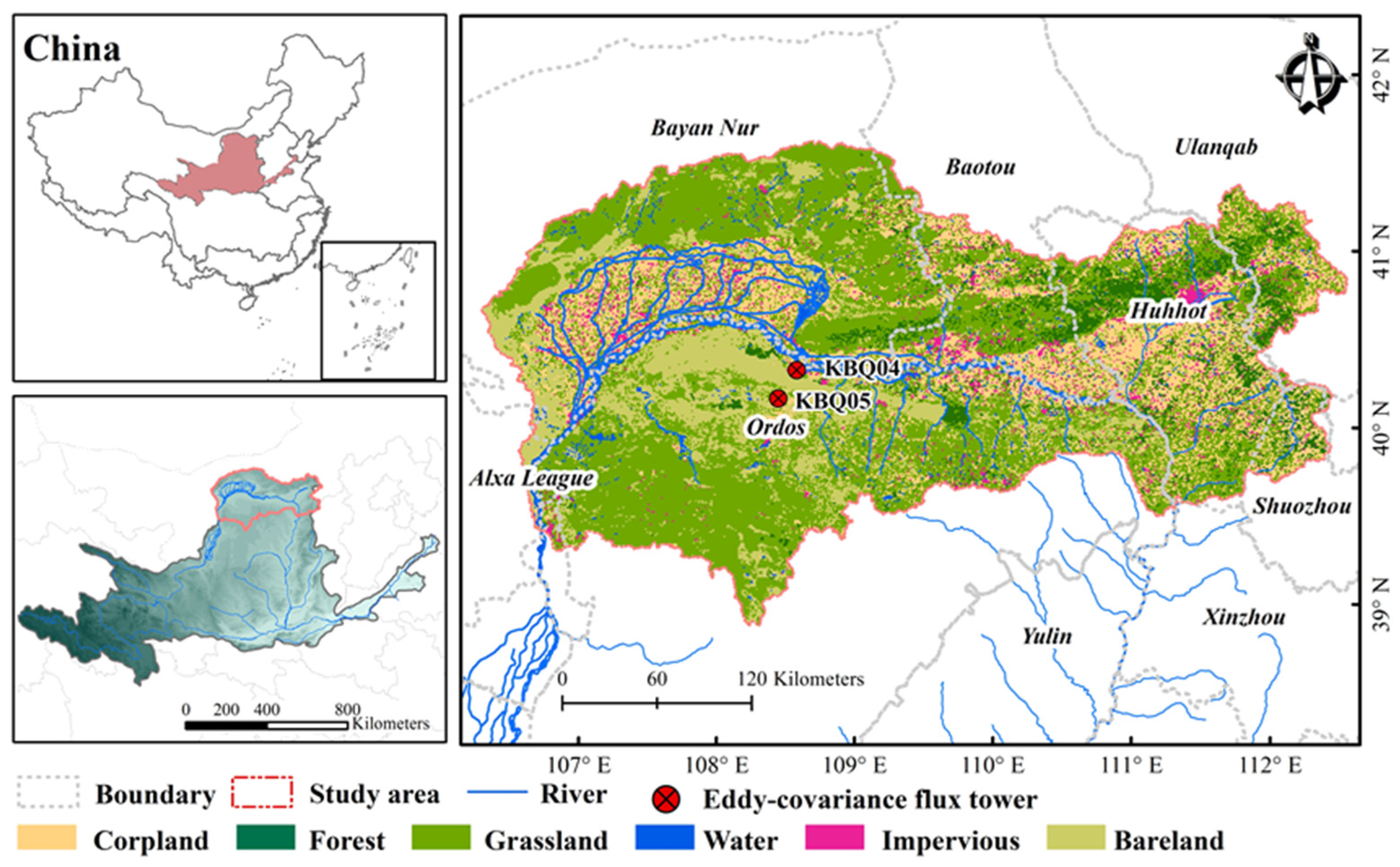
2.1. Study Area

The Inner Mongolia Reach of the Yellow River Basin is located at the northernmost end of the Yellow River Basin (38°~42°N, 106°~112°E); the average altitude is about 1000–1500 m, and the area of drainage is 96,400 km² (Figure 2). In the study area, the major type of vegetation from west to east are grassland and forest. The basin has various geomorphic types, including deserts, plateaus, hills, mountains, and plains. It is located in arid and semi-arid climate areas, with long winters, severe cold, and dry springs. The annual average precipitation is 297.25 mm, the average annual temperature is about 5 °C, and the change in annual evapotranspiration is between 200~300 mm.

2.2. Data Preparation

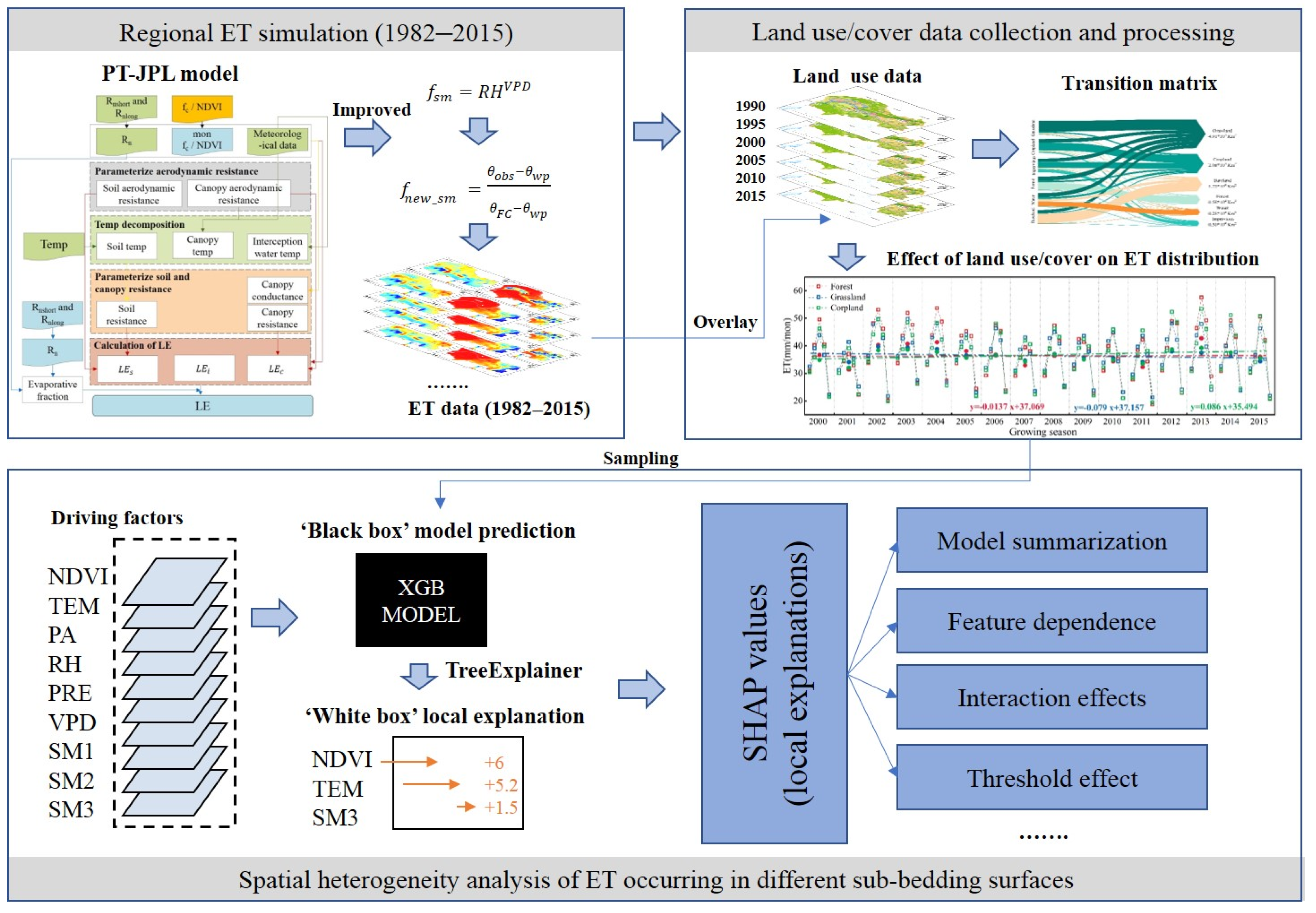
In this study, we obtained land use data for 1990, 1995, 2000, 2005, 2010, and 2015 with a resolution of 1 km from the Institute of Geographic Sciences and Natural Resources Research, China (http://www.resdc.cn/, accessed on 30 December 2021). The land use/land cover (LULC) data used in this paper were produced by Jiyuan Liu’s team at the Institute of Geographical Sciences and Natural Resources Research, the Chinese Academy of Sciences. The dataset is based on Landsat 8, GF-2, and other remote sensing data. The land use data from 1990 to 2015 were obtained by constructing a high-resolution remote sensing–UAV–ground survey and observation technology system, combined with a human–machine interactive interpretation method. This dataset is unified and integrated, quality checked, and finally evaluated by a confusion matrix for classification accuracy and total accuracy. Among them, the comprehensive evaluation accuracy of the primary type reaches more than 93%, and the secondary classification can reach more than 90% [45,46,47,48]. It was divided into six main categories: cropland, forest, grassland, water bodies, impervious, and bare land.

The data driving the PT-JPL model comprise the following: Meteorological data (precipitation, temperature, air pressure, wind speed) for the period from 1979 to 2015, which were obtained from the China Meteorological Forcing Dataset (CMFD) (http://data.tpdc.ac.cn/, accessed on 30 December 2021). The data range covers the whole Chinese mainland with a spatial resolution of 0.1° × 0.1°; the time resolution is one month. Radiation data (net longwave radiation and net shortwave radiation) was obtained from the fifth-generation European Centre for Medium-Range Weather Forecasts (ECMWF) atmospheric reanalysis (ERA5) (https://cds.climate.copernicus.eu/, accessed on 30 December 2021). The data range covers worldwide with a spatial resolution of 0.25° × 0.25°; the time resolution is one month. At the exact times, we also obtained the long-time series vegetation data, including the normalized difference vegetation index (NDVI) data from global inventory modeling and mapping studies (GIMMS) (https://glam1.gsfc.nasa.gov, accessed on 30 December 2021). The data have a spatial resolution of 0.083° × 0.083°; the time resolution is 15 days. The maximum value composite method was used to synthesize monthly data from 15 days of NDVI data.

To evaluate the performance of the PT-JPLnew model, we used data from two flux tower sites in the Hobq Desert (KBQ04 and KBQ05) (Figure 2). The flux station data are half-hourly instantaneous data from 2006 to 2009, which are averaged to obtain daily average data. Then, all daily data in that month are averaged to obtain monthly latent heat flux data. The data set Penman–Monteith–Leuning version 2 (PML-V2) [49], which includes vegetation transpiration (E_c), soil evaporation (E_s), vaporization of intercepted precipitation (E_i), and water body and snow evaporation (ET_water), was used to validate the accuracy of the evapotranspiration component simulation by the new PT-JPL model. The PML-V2 datasets have 16 years (2002 to 2017) of global ET data sets, spatial resolution of 500 m, and time resolution of 8 days (

Table 1. PT-JPL model-driven and validation data.

Variable	Product Name	Time Range	Time Resolution	Spatial Resolution
meteorological data	CMFD	1982–2015	Monthly	0.1° × 0.1°
Net radiation	ERA5	1982–2015	Monthly	0.25° × 0.25°
Relative humidity	ERA5	1982–2015	Monthly	0.25° × 0.25°
NDVI	GIMMS	1982–2015	15 d	0.083° × 0.083°
Soil moisture	GLDAS	1982–2015	Monthly	0.25° × 0.25°
ET	PML-V2	2002–2017	8 d	500 m × 500 m

.). All data for one month are averaged and then multiplied by the number of days in the month to obtain the monthly ET data. All of the remotely sensed data were resampled to 0.083° resolution to match the spatial resolution of NDVI data to better reflect the effect of vegetation change on local ET.

2.3. Method

2.3.1. PT-JPL ET Algorithm

The PT-JPL ET algorithm applies ecophysiological constraints to model reductions of ET from the atmospheric potential ET due to sub-optimal environmental conditions [35]. The model effectively solves the difficulty of obtaining ground impedance data in ET simulations. Additionally, the model contains a lot of plant physiological parameters, which can effectively reflect the changes of ET or latent energy (LE) caused by vegetation changes in the study area. ET and latent heat (LE) are the links between the water cycle and energy cycle, so there is ET λ = $LE$. The PT-JPL model can divide the ET into three parts: vegetation canopy transpiration ($L{E}_c$), soil evaporation ($L{E}_s$), and vegetation canopy interception evaporation ($L{E}_i$). The algorithm can be describe as:

$$LE=L{E}_s+L{E}_c+L{E}_i$$

(1)

$$L{E}_s=\left[f_{wet}+f_{sm}\times \left(1-f_{wet}\right)\right]\times \frac{\Delta }{\Delta +\gamma }\times \alpha \times \left(R_{ns}-G\right)$$

(2)

$$L{E}_c=\left(1-f_{wet}\right)\times f_g\times f_T\times f_M\times \alpha \frac{\Delta }{\Delta +\gamma }{R}_{nc}$$

(3)

$$L{E}_i=f_{wet}\times \alpha \times \frac{\Delta }{\Delta +\gamma }{R}_{nc}$$

(4)

where $f_{wet}$ is relative surface humidity (dimensionless) and $f_{wet}=R{H}^4$; RH is the relative humidity of air (%); $f_{sm}$ is soil moisture constraint (dimensionless); $f_g$ is green canopy fraction (dimensionless); $f_T$ is planted temperature constraint (dimensionless), and $f_M$ is plant moisture constraint (dimensionless); $\alpha$ is the Priestley–Taylor coefficient that is set as 1.26; Δ is the slope of the saturated vapor–pressure relationship (kPa/°C); γ is the psychrometric constant (kPa/°C); G is the ground heat flux (W/m²); λ is the latent heat of vaporization (MJ/kg); $R_n$ is the net radiation (W/m²), ($R_n=R_{nshort}+R_{nlong}$), $R_{nshort}$ is net shortwave radiation (W/m²), and $R_{nlong}$ is net longwave radiation (W/m²); $R_{ns}$ is the net radiation reaching the soil surface (W/m²), $R_{ns}=R_n\exp \left(-k_{R_n}LAI\right)$, $k_{R_n}$ the extinction coefficient, taken as 0.6; and $R_{nc}$ is the net radiation intercepted in the canopy (W/m²), $R_{nc}=R_n-R_{ns}$ [39,50]. For further detailed reference, see Fisher et al., 2008.

In this model,

$$f_g=\frac{f_{APAR}}{f_{IPAR}}$$

(5)

$$f_m=\frac{f_{APAR}}{f_{APA{R}_{max}}}$$

(6)

$$f_t=\exp \left[-{\left(\frac{T_a-T_{opt}}{T_{opt}}\right)}^2\right]$$

(7)

where $f_{APAR}$ is the fraction of absorbed photosynthetically active radiation, $f_{IPAR}$ is the fraction of intercepted PAR, $T_a$ is the maximum daily air temperature, and $T_{opt}$ is the optimum temperature [39].

$$f_{sm}=R{H}^{VPD}$$

(8)

where soil water control on evaporation is implicitly represented through the upper formula. However, in some arid and semi-arid areas, soil moisture is the main limiting factor of ET compared with vapor pressure deficit (VPD) [32]. Therefore, we used the soil moisture to modify model parameters $f_{sm}$ [39]:

$$f_{new\_sm}=\frac{{\theta }_{obs}-{\theta }_{wp}}{{\theta }_{FC}-{\theta }_{wp}}$$

(9)

where ${\theta }_{obs}$ is the soil moisture observation, ${\theta }_{wp}$ is the soil–plant wilting point, and ${\theta }_{FC}$ is the soil field capacity. Due to the lack of long-term measured soil water data, the Global Land Data Assimilation System (GLDAS) soil moisture dataset is used to replace ${\theta }_{obs}$ [51]. Soil properties extracted from the Harmonized World Soil Database version 1.2.1 (HWSD 1.21) include the porosity and the wilting point. This paper combined the new PT-JPL model with remote sensing data to obtain the ET from the regional scale. We use this method to find out the main factors affecting the change in ET in the Inner Mongolia Reach of the Yellow River Basin. The spatial resolution of all data is unified, as the NDVI data’s spatial resolution is 0.083° × 0.083°, and the time resolution is one month.

2.3.2. Extreme Gradient Boosting Method (XGB)

Chen and Guestrin [52] first proposed the Tree-based machine learning model XGB method; it is one of the integrated learning methods that combine multiple learning models, so that the XGB method can obtain better prediction results. Compared with deep learning models, the tree-based model’s performance is better on tabular datasets [40]. The algorithm utilizes CART as the base classifier and is jointly decided by multiple related decision trees. It can solve most regressions and classifications; one of the critical applications is data feature mining and analysis. This method can perform multithreaded calculations and scale the newly added weight at each pressurization step using shrinkage technology to avoid overfitting [40].

Therefore, the nonlinear XGB algorithm is to simulate monthly ET from different drivers, including temperature (TEM, °C), precipitation (PRE, mm), vapor pressure deficit (VPD, hPa), air pressure (PA, Pa), relative humidity (RH, %), NDVI, surface soil moisture (SM1, m³/m³), soil moisture at 10–40 cm (SM2, m³/m³), and soil moisture at 40–100 cm (SM3, m³/m³). There were 90,675 samples of monthly combinations of the iterative decision tree model, with a sample number of 6516 forests, a sample number of 60,316 grasslands, and a sample number of 23,843 farmlands. We need to input a sample size as large as possible to obtain reliable results.

2.3.3. Explainable Predictions: Shapley Additive Explanations

With the development of machine learning algorithms in feature extraction and prediction, the prediction process has been regarded as the ‘black box’, and the lack of enough interpretability has led to doubt [53,54]. We applied the state-of-the-art TreeExplainer-based SHAP framework, presented by Lundberg et al., to analyze the primary factors and threshold of the ET in different land use covers [55]. The XGB–SHAP framework has successfully been applied to the local explanations of human disease and socioeconomic sciences [56,57]. Based on the classical game-theoretic Shapley values inthe previous model-agnostic work, the TreeExplainer realized optimal local interpretation, enabling us to better understand the impact of individual features on model losses. The Shapley additive explanation (SHAP) interaction values use the ‘Shapley interaction index’ to capture local interaction effects. By calculating the average marginal impact of many possible factors on the predicted value, SHAP assigns the expected significant value to each feature to provide a theoretical basis for the subsequent interaction effect calculation. Through the SHAP method, the factor effect, main effect, and coupling effect between different factors influencing the land use mechanism on ET can be interpreted easily.

3. Results

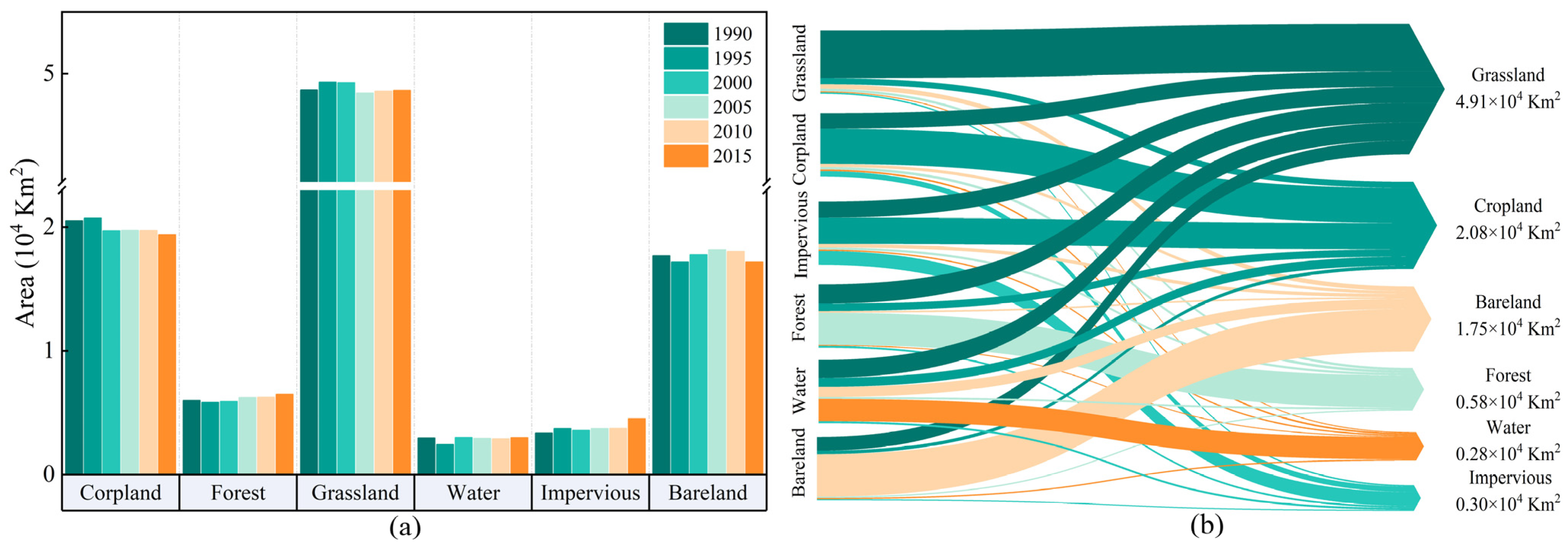
3.1. The Area Variations and Transfer Direction of the Land Use in the Inner Mongolia Reach of the Yellow River Basin

The extent of the different land types in the Inner Mongolia Reach of the Yellow River Basin between 1990 and 2015 are shown in Figure 3. Over the past 30 years, the area of the other land types has barely been unchanged. Grassland, cropland, and bare land are the main types of land use, but the impervious area shows a rising trend year by year. Although the Chinese government has implemented several ecological restoration measures since 1999, the total area of forest and grassland is almost unchanged. Therefore, combining the land use transfer matrix is necessary to analyze the effect of GfGP comprehensively. As shown in Figure 3b, the impervious area and forest showed the most change over the study period, with up to 41.2% of the impervious area converted to cropland and 30.6% of the forest area converted to grassland. Although the forest area has risen, the increase is slight. However, the water area showed a decreasing trend year after year. Additionally, the proportion of different land use types converted to water area is small. Therefore, it is necessary to study the ET laws under different land use types in this water deficiency region.

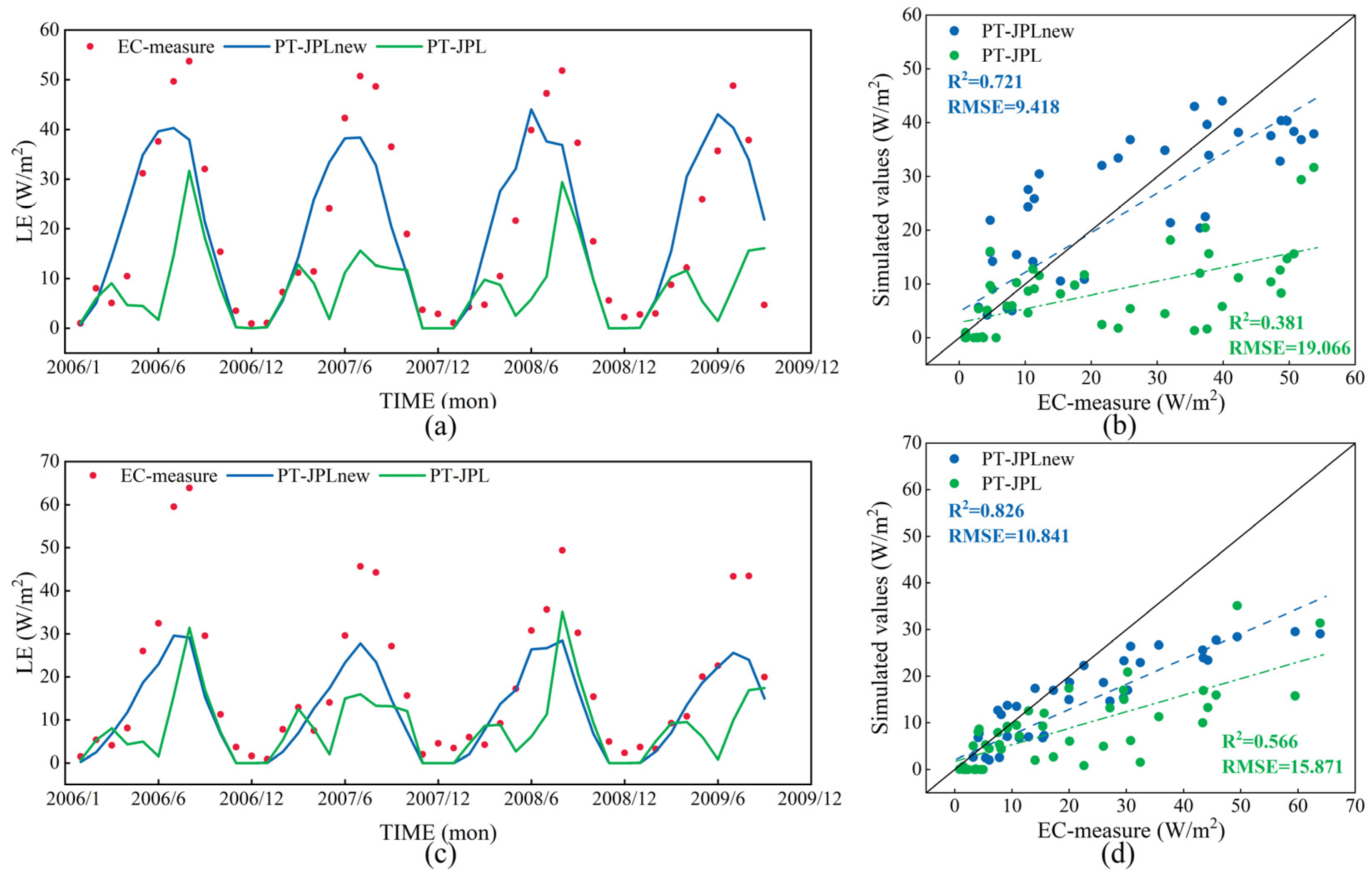
3.2. Model Validation

Figure 4 compares the latent heat flux measured at the flux station (KBQ04 and KBQ05) with PT-JPL and the new PT-JPL. Figure 4a,c shows the time-series process, and Figure 4b,d shows the comparison diagram of simulated value and measured value before and after model improvement. The blue dot represents the simulation value of the new PT-JPL model, and the green dot represents the simulation value of the PT-JPL model. The diagonal is the line y = x; the closer to this line, the closer the simulation effect is to the measured value and the better the simulation effect is. The results show that, compared with the original model, the improved model could well reflect the change process of latent heat flux in time; the original model underestimated the growing season [58,59]. According to the value of coefficients of determination (R²) and root mean square error (RMSE), the new PT-JPL model improves the accuracy of the model to a certain extent, and the simulated LE is closer to the actual value. For example, at site KBQ04, the R² has almost doubled from 0.381 to 0.721, and the RMSE has fallen from 19.066 W/m² to 9.418 W/m². However, the simulated ET value is always underestimated during peak growing season (i.e., June–August). This is because our study area is an arid and semi-arid region with perennial water scarcity, and precipitation is the only water source in the region. Once ET exceeds precipitation, it will result in less available water in the soil, reducing runoff and ultimately negatively affecting groundwater storage. Meanwhile, despite the introduction of soil moisture data in the new PT-JPL model, there is a certain underestimation of remotely sensed soil water data products compared with the actual measured soil water data.

A further validation of the PT-JPLnew model’s accuracy on a different component with the data of PML-V2 LE in the same period was taken (Figure 5). To the vegetation canopy transpiration $E_c$, the correlation coefficient in most regions is higher than 0.8. In about 45% of areas, the correlation of soil evaporation $E_s$ exceeded 0.5. The correlation is higher in the northwest and lowers in the southeast. According to Figure 2, negative values mainly appear in the cropland area. Due to the forest being distributed primarily on the southeastern margin of the study area, the simulation $E_i$ is mostly in these places. Although the region is small, the scope of the correlation exceeded 0.4, about 50%. Although we considered the influence of soil moisture on the model, we did not consider the influence of farmland irrigation on ET simulation. However, the PML-V2 model considers the effects of stomatal conductance and atmospheric CO₂ concentration on vegetation carbon and water processes. The PML-V2 model has a spatial resolution of 500 m, which is more accurate, but the PT-JPL model results correlate well. In general, the new PT-JPL model shows good performance on time and space scales, and the simulation results in this paper are reliable.

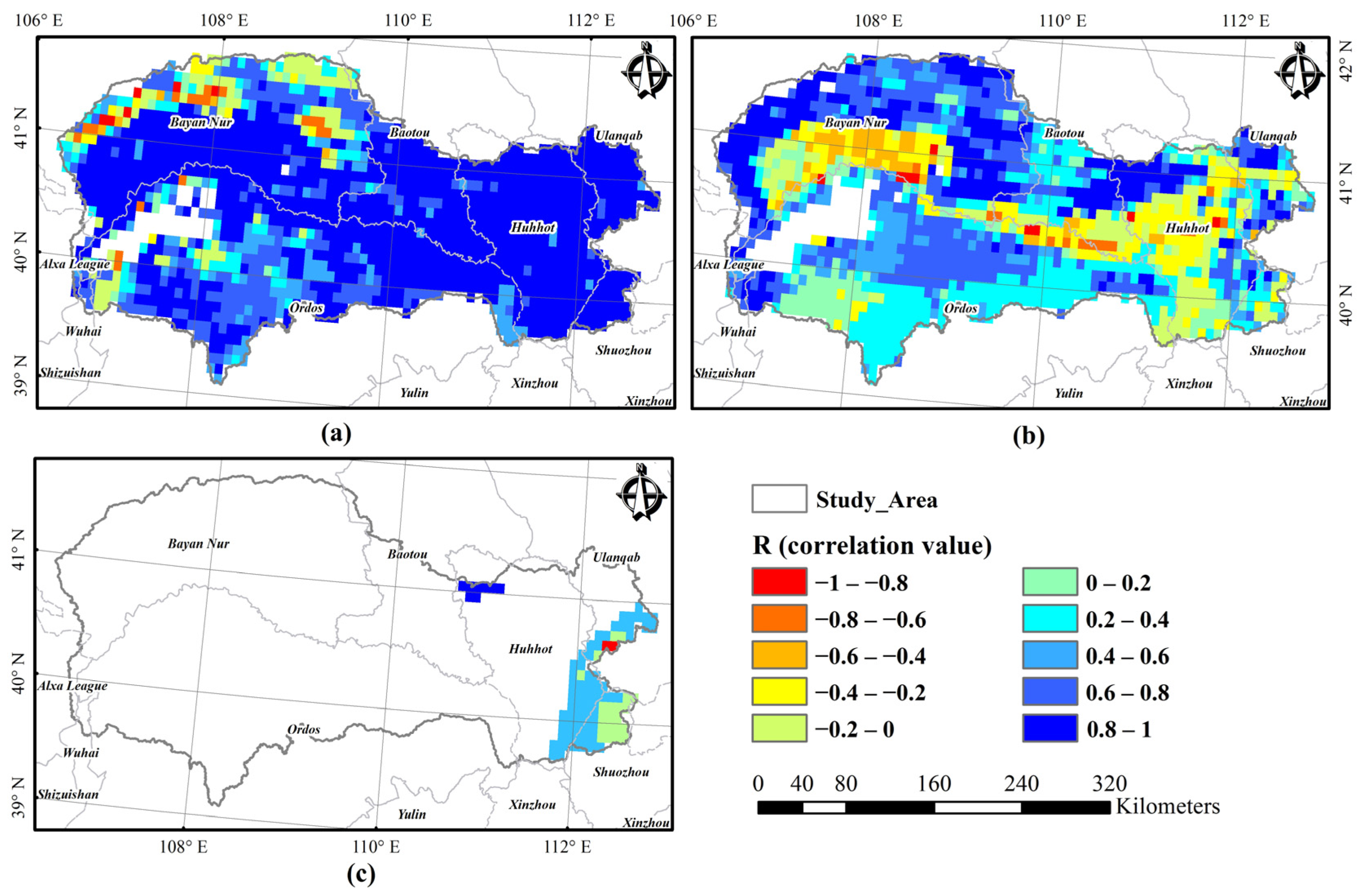
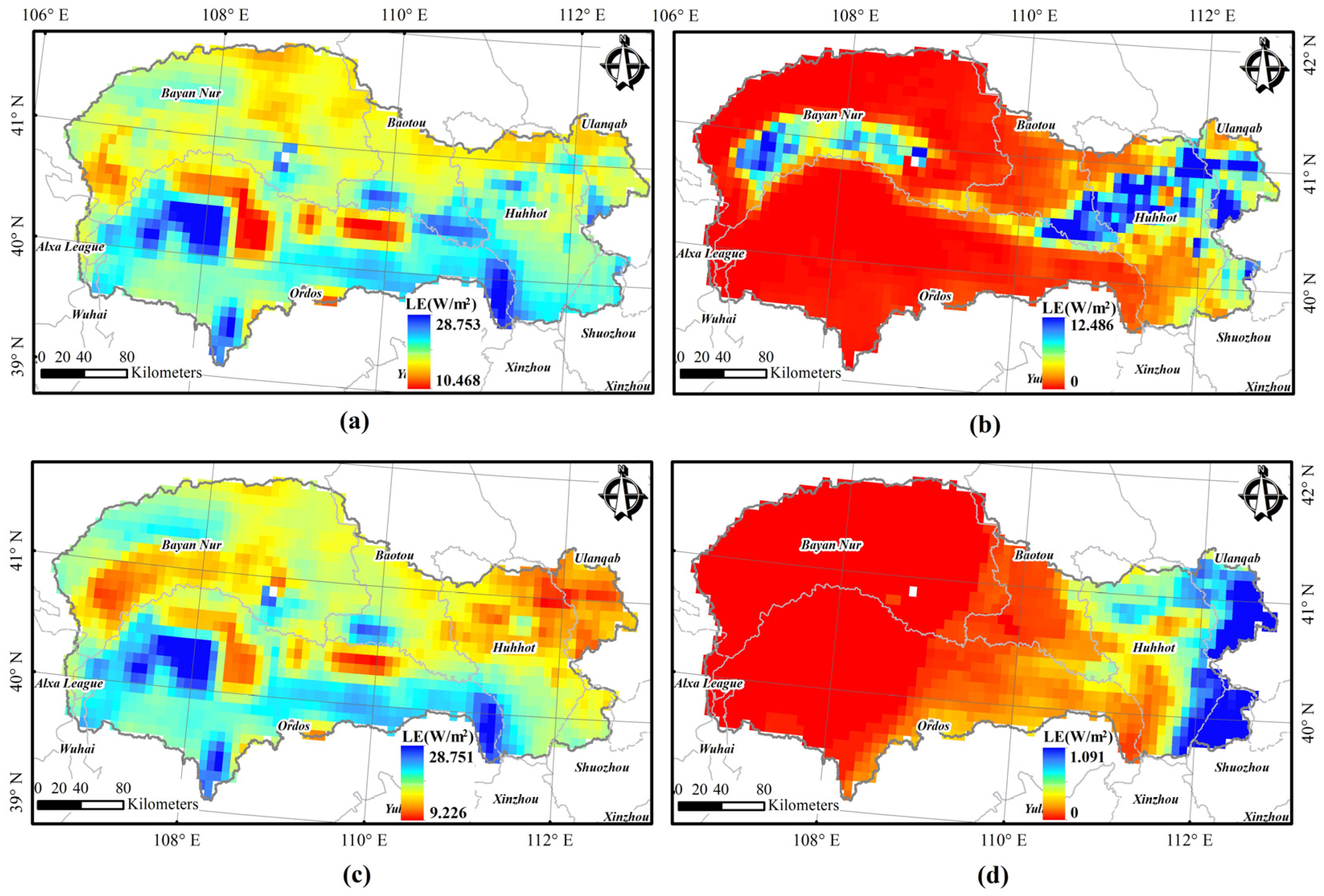
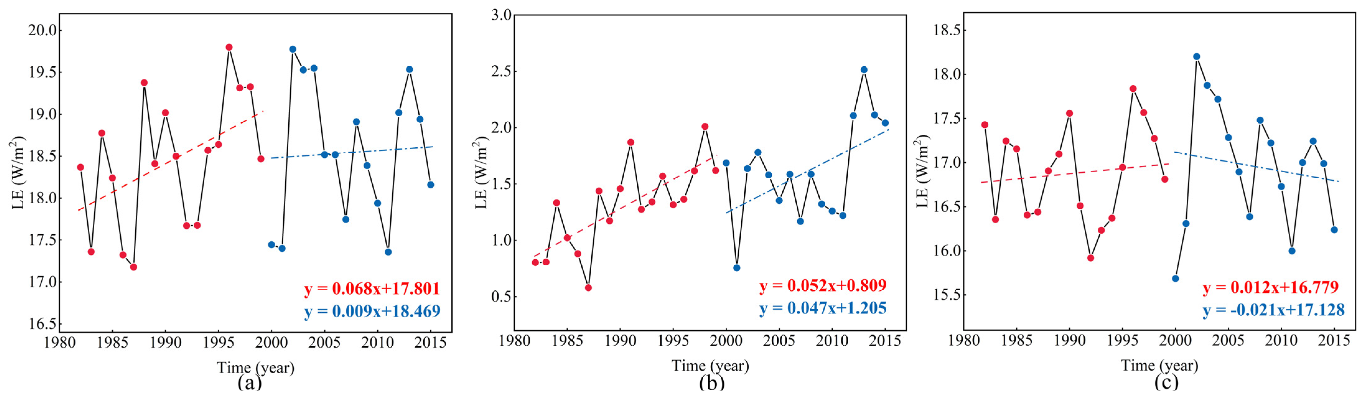
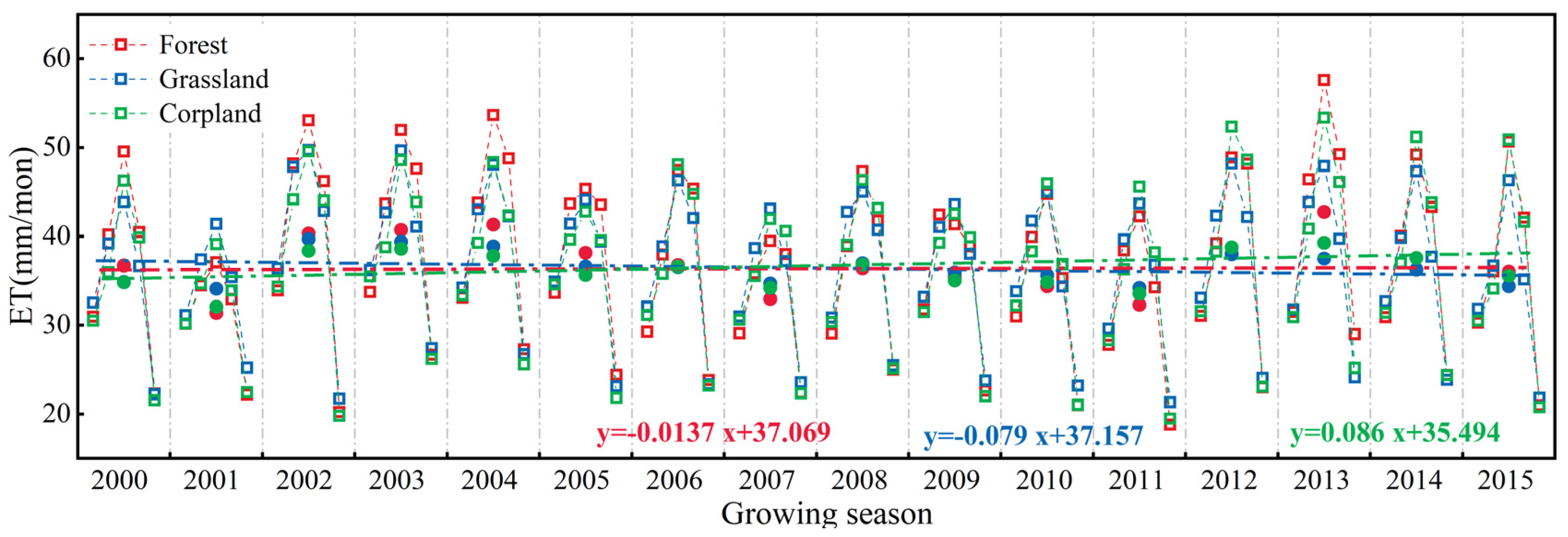
3.3. Spatiotemporal Variations in Regional ET

Figure 6a shows the spatial distribution of multiyear-averaged ET under different land use/cover. The total actual ET is high in the south and low in the north; the lowest value occurs in bare land areas with low vegetation coverage (Figure 2). Vegetation transpiration ($L{E}_c$) is also an essential part of regional water consumption, but the vegetation types in this area are mainly grassland and cropland. Therefore, the high $L{E}_c$ value area primarily occurs in the Hetao Irrigation Area, cropland and forest east of the study area (Figure 2). The forest is mainly distributed east of the study area, so the vegetation canopy interception evaporation ($L{E}_i$) is mainly concentrated here. Still, the LE_i value of the multiyear average is very low—perhaps 1 W/m² (only 12 mm/year). Another critical component of ET is soil evaporation; from the spatial distribution of Figure 6c, soil evaporation ($L{E}_s$) is low in cropland and forest-covered areas. The vegetation coverage here is extensive. The western region of the study area is mainly grassland because the vegetation is sparse in this area; the larger the soil area exposed, the greater the solar radiation reaching the ground, so the more significant the soil evaporation.

As stated above, we can obtain the spatial distribution of the total actual ET and different ET components. However, it cannot reflect the change across the entire temporal variety of ET in the study area. Therefore, based on the spatial analysis, we calculated the statistics of the time series of multiyear latent heat values during the 1982–2015 period to comprehensively analyze the effect of GfGP. Meanwhile, the $L{E}_c$ and $L{E}_s$ are the main components of the total LE in this study, so the time variation of these three parts was mainly analyzed (Figure 7).

Taking 1999 as the boundary, we compared the temporal changes of actual evapotranspiration ($LE$), vegetation transpiration ($L{E}_c$), and soil evaporation ($L{E}_s$) between 1982–1999 and 2000–2015. During the study period, the total actual ET, vegetation transpiration, and soil evaporation of the study area almost continuously increased from 1982 to 2015. After 1999, the increase rate of LE reduced from 0.068 W/m² to 0.009 W/m², and the increase rate of $L{E}_c$ reduced from 0.052 W/m² to 0.047 W/m². Surprisingly, the increase rate of $L{E}_s$ reduced from 0.012 W/m² to −0.021 W/m². It shows that the ecological restoration measures effectively reduced the exposed area of land in the study area and reduced the rate of total LE. In general, soil evaporation ($L{E}_s$) is central to the actual ET increase in the study area. We further compare the changes of ET under different underlying surfaces and the influencing factors to provide theoretical support for implementing ecological restoration projects in the study area.

4. Discussion

4.1. Effect of Land Use/Cover on ET Distribution

To study the impact of land use/cover on ET accurately, we superimposed the land use/cover maps and annual ET results by ArcGIS (taking the 2000 land use/cover map and replacing the land use/cover from 2000 to 2004, and so on) to extract the ET value under different land use types. The land use/cover is divided into forest, cropland, grassland, water, impervious, and bare land in this study, so we only analyzed the effect of plants on ET. In winter, the overall value of ET is low, and the spatial change is not apparent. The growing season represents the main ET change, so the main research period is from May to September every year.

As shown in Figure 8, with the growth of plants, the ET of plants increases gradually from May to July. The ET reached the maximum in July and began to decline in August. Therefore, it can be seen that there is a great correlation between ET and surface coverage. Although the ET of the forest is large, the ET of cropland increases yearly. According to the above, the cropland area has not increased significantly, so the increase in the ET of croplands in the growing season may be related to artificial irrigation. From the statistics of the annual average ET value on these three plants, the ET rate of cropland showed an obvious upward trend, with an average yearly increase of 0.086 mm/mon. Instead, the ET rate of forest and grassland showed a downtrend, with an average decrease of 0.014 mm/mon and 0.079 mm/mon, respectively. Combined with the previous study, implementing ecological restoration projects effectively reduced local ET, which is very important for water-stress regions. However, it should be noted that the ET rate of croplands showed an increasing tendency. It is necessary to adjust the planting structure and irrigation methods to save water and reduce ET effectively.

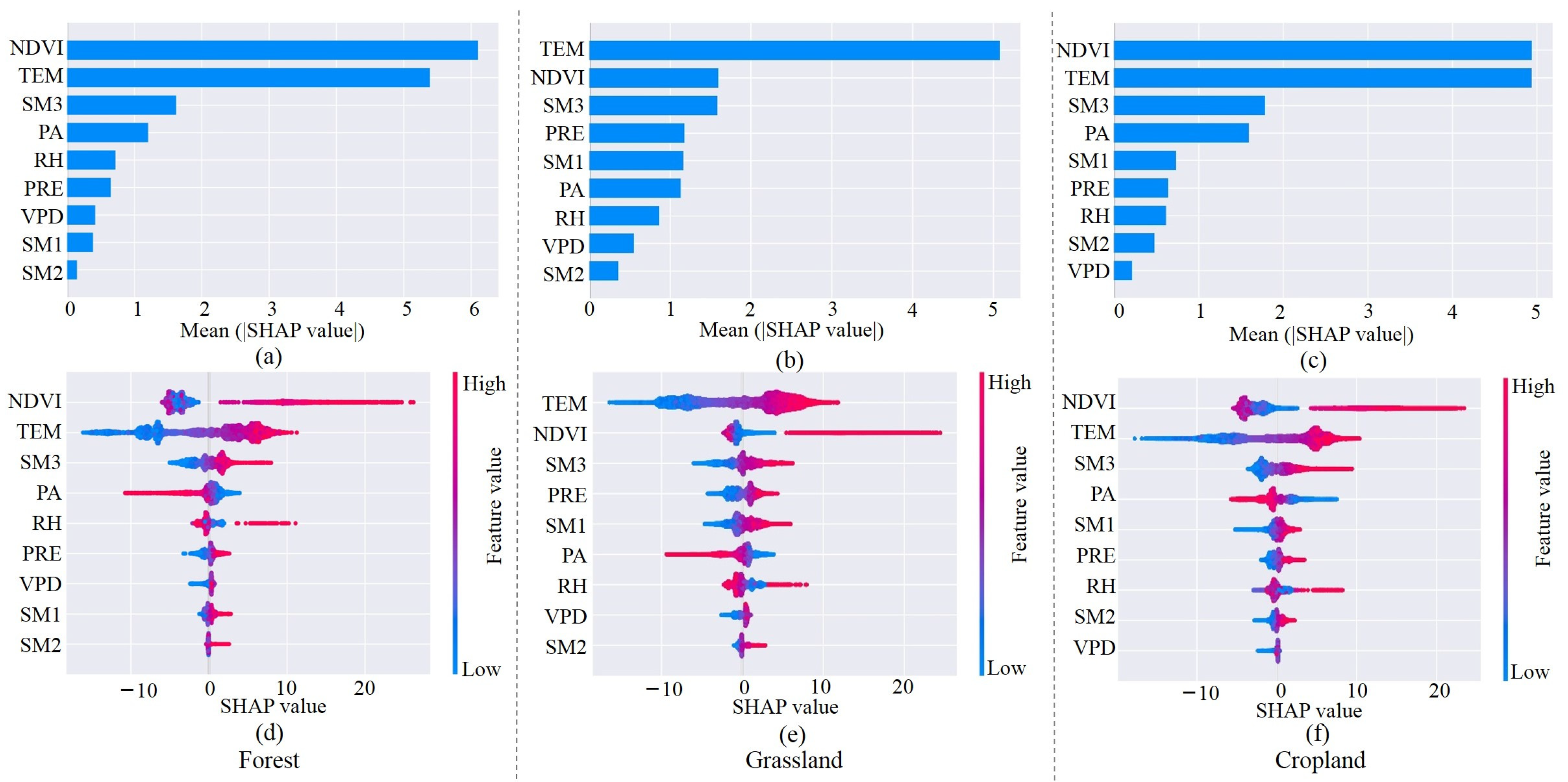
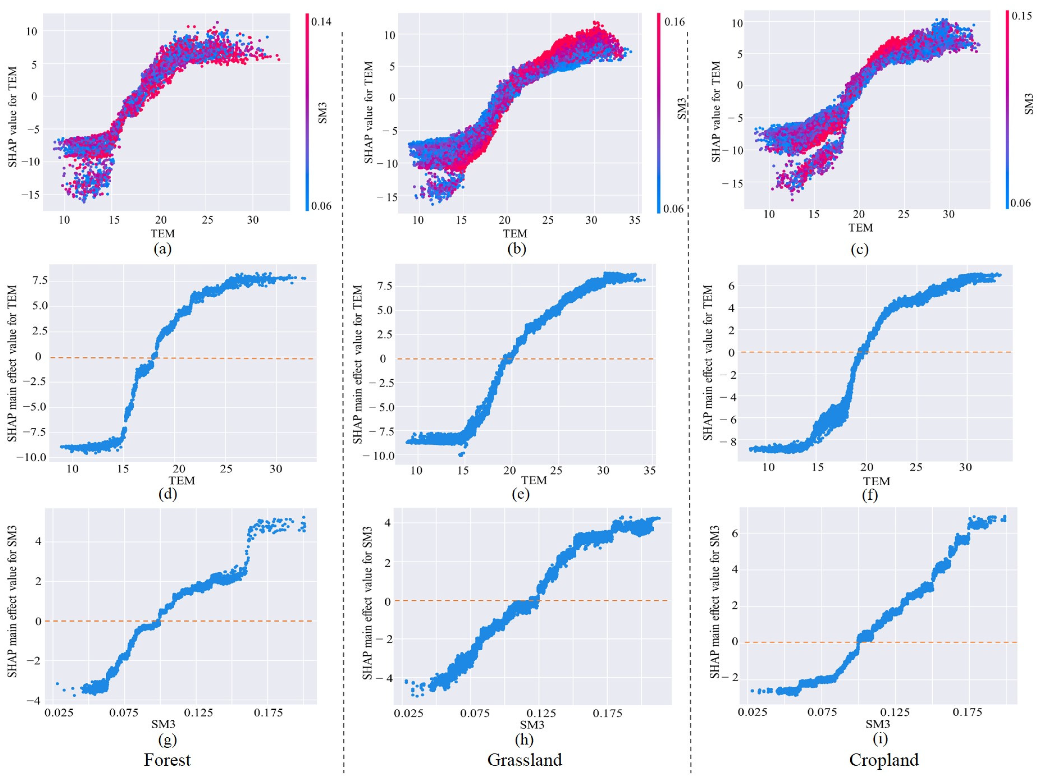
4.2. Drivers of ET Change in Different Plants

Figure 9 shows the SHAP values of each factor contributing to ET–XGB across different plants. If the SHAP value is negative, it indicates that the specialized variables make a loss of prediction value. Figure 9a–c shows that NDVI, TEM, and SM3 were the main factors for ET sensitivities in the forest, grassland, and cropland. PA and RH were the secondary factors in the woods, PRE and SM1 were the secondary factors on grassland and PA, and SM1 was the secondary factor on cropland for ET sensitivities. Compared with precipitation, the temperature was the main climate factor for ET on these three plants. The maximum NDVI SHAP values in forests are 6.1 W/m², and the minimum NDVI SHAP values in grasslands are 1.6 W/m². Because the range span is large, it shows that the change in NDVI can significantly affect ET.

Moreover, to the right of the 0-value line, the SHAP values gradually increased with increasing NDVI, indicating a significant positive correlation between NDVI and evapotranspiration (Figure 9d–f). The SHAP values of TEM in all three sub-bedding cases are about 5 W/m², while the SHAP values of TEM in Figure 9d–f are also uniformly distributed around the value of 0. Additionally, there is an apparent aggregation state within a certain temperature value, which indicates that either too high or too low temperature will initiate the main effect on ET and further confirms that there is a threshold effect of temperature on ET. Although the soil moisture in the root zone (SM3) was the main factor for ET sensitivities, the SHAP values of SM3 showed a relatively aggregative state under around the value of 0, no matter in forest or grassland (Figure 9d–f). This indicates that ET is low when the soil water content is small. For cropland, the left tails of SHAP values are very scattered, indicating the more significant the soil moisture content in the root zone, the greater the ET. Other climate factors limited the average contribution of VPD (0.3 W/m²) to ET–XGB. However, if VPD is low, it will also inhibit the ET of plants (Figure 9d–f). Except for air pressure, other factors have positive effects on ET. In summary, the TEM and NDVI are the relatively critical driving factors for the ET of different plants. Compared with VPD, soil moisture is dominant for plant water stress in arid and semi-arid regions. To further understand whether and how the three main factors affect each other, we use the shape correlation diagram from the SHAP package to explore.

4.3. Coupling Effect and Threshold Effect of Temperature and Soil Moisture on ET Dynamics

The SHAP dependence plot can explain the given variables and how to affect the prediction of each sample. At the same time, it can also be used to judge whether there is a coupling effect between different influencing factors. Therefore, the SHAP dependence plots were used to explore the coupling effect between these three main factors. Human activities have greatly disturbed vegetation restoration after 2000, so we mainly analyze the coupling effect of temperature and soil moisture on ET dynamics.

Figure 10a–c shows that TEM and SM3 have a noticeable coupling effect. Specifically, the slope of the SHAP value is positive, and a high TEM was usually coupled with a higher SM3, producing positive SHAP values. However, the coupling effect in grassland is more vital than in forests and cropland. Compared with Figure 10a,c, when TEM is the same, with the increase in SM3, the SHAP value in grassland increased more obviously, which suggests that a high root zone soil moisture can bring a higher ET loss in arid and semi-arid regions. In contrast, due to the influence of human irrigation activities, the coupling effect between farmland and woodland is not very prominent.

The SHAP main effect value of TEM always increased with increasing TEM (Figure 10d–f), indicating that the positive effect of TEM on ET increased. The SHAP main values become flattened when the temperature value is over 25, 30, and 30 °C in the forest, grassland, and cropland. Therefore, the threshold values are 25, 30, and 30 °C in the forest, grassland, and cropland, respectively. However, the threshold effect of SM3 is less obvious, the SHAP main effect value of SM3 always increased with increasing SM3 (Figure 10g–i). In forests and croplands, when the SM3 exceeded 0.1 m³/m³, the influence of SM3 on ET was positive. In grasslands, when the SM3 exceeded 0.125 m³/m³, the influence of SM3 on ET was positive. A threshold of TEM on ET was identified in the study area, once the threshold is exceeded, the increase in temperature will not lead to the growth of ET. When the temperature rises to a certain value, the plant will choose to close its pores to sustain water in the leaves and stop transpiration. Therefore, the main cause of vegetation ET affecting the study area is heat.

Although we found the primary factors and the threshold effect of ET in different plants, this study also has some uncertainties. First, in this study, we only considered the response relationship between climate change and vegetation ET on a monthly scale. Second, this study did not consider the irrigation and managements measures over croplands. Therefore, future studies should consider the impacts of climate change and human activities on vegetation ET at various time scales.

5. Conclusions

The accurate simulation of actual ET has always been necessary for scientific research. This study used an improved new PT-JPL model to obtain the actual ET in the study area. We compared the simulation data over the Inner Mongolia Reach of the Yellow River Basin area with remotely sensed ET products and eddy-covariance data. In addition, the extreme gradient boosting models–Shapley additive explanations framework were used to identify the primary factors and their threshold effect for ET in different plants.

The main findings were as follows:

1. The results of the eddy-covariance flux tower and PML-V2 data sets show that the new PT-JPL model, which incorporates soil moisture constraints on evaporation and transpiration simulation, can accurately simulate the spatiotemporal variation of actual evapotranspiration in the study area.

2. Soil evaporation is the main part of the actual ET increase in the study area. Implementing ecological restoration projects reduced the exposed land area in the study area and reduced the rate of total LE effectively. After 1999, the increase rate of LE reduced from 0.068 W/m² to 0.009 W/m², and the increase rate of LE_s reduced from 0.012 W/m² to −0.021 W/m².

3. Since the ecological restoration project was implemented in 1999 by the Chinese government, the ET of forests and grasslands has decreased in the growing season. On the contrary, cropland ET is increasing yearly, while the cropland area has not increased significantly. Therefore, it is necessary to adjust the planting structure and irrigation methods to save water and reduce ET effectively.

4. NDVI, temperature and root zone soil moisture were the main environmental factors causing ET changes in different plants. Meanwhile, temperature and root zone soil moisture have a noticeable coupling effect, except grassland. Additionally, there was a pronounced threshold effect of temperature stress on ET, which is 25, 30, and 30 °C in the forest, grassland, and cropland.

References

1. Yi, Y.H.; Yang, D.W.; Liu, Y.; Xu, D. Review of study on regional evapotranspiration modeling on remote sensing. Shui Li Xue Bao 2008, 39, 7. [Google Scholar]
2. Liu, X.M.; Zheng, H.X.; Liu, C.M.; Cao, Y.J. Sensitivity of the Potential Evapotranspiration to Key Climatic Variables in the Haihe River Basin. Resour. Sci. 2009, 31, 1470–1476. [Google Scholar]
3. Qiang, L.; Yang, Z. Quantitative estimation of the impact of climate change on actual evapotranspiration in the Yellow River Basin, China. J. Hydrol. 2010, 395, 226–234. [Google Scholar]
4. Sun, G.; Alstad, K.; Chen, J.; Chen, S.P.; Ford, C.R.; Lin, G.H.; Liu, C.F.; Lu, N.; McNulty, S.G.; Miao, H.X.; et al. A general predictive model for estimating monthly ecosystem evapotranspiration. Ecohydrology 2011, 4, 245–255. [Google Scholar] [CrossRef]
5. Xia, J.Z.; Liang, S.L.; Chen, J.Q.; Yuan, W.P.; Liu, S.G.; Li, L.H.; Cai, W.W.; Zhang, L.; Fu, Y.; Zhao, T.B.; et al. Satellite-Based Analysis of Evapotranspiration and Water Balance in the Grassland Ecosystems of Dryland East Asia. PLoS ONE 2014, 9, e97295. [Google Scholar] [CrossRef]
6. Xue, B.; A, Y.; Wang, G.; Helman, D.; Sun, G.; Tao, S.; Liu, T.; Yan, D.; Zhao, T.; Zhang, H.; et al. Divergent Hydrological Responses to Forest Expansion in Dry and Wet Basins of China: Implications for Future Afforestation Planning. Water Resour. Res. 2022, 5, e2021WR031856. [Google Scholar] [CrossRef]
7. Xue, B.L.; Helman, D.; Wang, G.Q.; Xu, C.Y.; Xiao, J.F.; Liu, T.X.; Wang, L.; Li, X.P.; Duan, L.M.; Lei, H.M. The low hydrologic resilience of Asian Water Tower basins to adverse climatic changes. Adv. Water Resour. 2021, 155, 103996. [Google Scholar] [CrossRef]
8. Valipour, M. Study of different climatic conditions to assess the role of solar radiation in reference crop evapotranspiration equations. Arch. Acker Pfl. Boden 2015, 61, 679–694. [Google Scholar] [CrossRef]
9. Falamarzi, Y.; Palizdan, N.; Huang, Y.F.; Lee, T.S. Estimating evapotranspiration from temperature and wind speed data using artificial and wavelet neural networks (WNNs). Agric. Water Manag. 2014, 140, 26–36. [Google Scholar] [CrossRef]
10. Allen, R.G.; Pereira, L.S.; Raes, D.; Smith, M. Crop Evapotranspiration-Guidelines for Computing Crop Water Requirements-FAO Irrigation and Drainage Paper 56; FAO: Rome, Italy, 1998; Volume 300, p. D05109. [Google Scholar]
11. Martens, S.N.; Breshears, D.D.; Meyer, C.W. Spatial distributions of understory light along the grassland/forest continuum: Effects of cover, height, and spatial pattern of tree canopies. Ecol. Model. 2000, 126, 79–93. [Google Scholar] [CrossRef]
12. Panferov, O.; Knyazikhin, Y.; Myneni, R.B.; Szarzynski, J.; Engwald, S.; Schnitzler, K.G.; Gravenhorst, G. The role of canopy structure in the spectral variation of transmission and absorption of solar radiation in vegetation canopies. IEEE Trans. Geosci. Remote 2001, 39, 241–253. [Google Scholar] [CrossRef]
13. Lv, Y.Z.; Hu, K.L.; Li, B.G. The spatio-temporal variability of soil water in sand dunes in maowusu desert. Acta Pedol. Sin. 2006, 43, 152–154. (In Chinese) [Google Scholar]
14. Zeng, N.; Yoon, J. Expansion of the world’s deserts due to vegetation-albedo feedback under global warming. Geophys. Res. Lett. 2009, 36, L17401. [Google Scholar] [CrossRef]
15. Maayar, M.; Chen, J.M. Spatial scaling of evapotranspiration as affected by heterogeneities in vegetation, topography, and soil texture. Remote Sens. Environ. 2006, 102, 33–51. [Google Scholar] [CrossRef]
16. Wang, Y.H. The hydrological influence of black locust plantations in the loess area of northwest China. Hydrol. Process. 1992, 6, 241–251. [Google Scholar]
17. Liu, J.G.; Li, S.X.; Ouyang, Z.Y.; Tam, C.; Chen, X.D. Ecological and socioeconomic effects of China’s policies for ecosystem services. Proc. Natl. Acad. Sci. USA 2008, 105, 9477–9482. [Google Scholar] [CrossRef] [PubMed]
18. Fu, B.J.; Chen, L.D. Agricultural landscape spatial pattern analysis in the semi-arid hill area of the Loess Plateau, China. J. Arid Environ. 2000, 44, 291–303. [Google Scholar] [CrossRef]
19. Wang, C.; Zhen, L.; Du, B.Z.; Sun, C.Z. Assessment of the impact of Grain for Green project on farmers’ livelihood in the Loess Plateau. Chin. J. Eco-Agric. 2014, 22, 850–858. [Google Scholar]
20. Fu, B.J.; Yu, L.; Lü, Y.H.; He, C.S.; Zeng, Y.; Wu, B.F. Assessing the soil erosion control service of ecosystems change in the Loess Plateau of China. Ecol. Complex. 2011, 8, 284–293. [Google Scholar] [CrossRef]
21. Jia, X.Q.; Fu, B.J.; Feng, X.M.; Hou, G.H.; Liu, Y.; Wang, X.F. The tradeoff and synergy between ecosystem services in the Grainfor Green areas in Northern Shaanxi, China. Ecol. Indic. 2014, 43, 103. [Google Scholar] [CrossRef]
22. Feng, X.M.; Fu, B.J.; Piao, S.L.; Wang, S.; Ciais, P.; Zeng, Z.Z.; Lü, Y.H.; Li, Y.; Jiang, X.H.; Wu, B.; et al. Revegetation in China’s Loess Plateau is approaching sustainable water resource limits. Nat. Clim. Chang. 2016, 6, 1019–1022. [Google Scholar] [CrossRef]
23. Li, S.; Liang, W.; Fu, B.J.; Lü, Y.H.; Fu, S.Y.; Wang, S.; Su, H.M. Vegetation changes in recent large-scale ecological restoration projects and subsequent impact on water resources in China’s Loess Plateau. Sci. Total Environ. 2016, 569, 1032–1039. [Google Scholar] [CrossRef] [PubMed]
24. Liu, Y.B.; Xiao, J.F.; Ju, W.M.; Xu, K.; Zhou, Y.L.; Zhao, Y.T. Recent trends in vegetation greenness in China significantly altered annual evapotranspiration and water yield. Environ. Res. Lett. 2016, 11, 0940109. [Google Scholar] [CrossRef]
25. Zhao, G.J.; Kondolf, G.M.; Mu, X.M.; Han, M.W.; He, Z.; Rubin, Z.; Wang, F.; Gao, P.; Sun, W.Y. Sediment yield reduction associated with land use changes and check dams in a catchment of the Loess Plateau, China. Catena 2017, 148, 126–137. [Google Scholar] [CrossRef]
26. Gao, P.; Deng, J.C.; Chai, X.K.; Mu, X.M.; Zhao, G.J.; Shao, H.B.; Sun, W.Y. Dynamic sediment discharge in the Hekou-Longmen region of Yellow River and soil and water conservation implications. Sci. Total Environ. 2017, 578, 56–66. [Google Scholar] [CrossRef] [PubMed]
27. Peng, S.S.; Piao, S.L.; Zeng, Z.Z.; Ciais, P.; Zhou, L.M.; Li, L.Z.X.; Myneni, R.B.; Yin, Y.; Zeng, H. Afforestation in China cools local land surface temperature. Proc. Natl. Acad. Sci. USA 2014, 111, 2915. [Google Scholar] [CrossRef] [Green Version]
28. Arora, V.K.; Montenegro, A. Small temperature benefits provided by realistic afforestation efforts. Nat. Geosci. 2011, 4, 514–518. [Google Scholar] [CrossRef]
29. Yao, Y.; Liang, S.; Cheng, J.; Liu, S.; Fisher, J.B.; Zhang, X.; Jia, K.; Zhao, X.; Qin, Q.; Zhao, B. MODIS-driven estimation of terrestrial latent heat flux in China based on a modified Priestley–Taylor algorithm. Agric. For. Meteorol. 2013, 171, 187–202. [Google Scholar] [CrossRef]
30. Detto, M.; Montaldo, N.; Albertson, J.D.; Mancini, M.; Katul, G. Soil moisture and vegetation controls on evapotranspiration in a heterogeneous Mediterranean ecosystem on Sardinia, Italy. Water Resour. Res. 2006, 422, 356–367. [Google Scholar] [CrossRef]
31. Gao, G.; Chen, D.L.; Xu, C.Y.; Simelton, E. Trend of estimated actual evapotranspiration over China during 1960–2002. J. Geophys. Res. 2007, 112, 1120–1128. [Google Scholar] [CrossRef]
32. Bastiaanssen, W. SEBAL-based sensible and latent heat fluxes in the irrigated Gediz Basin, Turkey. J. Hydrol. 2000, 229, 87–100. [Google Scholar] [CrossRef]
33. Yang, Y.; Shang, S.; Lei, J. Remote sensing temporal and spatial patterns of evapotranspiration and the responses to water management in a large irrigation district of North China. Agric. For. Meteorol. 2012, 164, 112–122. [Google Scholar] [CrossRef]
34. Yang, Y.T.; Long, D.; Guan, H.; Liang, W.; Simmons, C.T.; Batelaan, O. Comparison of three dual-source remote sensing evapotranspiration models during the MUSOEXE-12 campaign: Revisit of model physics. Water Resour. Res. 2015, 51, 3145–3165. [Google Scholar] [CrossRef]
35. Fisher, J.B.; Tu, K.P.; Baldocchi, D.D. Global estimates of the land–atmosphere water flux based on monthly AVHRR and ISLSCP-II data, validated at 16 FLUXNET sites. Remote Sens. Environ. 2008, 112, 901–919. [Google Scholar] [CrossRef]
36. Su, Z. The Surface Energy Balance System (SEBS) for estimation of turbulent heat fluxes. Hydrol. Earth Syst. Sci. 2002, 6, 85–100. [Google Scholar] [CrossRef]
37. Long, D.; Singh, V.P. A Two-source Trapezoid Model for Evapotranspiration (TTME) from satellite imagery. Remote Sens. Environ. 2012, 121, 370–388. [Google Scholar] [CrossRef]
38. Wang, K.; Dickinson, R.E. A review of global terrestrial evapotranspiration: Ob-servation. Rev. Geophys. 2012, 50, RG2005. [Google Scholar]
39. Purdy, A.J.; Fisher, J.B.; Goulden, M.L.; Colliander, A.; Halverson, G.; Tu, K.; Famiglietti, J.S. SMAP soil moisture improves global evapotranspiration. Remote Sens. Environ. 2018, 219, 1–14. [Google Scholar] [CrossRef]
40. Lundberg, S.M.; Erion, G.; Chen, H.; DeGrave, A.; Prutkin, J.M.; Nair, B.G.; Katz, R.; Himmelfarb, J.; Bansal, N.; Lee, S. From Local Explanations to Global Understanding with Explainable AI for Trees. Nat. Mach. Intell. 2020, 2, 56–67. [Google Scholar] [CrossRef]
41. Khosravi, K.; Pham, B.T.; Chapi, K.; Shirzadi, A.; Shahabi, H.; Revhaug, I.; Prakash, I.; Bui, D.T. A comparative assessment of decision trees algorithms for flash flood susceptibility modeling at Haraz watershed, northern Iran. Sci. Total Environ. 2018, 627, 744–755. [Google Scholar] [CrossRef]
42. Yang, Q.L.; Zhang, H.; Wang, G.Q.; Luo, S.S.; Chen, D.Z.; Peng, W.S.; Shao, J.M. Dynamic runoff simulation in a changing environment: A data stream approach. Environ. Modell. Softw. 2018, 112, 157–165. [Google Scholar] [CrossRef]
43. Budholiya, K.; Shrivastava, S.K.; Sharma, V. An optimized XGBoost based diagnostic system for effective prediction of heart disease. J. King Saud Univ. Comput. Inf. Sci. 2020, 34, 4514–4523. [Google Scholar] [CrossRef]
44. Ji, S.W.; Wang, X.J.; Zhao, W.P.; Guo, D. An Application of a Three-Stage XGBoost-Based Model to Sales Forecasting of a Cross-Border E-Commerce Enterprise. Math. Probl. Eng. 2019, 2019, 1–15. [Google Scholar] [CrossRef]
45. Liu, J.Y.; Liu, M.L.; Zhuang, D.F.; Zhang, Z.X.; Deng, X.Z. Study on spatial pattern of land-use change in China during 1995–2000. Sci. China Ser. D-Earth Sci. 2003, 46, 373–384. [Google Scholar]
46. Liu, J.Y.; Zhang, Z.X.; Zhuang, D.F.; Wang, Y.M.; Zhou, W.C.; Zhang, S.W.; Li, R.D.; Jiang, N.; Wu, S.X. A study on the spatial-temporal dynamic changes of land- use and driving forces analyses of China in the 1990s. Geogr. Res. 2003, 22, 1–12. [Google Scholar]
47. Liu, J.Y.; Zhang, Z.X.; Xu, X.L.; Kuang, W.H.; Zhou, W.C.; Zhang, S.W.; Li, R.D.; Yan, C.Z.; Yu, D.S.; Wu, S.X.; et al. Spatial patterns and driving forces of land use change in China during the early 21st century. J. Geogr. Sci. 2010, 20, 483–494. [Google Scholar] [CrossRef]
48. Liu, J.Y.; Kuang, W.H.; Zhang, Z.X.; Xu, X.L.; Qin, Y.W.; Ning, J.; Zhou, W.C.; Zhang, S.W.; Li, R.D.; Yan, C.Z.; et al. Spatiotemporal characteristics, patterns, and causes of land-use changes in China since the late 1980s. J. Geogr. Sci. 2014, 24, 195–210. [Google Scholar] [CrossRef]
49. Zhang, Y.Q.; Kong, D.D.; Gan, R.; Chiew, F.H.S.; McVicar, T.; Zhang, Q.; Yang, Y.T. Coupled estimation of 500 m and 8-day resolution global evapotranspiration and gross primary production in 2002–2017. Remote Sens. Environ. 2019, 222, 165–182. [Google Scholar] [CrossRef]
50. Priestley, C.; Taylor, R.J. On the Assessment of Surface Heat Flux and Evaporation Using Large Scale Parameters. Mon. Weather Rev. 1972, 100, 81–92. [Google Scholar] [CrossRef]
51. Wang, G.Q.; Zhang, X.J.; Yinglan, A.; Duan, L.M.; Xue, B.l.; Liu, T.X. A Spatio-temporal Cross Comparison Framework for the Accuracies of Remotely Sensed Soil Moisture Products in a Climate-Sensitive Grassland Region. J. Hydrol. 2021, 597, 126089. [Google Scholar] [CrossRef]
52. Chen, T.; Guestrin, C. XGBoost: A Scalable Tree Boosting System. In Proceedings of the 22nd ACM SIGKDD International Conference, San Francisco, CA, USA, 13–17 August 2016; ACM: New York, NY, USA, 2016. [Google Scholar]
53. Meng, Y.; Yang, N.; Qian, Z.; Zhang, G. What makes an online review more helpful: An interpretation framework using XGBoost and SHAP values. J. Theor. Appl. Electron. Commer. Res. 2021, 16, 466–490. [Google Scholar] [CrossRef]
54. Adadi, A.; Berrada, M. Peeking inside the black-box: A survey on explainable artificial intelligence. IEEE Access 2018, 6, 52138–52160. [Google Scholar] [CrossRef]
55. Rudin, C. Stop explaining black box machine learning models for high stakes decisions and use interpretable models instead. Nat. Mach. Intell. 2019, 1, 206–215. [Google Scholar] [CrossRef] [PubMed]
56. Feng, D.C.; Wang, W.J.; Mangalathu, S.; Taciroglu, E. Interpretable XGBoost-SHAP machine- learning model for shear strength prediction of Squat RC walls. J. Struct. Eng. 2021, 147, 04021173. [Google Scholar] [CrossRef]
57. Guo, M.Z.; Yuan, Z.Z.; Janson, B.; Peng, Y.X.; Yang, Y.; Wang, W.C. Older Pedestrian Traffic Crashes Severity Analysis Based on an Emerging Machine Learning XGBoost. Sustainability 2021, 13, 926. [Google Scholar] [CrossRef]
58. Yang, J.M.; Yao, Y.J.; Shao, C.L.; Li, Y.F.; Fisher, J.B.; Chen, J.; Chen, J.Q.; Jia, K.; Zhang, X.T.; Shang, K.; et al. A novel TIR-derived three-source energy balance model for estimating daily latent heat flux in mainland China using an all-weather land surface temperature product. Agric. For. Meteorol. 2022, 323, 109066. [Google Scholar] [CrossRef]
59. Michel, D.; Jiménez, C.; Miralles, D.G.; Jung, M.; Hirschi, M.; Ershadi, A.; Martens, B.; McCabe, M.F.; Fisher, J.B.; Mu, Q.Z.; et al. The WACMOS-ET project—Part 1: Tower-scale evaluation of four remote-sensing-based evapotranspiration algorithms. Hydrol. Earth Syst. Sci. 2016, 20, 803–822. [Google Scholar] [CrossRef] [Green Version]
Figure 1. Research framework.
Remotesensing 14 04499 g001
Figure 2. Location of the Inner Mongolia Reach of the Yellow River Basin; the land use/cover map is from 2015.
Remotesensing 14 04499 g002
Figure 3. (a) Change in the area of different land use in the Inner Mongolia Reach of the Yellow River Basin from 1990 to 2015, and (b) transfer direction between the different land use in the Inner Mongolia Reach of the Yellow River Basin from 1990 to 2015.
Remotesensing 14 04499 g003
Figure 4. Compared accuracy of the original (PT-JPL) and improved model (new PT-JPL) against eddy-covariance flux tower latent heat data from 1 January 2006 to 30 September 2009 in the study area. (a,b) Comparison results of site KBQ04, and (c,d) comparison results of site KBQ05.
Remotesensing 14 04499 g004
Figure 5. Spatial distribution of the correlation coefficient of the performance of the improved models (new PT-JPL) against the PML-V2 evapotranspiration data from 1 January 2006 to 30 September 2009 in the study area. (a) Vegetation canopy transpiration, E c ; (b) soil evaporation, E s ; (c) vegetation canopy interception evaporation, E i .
Remotesensing 14 04499 g005
Figure 6. The spatial distribution of multiyear-averaged latent heat values during the 1982–2015 period in the study area: (a) total actual L E ; (b) vegetation canopy transpiration, L E c ; (c) soil evaporation, L E s ; (d) vegetation canopy interception evaporation, L E i .
Remotesensing 14 04499 g006
Figure 7. The time series of multiyear latent heat values during the 1982–2015 period in the study area: the time variation of (a) total actual L E ; (b) vegetation canopy transpiration, L E c ; (c) soil evaporation, L E s .
Remotesensing 14 04499 g007
Figure 8. The time series of multiyear ET values during the 2000–2015 period on different land use in the growing season.
Remotesensing 14 04499 g008
Figure 9. SHAP value of different factors. (ac) Bar plot of the mean absolute SHAP values affecting ET on different plant. (df) A set of bee swarm plots in forest, grassland, and cropland. The SHAP value mean influence of variables on ET–XGB model prediction of this sample.
Remotesensing 14 04499 g009
Figure 10. Identification of the SHAP main effect and coupling effect of temperature (TEM) and root zone soil moisture (SM3) on ET. (ac) SHAP dependence plot of TEM versus its SHAP value along SM3. (df) SHAP main effect value for TEM on ET. (gi) SHAP main effect value for SM3 on ET.
Remotesensing 14 04499 g010