

Quantifying Basal Roughness and Internal Layer Continuity Index of Ice Sheets by an Integrated Means with Radar Data and Deep Learning


Abstract
:
1. Introduction
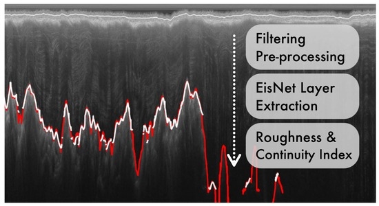
2. Method
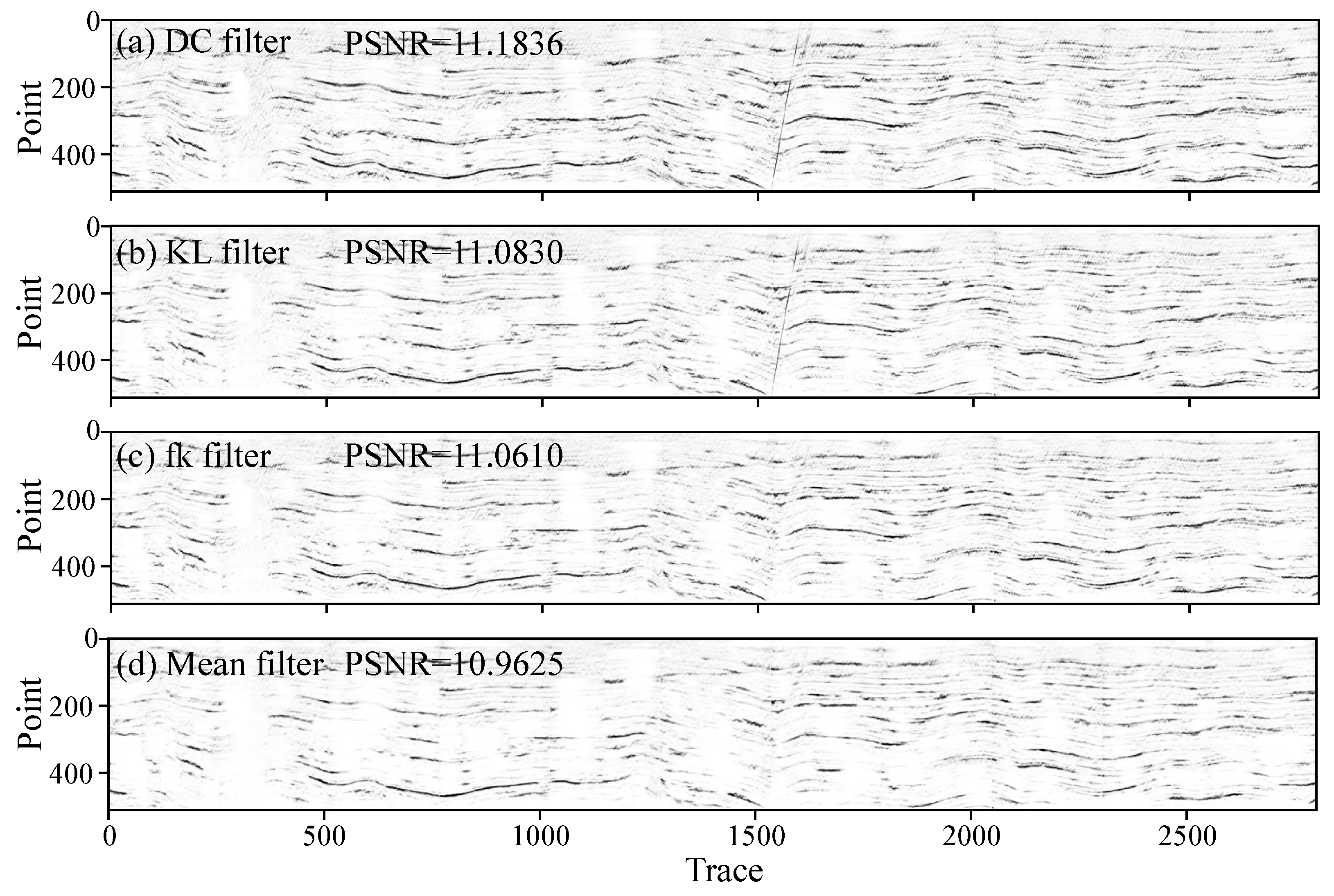
2.1. Geophysics Preprocessing
2.2. EisNet Model
2.3. Basal Roughness
2.4. Internal Layer Continuity Index
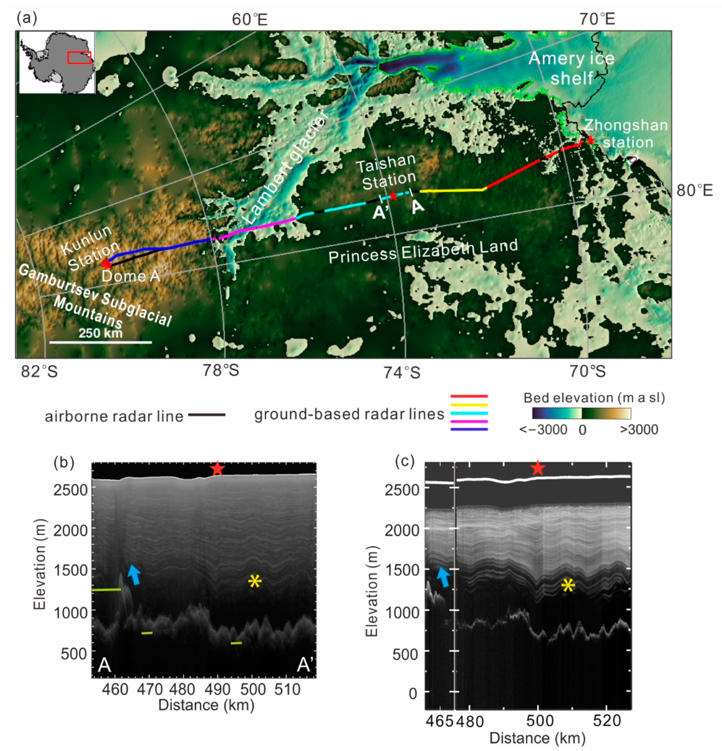
3. Test Ice Sheet Profile and Radar Data
4. Results and Discussion
4.1. Radar Detection
4.2. Bedrock Interface and Internal Ice Layer Extraction
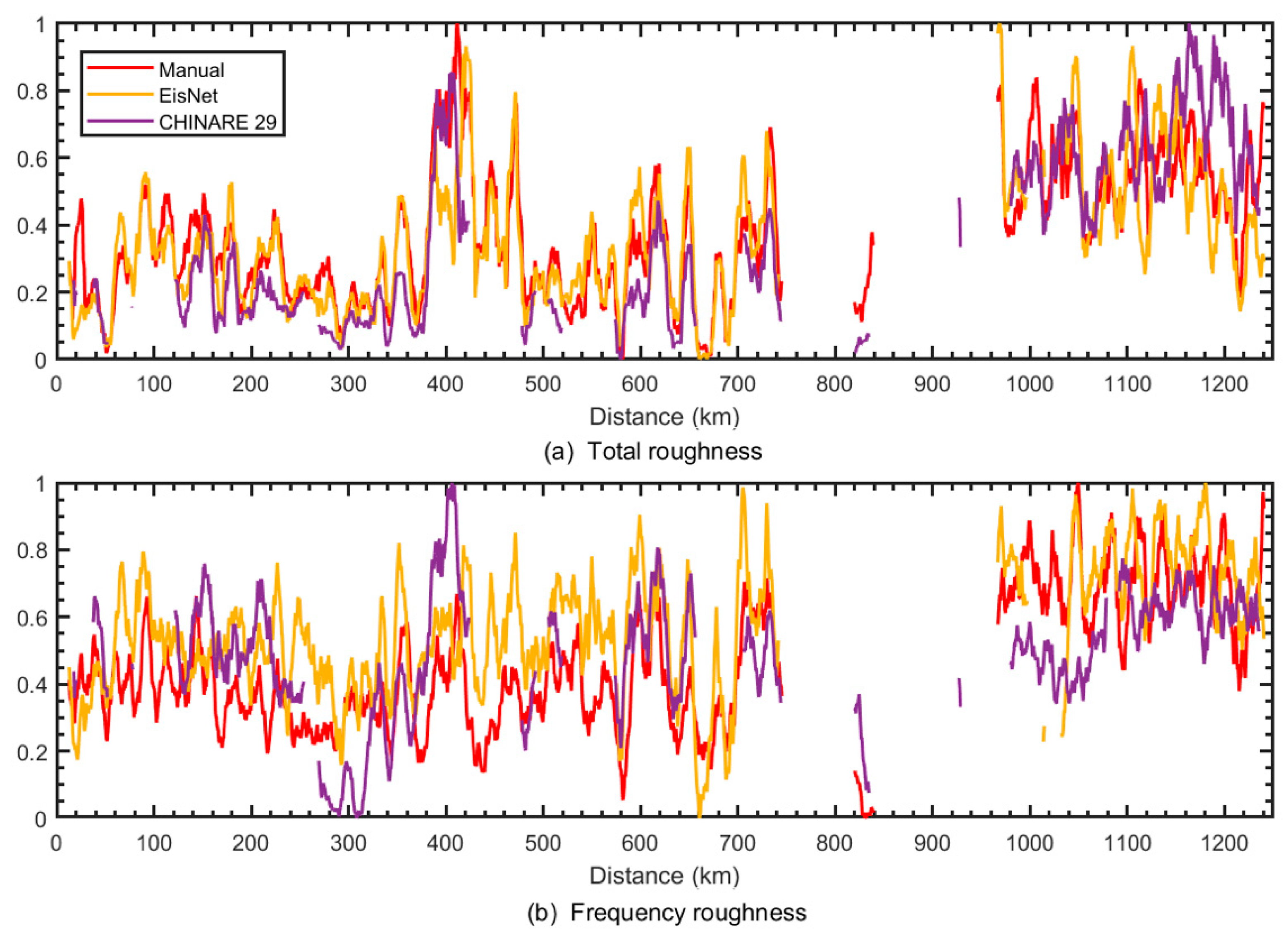
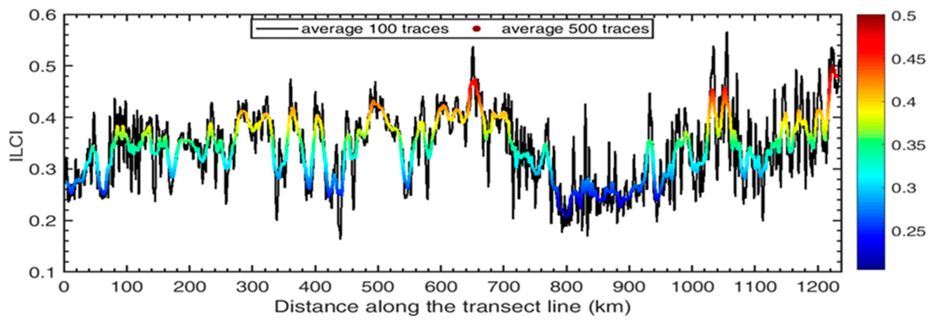
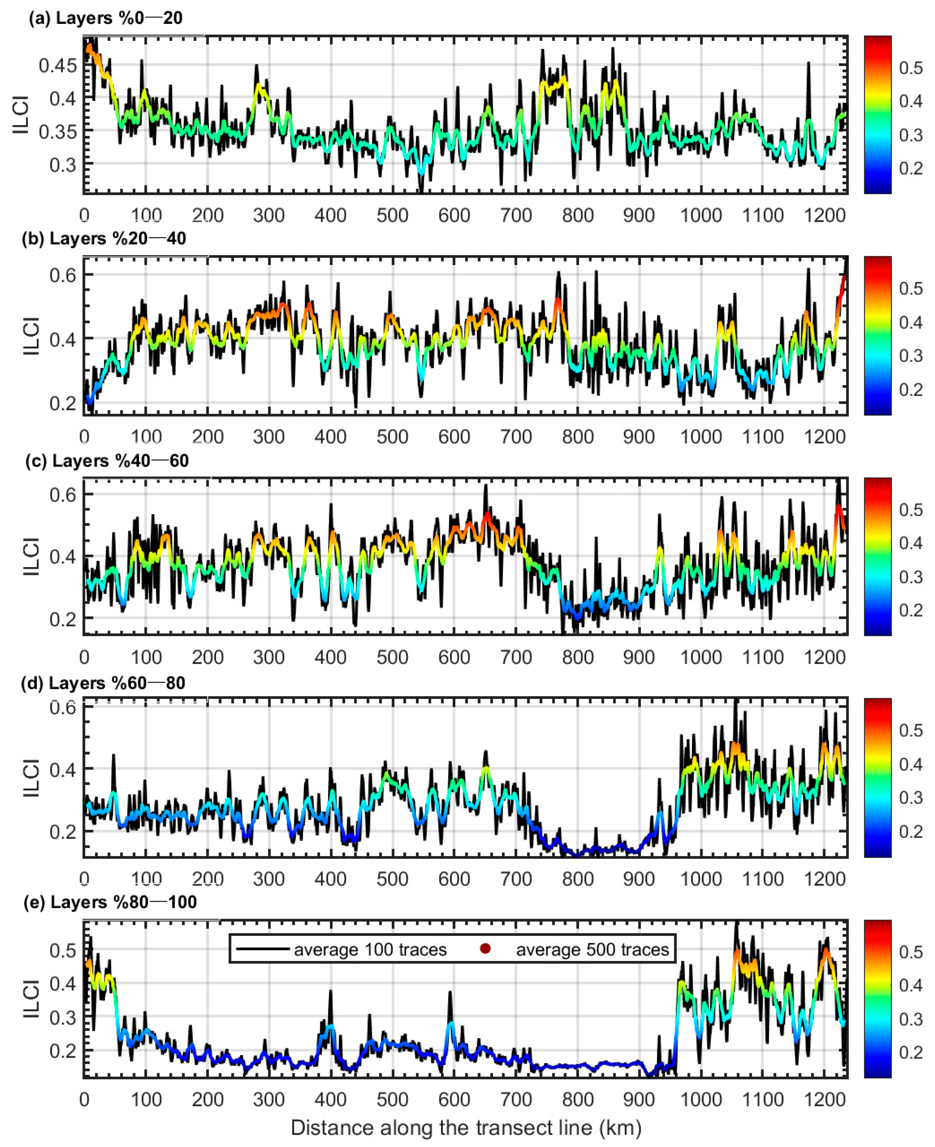
4.3. Basal Roughness and Continuity Index
4.4. Discussion
5. Conclusions
Author Contributions
Funding
Acknowledgments
Conflicts of Interest
References
- IPCC. Climate Change 2021: The Physical Science Basis. Available online: https://www.ipcc.ch/report/ar6/wg1/downloads/report/IPCC_AR6_WGI_Full_Report.pdf (accessed on 1 August 2021).
- Frederikse, T.; Buchanan, M.K.; Lambert, E.; Kopp, R.E.; Oppenheimer, M.; Rasmussen, D.; van de Wal, R.S. Antarctic Ice Sheet and emission scenario controls on 21st-century extreme sea-level changes. Nat. Commun. 2020, 11, 1–11. [Google Scholar] [CrossRef] [PubMed]
- Golledge, N.R.; Kowalewski, D.E.; Naish, T.R.; Levy, R.H.; Fogwill, C.J.; Gasson, E.G. The multi-millennial Antarctic commitment to future sea-level rise. Nature 2015, 526, 421–425. [Google Scholar] [CrossRef] [PubMed]
- Pattyn, F. The paradigm shift in Antarctic ice sheet modelling. Nat. Commun. 2018, 9, 1–3. [Google Scholar] [CrossRef]
- Deconto, R.M.; Pollard, D. Contribution of Antarctica to past and future sea-level rise. Nature 2016, 531, 591–597. [Google Scholar] [CrossRef]
- Graham, F.S.; Roberts, J.L.; Galton-Fenzi, B.K.; Young, D.; Blankenship, D.; Siegert, M.J. A high-resolution synthetic bed elevation grid of the Antarctic continent. Earth Syst. Sci. Data 2017, 9, 267–279. [Google Scholar] [CrossRef]
- McCormack, F.S.; Roberts, J.L.; Jong, L.M.; Young, D.A.; Beem, L.H. A note on digital elevation model smoothing and driving stresses. Polar Res. 2019, 38. [Google Scholar] [CrossRef]
- Fretwell, P.; Pritchard, H.D.; Vaughan, D.G.; Bamber, J.L.; Barrand, N.E.; Bell, R.; Bianchi, C.; Bingham, R.; Blankenship, D.D.; Casassa, G. Bedmap2: Improved ice bed, surface and thickness datasets for Antarctica. Cryosphere 2013, 7, 375–393. [Google Scholar] [CrossRef]
- Morlighem, M.; Rignot, E.; Binder, T.; Blankenship, D.; Drews, R.; Eagles, G.; Eisen, O.; Ferraccioli, F.; Forsberg, R.; Fretwell, P. Deep glacial troughs and stabilizing ridges unveiled beneath the margins of the Antarctic ice sheet. Nat. Geosci. 2020, 13, 132–137. [Google Scholar] [CrossRef]
- Edwards, T.L.; Nowicki, S.; Marzeion, B.; Hock, R.; Zwinger, T. Projected land ice contributions to twenty-first-century sea level rise. Nature 2021, 593, 74–82. [Google Scholar] [CrossRef]
- Sutter, J.; Fischer, H.; Eisen, O. Investigating the internal structure of the Antarctic ice sheet: The utility of isochrones for spatiotemporal ice-sheet model calibration. Cryosphere 2021, 15, 3839–3860. [Google Scholar] [CrossRef]
- Bogorodsky, V.V.E.; Bogorodskiĭ, V.V.E.; Bentley, C.R.; Gudmandsen, P. Radioglaciology; Reidel, D., Ed.; Springer Science & Business Media: Dordrecht, The Netherlands, 1985; Volume 1. [Google Scholar]
- Chu, W.; Hilger, A.M.; Culberg, R.; Schroeder, D.M.; Jordan, T.M.; Seroussi, H.; Young, D.A.; Blankenship, D.D.; Vaughan, D.G. Multisystem synthesis of radar sounding observations of the Amundsen Sea sector from the 2004–2005 field season. J. Geophys. Res. Earth Surf. 2021, 126, e2021JF006296. [Google Scholar] [CrossRef] [PubMed]
- Schroeder, D.M.; Bingham, R.G.; Blankenship, D.D.; Christianson, K.; Eisen, O.; Flowers, G.E.; Karlsson, N.B.; Koutnik, M.R.; Paden, J.D.; Siegert, M.J. Five decades of radioglaciology. Ann. Glaciol. 2020, 61, 1–13. [Google Scholar] [CrossRef]
- Schroeder, D.M.; Dowdeswell, J.A.; Siegert, M.J.; Bingham, R.G.; Chu, W.; MacKie, E.J.; Siegfried, M.R.; Vega, K.I.; Emmons, J.R.; Winstein, K. Multidecadal observations of the Antarctic ice sheet from restored analog radar records. Proc. Natl. Acad. Sci. USA 2019, 116, 18867–18873. [Google Scholar] [CrossRef]
- Tang, X.; Sun, B. Towards an integrated study of subglacial conditions in Princess Elizabeth Land, East Antarctica. Adv. Polar Sci. 2021, 32, 75–77. [Google Scholar]
- Macgregor, J.A.; Boisvert, L.N.; Medley, B.; Petty, A.A.; Yungel, J.K. The scientific legacy of NASA’s Operation IceBridge. Rev. Geophys. 2021, 59, e2020RG000712. [Google Scholar] [CrossRef]
- Frémand, A.C.; Bodart, J.A.; Jordan, T.A.; Ferraccioli, F.; Robinson, C.; Corr, H.F.; Peat, H.J.; Bingham, R.G.; Vaughan, D.G. British Antarctic Survey’s Aerogeophysical Data: Releasing 25 Years of Airborne Gravity, Magnetic, and Radar Datasets over Antarctica. Earth Syst. Sci. Data Discuss. 2022, 14, 1–49. [Google Scholar] [CrossRef]
- Li, X.; Sun, B.; Siegert, M.J.; Bingham, R.G.; Tang, X.; Zhang, D.; Cui, X.; Zhang, X. Characterization of subglacial landscapes by a two-parameter roughness index. J. Glaciol. 2010, 56, 831–836. [Google Scholar] [CrossRef]
- Luo, K.; Liu, S.; Guo, J.; Wang, T.; Li, L.; Cui, X.; Sun, B.; Tang, X. Radar-Derived Internal Structure and Basal Roughness Characterization along a Traverse from Zhongshan Station to Dome A, East Antarctica. Remote Sens. 2020, 12, 1079. [Google Scholar] [CrossRef]
- Jordan, T.M.; Cooper, M.A.; Schroeder, D.M.; Williams, C.N.; Paden, J.D.; Siegert, M.J.; Bamber, J.L. Self-affine subglacial roughness: Consequences for radar scattering and basal water discrimination in northern Greenland. Cryosphere 2017, 11, 1247–1264. [Google Scholar] [CrossRef]
- Schroeder, D.M.; Blankenship, D.D.; Young, D.A. Evidence for a water system transition beneath Thwaites Glacier, West Antarctica. Proc. Natl. Acad. Sci. USA 2013, 110, 12225–12228. [Google Scholar] [CrossRef]
- Siegert, M.J.; Taylor, J.; Payne, A.J. Spectral roughness of subglacial topography and implications for former ice-sheet dynamics in East Antarctica. Global Planet. Chang. 2005, 45, 249–263. [Google Scholar] [CrossRef]
- Taylor, J.; Siegert, M.J.; Payne, A.J.; Hubbard, B. Regional-scale bed roughness beneath ice masses: Measurement and analysis. Comput. Geosci. 2004, 30, 899–908. [Google Scholar] [CrossRef]
- Shepard, M.K.; Campbell, B.A.; Bulmer, M.H.; Farr, T.G.; Gaddis, L.R.; Plaut, J.J. The roughness of natural terrain: A planetary and remote sensing perspective. J. Geophys. Res. Planets 2001, 106, 32777–32795. [Google Scholar] [CrossRef]
- Rippin, D.M.; Bingham, R.G.; Jordan, T.A.; Wright, A.P.; Ross, N.; Corr, H.F.; Ferraccioli, F.; Le Brocq, A.M.; Rose, K.C.; Siegert, M.J. Basal roughness of the Institute and Möller Ice Streams, West Antarctica: Process determination and landscape interpretation. Geomorphology 2014, 214, 139–147. [Google Scholar] [CrossRef]
- Lang, S.; Xu, B.; Cui, X.; Luo, K.; Guo, J.; Tang, X.; Cai, Y.; Sun, B.; Siegert, M.J. A self-adaptive two-parameter method for characterizing roughness of multi-scale subglacial topography. J. Glaciol. 2021, 67, 560–568. [Google Scholar] [CrossRef]
- Bingham, R.G.; Siegert, M.J. Quantifying subglacial bed roughness in Antarctica: Implications for ice-sheet dynamics and history. Quat. Sci. Rev. 2009, 28, 223–236. [Google Scholar] [CrossRef]
- Eisen, O.; Winter, A.; Steinhage, D.; Kleiner, T.; Humbert, A. Basal roughness of the East Antarctic Ice Sheet in relation to flow speed and basal thermal state. Ann. Glaciol. 2020, 61, 162–175. [Google Scholar] [CrossRef]
- Franke, S.; Eisermann, H.; Jokat, W.; Eagles, G.; Asseng, J.; Miller, H.; Steinhage, D.; Helm, V.; Eisen, O.; Jansen, D. Preserved landscapes underneath the Antarctic Ice Sheet reveal the geomorphological history of Jutulstraumen Basin. Earth Surf. Process. Landf. 2021, 46, 2728–2745. [Google Scholar] [CrossRef]
- Jordan, T.; Ferraccioli, F.; Corr, H.; Graham, A.; Armadillo, E.; Bozzo, E. Hypothesis for mega-outburst flooding from a palaeo-subglacial lake beneath the East Antarctic Ice Sheet. Terra Nova 2010, 22, 283–289. [Google Scholar] [CrossRef]
- Bingham, R.G.; Siegert, M.J. Radar-derived bed roughness characterization of Institute and Möller ice streams, West Antarctica, and comparison with Siple Coast ice streams. Geophys. Res. Lett. 2007, 34. [Google Scholar] [CrossRef]
- Bingham, R.G.; Vaughan, D.G.; King, E.C.; Davies, D.; Cornford, S.L.; Smith, A.M.; Arthern, R.J.; Brisbourne, A.M.; De Rydt, J.; Graham, A.G. Diverse landscapes beneath Pine Island Glacier influence ice flow. Nat. Commun. 2017, 8, 1–9. [Google Scholar] [CrossRef] [PubMed] [Green Version]
- Rippin, D.; Bamber, J.; Siegert, M.; Vaughan, D.; Corr, H. Basal conditions beneath enhanced-flow tributaries of Slessor Glacier, East Antarctica. J. Glaciol. 2006, 52, 481–490. [Google Scholar] [CrossRef]
- Cooper, M.A.; Jordan, T.M.; Schroeder, D.M.; Siegert, M.J.; Williams, C.N.; Bamber, J.L. Subglacial roughness of the Greenland Ice Sheet: Relationship with contemporary ice velocity and geology. Cryosphere 2019, 13, 3093–3115. [Google Scholar] [CrossRef]
- Karlsson, N.B.; Rippin, D.M.; Bingham, R.G.; Vaughan, D.G. A ‘continuity-index’for assessing ice-sheet dynamics from radar-sounded internal layers. Earth Planet. Sci. Lett. 2012, 335, 88–94. [Google Scholar] [CrossRef]
- Fujita, S.; Maeno, H.; Uratsuka, S.; Furukawa, T.; Mae, S.; Fujii, Y.; Watanabe, O. Nature of radio echo layering in the Antarctic ice sheet detected by a two-frequency experiment. J. Geophys. Res. Solid Earth 1999, 104, 13013–13024. [Google Scholar] [CrossRef]
- Baldwin, D.J.; Bamber, J.L.; Payne, A.J.; Layberry, R.L. Using internal layers from the Greenland ice sheet, identified from radio-echo sounding data, with numerical models. Ann. Glaciol. 2003, 37, 325–330. [Google Scholar] [CrossRef]
- Sime, L.C. Isochronous information in a Greenland ice sheet radio echo sounding data set. Geophys. Res. Lett. 2014, 41, 1593–1599. [Google Scholar] [CrossRef]
- Delf, R.; Schroeder, D.M.; Curtis, A.; Giannopoulos, A.; Bingham, R.G. A comparison of automated approaches to extracting englacial-layer geometry from radar data across ice sheets. Ann. Glaciol. 2020, 61, 234–241. [Google Scholar] [CrossRef]
- Xiong, S.; Muller, J.-P.; Carretero, R.C. A new method for automatically tracing englacial layers from MCoRDS data in NW Greenland. Remote Sens. 2017, 10, 43. [Google Scholar] [CrossRef]
- Karlsson, N.B.; Tobias, B.; Graeme, E.; Veit, H.; Frank, P.; Brice, V.L.; Olaf, E. Glaciological characteristics in the Dome Fuji region and new assessment for “Oldest Ice”. Cryosphere 2018, 12, 2413–2424. [Google Scholar] [CrossRef]
- Bingham, R.G.; Rippin, D.M.; Karlsson, N.B.; Corr, H.F.; Ferraccioli, F.; Jordan, T.A.; Le Brocq, A.M.; Rose, K.C.; Ross, N.; Siegert, M.J. Ice-flow structure and ice dynamic changes in the Weddell Sea sector of West Antarctica from radar-imaged internal layering. J. Geophys. Res. Earth Surf. 2015, 120, 655–670. [Google Scholar] [CrossRef] [Green Version]
- Ashmore, D.W.; Bingham, R.G.; Ross, N.; Siegert, M.J.; Jordan, T.A.; Mair, D.W.F. Englacial Architecture and Age-Depth Constraints Across the West Antarctic Ice Sheet. Geophys. Res. Lett. 2020, 47, e2019GL086663. [Google Scholar] [CrossRef]
- Winter, K.; Woodward, J.; Ross, N.; Dunning, S.A.; Bingham, R.G.; Corr, H.F.; Siegert, M.J. Airborne radar evidence for tributary flow switching in Institute Ice Stream, West Antarctica: Implications for ice sheet configuration and dynamics. J. Geophys. Res. Earth Surf. 2015, 120, 1611–1625. [Google Scholar] [CrossRef]
- Tang, X.; Dong, S.; Luo, K.; Guo, J.; Li, L.; Sun, B. Noise Removal and Feature Extraction in Airborne Radar Sounding Data of Ice Sheets. Remote Sens. 2022, 14, 399. [Google Scholar] [CrossRef]
- Dong, S.; Tang, X.; Guo, J.; Fu, L.; Chen, X.; Sun, B. EisNet: Extracting Bedrock and Internal Layers from Radiostratigraphy of Ice Sheets with Machine Learning. IEEE Trans. Geosci. Remote Sens. 2021, 60, 1–12. [Google Scholar] [CrossRef]
- Wright, A.; Young, D.; Roberts, J.; Schroeder, D.; Bamber, J.; Dowdeswell, J.; Young, N.; Le Brocq, A.; Warner, R.; Payne, A. Evidence of a hydrological connection between the ice divide and ice sheet margin in the Aurora Subglacial Basin, East Antarctica. J. Geophys. Res. Earth Surf. 2012, 117, F01033. [Google Scholar] [CrossRef]
- Keisling, B.A.; Christianson, K.; Alley, R.B.; Peters, L.E.; Christian, J.E.; Anandakrishnan, S.; Riverman, K.L.; Muto, A.; Jacobel, R.W. Basal conditions and ice dynamics inferred from radar-derived internal stratigraphy of the northeast Greenland ice stream. Ann. Glaciol. 2014, 55, 127–137. [Google Scholar] [CrossRef] [Green Version]


Publisher’s Note: MDPI stays neutral with regard to jurisdictional claims in published maps and institutional affiliations. |
© 2022 by the authors. Licensee MDPI, Basel, Switzerland. This article is an open access article distributed under the terms and conditions of the Creative Commons Attribution (CC BY) license (https://creativecommons.org/licenses/by/4.0/).
Share and Cite
Tang, X.; Luo, K.; Dong, S.; Zhang, Z.; Sun, B. Quantifying Basal Roughness and Internal Layer Continuity Index of Ice Sheets by an Integrated Means with Radar Data and Deep Learning. Remote Sens. 2022, 14, 4507. https://doi.org/10.3390/rs14184507
Tang X, Luo K, Dong S, Zhang Z, Sun B. Quantifying Basal Roughness and Internal Layer Continuity Index of Ice Sheets by an Integrated Means with Radar Data and Deep Learning. Remote Sensing. 2022; 14(18):4507. https://doi.org/10.3390/rs14184507
Chicago/Turabian StyleTang, Xueyuan, Kun Luo, Sheng Dong, Zidong Zhang, and Bo Sun. 2022. "Quantifying Basal Roughness and Internal Layer Continuity Index of Ice Sheets by an Integrated Means with Radar Data and Deep Learning" Remote Sensing 14, no. 18: 4507. https://doi.org/10.3390/rs14184507
APA StyleTang, X., Luo, K., Dong, S., Zhang, Z., & Sun, B. (2022). Quantifying Basal Roughness and Internal Layer Continuity Index of Ice Sheets by an Integrated Means with Radar Data and Deep Learning. Remote Sensing, 14(18), 4507. https://doi.org/10.3390/rs14184507