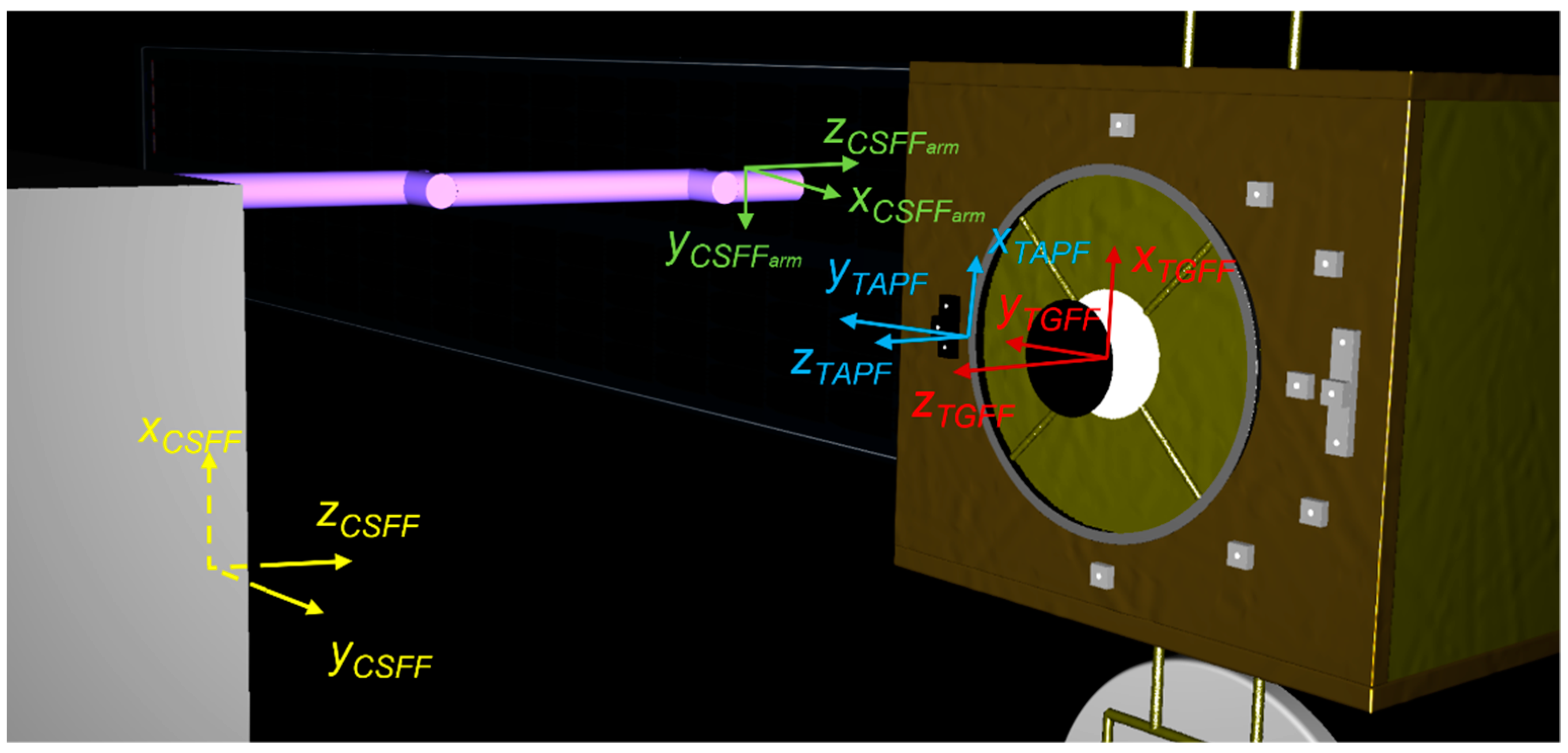
Figure 1.
Target and chaser spacecraft as modelled in PANGU, with representation of the reference frames being employed.
Figure 1.
Target and chaser spacecraft as modelled in PANGU, with representation of the reference frames being employed.
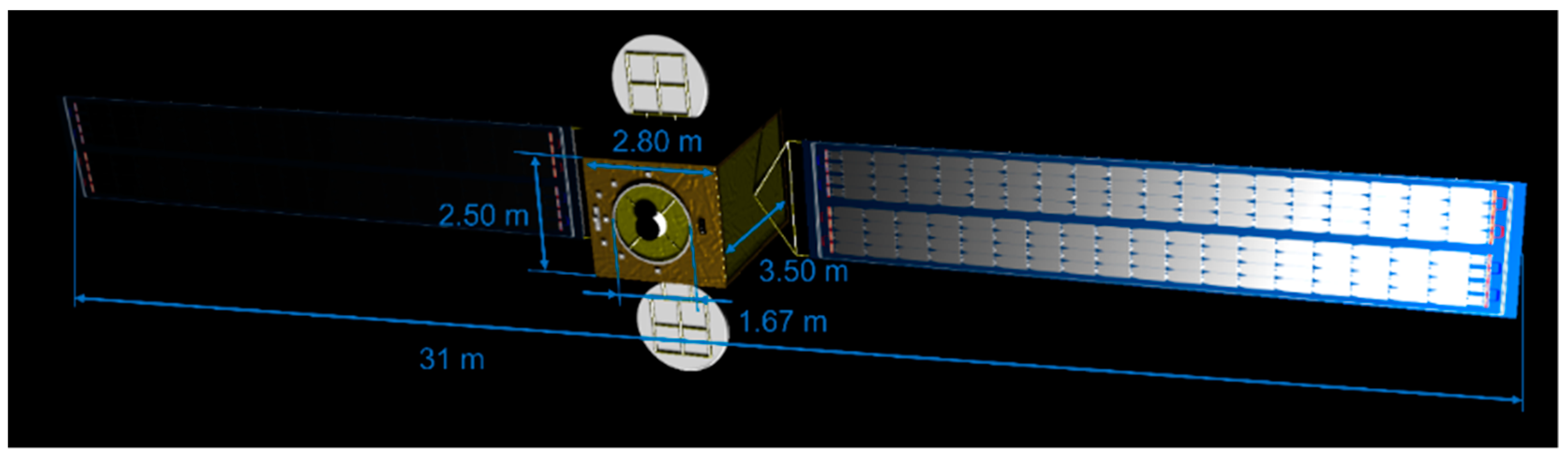
Figure 2.
Target spacecraft model as developed in PANGU, with indication of the main dimensions.
Figure 2.
Target spacecraft model as developed in PANGU, with indication of the main dimensions.
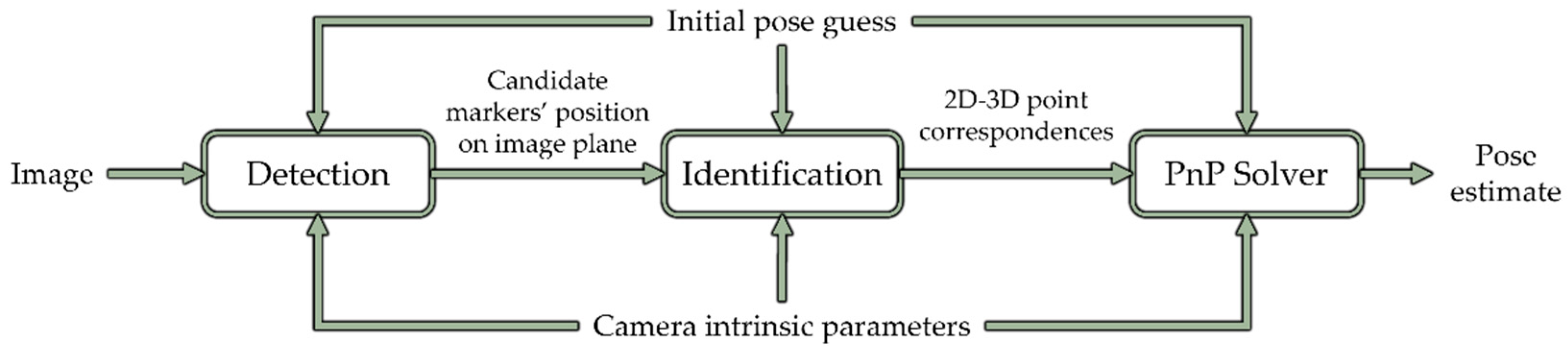
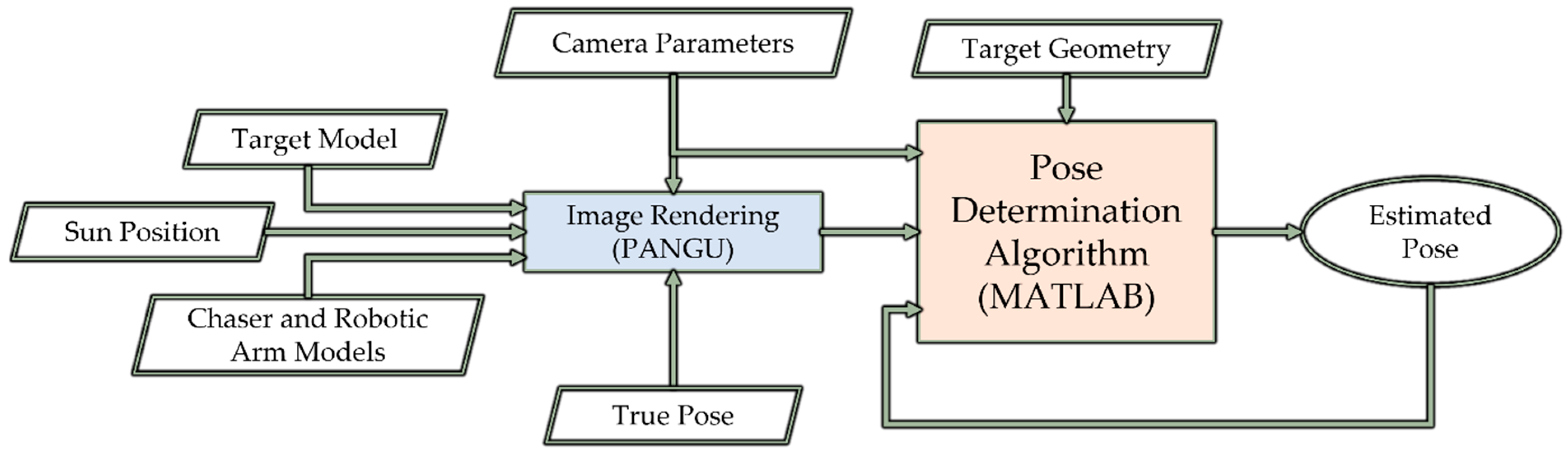
Figure 3.
Flow diagram of the general pose determination architecture employed for pose estimation with the chaser-fixed and eye-in-hand cameras.
Figure 3.
Flow diagram of the general pose determination architecture employed for pose estimation with the chaser-fixed and eye-in-hand cameras.
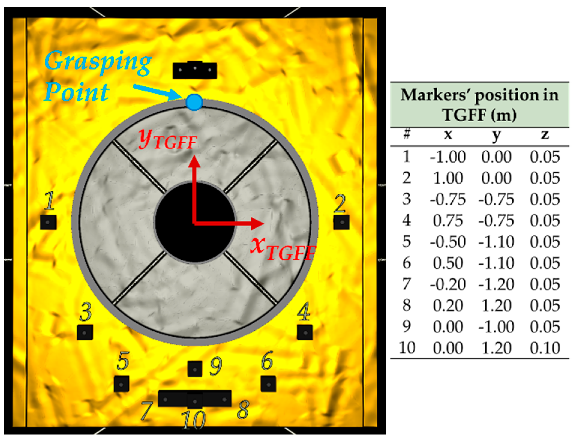
Figure 4.
Pattern of markers employed on the target spacecraft for the CSFF–TGFF pose estimation, with indication of the position vectors in the TGFF.
Figure 4.
Pattern of markers employed on the target spacecraft for the CSFF–TGFF pose estimation, with indication of the position vectors in the TGFF.
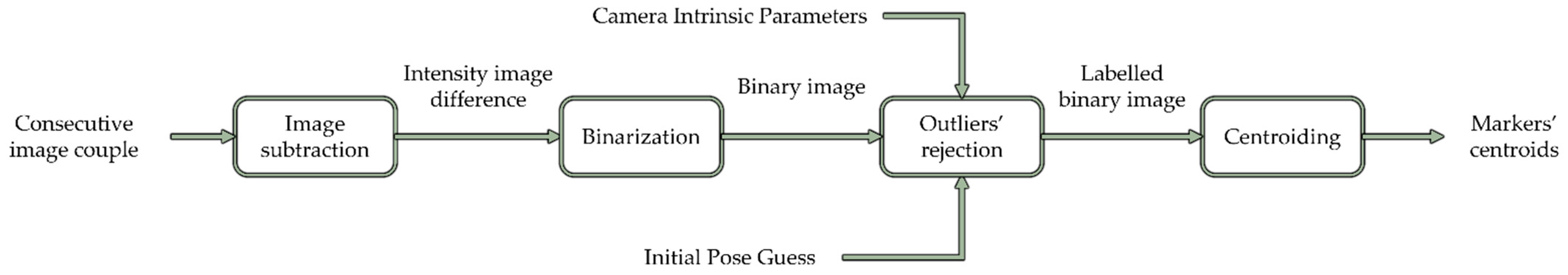
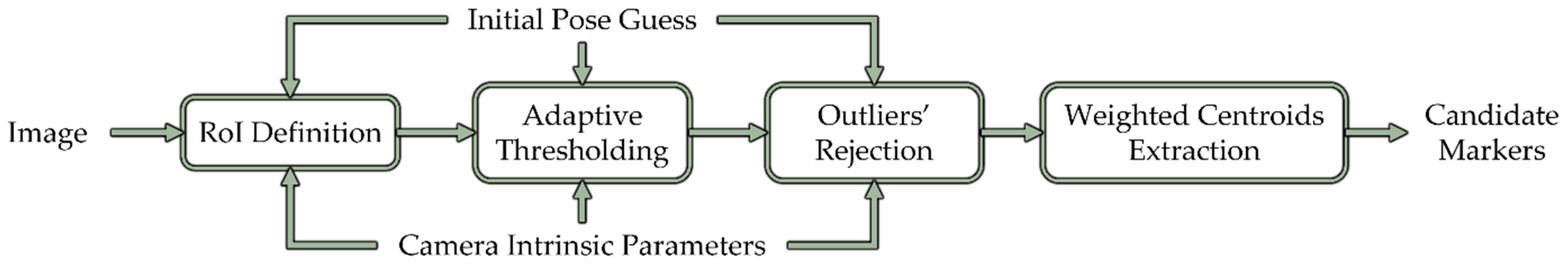
Figure 5.
Flow chart for the detection step proposed for the pose estimation algorithm employing images from the chaser-fixed camera.
Figure 5.
Flow chart for the detection step proposed for the pose estimation algorithm employing images from the chaser-fixed camera.
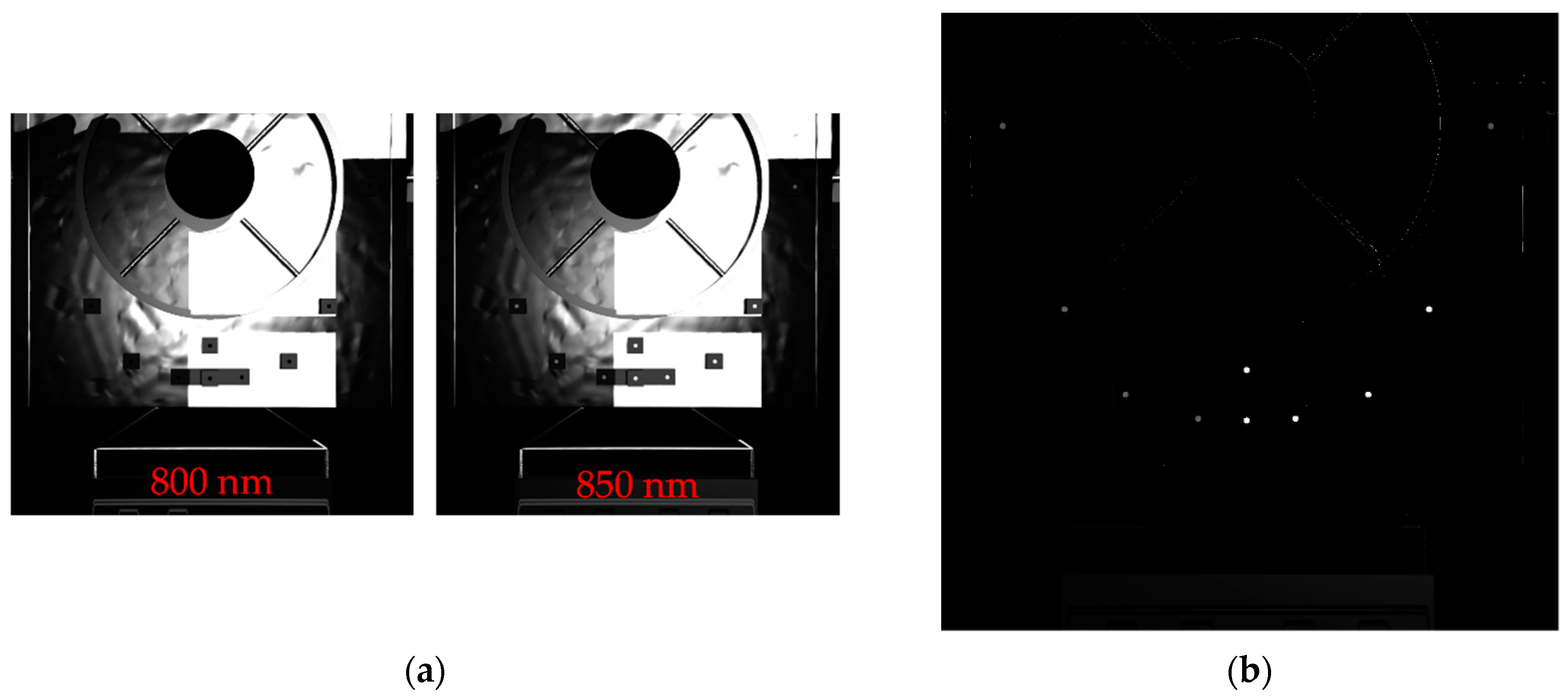
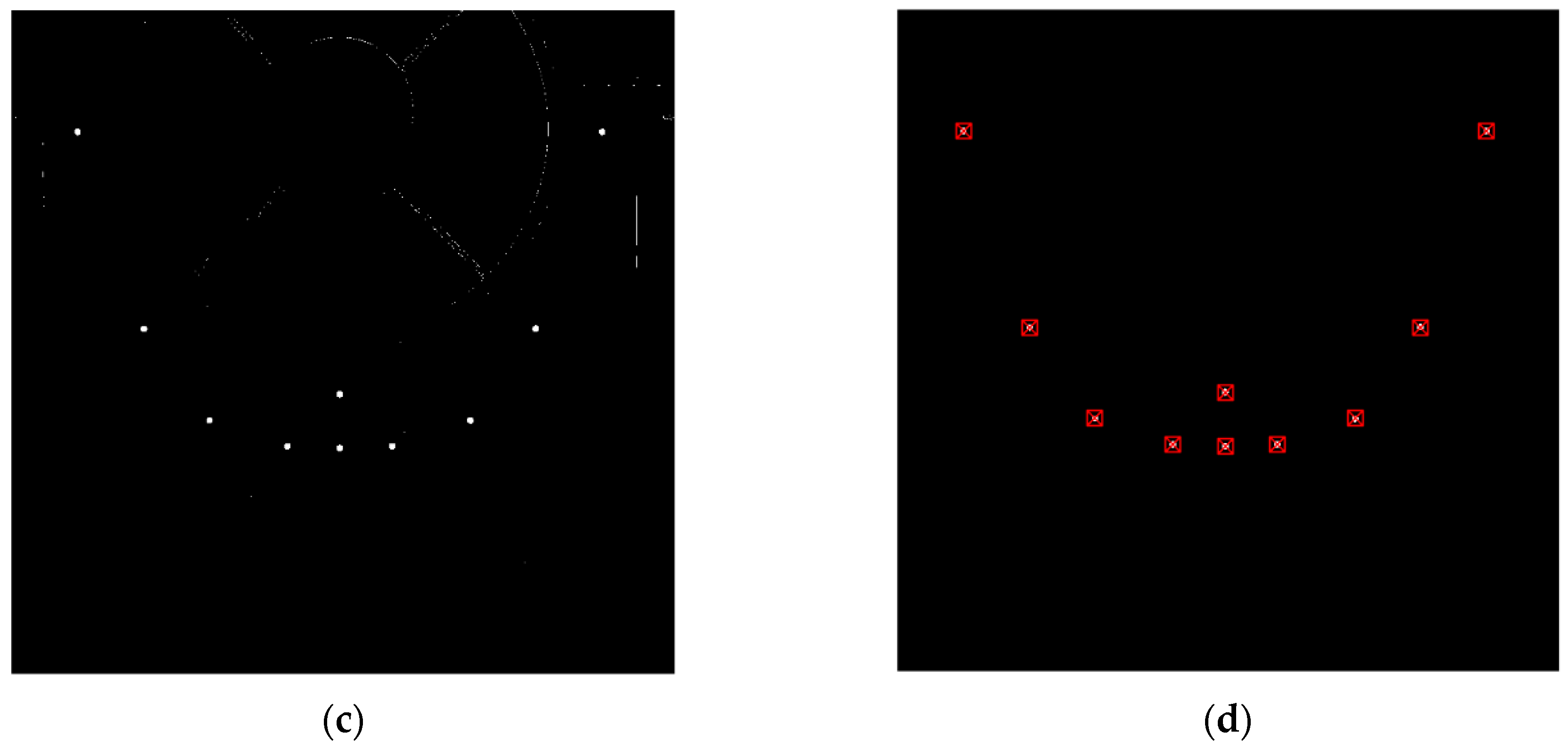
Figure 6.
Image processing pipeline for markers’ detection: (a) two subsequent images illuminating the target asynchronously with the two sources at 800 nm and 850 nm are collected; (b) a difference intensity image is obtained by subtracting the two acquired images; (c) Otsu’s global thresholding is applied to compute the binary mask of the difference image; (d) the weighted centroids of the candidate markers (in red) are finally detected from the binary mask after a sorting process to discard noise and outliers.
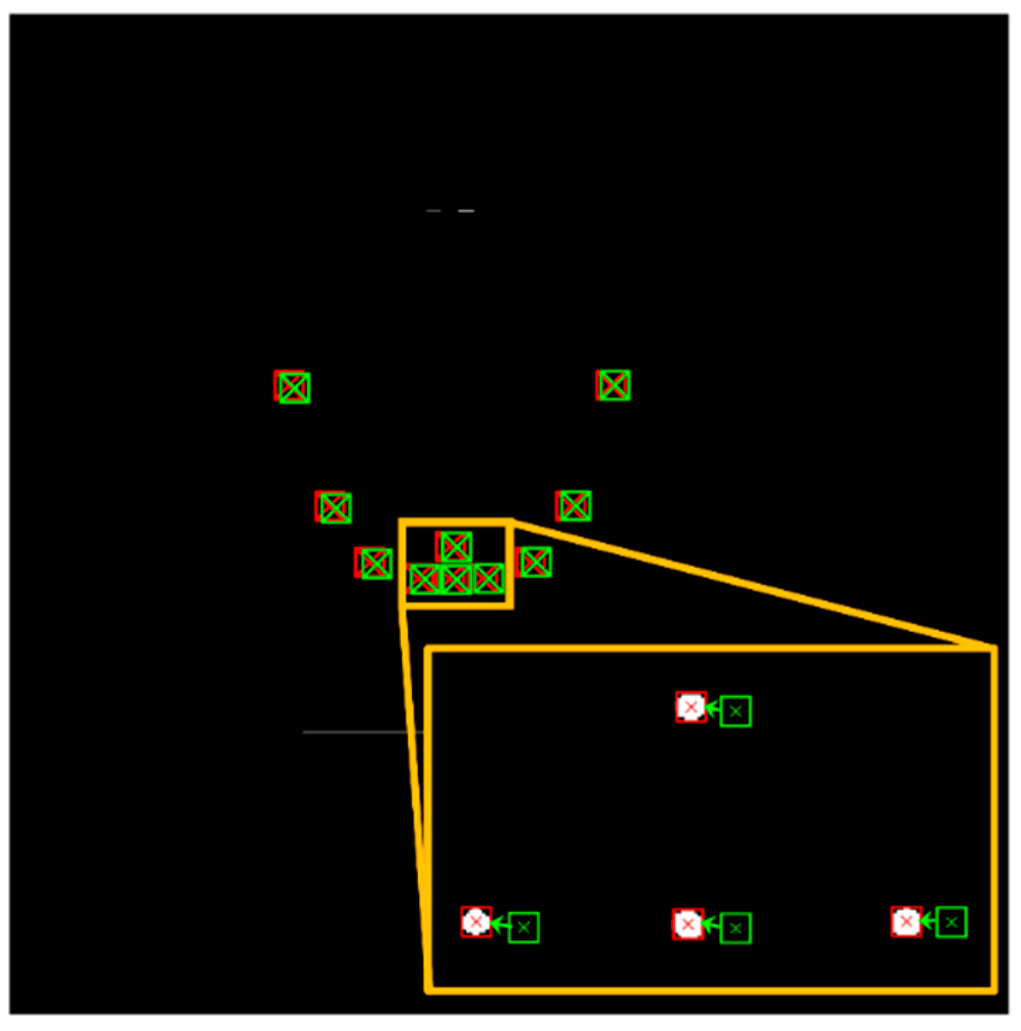
Figure 7.
Graphical depiction of the matching process through Nearest Neighbor. In red: markers’ centroids found through the detection step. In green: markers’ centroids reprojected using the pose initial guess. The arrows show the detected markers to which they are matched. Particular of the matching applied to markers #7 to #10 (in orange box).
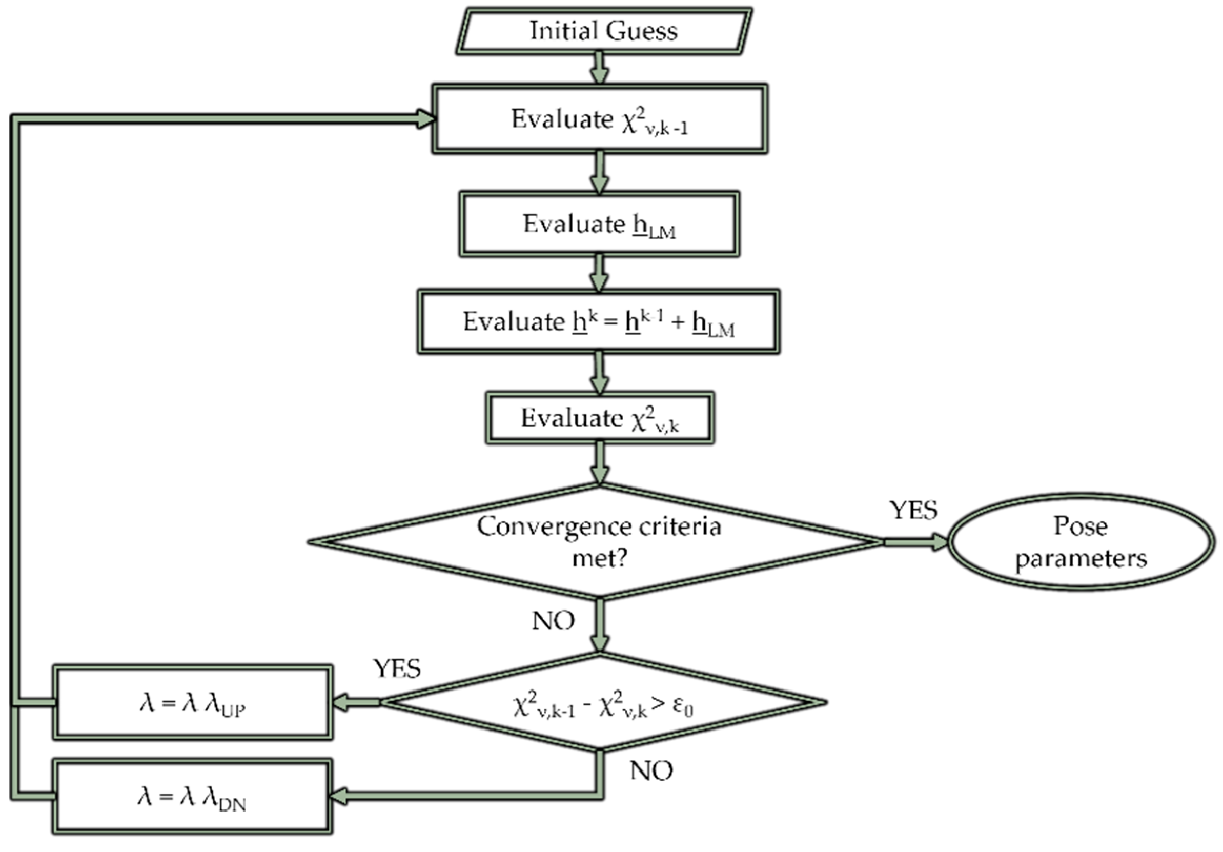
Figure 8.
Flow chart for the proposed implementation of the Levenberg–Marquardt’s iterative method for the least squares non-linear estimation of the pose parameters.
Figure 8.
Flow chart for the proposed implementation of the Levenberg–Marquardt’s iterative method for the least squares non-linear estimation of the pose parameters.
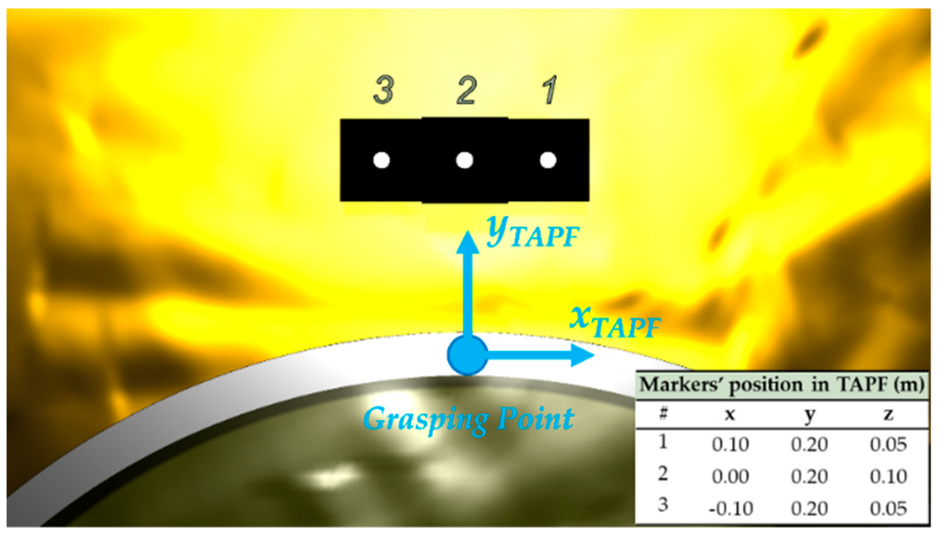
Figure 9.
Pattern of markers employed on the target spacecraft for the CSFFarm-TAPF pose estimation, with indication of the position of their centroids in the TAPF.
Figure 9.
Pattern of markers employed on the target spacecraft for the CSFFarm-TAPF pose estimation, with indication of the position of their centroids in the TAPF.
Figure 10.
Flow chart for the detection step of the algorithm for pose estimation with the eye-in-hand camera.
Figure 10.
Flow chart for the detection step of the algorithm for pose estimation with the eye-in-hand camera.
Figure 11.
Block diagram representation of the simulation environment. The same structure is considered for both the cameras. The trajectory is generated accordingly based on the camera being considered for the simulation.
Figure 11.
Block diagram representation of the simulation environment. The same structure is considered for both the cameras. The trajectory is generated accordingly based on the camera being considered for the simulation.
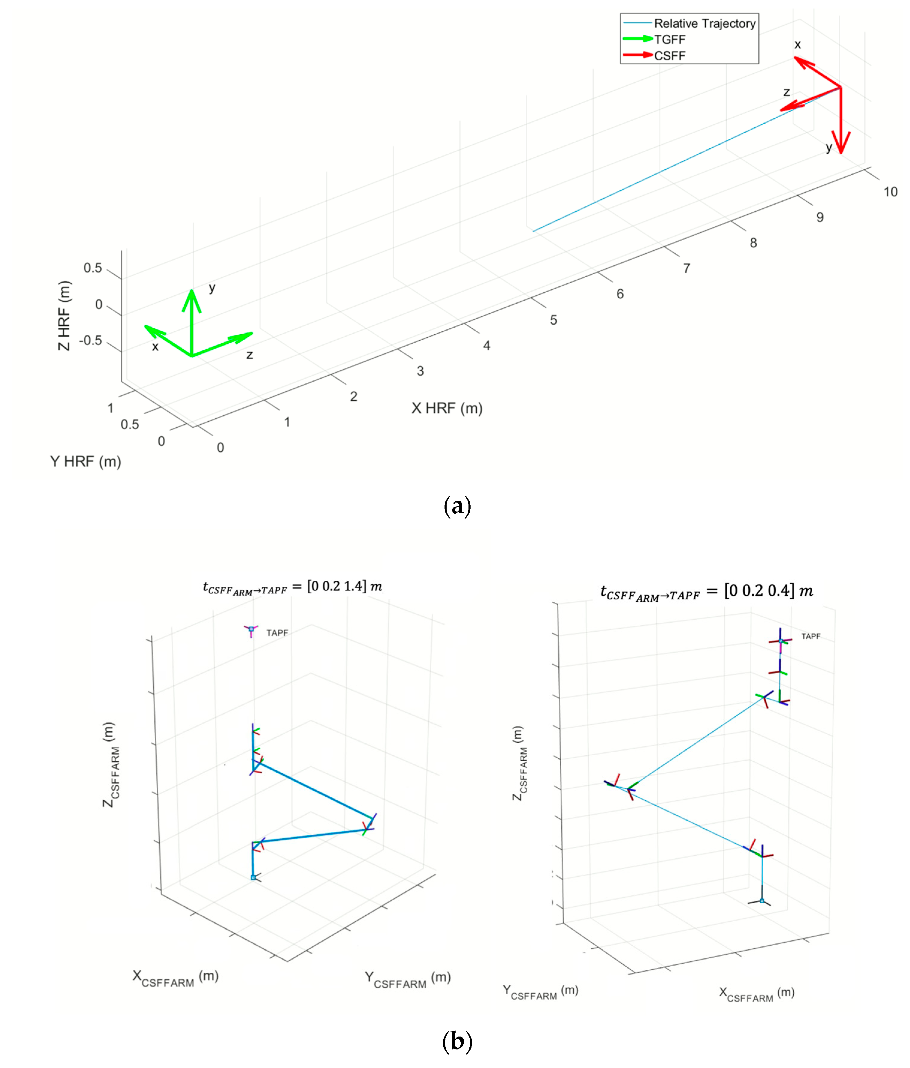
Figure 12.
Relative trajectories employed in the simulations: (a) relative trajectory of the chaser toward the target and the corresponding body-fixed reference frames at scenario start; (b) schematic representation showing the end-effector/grasping point pose corresponding to set-points 2 and 3.
Figure 12.
Relative trajectories employed in the simulations: (a) relative trajectory of the chaser toward the target and the corresponding body-fixed reference frames at scenario start; (b) schematic representation showing the end-effector/grasping point pose corresponding to set-points 2 and 3.
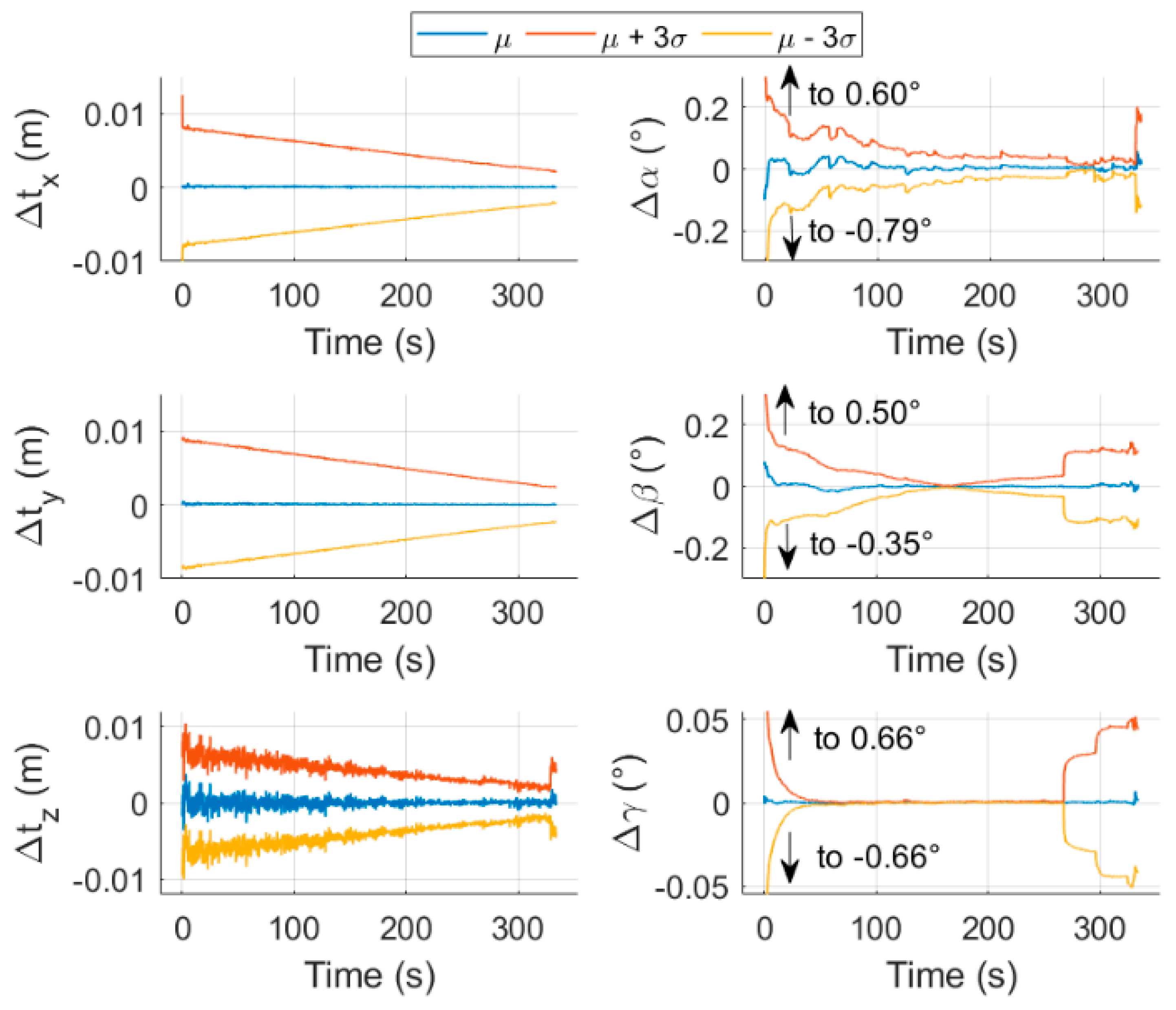
Figure 13.
Temporal evolution of the mean of the errors on the pose parameters, with representation of the 3σ intervals, for test case S1. The plots are focused on intervals about the mean values: the arrows indicate the maximum values reached by the pose initial guess at scenario start.
Figure 13.
Temporal evolution of the mean of the errors on the pose parameters, with representation of the 3σ intervals, for test case S1. The plots are focused on intervals about the mean values: the arrows indicate the maximum values reached by the pose initial guess at scenario start.
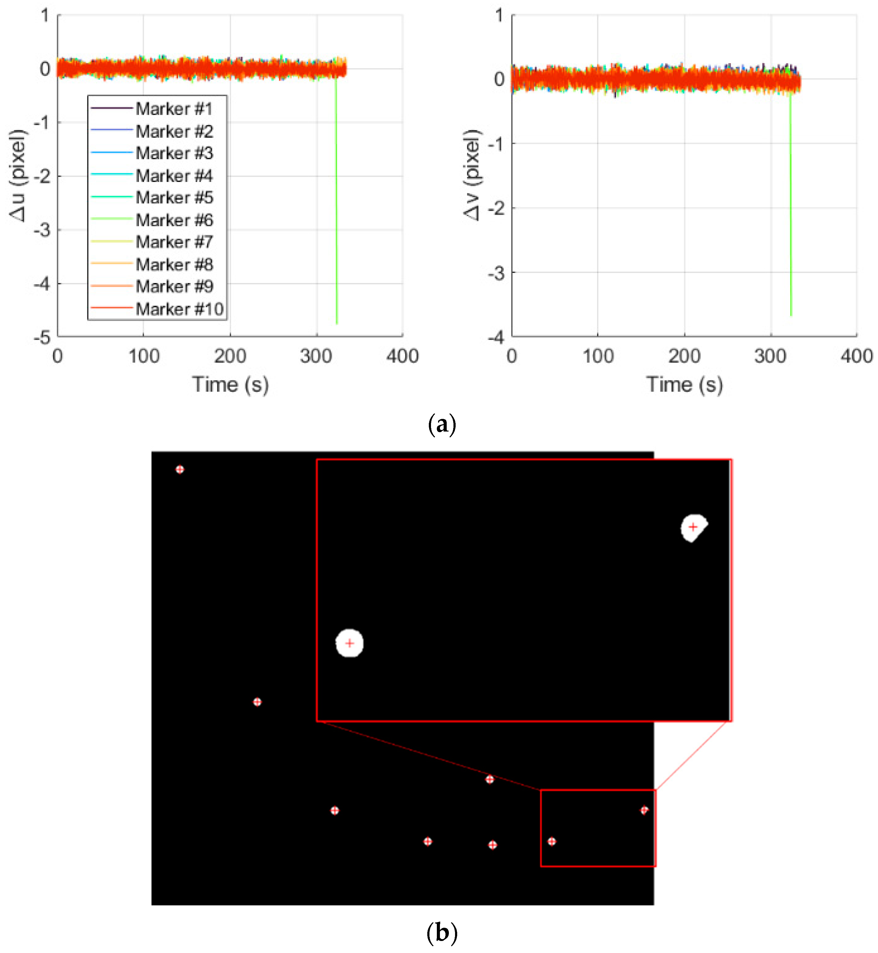
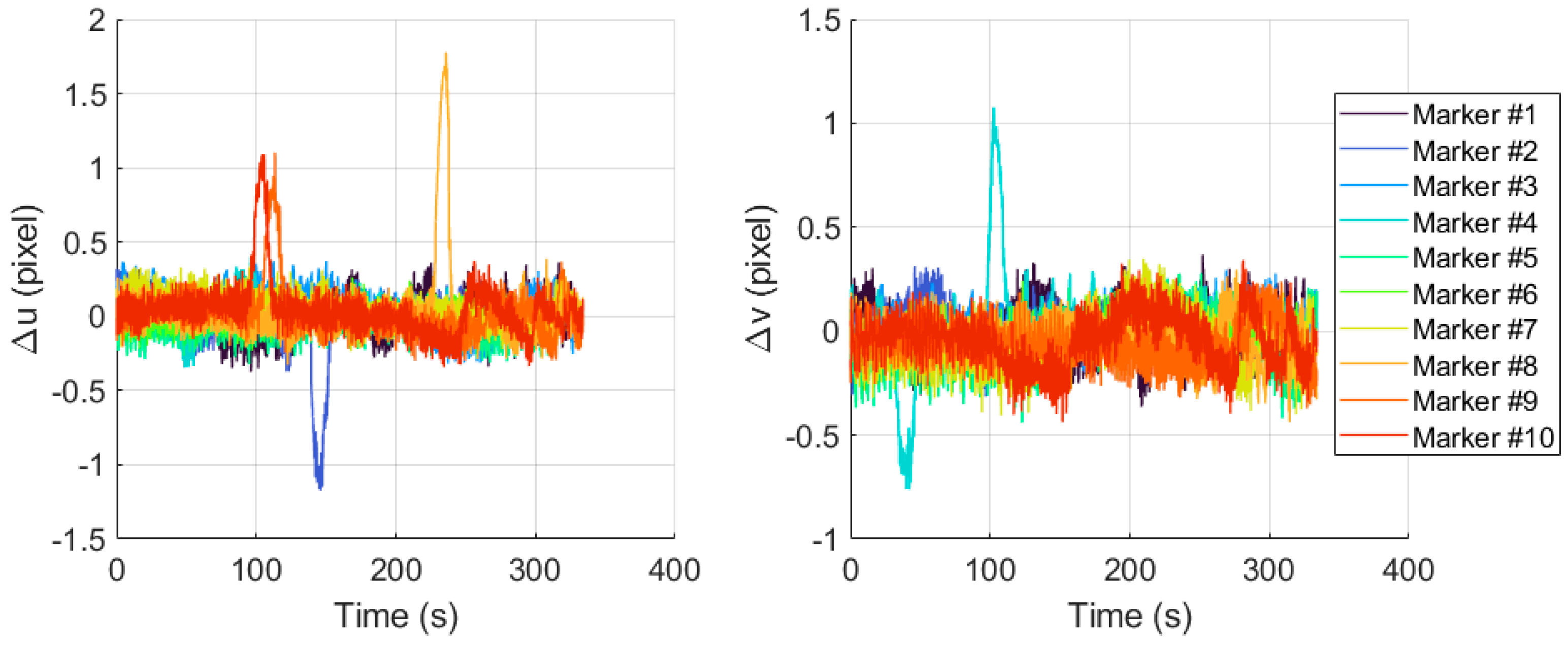
Figure 14.
(a) Temporal evolution of the centroiding errors over a single simulation for test case S3; (b) partial loss of marker #6 at 320 s.
Figure 14.
(a) Temporal evolution of the centroiding errors over a single simulation for test case S3; (b) partial loss of marker #6 at 320 s.
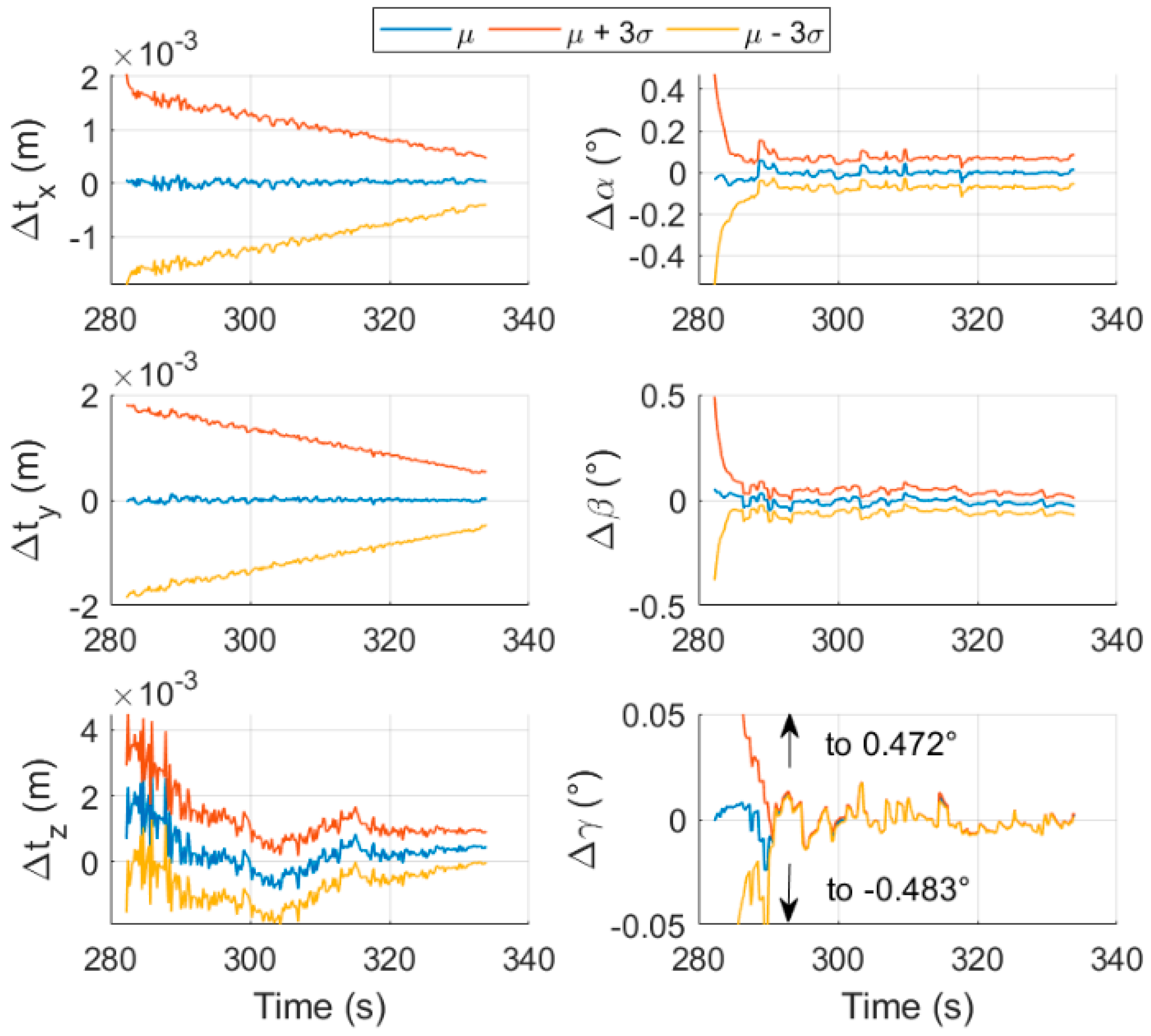
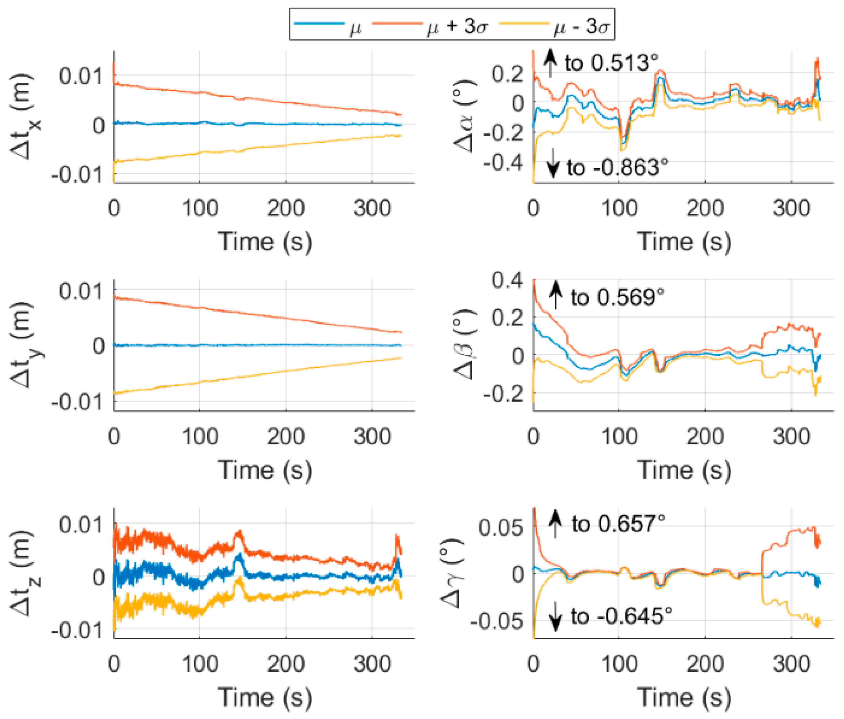
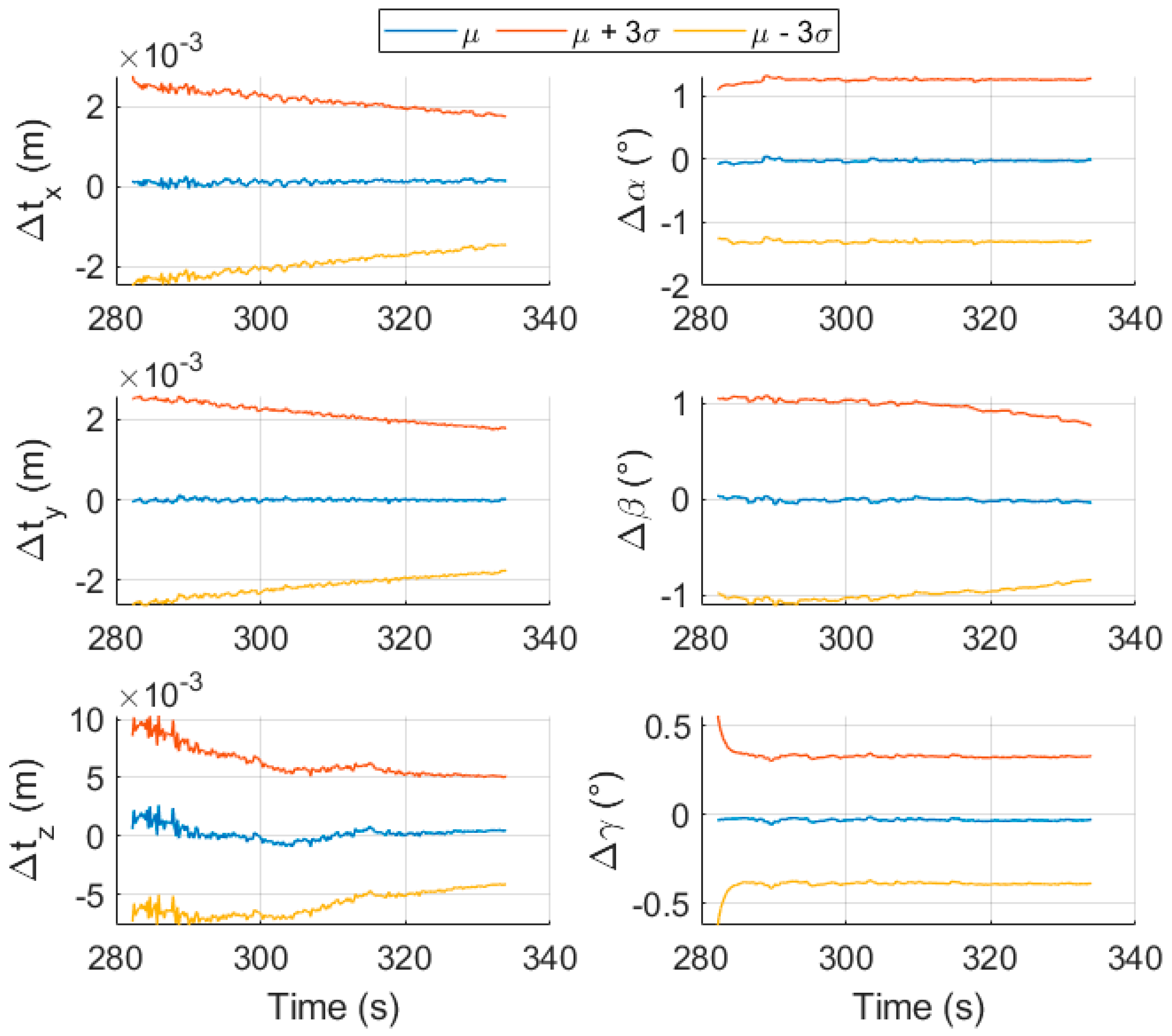
Figure 15.
Temporal evolution of the mean of the errors on the pose parameters, with representation of the 3σ intervals, for test case S7. The plots are focused on intervals about the mean values: the arrows indicate the maximum values reached by the pose initial guess at scenario start.
Figure 15.
Temporal evolution of the mean of the errors on the pose parameters, with representation of the 3σ intervals, for test case S7. The plots are focused on intervals about the mean values: the arrows indicate the maximum values reached by the pose initial guess at scenario start.
Figure 16.
Temporal evolution of the centroiding errors over a single simulation for test cases S7 and I.
Figure 16.
Temporal evolution of the centroiding errors over a single simulation for test cases S7 and I.
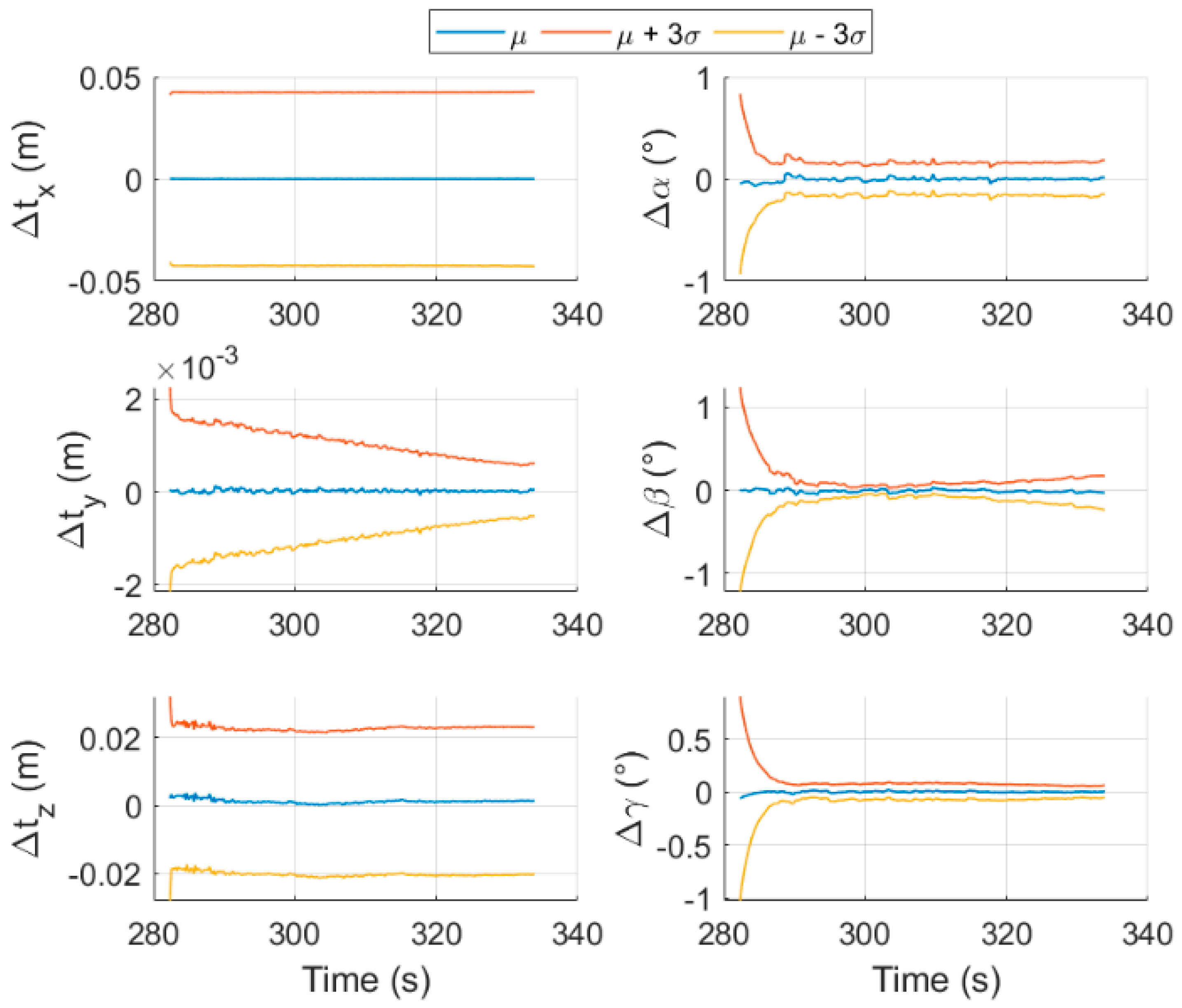
Figure 17.
Temporal evolution of the mean of the errors on the pose parameters, with representation of the 3σ intervals, for test case I. The plots are focused on intervals about the mean values: the arrows indicate the maximum values reached by the pose initial guess at scenario start.
Figure 17.
Temporal evolution of the mean of the errors on the pose parameters, with representation of the 3σ intervals, for test case I. The plots are focused on intervals about the mean values: the arrows indicate the maximum values reached by the pose initial guess at scenario start.
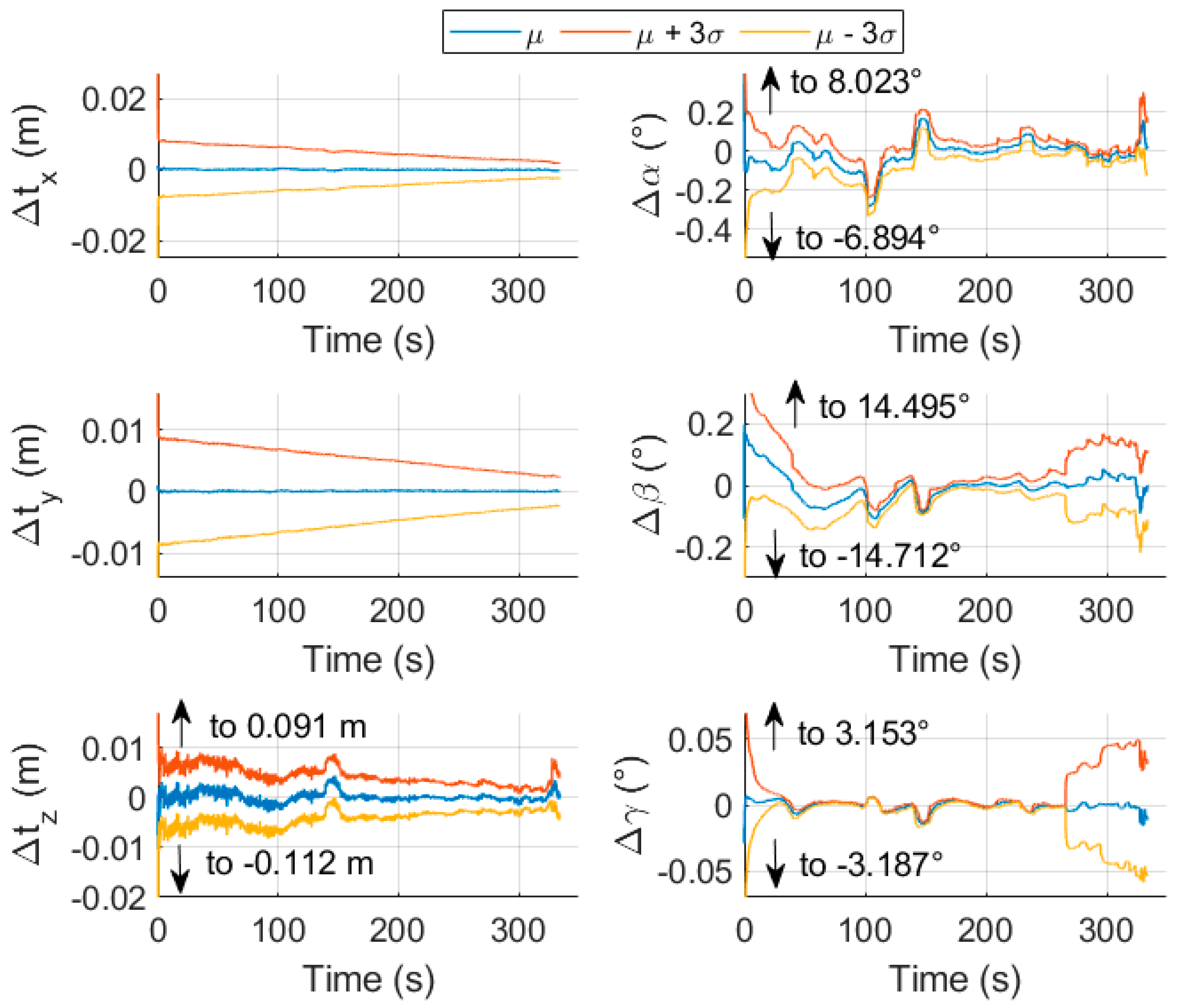
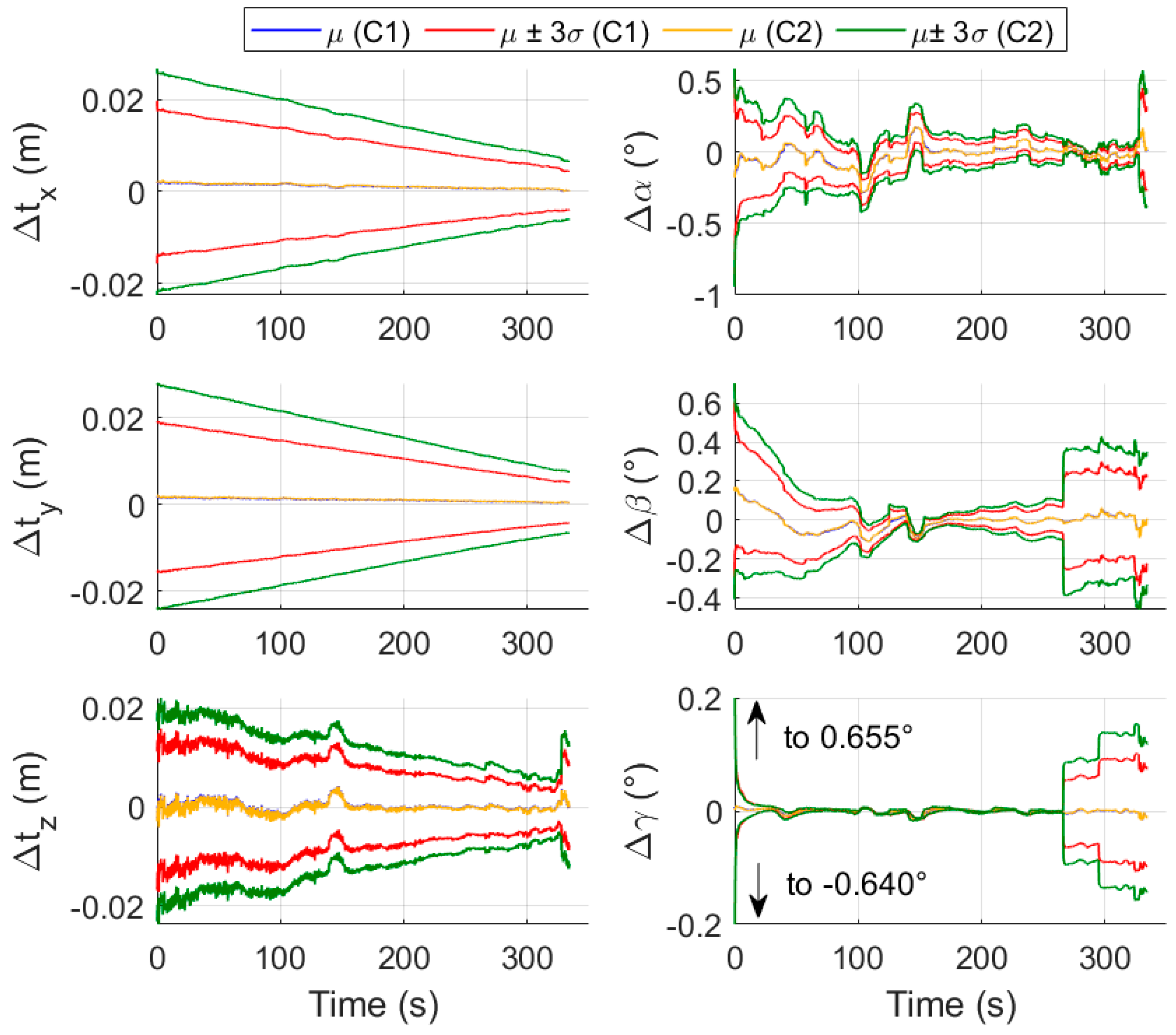
Figure 18.
Temporal evolution of the mean of the errors on the pose parameters, with representation of the 3σ intervals, for tests C1 and C2. The plots are focused on intervals about the mean values: the arrows indicate the maximum values reached by the pose initial guess at scenario start.
Figure 18.
Temporal evolution of the mean of the errors on the pose parameters, with representation of the 3σ intervals, for tests C1 and C2. The plots are focused on intervals about the mean values: the arrows indicate the maximum values reached by the pose initial guess at scenario start.
Figure 19.
Temporal evolution of the mean of the errors on the pose parameters, with representation of the 3σ intervals, for test M1. The plots are focused on intervals about the mean values: the arrows indicate the maximum values reached by the pose initial guess at scenario start.
Figure 19.
Temporal evolution of the mean of the errors on the pose parameters, with representation of the 3σ intervals, for test M1. The plots are focused on intervals about the mean values: the arrows indicate the maximum values reached by the pose initial guess at scenario start.
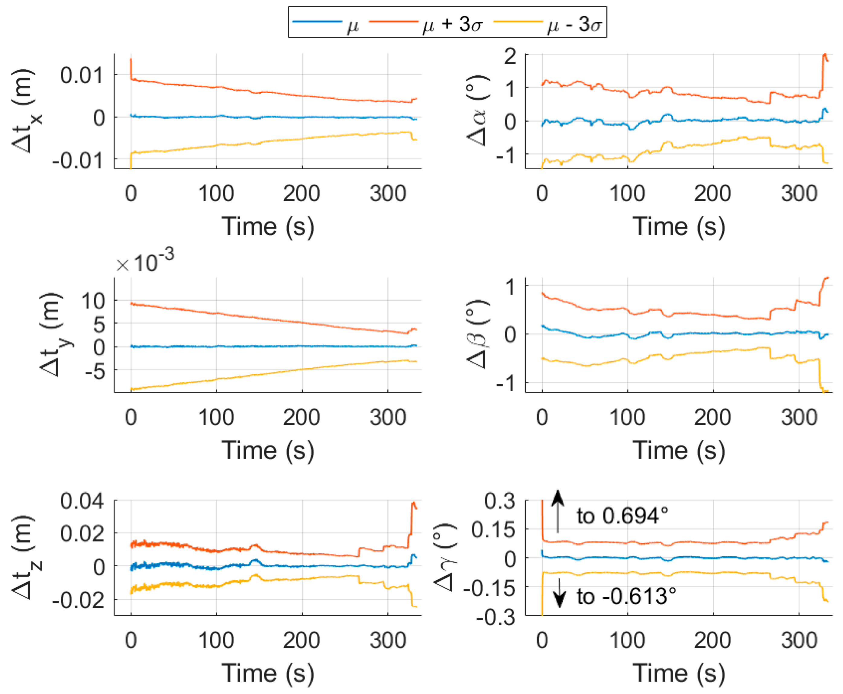
Figure 20.
Temporal evolution of the mean of the errors on the pose parameters, with representation of the 3σ intervals, for test E-SB. The plots are focused on intervals about the mean values: the arrows indicate the maximum values reached by the pose initial guess at scenario start.
Figure 20.
Temporal evolution of the mean of the errors on the pose parameters, with representation of the 3σ intervals, for test E-SB. The plots are focused on intervals about the mean values: the arrows indicate the maximum values reached by the pose initial guess at scenario start.
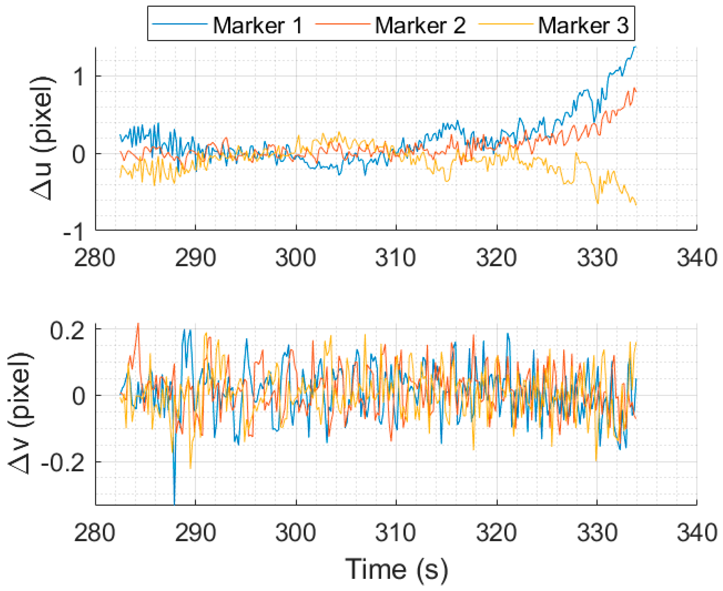
Figure 21.
Temporal evolution of the centroiding errors over a single simulation for test case E-SB.
Figure 21.
Temporal evolution of the centroiding errors over a single simulation for test case E-SB.
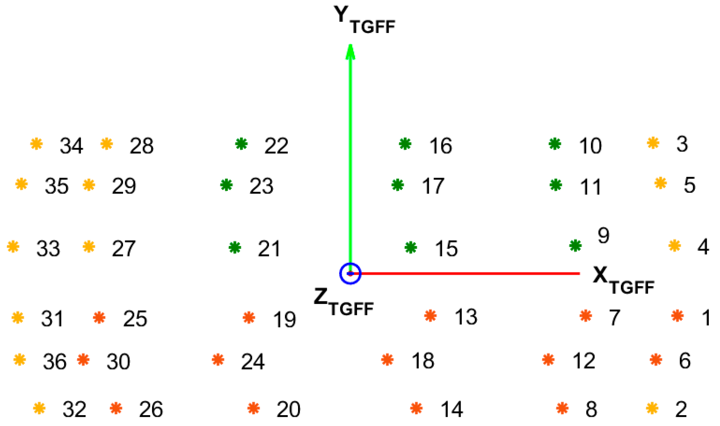
Figure 22.
Qualitative representation of the locations of the Sun in TROF for test cases E-S1 to E-S36 (zTGFF exits the figure’s plane) and their results. In green: cases in which the camera correctly detects all markers at each timestep. In yellow: cases in which part of the markers are lost from a certain timestep. In red: cases in which all the markers are lost from a certain timestep.
Figure 23.
Temporal evolution of the mean of the errors on the pose parameters, with representation of the 3σ intervals, for test case E-I.
Figure 23.
Temporal evolution of the mean of the errors on the pose parameters, with representation of the 3σ intervals, for test case E-I.
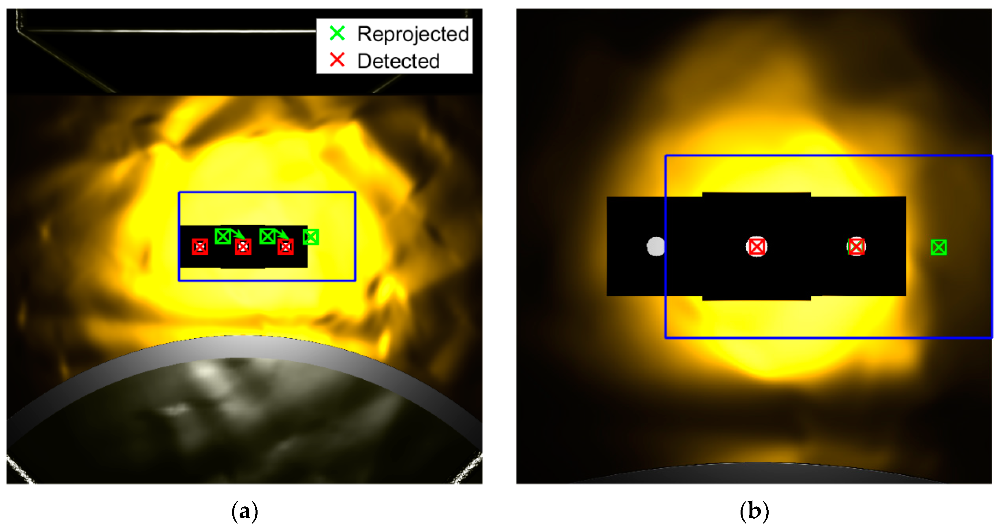
Figure 24.
Consequences of the larger uncertainty on initial conditions, for test case E-I (in blue the RoI): (a) marker mismatch at simulation start caused by the larger uncertainties on the pose initial guess; (b) marker cut out of the RoI, at t = 322.10 s.
Figure 24.
Consequences of the larger uncertainty on initial conditions, for test case E-I (in blue the RoI): (a) marker mismatch at simulation start caused by the larger uncertainties on the pose initial guess; (b) marker cut out of the RoI, at t = 322.10 s.
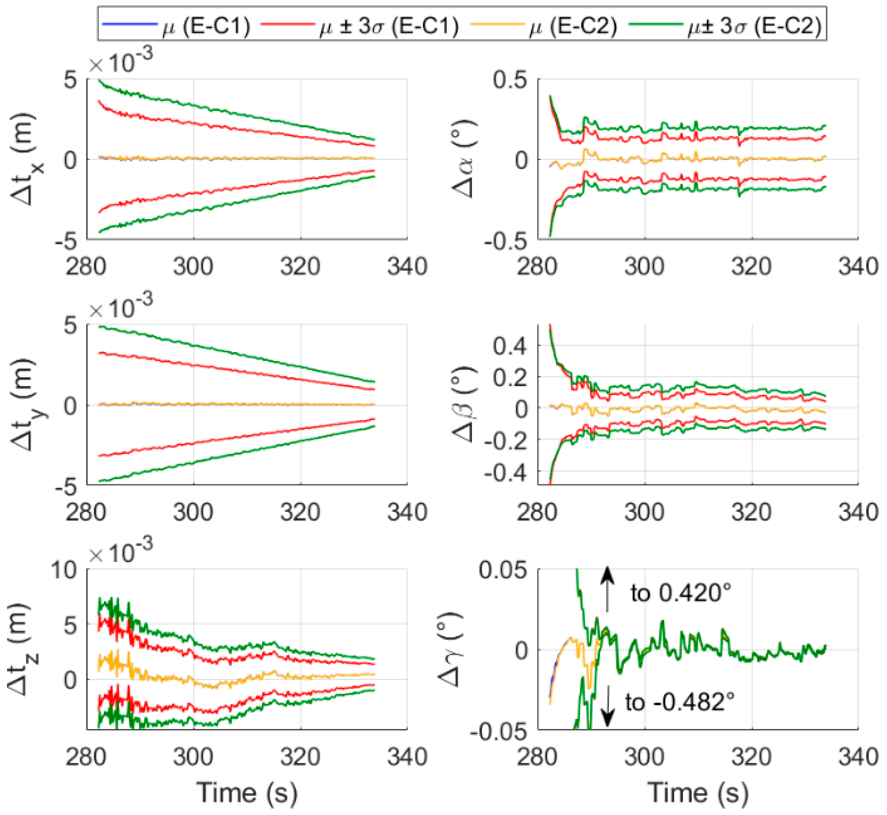
Figure 25.
Temporal evolution of the mean of the errors on the pose parameters, with representation of the 3σ intervals, for tests E-C1 and E-C2.
Figure 25.
Temporal evolution of the mean of the errors on the pose parameters, with representation of the 3σ intervals, for tests E-C1 and E-C2.
Figure 26.
Temporal evolution of the mean of the errors on the pose parameters, with representation of the 3σ intervals, for test E-M1.
Figure 26.
Temporal evolution of the mean of the errors on the pose parameters, with representation of the 3σ intervals, for test E-M1.
Table 1.
Technical specifications of the chaser-fixed camera and its optics, assuming the Teledyne CCD42-40 as detector.
Table 1.
Technical specifications of the chaser-fixed camera and its optics, assuming the Teledyne CCD42-40 as detector.
np (Pixel)
Hor. × Ver. | dp (μm)
Hor. × Ver. | f (cm) | FOV (°)
Hor. × Ver. | IFOV (°)
Hor. × Ver. |
|---|
| 2048 × 2048 | 13.5 × 13.5 | 2.96 | 50 × 50 | 0.0244 × 0.0244 |
Table 2.
Convergence conditions for the proposed implementation of the LM technique for pose determination.
Table 2.
Convergence conditions for the proposed implementation of the LM technique for pose determination.
| Condition | Meaning | Settings |
|---|
| The iterative process is stopped if the normalized pose parameters update term becomes negligible. | ε2 is set to 10−4. Smaller values correspond to variations in the pose estimate to which the algorithm is not sensitive. |
| The iterative process is stopped if the largest component of the gradient in h is smaller than threshold ε1. | ε1 and ε3 are set to very small values, i.e., 10−10 and 10−8, respectively, to ensure stopping close to a minimum of the cost function in the hyper-parameters’ space. |
| The iterative process is stopped if the cost function goes below a threshold. |
Table 3.
Technical specifications of the eye-in-hand camera and its optics, assuming CCD42-40 is used as detector.
Table 3.
Technical specifications of the eye-in-hand camera and its optics, assuming CCD42-40 is used as detector.
Np (Pixel)
Hor. × Ver. | Dp (μm)
Hor. × Ver. | F (cm) | FOV (°)
Hor. × Ver. | IFOV (°)
Hor. × Ver. |
|---|
| 2048 × 2048 | 13.5 × 13.5 | 3.34 | 45 × 45 | 0.0220 × 0.0220 |
Table 4.
Orbital parameters of the target and chaser spacecraft at the beginning of the simulation of the approach.
Table 4.
Orbital parameters of the target and chaser spacecraft at the beginning of the simulation of the approach.
| Spacecraft | Semi-Major Axis (km) | Eccentricity | Inclination (°) | Right Ascension of the Ascending Node | Argument of Perigee (°) | True Anomaly (°) |
|---|
| Target | 42,164 | 1.468 × 10⁻⁷ | 0 | 0 | 0 | 0 |
| Chaser | 42,164.29 | 7.684 × 10⁻⁶ | 6.096 × 10⁻⁵ | 2.565 | 334.093 | 23.34 |
Table 5.
Error level (1σ) in the knowledge of pose initial guesses and camera intrinsic parameters considered in the simulations for both the pose determination with chaser-fixed and eye-in-hand cameras.
Table 5.
Error level (1σ) in the knowledge of pose initial guesses and camera intrinsic parameters considered in the simulations for both the pose determination with chaser-fixed and eye-in-hand cameras.
| Chaser-Fixed Camera |
|---|
| Pose Initial Guess Uncertainty (1σ) | Intrinsic Parameters Uncertainty (1σ) |
|---|
| Tx (m) | Ty (m) | Tz (m) | α (°) | β (°) | γ (°) | fu (px) | fv (px) | cu (px) | cv (px) |
| 0.017 | 0.017 | 0.05 | 1 | 1 | 1 | 1 | 1 | 1 | 1 |
| Eye-in-Hand Camera |
| Pose Initial Guess Uncertainty (1σ) | Intrinsic Parameters Uncertainty (1σ) |
| Tx (m) | Ty (m) | Tz (m) | α (°) | β (°) | γ (°) | fu (px) | fv (px) | cu (px) | cv (px) |
| 0.010 | 0.010 | 0.010 | 0.667 | 0.667 | 0.667 | 1 | 1 | 1 | 1 |
Table 6.
Summary of test cases with variable illumination conditions for the pose estimation with the chaser-fixed camera.
Table 6.
Summary of test cases with variable illumination conditions for the pose estimation with the chaser-fixed camera.
| Test Case | Az (°) | El (°) |
|---|
| S1 | 0 | 90 |
| S2 | 270 | 45 |
| S3 | 270 | 0 |
| S4 | 270 | -60 |
| S5 | 90 | 45 |
| S6 | 90 | 80 |
| S7 | 67 | 75 |
Table 7.
Summary of test cases with variable illumination conditions for the pose estimation with the eye-in-hand camera.
Table 7.
Summary of test cases with variable illumination conditions for the pose estimation with the eye-in-hand camera.
| Test Case | Az (°) | El (°) | Test Case | Az (°) | El (°) | Test Case | Az (°) | El (°) |
|---|
| E-SB | 270 | 0 | E-S13 | 76.50 | −7.01 | E-S25 | 137.25 | −7.33 |
| E-S1 | 16.66 | −7.07 | E-S14 | 77.91 | −22.97 | E-S26 | 137.73 | −22.96 |
| E-S2 | 18.09 | −22.99 | E-S15 | 79.81 | 4.38 | E-S27 | 139.66 | 4.45 |
| E-S3 | 18.31 | 22.38 | E-S16 | 80.14 | 22.15 | E-S28 | 139.98 | 22.18 |
| E-S4 | 19.08 | 4.70 | E-S17 | 81.89 | 14.98 | E-S29 | 141.74 | 15.03 |
| E-S5 | 21.13 | 15.23 | E-S18 | 83.56 | −14.48 | E-S30 | 143.40 | −14.53 |
| E-S6 | 23.72 | −14.42 | E-S19 | 107.33 | −7.36 | E-S31 | 167.18 | −7.30 |
| E-S7 | 46.58 | −7.04 | E-S20 | 107.82 | −22.96 | E-S32 | 168.71 | −23.03 |
| E-S8 | 48.00 | −22.98 | E-S21 | 109.74 | 4.42 | E-S33 | 169.59 | 4.48 |
| E-S9 | 49.01 | 4.74 | E-S22 | 110.06 | 22.16 | E-S34 | 169.90 | 22.19 |
| E-S10 | 50.23 | 22.14 | E-S23 | 111.81 | 15.00 | E-S35 | 171.66 | 15.05 |
| E-S11 | 51.97 | 14.95 | E-S24 | 113.48 | −14.50 | E-S36 | 173.32 | −14.56 |
| E-S12 | 53.64 | −14.45 | | | | | | |
Table 8.
Summary of test cases with variable accuracy on the initialization of the pose solution for both the pose estimation with the chaser-fixed and the eye-in-hand cameras.
Table 8.
Summary of test cases with variable accuracy on the initialization of the pose solution for both the pose estimation with the chaser-fixed and the eye-in-hand cameras.
| Pose Estimation with Chaser-Fixed Camera | Pose Estimation with Eye-in-Hand Camera |
|---|
| Test Case | Description of Test Conditions | Test Case | Description of Test Conditions |
|---|
| I | Noise on the initial pose guess has twice the standard deviations indicated in Table 5 | E-I | Noise on the initial pose guess has twice the standard deviations indicated in Table 5 |
Table 9.
Summary of test cases with variable accuracy on the knowledge of the camera intrinsic parameters for both the pose estimation with the chaser-fixed and the eye-in-hand cameras.
Table 9.
Summary of test cases with variable accuracy on the knowledge of the camera intrinsic parameters for both the pose estimation with the chaser-fixed and the eye-in-hand cameras.
| Pose Estimation with Chaser-Fixed Camera | Pose Estimation with Eye-in-Hand Camera |
|---|
| Test Case | Description of Test Conditions | Test Case | Description of Test Conditions |
|---|
| C1 | Noise on the camera intrinsic parameters has twice the standard deviations indicated in Table 5. | E-C1 | Noise on the camera intrinsic parameters has twice the standard deviations indicated in Table 5. |
| C2 | Noise on the camera intrinsic parameters has thrice the standard deviations indicated in Table 5. | E-C2 | Noise on the camera intrinsic parameters has thrice the standard deviations indicated in Table 5. |
Table 10.
Summary of test cases with errors in the positioning of the markers on the target for both the pose estimation with the chaser-fixed and the eye-in-hand cameras.
Table 10.
Summary of test cases with errors in the positioning of the markers on the target for both the pose estimation with the chaser-fixed and the eye-in-hand cameras.
| Pose Estimation with Chaser-Fixed Camera | Pose Estimation with Eye-in-Hand Camera |
|---|
| Test Case | Description of Test Conditions | Test Case | Description of Test Conditions |
|---|
| M1 | Error in markers’ positioning with standard deviation of 1 mm. | E-M1 | Error in markers’ positioning with standard deviation of 0.3 mm. |
Table 11.
Summary of the setting parameters employed for the pose estimation algorithms with both the chaser-fixed and eye-in-hand cameras.
Table 11.
Summary of the setting parameters employed for the pose estimation algorithms with both the chaser-fixed and eye-in-hand cameras.
| Setting of Parameters—Pose Estimation with Chaser-Fixed Camera |
|---|
Detection and
Identification | Pose Estimation |
|---|
| τbin | 0.2 | sbord | 1.2 | ε0 | 10−9 | nmax,it | 200 |
| τcirc | 0.5 | sid | 2 | ε1 | 10−10 | λ0 | 10−8 |
| sao | 0.6 | | | ε2 | 10−4 | λUP | 11 |
| | | | | ε3 | 10−8 | λDN | 9 |
| Setting of Parameters—Pose Estimation with Eye-in-Hand Camera |
Detection and
Identification | Pose Estimation |
| τcirc | 0.5 | [scu, scy] | [2, 2] | ε0 | 10−9 | nmax,it | 200 |
| sao | 0.25 | τs | 0.3 | ε1 | 10−10 | λ0 | 10−8 |
| [sx, sy] | [0.5, 0.5] | sid | 2 | ε2 | 10−4 | λUP | 11 |
| | | | | ε3 | 10−8 | λDN | 9 |
Table 12.
Mean and standard deviation of the pose estimation errors for test cases S1 to S7.
Table 12.
Mean and standard deviation of the pose estimation errors for test cases S1 to S7.
| Test Case | Statistic | Δtx (cm) | Δty (cm) | Δtz (cm) | Δα (°) | Δβ (°) | Δγ (°) |
|---|
| S1 | μN | 0.009 | 0.008 | 0.0004 | 0.007 | 0.0002 | 0.0003 |
| σN | 0.007 | 0.007 | 0.056 | 0.014 | 0.009 | 0.0005 |
| S2 | μN | 0.009 | 0.008 | −0.00004 | 0.008 | 0.0007 | 0.0004 |
| σN | 0.007 | 0.007 | 0.056 | 0.013 | 0.009 | 0.0006 |
| S3 | μN | 0.005 | 0.009 | 0.030 | 0.018 | −0.014 | −0.0003 |
| σN | 0.010 | 0.011 | 0.195 | 0.085 | 0.093 | 0.002 |
| S4 | μN | 0.008 | 0.008 | 0.034 | 0.018 | −0.015 | −0.0001 |
| σN | 0.010 | 0.011 | 0.193 | 0.084 | 0.092 | 0.002 |
| S5 | μN | 0.009 | 0.007 | 0.001 | 0.007 | −0.002 | −0.0001 |
| σN | 0.007 | 0.007 | 0.056 | 0.013 | 0.009 | 0.0005 |
| S6 | μN | 0.009 | 0.008 | −0.0005 | 0.010 | −0.0003 | 0.0001 |
| σN | 0.007 | 0.007 | 0.0006 | 0.014 | 0.009 | 0.0006 |
| S7 | μN | 0.009 | 0.002 | 0.012 | −0.017 | −0.006 | −0.0006 |
| σN | 0.014 | 0.008 | 0.105 | 0.071 | 0.048 | 0.004 |
Table 13.
Mean and standard deviation of the centroiding error over all markers, computed over a single simulation for each test case, for test cases S1 to S7.
Table 13.
Mean and standard deviation of the centroiding error over all markers, computed over a single simulation for each test case, for test cases S1 to S7.
| Statistic | Parameter | Test Cases |
|---|
| S1 | S2 | S3 | S4 | S5 | S6 | S7 |
|---|
| Δu (pixel) | Mean | 0.002 | −0.001 | −0.011 | 0.002 | 0.008 | 0.008 | 0.015 |
| Std | 0.076 | 0.075 | 0.094 | 0.093 | 0.075 | 0.074 | 0.159 |
| Δv (pixel) | Mean | −0.003 | −0.0002 | −0.005 | −0.013 | −0.006 | −0.002 | −0.024 |
| Std | 0.078 | 0.077 | 0.091 | 0.091 | 0.077 | 0.077 | 0.127 |
Table 14.
Mean and standard deviation of the pose estimation errors for a higher uncertainty in the knowledge of the initial condition, for test case I.
Table 14.
Mean and standard deviation of the pose estimation errors for a higher uncertainty in the knowledge of the initial condition, for test case I.
| Test Case | Statistic | Δtx (cm) | Δty (cm) | Δtz (cm) | Δα (°) | Δβ (°) | Δγ (°) |
|---|
| I | μN | 0.010 | 0.003 | 0.011 | −0.016 | −0.006 | −0.0007 |
| σN | 0.015 | 0.009 | 0.108 | 0.072 | 0.048 | 0.004 |
Table 15.
Mean and standard deviation of the pose estimation errors for different levels of uncertainty in the knowledge of the intrinsic parameters of the camera for test cases C1 and C2.
Table 15.
Mean and standard deviation of the pose estimation errors for different levels of uncertainty in the knowledge of the intrinsic parameters of the camera for test cases C1 and C2.
| Test Case | Statistic | Δtx (cm) | Δty (cm) | Δtz (cm) | Δα (°) | Δβ (°) | Δγ (°) |
|---|
| C1 | μN | 0.018 | 0.010 | 0.003 | −0.017 | −0.005 | −0.0004 |
| σN | 0.016 | 0.008 | 0.104 | 0.072 | 0.047 | 0.004 |
| C2 | μN | 0.026 | 0.018 | −0.005 | −0.016 | −0.005 | −0.0003 |
| σN | 0.018 | 0.009 | 0.103 | 0.072 | 0.047 | 0.004 |
Table 16.
Mean and standard deviation of the pose estimation errors in presence of uncertainties in the positioning of the markers on the target for test case M1.
Table 16.
Mean and standard deviation of the pose estimation errors in presence of uncertainties in the positioning of the markers on the target for test case M1.
| Test Case | Statistic | Δtx (cm) | Δty (cm) | Δtz (cm) | Δα (°) | Δβ (°) | Δγ (°) |
|---|
| M1 | μN | −0.008 | 0.003 | 0.017 | −0.0003 | 0.0003 | −0.001 |
| σN | 0.015 | 0.009 | 0.129 | 0.087 | 0.046 | 0.005 |
Table 17.
Mean and standard deviation of the pose estimation errors for test case E-SB.
Table 17.
Mean and standard deviation of the pose estimation errors for test case E-SB.
| Test Case | Statistic | Δtx (cm) | Δty (cm) | Δtz (cm) | Δα (°) | Δβ (°) | Δγ (°) |
|---|
| E-SB | μN | 0.002 | 0.0003 | 0.031 | −0.004 | −0.007 | −0.0004 |
| σN | 0.005 | 0.003 | 0.061 | 0.019 | 0.019 | 0.006 |
Table 18.
Mean and standard deviation of the pose estimation errors for different levels of uncertainty in the knowledge of the initial condition, for test case E-I.
Table 18.
Mean and standard deviation of the pose estimation errors for different levels of uncertainty in the knowledge of the initial condition, for test case E-I.
| Test Case | Statistic | Δtx (cm) | Δty (cm) | Δtz (cm) | Δα (°) | Δβ (°) | Δγ (°) |
|---|
| E-I | μN | 0.002 | 0.002 | 0.130 | −0.003 | −0.008 | 0.001 |
| σN | 0.006 | 0.003 | 0.062 | 0.019 | 0.016 | 0.010 |
Table 19.
Mean and standard deviation of the pose estimation errors for different levels of uncertainty in the knowledge of the camera intrinsic parameters, for test cases E-C1 and E-C2.
Table 19.
Mean and standard deviation of the pose estimation errors for different levels of uncertainty in the knowledge of the camera intrinsic parameters, for test cases E-C1 and E-C2.
| Test Case | Statistic | Δtx (cm) | Δty (cm) | Δtz (cm) | Δα (°) | Δβ (°) | Δγ (°) |
|---|
| E-C1 | μN | 0.004 | 0.003 | 0.026 | −0.003 | −0.007 | −0.001 |
| σN | 0.005 | 0.003 | 0.060 | 0.019 | 0.017 | 0.007 |
| E-C2 | μN | 0.005 | 0.004 | 0.025 | −0.002 | −0.007 | −0.001 |
| σN | 0.005 | 0.004 | 0.060 | 0.019 | 0.017 | 0.007 |
Table 20.
Mean and standard deviation of the pose estimation errors in presence of uncertainties in the positioning of the markers on the target, for test case E-M1.
Table 20.
Mean and standard deviation of the pose estimation errors in presence of uncertainties in the positioning of the markers on the target, for test case E-M1.
| Test Case | Statistic | Δtx (cm) | Δty (cm) | Δtz (cm) | Δα (°) | Δβ (°) | Δγ (°) |
|---|
| E-M1 | μN | 0.012 | −0.0003 | 0.026 | −0.027 | −0.005 | −0.03 |
| σN | 0.005 | 0.003 | 0.059 | 0.019 | 0.018 | 0.006 |


