Uncertainty Assessment of Differential Absorption Lidar Measurements of Industrial Emissions Concentrations

Abstract

Differential absorption lidar (DIAL) has been shown to be a very effective technique for the location and quantification of emissions of pollutants and greenhouse gases at industrial facilities. Several field trials have demonstrated the DIAL system performances and contributed to the development of the DIAL methodology, which is the basis of the protocols described in the European Standard EN 17628. While numerous papers have focused on different aspects of DIAL uncertainties, a rigorous propagation of the uncertainties in the DIAL equation has not been found. In this study, all the uncertainty sources contributing to a DIAL concentration measurement are assessed and the impact they have on the calculation of the mass emission rate. We derive the equations for both a DIAL system path-concentration integral and concentration uncertainties. The results from a methane measurement are presented, showing that for a signal to noise ratio on the backscattered lidar signals of 500, the path-concentration integral standard uncertainty is 2.3 ppb km and the concentration standard uncertainty is 92 ppb over a sampling spacing of 45 m. An equation is also presented enabling calculation of the contribution of the concentration uncertainty to the mass emission rate uncertainty.

1. Introduction

The European Union, as part of its Industrial Emissions Directive 2010/75/EU, has published the Best Available Techniques (BAT) reference document for the refining of mineral oil and gas [1]. The BAT conclusion includes differential absorption lidar (DIAL) as a technique to monitor diffuse volatile organic compound (VOC) emissions from an industrial site. In response to this, the European Committee for Standardisation (CEN) produced a new standard, EN 17628 [2], for the use of systems such as DIAL to monitor the fugitive emissions of VOCs.

DIAL is a remote sensing laser-based technique capable of making spatially resolved measurements of concentrations of a target gas along the path of a laser beam transmitted into the atmosphere [3]. It combines the use of light detection and ranging (lidar) to measure back-scattered light from the atmosphere and the targeted species at two known, pre-selected, wavelengths of light. One of these (λ_on) is strongly absorbed by the species of interest while the second pulse (λ_off) is at a wavelength that has a much weaker absorption. The difference in the absorption of the two wavelengths allows the concentration of the gas to be calculated along the optical path. The ability to scan the optical measurement beam through a vertical plane in the atmosphere enables the gas concentrations to be mapped within the atmosphere and the emission rates to be determined when the concentration data are combined with wind data.

The mobile DIAL systems developed at the National Physical Laboratory (NPL) for the remote measurements of pollutants and greenhouse gases have been used worldwide for over 30 years at different industrial facilities such as refineries, liquid natural gas terminals, tank farms, biogas, wastewaters, and landfills utilising both the ultraviolet (UV) and infrared (IR) regions for different species such as volatile organic compound (VOCs), methane, ethane, SO₂, NO_x, HCl, and benzene [4,5,6,7].

In a DIAL system, the two wavelengths are selected to have a small wavelength separation to minimise differences in atmospheric scattering and interference compounds and therefore minimise the effect on the concentration measurements from the parameters describing atmospheric variability in the lidar equation [3]. These terms are assumed to be the same for both on and off wavelengths and are then cancelled by taking the ratio of the on and off returned signals in the DIAL Equation (1). The potential sources of uncertainties from this assumption, such as the backscatter and extension coefficients in the lidar equation, have been extensively discussed by previous authors [8,9,10,11,12,13,14]. These works were focused on DIAL nadir or zenith measurements, hence looking at backscatter and extension coefficients variations over several kilometres into the troposphere and lower stratosphere rather than measurements at industrial facilities over just a few hundred meters within the boundary layer. In such applications plumes of gases, vapour and heat sources at industrial facilities can limit the sensitivity of the DIAL as a consequence of differences in the backscatter coefficients between the on and off beams. This can be caused by a number of factors such as imperfect beam overlap, movement of the atmosphere, inhomogeneities between the on and off pulses, and differences between the detection system collection efficiencies due to the asymmetries in the transmitted on and off beams as described in detail in the work of Walmsley and O’Connor [15]. Most previous DIAL uncertainty papers addressed the variance of the return on and off signals as proportional to the signal to noise ratio (S/N) of the detector system and used the detector specs to characterise the noise [8,9,11,12,15,16,17,18,19]. Various authors also addressed the effect of different averaging methods of the on and off return pulses. The conclusion was that averaging the on and off pulses before processing the data (log of the ratio of the on and off signals) performs well in a strong signal regime. This method holds some advantages over other averaging methods when averaging the signal offsets as it deals with negative values better. This averaging method also reduces the effect of high-frequency fluctuations and it is more useful in practical situations [20,21,22,23,24]. It was also observed by Lindstrom et al. [23] that this averaging method performance is not affected by fluctuations due to the variation in the concentration levels as the plume is traversed.

This paper is concerned with deriving for the first time the exact parametric functions of the uncertainties in the DIAL path-concentration integral, concentration, and mass emission rates starting from the DIAL Equation (1). All uncertainty sources are considered not just the detector S/N. We also do not assume that the range dependence of the signal is not significant [16], which we will show in this paper not to be entirely correct, particularly for a DIAL system optimised for industrial emission measurements to work at relatively short distances from the DIAL. Throughout this paper, an example DIAL methane measurement is used to present the results. However, all the calculations reported in this paper are applicable to any DIAL measurement that uses Equations (1) and (2). The specific results for the methane example are also applicable to other species measured at similar IR wavelengths such as VOCs and ethane. Methane was selected since in recent years, the NPL DIAL system has increasingly been used for methane emission measurements and validation work mainly at landfill and gas facilities [7,25,26]. This is a critical tool for the industry to limit global warming to well below two degrees pre-industrial levels [27] and to meet the Global Methane Pledge to reduce methane emissions at least 30% from 2020 levels by 2030 [28] and their various strategy targets such as achieving the Oil and Gas Methane Partnership (OGMP) 2.0 gold standard [29].

2. Materials and Methods

Previous work from Robinson et al. [6] and Innocenti et al. [7] described the NPL DIAL system deployed at industrial facilities. The current NPL DIAL system uses a neodymium-doped yttrium aluminum garnet (Nd-YAG) pumped tunable laser with a repetition rate of 10 Hz and a pulse length < 10 ns, providing energies for the frequency conversion stages to achieve the required output energy of ~15 mJ with a bandwidth of <0.1 cm⁻¹ for the methane, ethane, and VOCs absorption lines at ~3000 cm⁻¹. The returned atmospheric backscatter is collected by a 500-mm-diameter Dall Kirkham telescope, which is then collimated and focused onto a 1-mm-diameter 4-stage thermoelectrically cooled HgCdTe photovoltaic detector coupled with a transimpedance preamplifier with selectable gain (1 to 100) and bandwidth (1.5, 15, and 200 MHz) settings. These signals are then digitised using a 40 MHz 12-bit transient digitiser that provides a sample for every 3.75 m of path length.

A small fraction of the output beam is directed into two pyroelectric detectors (PEDs). One detector is used as a continuous monitor of the differential absorption between the on and off pulses using an in-line calibration gas cell filled with known concentrations of the targeted species traceable to national standards. These data are used to normalise the differential absorption coefficient (Δα) for each path-line measurement, ensuring no assumptions are made about the spectral performance or stability of the optical source. The other PED detector is used to provide a value of the transmitted energies (p_on and p_off), used for normalisation of the associated on and off return signals to compensate for any variation in the output beam energy. Equation (1) shows the DIAL path-concentration integral column CL(x) as a function of the range x from the DIAL along the scanning line, calculated by dividing the logarithm of the ratio of the signals (f_on(x) and f_off(x)), after the offset subtraction (o_on and o_off) and normalisation for the transmitted energies (p_on and p_off), by Δα. The offsets are typically estimated by either averaging the return signal before the pulse is fired or by averaging the far-field return signal where the backscatter intensity is effectively zero:

$$CL\left(x\right)=\frac{1}{2 \mathsf{\Delta }\alpha }\log \left(\frac{f_{off}\left(x\right)-o_{off}}{f_{on}\left(x\right)-o_{on}} \frac{p_{on}}{p_{off}}\right)$$

(1)

Measurements are based on signal averaging over n laser shots, typically 250 for each on and off return signal, with the averaging being carried out before processing of the data, i.e., the f_on(x) and f_off(x) values are the average over n pulses. The concentration C(x), in the case of the discrete data points, is calculated as the difference between two data points separated by the sampling spacing l:

$$C\left(x\right)=\frac{CL\left(x+l/2\right)-CL\left(x-l/2\right)}{l}$$

(2)

For measurements at industrial facilities, the DIAL system is generally optimised to detect emissions at an approximatively 100 to 300 m distance from the DIAL. Range-resolved remote DIAL measurements that enable total site emissions and area-specific emissions to be determined with no disruption to normal operational activities are performed with the DIAL system typically positioned at a suitable location downwind of the area to be measured. A DIAL scan is recorded by scanning the laser beam in a vertical plane through the atmosphere, performing a series of range-resolved concentration measurements at different vertical elevation angles. These are then combined to provide a 2D concentration map distribution of the targeted species in the vertical measurement plane [6,7]. The concentration plane is then combined with the horizontal wind vector perpendicular to the measurement plane to determine the mass emissions distribution in kg/h after using the targeted gas density to convert the ppm concentration measurement to kg/m³.

2.1. Technique Validation

The DIAL approach in the CEN Standard EN 17628 [2] is based on the NPL DIAL method that has been developed over a number of years with supporting evidence from two field campaigns carried out during the standardisation work to validate the measurement techniques [30]. Several field intercomparisons have been carried out in the past involving the DIAL system such as at landfill sites in France [31] and the US [32]. Several validation studies have also been carried out over the last few years showing the standard uncertainty of a set of at least four DIAL scans, estimated based on the standard deviation of the individual emission rate measurements from which each mean emission rate value has been determined, to be representative of the measurement uncertainty [30,33,34]. These studies confirmed the dominant DIAL uncertainty sources have a random behaviour, with the systematic biases in the DIAL measured emission estimates being less than 4% and each set of DIAL measurements has shown agreement with known emission sources of typically between 5% and 20%. The reported experimental DIAL uncertainty encapsulates variability occurring during the measurements, which includes the measurement itself (random DIAL concentration measurement uncertainty), variability in the source emissions, and variability in the wind direction and speed used since for each scan, a different wind profile is calculated from the wind data collected on site.

While there is empirical evidence that the DIAL uncertainty can be estimated from the standard deviation of repeat scans, it is important to understand all the uncertainty sources of a DIAL system and the focus of this paper is to fully characterise for the first time the DIAL system concentration uncertainty. This can be derived parametrically from the uncertainties of the seven parameters defined in Equation (1) and this enables its contribution to the mass emission rate uncertainty to be determined. The impact of the uncertainties from the meteorological measurements to the mass emission rate uncertainty will be addressed separately in another paper.

2.2. Quality Assurance Procedures

In addition to the on-line spectroscopic and power normalisation processes discussed earlier, it is important to review the quality assurance (QA) procedures that are used to address uncertainties that can arise from the assumption made when deriving Equation (1) from the lidar equation. Effects due to atmospheric fluctuations, beam quality, and alignment have been described by Walmsley and O’Connor [15]. The authors also reported examples of return signals manifesting these issues. Some of these issues can be addressed by the technology improvement over the last few decades while others can be addressed by following QA procedures both at the data acquisition and at the analysis stages. A significant issue arises when atmospheric fluctuations due to plumes of gases, vapour, and heat sources cause the detector signal to saturate, on both the on and the off channels. This produces a clearly incorrect path-concentration integral column equal to zero. Partial saturation of only a few of the n laser shots may be less obvious; however, it should always be possible to observe an unphysical dip in the integrated concentration column content if partial saturation has occurred. While in the past, the dynamic range of the detection system was the main limiting factor, the detector and amplifier system used recently allows a selectable gain up to a factor 100, accommodating the signal without saturation in most scenarios. In the field, it is therefore important for the DIAL operators to monitor the return signals and to change the amplifier gain whenever an increase in the backscatter is observed to ensure the strongest signals do not saturate.

The QA checks in place at the analysis stage should also ensure that, if saturation is observed in the integrated concentration column, only the part outside this region is analysed. The DIAL scan should be deemed invalid whenever the targeted measurement area emission falls inside the saturated region. This situation is usually avoided at the measurement stage by the operators varying the scanning plane, for example, by scanning at a sufficient distance downwind of heat sources such as flares to minimise the effect of the heat in the backscatter signal. The beam asymmetries and misalignments would have no effect if the on and off beams were collected with equal efficiency. If this is not the case, any asymmetries arising from misalignment or asymmetrical beam profiles can lead to a range-dependent offset in the path-concentration integral column [15]. In most cases, the collection efficiency is fixed and such offsets or ‘shapes’ in the path-concentration integral column can be removed at the analysis stage by subtracting a clean-air column. A non-zero clean air column could also be due to ambient levels of the target species or an interference species. QA procedures are also in place in the field to carefully align the on and off beams to either minimise this issue or to optimise the collection at a certain range depending on where the targeted area is located with respect to the DIAL. For example, if the emission from the targeted area was expected to be detected at 200 m from the DIAL, then it would be possible to optimise the return signals in that region while moving the imbalance in the collection efficiency and the offset at shorter ranges where it has no impact on the measurement.

By following such QA procedures, a DIAL system at industrial facilities can operate, in the vast majority of the cases, under experimental conditions where the measured concentration uncertainty is dominated by the uncertainties of the variables defined in Equation (1), and the following analysis is based on this assumption.

2.3. Sources of Uncertainty

In Equation (1), there are seven sources of uncertainty: u(Δα), u(f_on), u(o_on), u(p_on), u(f_off), u(o_off), and u(p_off). As described in detail in Appendix A, these uncertainties can be propagated in quadrature to calculate in order:

• The total uncertainty of the DIAL path-concentration integral u(CL(x));
• The concentration uncertainty u(C(x));
• The concentration plane uncertainty u(C_plane(x));
• The emission rate uncertainty due to the DIAL concentration measurement u_c(M(x)).

It should be noted that the calculations and values provided in this paper are for standard uncertainties, unless otherwise specified. To support this DIAL system uncertainty work and to aid the visualisation of the results from the analysis in Appendix A, both on and off DIAL return signals can be fitted using the empirical function given in Equation (A41) in Appendix B. The result of fitting this function to an example methane return signal, f_on(x), is shown in Appendix B (Figure A1). Fitting both return signals, f_on(x) and f_off(x), enables derivation of the parametric functions for the equations presented in this work. The main assumption made by propagating all the uncertainties in quadrature is that these uncertainties, particularly from the return signals in Equations (1) and (2), are independent and non-correlated [16,35]. In the case of atmospheric backscatter, the noise on successive n DIAL pulses used to calculate the average return signals f_on(x) and f_off(x) can be assumed to be uncorrelated; such temporal independence from pulse to pulse allows the average signals to reduce the standard deviation with an n^−1/2 dependence [20,21,22]. The residual noise, calculated as the difference between each return signal data point and the corresponding fitted value, showed similar noise at all ranges and a Gaussian-like distribution, as shown in Figure A2 and Figure A3 in Appendix B, indicating a lack of spatial correlation. The return signals are often smoothed by combining several adjacent range bins, typically between 3 and 7 bins, that would cause correlation between data points separated by less than ~25 m. However, emissions at industrial sites are usually analysed over sampling spacings l > 25 m. As noted in the previous section, one of the analysis QA methods involves a clean air column subtraction; this would introduce an additional source of uncertainty, which is not covered in this paper.

3. Results

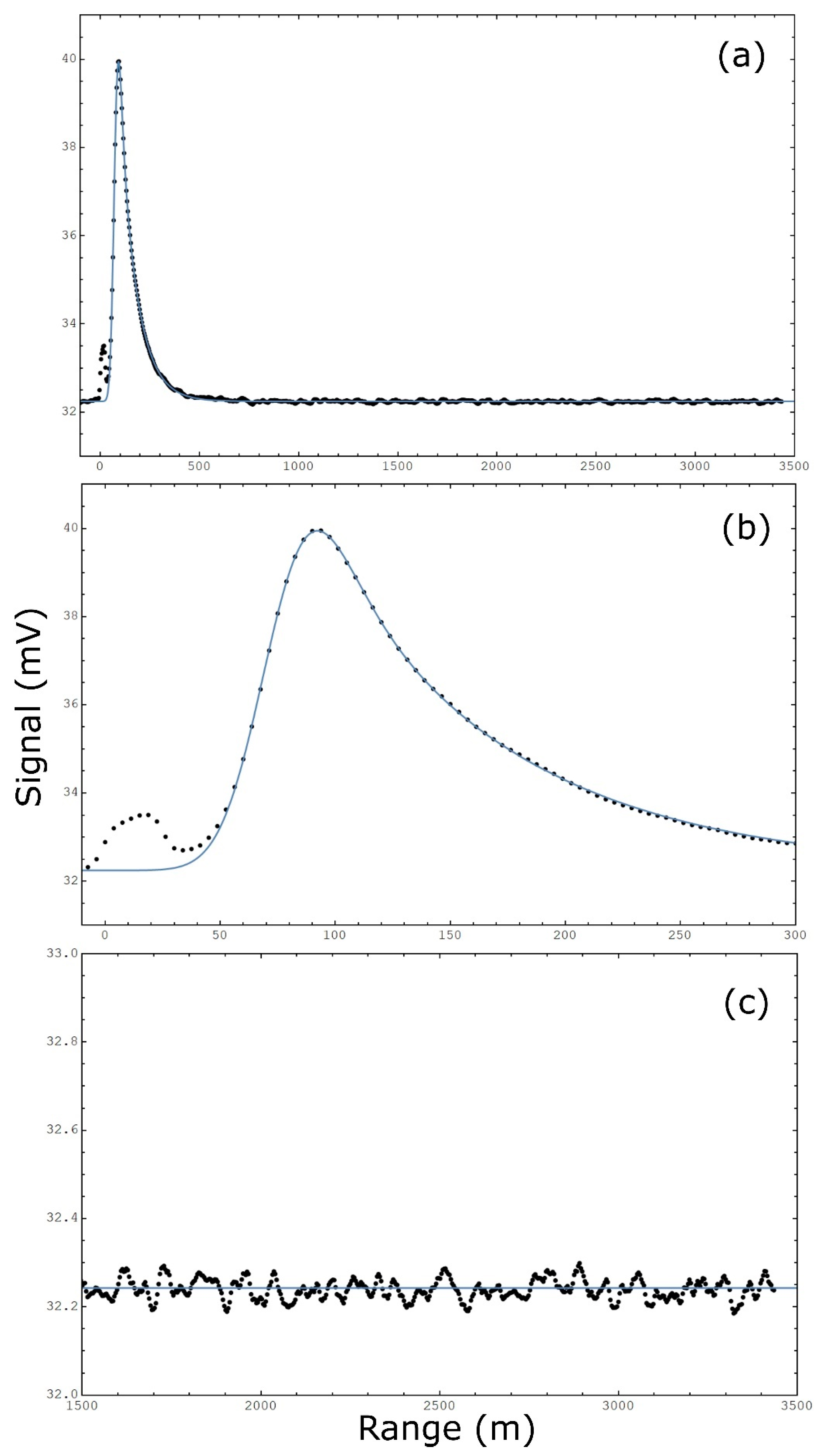
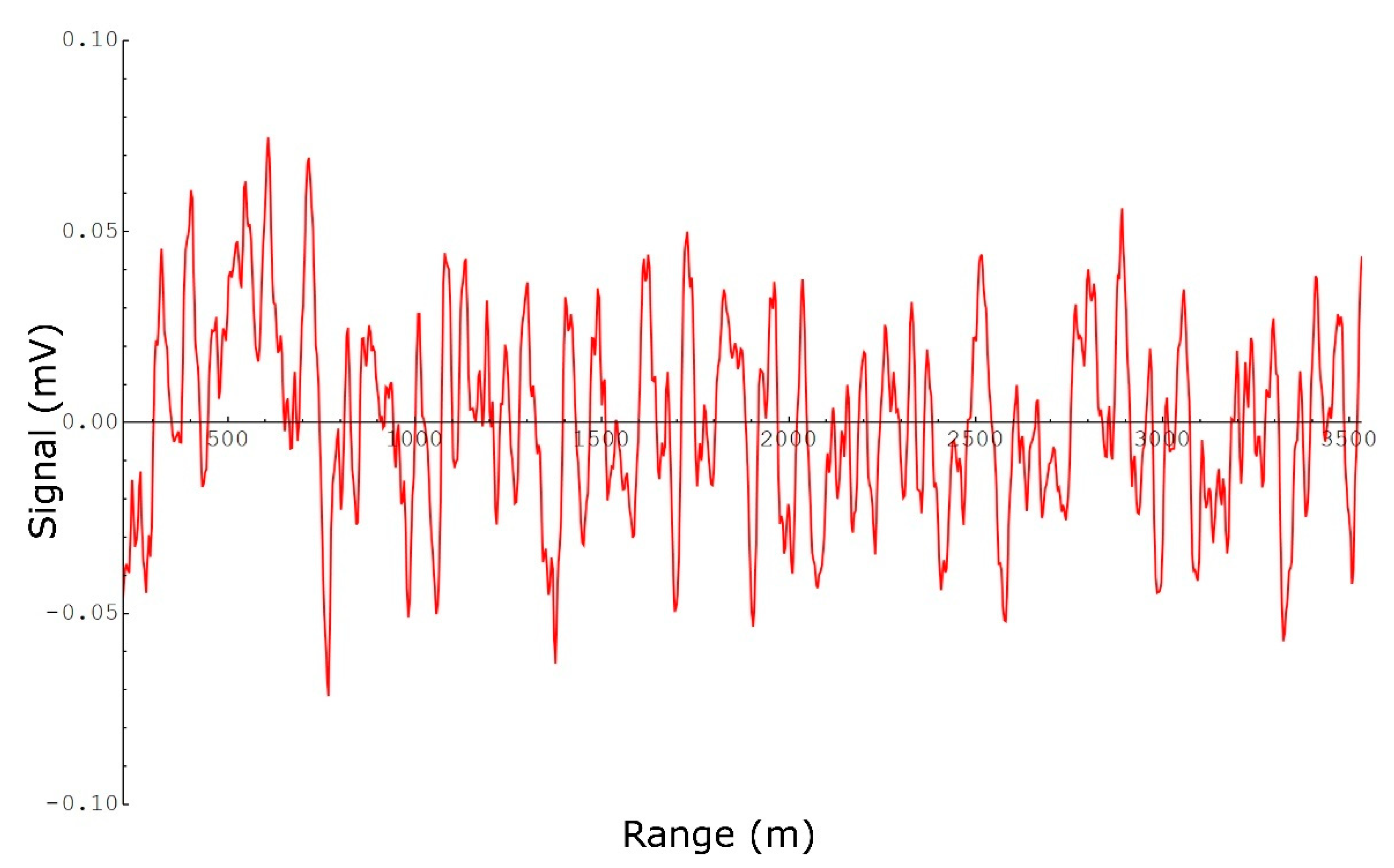
3.1. Determination of Uncertainty Sources

The values of the uncertainty sources in Equation (1) can be estimated from the experimental data. For the scanning line shown in Figure A1, the signal zero offset was calculated by averaging the data recorded from about 1700 to 3200 m from the DIAL. The standard uncertainties of the offsets u(o_on) and u(o_off) can be estimated by calculating the standard deviation of the mean of these datapoints; the uncertainty of the offset of the example scanning line was 1.0 µV. The standard uncertainties of the return signals u(f_on) and u(f_off) can be estimated by calculating the standard deviation of the detector noise in the region where the back-scatter signal is effectively zero, typically in the far-field at distances further than 1500 m, the same region where the offset is calculated. The assumptions are that the signal noise has a Gaussian-like distribution and that it is the same in the whole region, which is confirmed to be the case by the plots shown in Figure A2 and Figure A3. The noise uncertainty for the example signal was 22 µV, which is mainly dominated by the detector and amplifier noise averaged over n laser shots (250 in this example), but it also includes any other electrical noise in the system such as noise due to the transient digitiser. The standard uncertainties of the transmitted energies u(p_on) and u(p_off) can be estimated by calculating the standard deviation of the mean of a set of n pulses at constant energy. This is typically about 50–100 µV, 86 µV for the example scanning line, for energy readings that are typically in the 50–250 mV range. The methane Δα value used for this work is ~0.6 (ppm.km)⁻¹ with an uncertainty u_α defined in Equation (A3) of about 1.1%. The absorption coefficient and associated uncertainty were derived from the analysis of several calibration cell scans acquired over 15 years using reference gases with a traceable amount of methane. The ratio of the difference in the transmittance between the λ_on and λ_off wavelengths is recorded in each calibration scan of a reference gas concentration in a cell of a known length. From these values, it is possible to calculate for each scan a value of Δα. The average value used in this work was calculated from all the calibration cell scans analysed and the uncertainty was derived from the standard deviation of the mean of this set of scans.

3.2. Mass Emission Rate Uncertainty

The mass emission rate M(x) is calculated by combining the DIAL concentration measurements with the meteorological measurements as described in Equation (A35). The plane concentration C_plane measured within an area A of a vertical measurement plane using s scanning lines is defined in Equation (A32). Using the approximated Equation (A34) for the plane concentration uncertainty due to the DIAL system concentration measurement, u_sys(C_plane(x)), it is possible to rewrite the mass emission rate uncertainty due to the DIAL system concentration measurement u_sys(M(x)) defined in Equations (A40) as:

$$u_{sys}\left(M\left(x\right)\right)\cong \frac{u_{sys}\left(C\left(x\right)\right)}{\sqrt{s}}A v\sin \vartheta ,$$

(3)

where u_sys(C(x)) is defined in Equation (A15) as the system concentration uncertainty for a scanning line at a range x from the DIAL, v is the wind speed, and θ is the angle between the wind direction and the DIAL vertical measurement plane. It should be noted that the dependent variable x in Equation (3) is the range from the DIAL that defines the location of the plane, the region within which the concentration is determined. The size of the plane A is related to the sampling spacing l over which the concentration of each scanning line (s) is determined. Therefore, the uncertainty in M(x) is related to the region over which C(x) are determined.

As described in Section 2 and Appendix A, the targeted gas density must be added to Equation (3) in order to convert the concentration expressed in ppm to kg/m³ when the absorption coefficient unit used is (ppm km)⁻¹. The assumptions made in Equation (3), from Equation (A34), are that each of the s scanning lines is analysed in the same range l and each of them has a similar u_sys(C(x)) value. The former is typically correct when analysing the emission from a specific plume or targeted area while the latter assumption is reasonable since the same range l is analysed and both the detector signal uncertainty and signal return shapes are unlikely to change significantly over the period (10 to 15 min) a DIAL scan is recorded. The contribution of u_α is constant across the measured plane; it is proportional to M(x) and independent of the number of scanning lines s used in the scan. It can therefore be added in quadrature to u_sys(M(x)), which is independent from M(x), to calculate the total emission rate uncertainty due to the DIAL concentration measurement, u_c(M(x)) as shown in Equation (A39).

Typically, a DIAL scan is made up by a minimum of 7 scanning lines up to a maximum of 20, with s = 10 being a typical value. An example analysis spacing of l = 45 m can be chosen as a representative of a plume dimension typically observed with DIAL at industrial facilities. For simplicity, we can assume that such an emission plume was measured over an area A = 45 m × 45 m. To define a DIAL system performance and therefore be able to compare different DIAL systems and species measured, a fixed S/N value should be defined as a reference. In the DIAL system examined in this paper, an S/N better than 500 is achieved in favourable atmospheric conditions at a typical measurement range when averaging n = 250 laser shots. It should also be noted that an S/N = 500 can also be achieved in unfavourable atmospheric conditions by simply increasing the number laser shots n. The maximum value in the return signal shown in Figure A1 is at a distance x ~ 100 m from the DIAL. This value can be normalised so that its S/N = 500 and both f_on(x) and f_off(x) signals can then be normalised using the same factor.

Figure 1 shows u_c(M(x)) (red line) and u_sys(M(x)) (blue line) for an example 50 kg/h plume measured with l = 45 m, A = 45 m × 45 m, s = 10, v = 4 m/s, θ = 90°, and S/N = 500 at x ~ 100 m. The contribution of u_α to u_c(M(x)) is significant at distances from the DIAL where S/N is bigger and u_sys(M(x)) is smaller while it decreases at further distances from the DIAL since the intensity of the return DIAL signals decreases and u_sys(M(x)) becomes dominant. Equation (A39) shows that the impact of u_α is expected to decrease as the plume mass emission rate decreases. This is confirmed in Figure 2, where the contribution of u_α is negligible for a 15 kg/h plume as u_c(M(x))~u_sys(M(x)) through the whole range. The value of u_sys(M(x)) at x ~ 100 m from the DIAL where the S/N = 500 is ~0.6 kg/h and it is independent from the mass emission rate measured. However, this value depends on l and A, for example, it would decrease to ~0.3 kg/h if the plume was analysed with l = 30 m and A = 30 m × 30 m.

Figure 3 shows the uncertainty fractions u_sys(M(x))/M(x) (yellow line) and u_c(M(x))/M(x) (blue line) as a function of the plume mass emission rate measured at x ~ 100 m from the DIAL, where S/N = 500 for l = 45 m, A = 45 m × 45 m, s = 10, v = 4 m/s, and θ = 90°. For mass emission rates less than ~15 kg/h, u_sys(M(x)) is the dominant term while at higher emission rates, u_α becomes the dominant term in u_c(M(x)). In this exemplar case, a plume mass emission rate of 1.5 kg/h has an uncertainty fraction lower than 40%, which quickly decreases below 10% for mass emission rates higher than ~6 kg/h.

It should be noted the uncertainty plots reported will vary according to Equation (3) when using different values of l, A, s, v, and θ. Moreover, all the uncertainties reported here are from a DIAL scan, not a DIAL measurement, that is defined as the average emission rate measured from at least four DIAL scans. The uncertainty of a DIAL measurement and the impact of the uncertainties from the meteorological measurements as defined in Equation (A36) will be addressed in a follow-up paper.

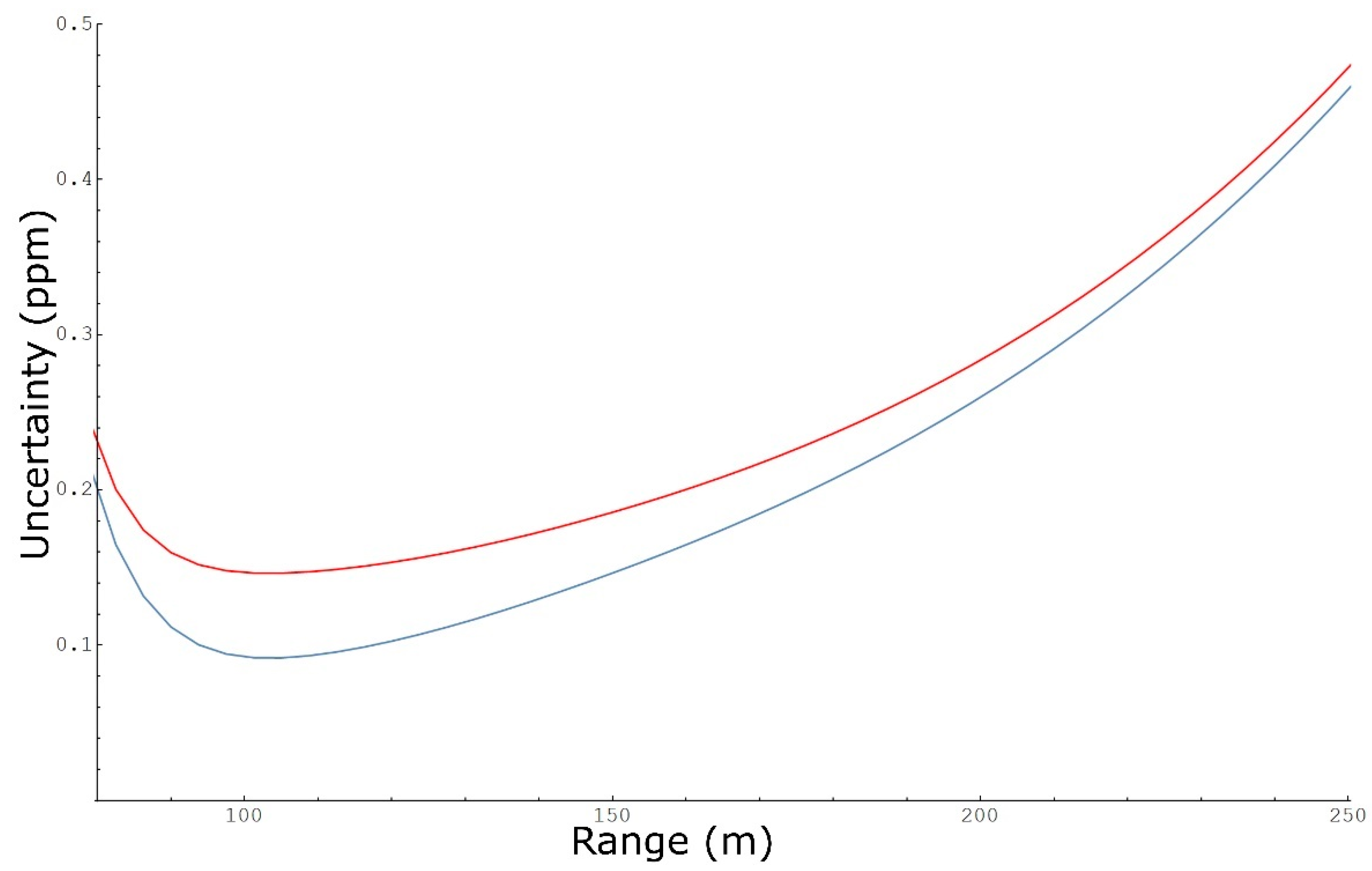
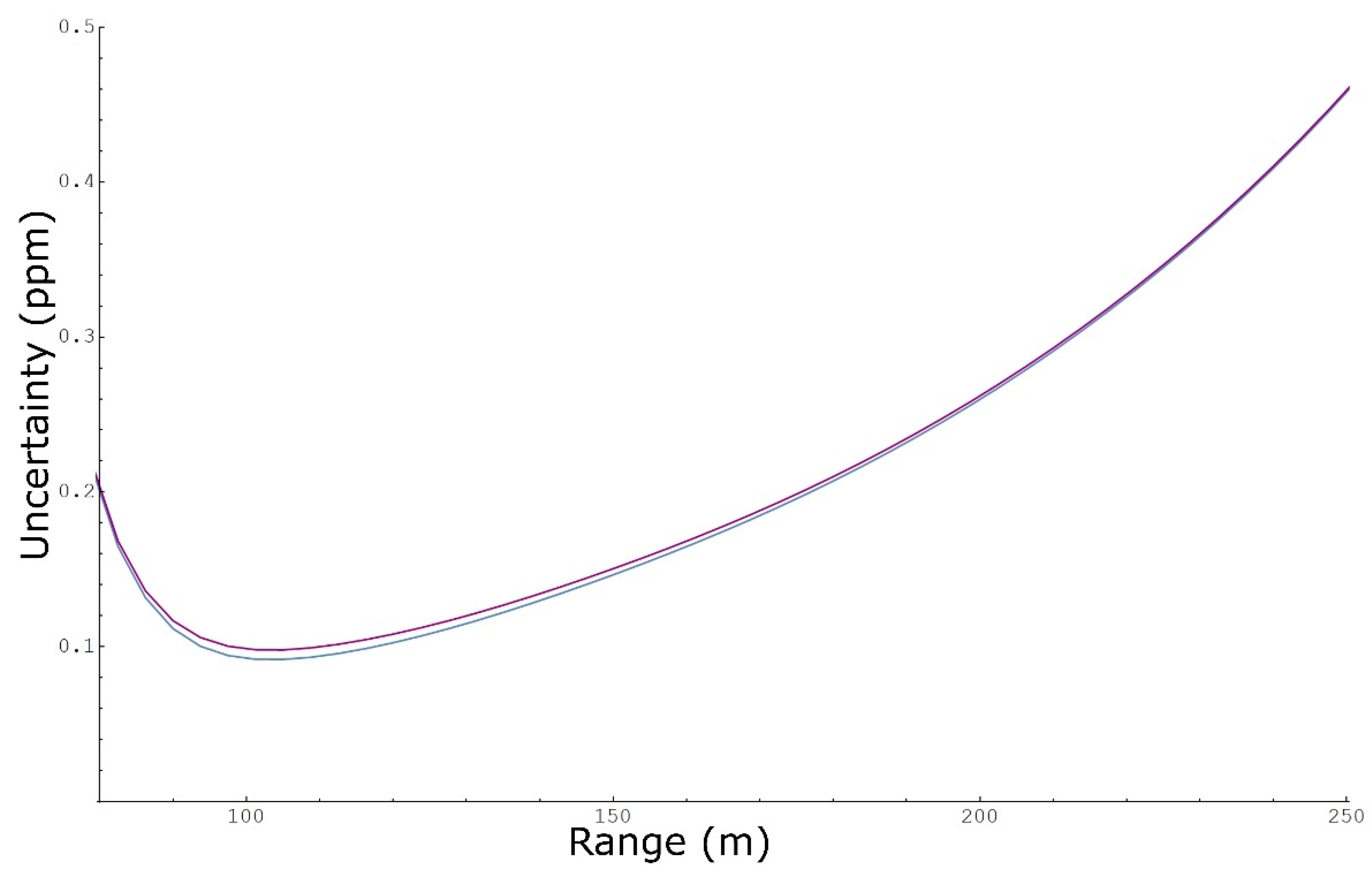
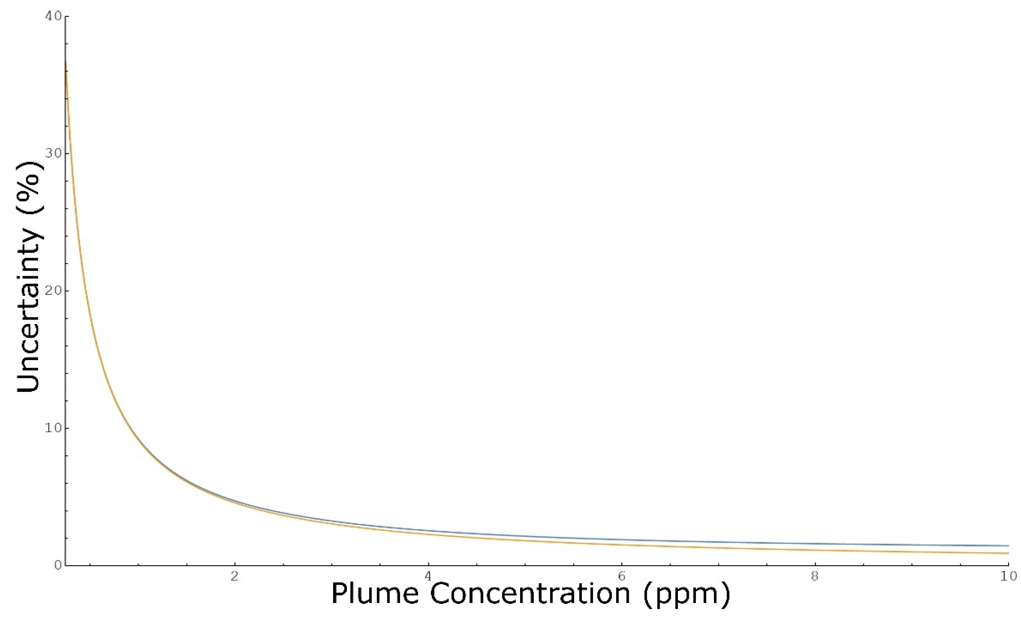
3.3. Concentration Uncertainty

The total concentration uncertainty u(C(x)) for a DIAL concentration measurement line s can be derived from Equation (A16):

$$u\left(C\left(x\right)\right)=\sqrt{u_{sys}{\left(C\left(x\right)\right)}^2+C{\left(x\right)}^2 {u_{\alpha }}^2}$$

(4)

The impact of u_α varies depending on the measured plume concentration and the distance of the centre of the plume from the DIAL as can be seen in Figure 4 and Figure 5. Figure 4 shows u(C(x)) (red line) and u_sys(C(x)) (blue line) for an example 10 ppm concentration plume measurement with l = 45 m and S/N = 500 at x ~ 100 m. The contribution of u_α to u(C(x)) is significant at distances from the DIAL where S/N is bigger and u_sys(C(x)) is smaller while it decreases at further distances from the DIAL since the intensity of the return DIAL signals decreases and u_sys(C(x)) becomes dominant. Equation (4) shows that the impact of u_α is expected to decrease as the concentration decreases. This is confirmed in Figure 5, where the contribution of u_α is negligible for the 3 ppm concentration plume as u(C(x))~u_sys(C(x)) through the whole range.

Figure 6 shows the concentration system uncertainty fraction u_sys(C(x))/C(x) (yellow line) and the concentration uncertainty fraction u(C(x))/C(x) (blue line) in the function of the plume concentration measured at x ~ 100 m from the DIAL where S/N = 500 for l = 45 m. For concentrations less than ~3 ppm, u_sys(C(x)) is the dominant term while at higher concentrations, u_α becomes the dominant term in u(C(x)). In this exemplar case, a plume concentration of 250 ppb has an uncertainty of about 35%, which quickly decreases below 10% for concentrations higher than ~1 ppm.

Figure 7 shows the contribution to the system uncertainty fraction u_sys(C(x))/C(x) reported in Equation (A23) of the four sources of uncertainty defined in Equations (A19) to (A22) calculated for l = 45 m. It is clear the signal uncertainties $u_{f_{on}}\left(C\left(x\right)\right)$ (purple line) and $u_{f_{off}}\left(C\left(x\right)\right)$ (light purple line) are the dominant terms when compared to the offset uncertainties $u_{o_{on}}\left(C\left(x\right)\right)$ (blue line) and $u_{o_{off}}\left(C\left(x\right)\right)$ (light blue line). Given the shape of the return signal in Figure A1, with the maximum signal intensity at 100 m, it is expected that the lower uncertainty is obtained when measuring a plume centred at about a 100 m distance from the DIAL. However, the shape and intensity of a DIAL return signal varies with the atmospheric (backscatter) conditions and by focusing the detection optics at shorter or longer distances from the DIAL. Therefore, the return signals (and uncertainty) can be optimised at different distances from DIAL depending on the location of the targeted measurement area.

For any DIAL system, it is important to assess the contribution of the offset uncertainties to u_sys(C(x)) to determine if they are negligible as in the case of this DIAL system. Equation (A25) describes u_sys(C(x)) as an approximation of Equation (A15) by ignoring the small contribution from the offset uncertainties. It is also reasonable to assume the on and off signal uncertainties defined in Equations (A26) and (A27) to be similar since these are dominated by the noise of the same detector. Another approximation could be made if the value of data points separated by the spacing l were similar, i.e., Equations (A28)–(A31), which is typically correct only for very small values of l. A further approximation can be made by assuming that the on and off signals are similar, i.e., Equations (A28)–(A31), which can be considered roughly valid only if the on and off laser beam powers were well balanced. With all these assumptions, Equation (A25) can be simplified to:

$$u_{sys}\left(C\left(x\right)\right)\cong \frac{1}{\mathsf{\Delta }\alpha l}\frac{N}{S},$$

(5)

which is the same equation reported by Fukuda et al. [16], assuming that the range dependence of the signal is not significant, i.e., the four terms in Equations (A25) are identical. In the case of the example scanning line used in this paper, the correct value of u_sys(C(x)) is 92 ppb when calculated using the full uncertainty analysis in Equation (A15) at x ~ 100 m from the DIAL where S/N = 500 for l = 45 m. If the approximated Equation (5) was used, u_sys(C(x)) would be calculated to be 74 ppb, which is about 20% lower than the correct value. The assumption that the range dependence of the signal is not significant is therefore incorrect as the approximation used to derive Equation (5) becomes worse for larger l values. The u_sys(C(x)) value is expected to decrease for measurements carried out over larger distances l while it increases for smaller l.

Equation (A15), or the approximate Equations (A25) and (5), could also be considered as representative of the minimum detectable concentration. It should be noted that some papers report a minimum detectable concentration equation that gives values that are exactly half of Equation (5) [17,18]. In these works, the minimum detectable concentration was derived from the DIAL path-concentration integral Equation (1) rather than the differential Equation (2) and therefore do not consider that uncertainties arise from both the start and end points of the selected range l. Moreover, the S/N value was only used once while both f_on(x) and f_off(x) signals have an associated uncertainty due to the detector S/N value. Essentially, only one of the four terms under the square root in Equation (A25) was considered, explaining the factor of two difference.

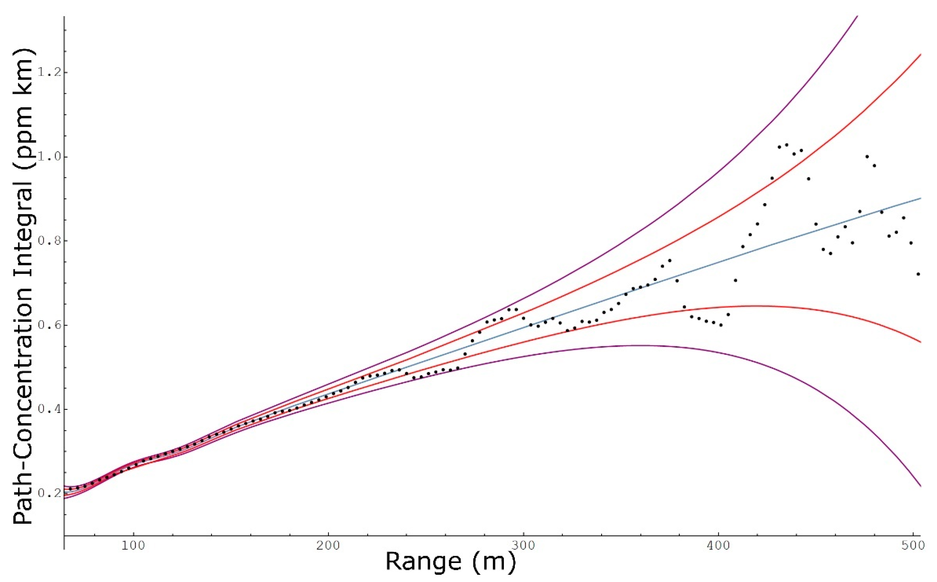
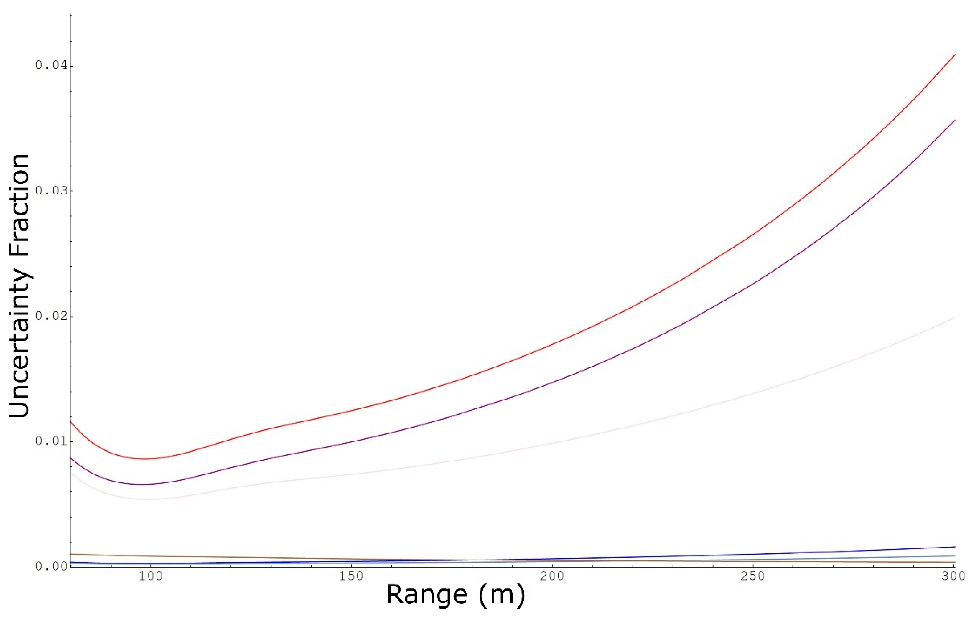
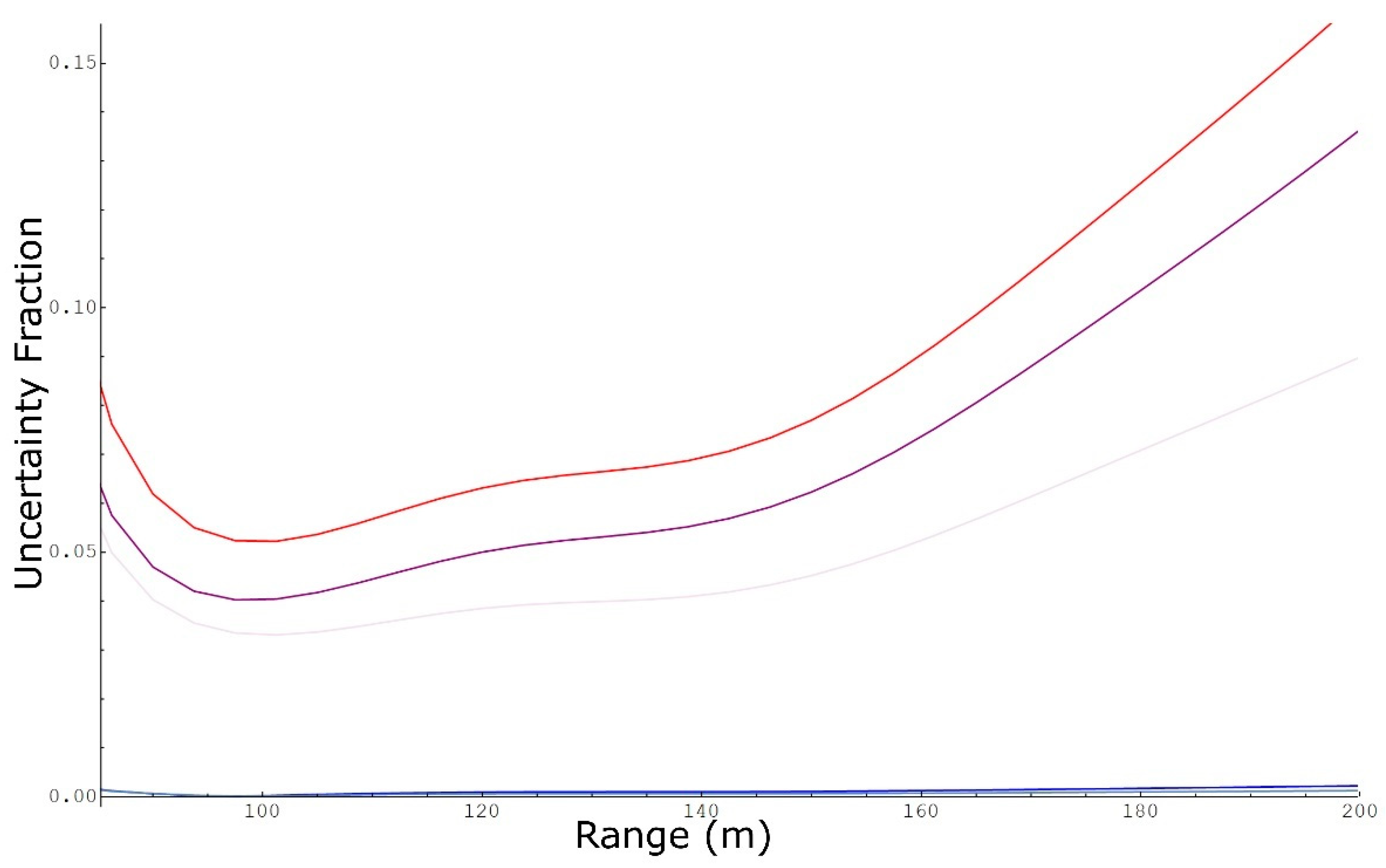
3.4. Path-Concentration Integral Uncertainty

The total uncertainty of a DIAL path-concentration integral u(CL(x)) and the system path-concentration integral uncertainty u_sys(CL(x)) are defined in Equations (A1) and (A2), respectively. The contribution of u_α can be added in quadrature to u_sys(CL(x)) as defined in Equation (A4) to calculate u(CL(x)). Figure 8 shows the CL(x) data points (black dots) for the example scanning line up to 500 m from the DIAL, CL(x) calculated by fitting the on and off return signals (blue line), CL(x) ± u_sys(CL(x)) (red lines) indicating the standard uncertainty, and CL(x) ± 2u_sys(CL(x)) (purple lines) providing a 95% level of confidence expanded uncertainty. The expanded uncertainty captures the variability of the data points from a straight line well, which represents the methane background concentration. Such an agreement indirectly confirms that the main uncertainty sources of a DIAL system can be derived from Equation (1) and that the assumptions made about these sources not being correlated was justifiable. In the case of the example scanning line used in this paper, the value of u_sys(CL(x)) is 2.3 ppb km at x ~ 100 m from the DIAL where S/N = 500.

Figure 9 shows the contribution to the integrated system uncertainty fraction u_sys(CL(x))/CL(x) reported in Equation (A11) of the six sources of uncertainty defined in Equations (A5) to (A10). It is clear the signal uncertainties $u_{f_{on}}\left(CL\left(x\right)\right)$ (purple line) and $u_{f_{off}}\left(CL\left(x\right)\right)$ (light purple line) are the dominant terms. The weight of the offset uncertainties $u_{o_{on}}\left(CL\left(x\right)\right)$ (blue line) and $u_{o_{off}}\left(CL\left(x\right)\right)$ (light blue line) increases at further distances from the DIAL, where the signals f_on(x) and f_off(x) decrease, when compared to the transmitted energy uncertainties $u_{p_{on}}\left(CL\left(x\right)\right)$ (yellow line) and $u_{p_{off}}\left(CL\left(x\right)\right)$ (light yellow line). As the signal uncertainties are the main uncertainty sources, it is clear the example scanning line presented here was optimised to measure sources located at a distance from the DIAL of about 80 m up to a maximum of about 300 m.

4. Discussion

For the example methane measurement presented in this work, the smaller uncertainty was obtained in the region where the return signal was higher, which was at about 100 m from the DIAL. At a representative S/N value of 500, the system methane concentration uncertainty for a concentration measurement over 45 m was calculated to be 92 ppb. The total concentration uncertainty can be calculated by adding the uncertainty from the absorption coefficient. This is negligible for concentrations lower than ~2 ppm, but given that the ambient methane concentration is around this level, the absorption coefficient uncertainty is often a significant contributor. However, the fractional uncertainty is higher at lower concentrations while it quickly decreases below 10% for concentrations higher than ~1 ppm.

Equations to calculate the mass emission rate uncertainty associated to a DIAL concentration scan through a vertical plane downwind of the targeted measurement area were also derived. For S/N = 500, s = 10, v = 4 m/s, and θ = 90°, the emission rate system uncertainty was calculated to be ~0.6 and ~0.3 kg/h for a methane plume measured over a 45 m × 45 m and 30 m × 30 m plane, respectively. The total mass emission rate uncertainty due to DIAL concentration measurement can be calculated by adding the uncertainty from the absorption coefficient, which is negligible for mass emission rates lower than ~15 kg/h while it becomes dominant for concentrations higher than ~15 kg/h for the methane absorption line used in this work. However, the fractional mass uncertainty is higher at lower mass emission rates, and it quickly decreases below 10% for mass emission rates higher than ~6 kg/h. The mass emission uncertainty for each DIAL concentration scan will vary depending on the actual analysis range, number of lines used in the analysis, and the meteorological conditions, and it can be evaluated numerically using Equation (3). This evaluation can either be carried out by including all the sources of uncertainties when evaluating the system concentration u_sys(C(x)) in Equation (A15) or using an underestimated value from Equation (5) as a rough approximation. for any S/N and l values as long as Δα is known for the targeted species.

It is possible to calculate the expected performances of the IR measurements of other species that use the same detection system and the same laser system, at similar wavelengths and energies, by normalising the methane value to the differential absorption coefficient of the targeted species. These conditions are satisfied for VOCs and ethane measurements that are regularly made with the NPL DIAL system. The mass emission rate uncertainty due to the DIAL system concentration measurement can also be calculated using Equation (3) by replacing the methane gas density with the gas density of either VOCs or ethane.

Table 1. Summary of methane, ethane, and VOCs u_sys(C(x)) values calculated at x ~ 100 m where S/N = 500 and l = 45 m and u_sys(M(x)) values calculated with l = 45 m (A = 45 m × 45 m) and l = 30 m (A = 30 m × 30 m) with s = 10, v = 4 m/s, and θ = 90°.

	l	Methane	Ethane	VOC	Units
usys(C(x))	45 m	92	22	37	ppb
usys(M(x))	45 m	0.6	0.3	1.1	kg/h
usys(M(x))	30 m	0.3	0.2	0.6	kg/h

shows the results of these calculations performed at x ~ 100 m from the DIAL where S/N = 500. The u_sys(C(x)) values are calculated for l = 45 m while two u_sys(M(x)) are reported for each species using l = 45 m (A = 45 m × 45 m) and l = 30 m (A = 30 m× 30 m) with s = 10, v = 4 m/s, and θ = 90°. As mentioned in Section 3.2, the u_sys(M(x)) values reported in Table 1 are representative of the mass emission rate uncertainties expected from the concentration measurement of a single DIAL scan, not from a DIAL measurement, which is the average of at least four DIAL scans. It is also possible to easily calculate the u_sys(M(x)) values for different values of s, v, and θ using Equation (3) by scaling the values in Table 1 to the different s, v, and θ values.

5. Conclusions

In this work we presented, for the first time, parametric functions of the DIAL path-concentration integral, concentration, and mass emission rates and their associated uncertainties. All of the seven sources of uncertainty of a DIAL concentration measurement of a target gas along a path line were assessed and propagated through each step of the data analysis to determine the mass emission rate uncertainty. The expanded uncertainty of the path-concentration integral captures the variability observed in the experimental data points well, confirming all uncertainty sources were correctly evaluated. The DIAL on and off signals are the dominant source of uncertainty for IR measurements by the NPL DIAL system, which are proportional to the detector S/N value. While the backscattered signal collected by the DIAL telescope can vary significantly during the day, based on the number of particles in the atmosphere, the main limiting factor for DIAL IR measurements is the noise performance of the IR detector. However, it is critical for any DIAL system to assess and control the contribution of the other sources of uncertainty to determine whether they are negligible when compared to the noise contribution of the detector in the relevant measurement ranges.

In the future, a full DIAL measurement uncertainty budget will be developed by adding the uncertainties from the meteorological measurements and considering the effect of averaging several DIAL scans when reporting a DIAL measurement.

References

1. Barthe, P.; Chaugny, M.; Roudier, S.; Delgado Sancho, L. Best Available Techniques (BAT) Reference Document for the Refining of Mineral Oil and Gas. Industrial Emissions Directive 2010/75/EU (Integrated Pollution Prevention and Control). Publ. Off. Eur. Union 2015. [Google Scholar]
2. CEN EN 17628. Available online: https://standards.cencenelec.eu/dyn/www/f?p=205:110:0::::FSP_PROJECT,FSP_LANG_ID:67021,25&cs=1499A1C530EC17BFF9D3EB0305EFECA18 (accessed on 24 March 2022).
3. Measures, R.M. Laser Remote Sensing: Fundamentals and Applications; Wiley: New York, NY, USA, 1984; ISBN 978-0-471-08193-7. [Google Scholar]
4. Milton, M.J.T.; Woods, P.T.; Jolliffe, B.W.; Swann, N.R.W.; McIlveen, T.J. Measurements of Toluene and Other Aromatic Hydrocarbons by Differential-Absorption LIDAR in the near-Ultraviolet. Appl. Phys. B 1992, 55, 41–45. [Google Scholar] [CrossRef]
5. Robinson, R.A.; Woods, P.T.; Milton, M.J.T. DIAL Measurements for Air Pollution and Fugitive-Loss Monitoring. In Proceedings of the Air Pollution and Visibility Measurements SPIE, Munich, Germany, 20 September 1995; Volume 2506, pp. 140–149. [Google Scholar]
6. Robinson, R.; Gardiner, T.; Innocenti, F.; Woods, P.; Coleman, M. Infrared Differential Absorption Lidar (DIAL) Measurements of Hydrocarbon Emissions. J. Environ. Monit. 2011, 13, 2213–2220. [Google Scholar] [CrossRef] [PubMed]
7. Innocenti, F.; Robinson, R.; Gardiner, T.; Finlayson, A.; Connor, A. Differential Absorption Lidar (DIAL) Measurements of Landfill Methane Emissions. Remote Sens. 2017, 9, 953. [Google Scholar] [CrossRef]
8. Byer, R.L.; Garbuny, M. Pollutant Detection by Absorption Using Mie Scattering and Topographic Targets as Retroreflectors. Appl. Opt. 1973, 12, 1496–1505. [Google Scholar] [CrossRef]
9. Schotland, R.M. Errors in the Lidar Measurement of Atmospheric Gases by Differential Absorption. J. Appl. Meteorol. 1974, 13, 71–77. [Google Scholar]
10. Browell, E.V. Differential Absorption Lidar Sensing of Ozone. Proc. IEEE 1989, 77, 419–432. [Google Scholar] [CrossRef]
11. Cao, N.; Fukuchi, T.; Fujii, T.; Collins, R.L.; Li, S.; Wang, Z.; Chen, Z. Error Analysis for NO2 DIAL Measurement in the Troposphere. Appl. Phys. B 2006, 82, 141–148. [Google Scholar] [CrossRef]
12. Cao, N.; Li, S.; Fukuchi, T.; Fujii, T.; Collins, R.L.; Wang, Z.; Chen, Z. Measurement of Tropospheric O3, SO2 and Aerosol from a Volcanic Emission Event Using New Multi-Wavelength Differential-Absorption Lidar Techniques. Appl. Phys. B 2006, 85, 163–167. [Google Scholar] [CrossRef]
13. Bösenberg, J. Ground-Based Differential Absorption Lidar for Water-Vapor and Temperature Profiling: Methodology. Appl. Opt. AO 1998, 37, 3845–3860. [Google Scholar] [CrossRef]
14. Wulfmeyer, V.; Bösenberg, J. Ground-Based Differential Absorption Lidar for Water-Vapor Profiling: Assessment of Accuracy, Resolution, and Meteorological Applications. Appl. Opt. AO 1998, 37, 3825–3844. [Google Scholar] [CrossRef] [PubMed]
15. Walmsley, H.L.; O’Connor, S.J. The Accuracy and Sensitivity of Infrared Differential Absorption Lidar Measurements of Hydrocarbon Emissions from Process Units. Pure Appl. Opt. 1998, 7, 907–925. [Google Scholar] [CrossRef]
16. Fukuda, T.; Matsuura, Y.; Mori, T. Sensitivity of Coherent Rage-Resolved Differential Absorption Lidar. Appl. Opt. AO 1984, 23, 2026–2032. [Google Scholar] [CrossRef] [PubMed]
17. Veerabuthiran, S.; Razdan, A.K. LIDAR for Detection of Chemical and Biological Warfare Agents. Def. Sci. J. 2011, 61, 241–250. [Google Scholar] [CrossRef]
18. Veerabuthiran, S.; Razdan, A.K.; Jindal, M.K.; Prasad, G. Open Field Testing of Mid IR DIAL for Remote Detection of Thiodiglycol Vapor Plumes in the Topographic Target Configuration. Sens. Actuators B Chem. 2019, 298, 126833. [Google Scholar] [CrossRef]
19. Gong, Y.; Bu, L.; Yang, B.; Mustafa, F. High Repetition Rate Mid-Infrared Differential Absorption Lidar for Atmospheric Pollution Detection. Sensor 2020, 20, 2211. [Google Scholar] [CrossRef]
20. Menyuk, N.; Killinger, D.K.; Menyuk, C.R. Error Reduction in Laser Remote Sensing: Combined Effects of Cross Correlation and Signal Averaging. Appl. Opt. AO 1985, 24, 118–131. [Google Scholar] [CrossRef]
21. Milton, M.J.; Woods, P.T. Pulse Averaging Methods for a Laser Remote Monitoring System Using Atmospheric Backscatter. Appl. Opt. 1987, 26, 2598–2603. [Google Scholar] [CrossRef]
22. Grant, W.B.; Brothers, A.M.; Bogan, J.R. Differential Absorption Lidar Signal Averaging. Appl. Opt. 1988, 27, 1934–1938. [Google Scholar] [CrossRef]
23. Lindström, T.; Holst, U.; Weibring, P.; Edner, H. Analysis of Lidar Measurements Using Nonparametric Kernel Regression Methods. Appl. Phys. B 2002, 74, 155–165. [Google Scholar] [CrossRef]
24. Lindström, T.; Holst, U.; Weibring, P. Analysis of Lidar Fields Using Local Polynomial Regression. Environmetrics 2005, 16, 619–634. [Google Scholar] [CrossRef]
25. Innocenti, F.; Robinson, R.; Gardiner, T.; Howes, N.; Yarrow, N. Results from a Global Study Measuring Methane Emissions from Onshore LNG Facilities Using Differential Absorption Lidar (DIAL). in press.
26. Bourn, M.; Robinson, R.; Innocenti, F.; Scheutz, C. Regulating Landfills Using Measured Methane Emissions: An English Perspective. Waste Manag. 2019, 87, 860–869. [Google Scholar] [CrossRef] [PubMed]
27. United Nations the Paris Agreement. Available online: https://www.un.org/en/climatechange/paris-agreement (accessed on 24 March 2022).
28. Global Methane Pledge. Available online: https://www.globalmethanepledge.org/ (accessed on 24 March 2022).
29. Oil and Gas Methane Partnership (OGMP) 2.0 Framework. Available online: https://www.ccacoalition.org/en/resources/oil-and-gas-methane-partnership-ogmp-20-framework (accessed on 24 March 2022).
30. Howes, N.; Finlayson, A.; Smith, T.; Innocenti, F.; Robinson, R.A. Final Report on cen/tc264/wg38 Stationary Source Emissions—Standard Method to Determine Fugitive and Diffuse Emissions of Volatile Organic Compounds in the Atmosphere. Available online: https://www.vdi.de/fileadmin/pages/vdi_de/redakteure/ueber_uns/fachgesellschaften/KRdL/dateien/WG_38_Final_Report_SACEN2014-07.pdf (accessed on 24 March 2022).
31. Babilotte, A.; Lagier, T.; Fiani, E.; Taramini, V. Fugitive Methane Emissions from Landfills: Field Comparison of Five Methods on a French Landfill. J. Environ. Eng.-ASCE 2010, 136, 777–784. [Google Scholar] [CrossRef]
32. Babilotte Field Intercomparisons of Methods to Measure Fugitive Methane Emissions. Available online: https://erefdn.org/field-intercomparisons-of-methods-to-measure-fugitive-methane-emissions/ (accessed on 24 March 2022).
33. Pikelnaya, O.; Polidori, A.; Tisopulos, L. Controlled Release. Available online: http://www.aqmd.gov/ors-study/controlled-release (accessed on 24 March 2022).
34. Gardiner, T.; Helmore, J.; Innocenti, F.; Robinson, R. Field Validation of Remote Sensing Methane Emission Measurements. Remote Sens. 2017, 9, 956. [Google Scholar] [CrossRef]
35. Rye, B.J. Differential Absorption Lidar System Sensitivity with Heterodyne Reception. Appl. Opt. AO 1978, 17, 3862–3864. [Google Scholar] [CrossRef]
Figure 1. usys(M(x)) (blue line) and uc(M(x)) (red line) for a 50 kg/h plume up to 250 m from the DIAL for l = 45 m, A = 45 m × 45 m, s = 10, v = 4 m/s and θ = 90°, and S/N = 500 at x ~ 100 m. Note that the range starts at x ~ 80 m since this is equivalent, for l = 45 m, to starting the analysis just after the near field backscatter light at ~60 m distance from the DIAL (xl/2).
Remotesensing 14 04291 g001
Figure 2. usys(M(x)) (blue line) and uc(M(x)) (purple line) for a 15 kg/h plume up to 250 m from the DIAL for l = 45 m, A = 45 m × 45 m, s = 10, v = 4 m/s and θ = 90°, and S/N = 500 at x ~ 100 m.
Remotesensing 14 04291 g002
Figure 3. usys(M(x))/M(x) (yellow line) and uc(M(x))/M(x) (blue line) in the function of the plume mass emission rate centred at x ~ 100 m from the DIAL (S/N = 500) for l = 45 m, A = 45 m × 45 m, s = 10, v = 4 m/s, and θ = 90°.
Remotesensing 14 04291 g003
Figure 4. usys(C(x)) (blue line) and u(C(x)) (red line) for the 10 ppm concentration plume up to 250 m from the DIAL for l = 45 m and S/N = 500 at x ~ 100 m.
Remotesensing 14 04291 g004
Figure 5. usys(C(x)) (blue line) and u(C(x)) (purple line) for the 3 ppm concentration plume up to 250 m from the DIAL for l = 45 m and S/N = 500 at x ~ 100 m.
Remotesensing 14 04291 g005
Figure 6. usys(C(x))/C(x) (yellow line) and u(C(x))/C(x) (blue line) in the function of the plume concentration centred at x ~ 100 m from the DIAL (S/N = 500) for l = 45 m.
Remotesensing 14 04291 g006
Figure 7. usys(C(x))/C(x) (red line) up to 200 m from the DIAL and the contributing terms as shown in Equation (A23): u f o n ( C ( x ) ) (purple line), u f o f f ( C ( x ) ) (light purple line),   u o o n ( C ( x ) ) (blue line), and u o o f f ( C ( x ) ) (light blue line) calculated for l = 45 m and S/N = 500 at x ~ 100 m.
Remotesensing 14 04291 g007
Figure 8. CL(x) data points (black dots) up to 500 m from the DIAL, CL(x) fit (blue line), CL(x) ± usys(CL(x)) (red lines), and CL(x) ±2usys(CL(x)) (purple lines).
Remotesensing 14 04291 g008
Figure 9. usys(CL(x))/CL(x) (red line) up to 300 m from the DIAL and the contributing terms as shown in Equation (A11): u f o n ( C L ( x ) ) (purple line), u f o f f ( C L ( x ) ) (light purple line), u o o n ( C L ( x ) )   ( b l u e   l i n e ) ,   u o o f f ( C L ( x ) )   ( l i g t h t   b l u e   l i n e ) , u p o n ( C L ( x ) ) (yellow line), and u p o f f ( C L ( x ) ) (light yellow line overlapping with the yellow line).
Remotesensing 14 04291 g009