Article

Sentinel-1 Shadows Used to Quantify Canopy Loss from Selective Logging in Gabon

1
School of GeoSciences, The University of Edinburgh, Edinburgh EH8 3FF, UK
2
Rougier Gabon, Immeuble Le Narval, Libreville, Gabon
3
Department of Geography, Omar Bongo University, Libreville, Gabon
4
Agence Gabonaise d’Etudes et d’Observations Spatiales, Libreville, Gabon
5
Department of Geography, University College London, London WC1E 6BT, UK
*
Author to whom correspondence should be addressed.
Remote Sens. 2022, 14(17), 4233; https://doi.org/10.3390/rs14174233
Submission received: 27 April 2022 / Revised: 18 August 2022 / Accepted: 19 August 2022 / Published: 27 August 2022

Abstract

:
Selective logging is a major cause of forest degradation in the tropics, but its precise scale, location and timing are not known as wide-area, automated remote sensing methods are not yet available at this scale. This limits the abilities of governments to police illegal logging, or monitor (and thus receive payments for) reductions in degradation. Sentinel-1, a C-band Synthetic Aperture Radar satellite mission with a 12-day repeat time across the tropics, is a promising tool for this due to the known appearance of shadows in images where canopy trees are removed. However, previous work has relied on optical satellite data for calibration and validation, which has inherent uncertainties, leaving unanswered questions about the minimum magnitude and area of canopy loss this method can detect. Here, we use a novel bi-temporal LiDAR dataset in a forest degradation experiment in Gabon to show that canopy gaps as small as 0.02 ha (two 10 m × 10 m pixels) can be detected by Sentinel-1. The accuracy of our algorithm was highest when using a timeseries of 50 images over 20 months and no multilooking. With these parameters, canopy gaps in our study site were detected with a false alarm rate of 6.2%, a missed detection rate of 12.2%, and were assigned disturbance dates that were a good qualitative match to logging records. The presence of geolocation errors and false alarms makes this method unsuitable for confirming individual disturbances. However, we found a linear relationship ( r 2 = 0.74 ) between the area of detected Sentinel-1 shadow and LiDAR-based canopy loss at a scale of 1 hectare. By applying our method to three years’ worth of imagery over Gabon, we produce the first national scale map of small-magnitude canopy cover loss. We estimate a total gross canopy cover loss of 0.31 Mha, or 1.3% of Gabon’s forested area, which is a far larger area of change than shown in currently available forest loss alert systems using Landsat (0.022 Mha) and Sentinel-1 (0.019 Mha). Our results, which are made accessible through Google Earth Engine, suggest that this approach could be used to quantify the magnitude and timing of degradation more widely across tropical forests.

1. Introduction

There is an urgent need to accurately map and quantify forest degradation—which we define as a localised loss of aboveground biomass (AGB) not big enough to result in conversion to a non-forest state—across the tropics. This is for a number of reasons. Firstly, as tropical forests transition under climate change to net carbon sources [1,2,3,4] and towards potential ecosystem tipping points [5,6,7,8], a full picture of disturbance patterns will help to constrain the global carbon budget [3]. Secondly, in some places, degradation is a precursor to deforestation [9], so an ability to detect it could potentially prevent future forest loss. Thirdly, degradation involves the loss of carbon to the atmosphere and a reduction in forest resilience to future disturbance events such as drought [3,10]. Finally, degradation (and to a greater extent subsequent deforestation) has significant negative impacts on biodiversity [11,12,13]. Degradation maps will therefore help to quantify concerns about extinction rates [14,15] and to target measures aimed at protecting the high diversity of life found in tropical forest ecosystems [16,17]. The tropics have experienced, and are experiencing, rapid rates of land use change [18,19,20] as they are an important source of timber, rubber, minerals and food products to the world economy [21,22,23,24]. There are pledges to halt and reverse deforestation and forest degradation made by nations as part of their Paris Agreement commitments, including plans by developed countries to fund this transition [25]. However, in order to achieve this, robust, verifiable and unbiased forest monitoring techniques must be made widely available to enable the targeting and monitoring of pledges and funds [26,27].
The Sentinel-1 (S-1) mission funded by the European Union and operated by the European Space Agency (ESA) is a promising tool for pantropical forest monitoring as it provides regular, reliable and high resolution imagery over the entire tropical landmass. The acquisition plan of S-1 is optimised for wide area coverage and guarantees a 12 day revisit period even when one of the two satellites is out of operation [28]. A third and fourth satellite are planned and funded, which would ensure continuity of data beyond 2030 [29], ensuring consistent forest monitoring into the future. Unlike optical wavelengths, the C-band synthetic aperture radar (SAR) of S-1 can see through cloud and is only slightly attenuated by even heavy rain, meaning that practically every image contains useful data on the Earth’s surface [30]. This is especially important in the tropics, which include many of the cloudiest terrestrial regions on Earth [31]. The resulting dense time series is ideal for change detection as it allows high frequency changes (such as a sudden logging event) to be resolved [32,33,34]. S-1 also has high spatial resolution (range resolution 3 m and an azimuth resolution 20 m in the most commonly used interferometric wide-swath mode [29]), a further advantage in degradation mapping as individual disturbances are often small in scale: in this paper, we will show many logging disturbances are as small as 0.01 ha (10 m × 10 m). Finally, the open access data policy of S-1 and its availability on easy-to-use cloud platforms such as Google Earth Engine (GEE) and Microsoft’s Planetary Computer lend themselves to transparent, verifiable (repeatable) analyses, suiting both the scientific community and end users.
A growing body of work has demonstrated the potential of S-1 in tropical forests, including applications such as land cover mapping [35,36] and deforestation detection [37,38,39]. In particular, a number of publications have focused on wide area mapping of forest disturbances, much of this work stemming from the demonstration by Bouvet et al. [40] in 2018 that a S-1 shadowing effect can be used to detect patches of forest loss. An important observation in that study is that the backscattering properties of deforested land may not be significantly different to that of forest, especially once regrowth is underway, but a more robust feature exists at the boundary between tall trees and an area that has been cut. Here, there is a sudden change in height of the scattering surface. In places where this change has a negative component in the range direction of a radar satellite, there exists a SAR shadow, that is, a region where no backscatter can return to the sensor.
The S-1 shadow effect was initially used to reconstruct patches of deforestation in the Peruvian Amazon, and was estimated to have a detection rate of 95% for patches greater than 0.4 ha [40]. This result compared favourably to the University of Maryland (UMD) forest alert system [41]: a platform widely regarded as the benchmark in terms of global deforestation detection, but limited by the coarser pixel size (30 m, or 0.09 ha) and inability to penetrate the clouds with the Landsat sensors it relies on for raw data. The possibility of near real time (NRT) monitoring regardless of cloud cover, for example during the wet season in the Congo Basin, led to further research aimed at delivering short latency disturbance alert using Sentinel-1.
Hoekman et al. laid down a framework for detecting the emergence of very small features such as canopy gaps from selective logging, roads and canals [42]. The authors highlight the fact that radar detects changes in forest structure—a more stable and reliable metric than spectral features which quickly disappear due to regrowth [43]. Additionally, Hoekman et al. used a physical model to suggest a relationship between S-1 shadows and upper canopy loss: a relationship which we test empirically in this paper.
Stemming from the methods of [40,42], large scale forest disturbance alert maps began to be published around the year 2020. This included maps in Gabon [44], French Guiana [45], Vietnam, Laos and Cambodia [46,47] using a processing chain developed by the French National Centre for Space Studies (CNES) and the Center for the Study of the Biosphere from Space (CESBIO). An alternative algorithm implemented in GEE was used by Reiche et al. to generate the Radar for Detecting Deforestation (RADD) alert system, which now covers both the Congo and Amazon basins [48]. The main difference between the two approaches is that CESBIO determines shadows by identifying pixels where a radar change ratio (RCR) exceeds a certain threshold, while the RADD algorithm applies a Bayesian method to estimate the probability of change in a pixel [49]. However, both methods are underpinned by the shadow effect to some degree, and both use object level analysis to combine pixels and provide timely alerts with low false alarm rates (2–9%).
The principal limitation of previous work has been a reliance on optical satellite data for calibration and validation. For example, ref. [40] uses Sentinel-2 images to identify disturbances; ref. [42] relies primarily on Sentinel-2 and Google Earth imagery; ref. [45] uses manually interpreted SPOT, Pleiades, Landsat and Sentinel-2 data; ref. [48] uses PlanetScope mosaics; and ref. [46] relies on Google Earth and Planet optical images as reference data. In every case, the reference data have inherent and unknown uncertainty about how it relates to the true amount and location of degradation, particularly with respect to its missed detection rate for smaller disturbances. This has therefore made it so far impossible to determine the minimum size of disturbance detectable by S-1 or to test its ability to map a physical quantity of forest disturbance such as gross canopy cover loss. This is not to understate the important of such NRT alert systems, which clearly mark a considerable advance in the detection of tropical forest disturbance, but only to highlight that further work is required to develop maps that quantify the full extent and magnitude of degradation, through the use of reference data with known accuracy down to the finest scales.
Here, we use two unoccupied aerial vehicle (UAV) LiDAR acquisitions separated by approximately 1 year, collected over a logging concession in Gabon with experimental plots where controlled different levels of trees were removed, and changes occurred in a less controlled manner in the surrounding area [50]. This dataset, with known and varied changes in canopy cover, enabled us to overcome the limitations of using satellite images as reference data. This allows us to assess a S-1 algorithm against extremely precise (centimetre precision) measurements of forest height and structural change [51,52]. Such measurements leave negligible uncertainty in the location and size of canopy gaps as small as individual ground range detected (GRD) S-1 pixels (0.01 ha), making it possible for the first time to validate disturbances down to the scale of individual tree crowns. Furthermore, it enables us to test for a relationship between canopy cover loss and S-1 shadows.
In comparing S-1 shadows to UAV LiDAR, we posed the following hypotheses: (1) that S-1 would be capable of detecting canopy gaps caused by selective logging of individual large trees; (2) that the best accuracy for such a detection algorithm would be obtained by combining a long time series and avoiding spatial averaging; and (3) that a linear relationship would exist between the area of detected S-1 shadow and gross canopy loss due to selective logging. The aim of this paper was firstly to test these three hypotheses, and then to demonstrate the potential of S-1 degradation mapping if NRT capability is forgone for the sake of spatial resolution by estimating gross canopy cover loss and area of human disturbance in all forested areas of Gabon for the year 2020.

2. Materials and Methods
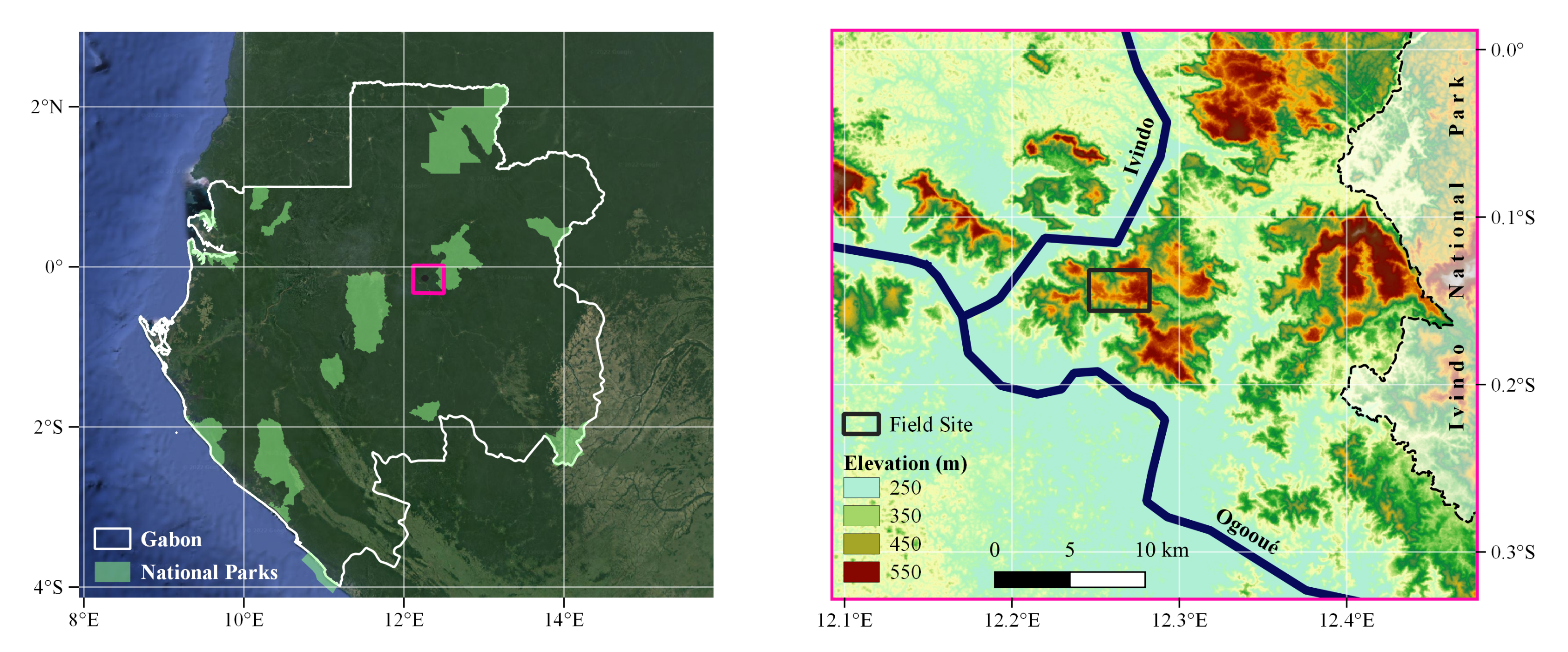
2.1. Field Site

Our study site is located in the Rougier-Gabon licensed logging concession in the Ogooué-Ivindo department of Gabon (Figure 1) at a disused airstrip around 9 km from Ivindo train station and village. Apart from the airstrip and adjoining access roads, the site is forested. Field surveys of four 1-ha plots found stem densities of 271 to 366 ha−1 and an average biomass density of 470 Mg ha−1 [53], which fits the general profile of African tropical forests as low turnover and high biomass compared to those in the majority of Latin American forests [54]. The region has a climate consisting of two dry seasons running from June to September and December to February, frequent low-lying cloud [55] and annual precipitation of less than 2000 mm. Satellite measurements [56] and nearby ground data [57] show a drying and warming of the climate over the last few decades.
Logging operations in the area are certified by the Forest Stewardship Council (FSC-C144419) and managed by Rougier Gabon, who fell Okoumé (Aucoumea klaineana) and other approved species for commercial timber. With permission from Gabon’s Ministry for the Protection of the Environment and Natural Resources, Forests and the Seas, a controlled logging experiment took place between 24 January and 28 January 2020 in which a total of 18 trees were felled according to low-impact logging practices in our four measured plots, resulting in aboveground biomass losses ranging from 7% to 23% per ha [53]. The area around the airstrip was later selectively logged as part of Rougier Gabon’s approved extraction program between November 2020 and January 2021.

2.2. UAV LiDAR

UAV LiDAR data were obtained between 16 January and 23 January 2020 (prior to the logging experiment) and again between 18 January and 21 January 2021 (after widespread selective logging had occurred). A DELAIR DT26X fixed-wing UAV was flown at 110 m altitude at an average speed of 17 ms−1 and loaded with a RIEGL miniVUX-1DL discrete-return LiDAR, yielding a point density of 240 pts m−2. Following post-processing kinematic correction, the geometric accuracy for both campaigns was estimated to be 1.8 cm based on ground control points [50]. Top Canopy Height (TCH) was defined as the difference between the lowest and highest returns in 25 cm cells after filtering for noise [50].
The change in TCH between the two field campaigns (Figure 2) was used to determine the precise location and geometry of new canopy gaps. Areas of undergrowth clearance were excluded and gaps were defined as spatially connected regions greater than 0.01 ha where TCH decreased by 10 m or more. In total, 261 canopy gaps were identified as having appeared between the two field campaigns, covering 5.2% of the 310 ha analysed.

2.3. Sentinel-1 Shadow Detection

Our algorithm follows the principle that where a tree crown disappears by anthropogenic or natural causes, the reflective (to C-band SAR) surface of its upper branches and leaves is replaced by a space devoid of radar scattering surfaces. Furthermore, the side looking geometry of SAR and considerable height of most tropical forests mean that the ground below the resulting canopy gap is shielded from the view of the sensor [40]. We therefore expect a sudden, localised decrease in backscatter that is sustained for a long period (at least while regrowth is confined to the understorey) and independent of absolute backscatter.
Importantly, we note that, in addition to the emergence of this shadow, a canopy gap leads to a region of increased radar brightness caused by radar overlay at the far range edge of the gap [42]. In the case of very small canopy gaps, for example those caused by the felling of an individual tree, the distance between the shadow and layover may approach the sensor resolution. At this point, any spatial averaging of backscatter will therefore risk destroying the disturbance signal as the two effects cancel each other out. To solve this issue and detect the smallest possible disturbances, we minimised spatial multilooking and instead used temporal averaging to mitigate speckle. This approach relies on our assumption that the shadow signal might be at the limit of what is detectable at SAR resolution over random noise, but persists for long enough that it will be visible in a large number of post disturbance images, enabling the signal to be visible over the noise.
Building on the methods of [40,45,46], we quantified shadow emergence through a radar change ratio (RCR) [58]. Our approach differed in that we made use of multiple polarisations where previous studies tended to use VV only; analysed longer time series of images after disturbance events compared to previous work that prioritised near real-time capability; and adopted a purely pixel-based algorithm as opposed to reconstructing forest loss patches as objects. To classify a pixel as shadow at time t in a sequence of images separated by repeat period Δ t , we required that the backscatter σ in the n images after t showed a significant decrease compared to the m previous images in both VV and VH polarisations. Explicitly, pixels meeting the following condition were flagged as potential shadows:
max ( RCR V V + α ) , 0 · max ( RCR V H + α ) , 0 > α 2
where
RCR p o l ( t ) = 1 n t t + n Δ t σ p o l ( t ) 1 m t m Δ t t σ p o l ( t )
and α is a threshold parameter determining how large a decrease in backscatter is required. Equations (1) and (2) are given for σ in decibels, which is why the RCR is expressed as a difference, and it assumed that there is no image exactly at time t.
We applied this algorithm to dual polarisation SAR images captured by ESA’s Sentinel-1A satellite, obtained through GEE in ground range detected (GRD) format with a pixel spacing of 10 m (equivalent number of looks of 4.3). As dictated by availability over Gabon, all images were taken on descending passes with Δ t equal to 12 days. Apart from two acquisitions found to be corrupted by signal interference on 31 January 2021, all data between December 2018 and December 2021 in the 15 scenes intersecting Gabon were used, totalling 1363 images. The imagery supplied by GEE was already calibrated for thermal noise and corrected for geometric distortions using the 30 m SRTM digital elevation model [59,60].
An advantage to using a change ratio is that the effects of terrain on the magnitude of backscatter do not need to be corrected for, as shadow detections are triggered by a relative decrease. As such, no additional pre-processing was applied to the S-1 images, apart from an optional multilooking step using a 3 × 3 spatial window (equivalent number of looks 38.7).
The condition in Equation (1) was tested for values of t every 12 days between December 2019 and February 2021. For every pixel that met the condition for at least one value of t, the value of t for which the left-hand side of Equation (1) was greatest (i.e., the point showing the largest decrease) was assigned as the most likely disturbance date, and where this fell outside of the time between the UAV acquisitions when comparing to the LiDAR data or the year 2020 when creating an annual product, the shadows were discarded. The remaining flagged pixels were then confirmed as shadow if they connected to at least one other shadow pixel.
Finally, non-forested areas were masked using ESA’s WorldCover 2020 product, a 10 m resolution global land cover map based on Sentinel-1 and Sentinel-2 data [61]. As such, forest is defined in our results as an area dominated by trees with at least 10% canopy cover [62]. This step was performed after filtering out single-pixel shadows to avoid missed detections around forest edges such as road expansion and new logging bays.

2.4. Accuracy Assessment

The optimum parameters for canopy cover loss mapping and detection of small scale disturbances were investigated by comparing S-1 shadows to UAV derived canopy gaps. Multilooking, the backscatter reduction threshold α , and the number of images examined for a decrease in backscatter n were varied, while the number of images used to estimate baseline backscatter m was fixed at 25. This value was chosen as it is large enough to mitigate speckle effects and spans a time range of 10 months, so it is also likely to smooth out seasonal effects without being unduly disrupted by long-term trends caused by forest growth.
As our aim was to develop an accurate mapping system of canopy disturbances, we tuned the threshold α between 0.4 and 1.0 such that the correlation between UAV canopy loss and S-1 shadow area was maximised at a scale of one hectare. By this definition, the optimum value of α varied depending on whether multilooking was applied and on n, as would be expected given these parameters control the number of raw backscatter measurements being averaged in either space or time, as shown in Table 1. S-1 pixels were shifted 10 metres west, as this resulted in a better co-registration with the UAV data. This slight misalignment is likely due to an error in georeferencing the SAR data in a hilly area with tall trees (and therefore an imperfectly defined ground elevation in the 30 m resolution shuttle radar topography mission data used to correct for terrain [63]), added to the fact that shadows appear on the near-range side of a canopy gap. Our adjustment was a simple one-dimensional translation and did not have any effect on the spatial pattern of S-1 shadows.
In addition to analysing the correlation between S-1 shadows canopy loss at scales of both 1 ha and 5 ha, we determined the false alarm rate and missed detection rate of our algorithm. To do so, we first grouped spatially connected S-1 shadow pixels into objects. The false alarm rate was defined as the area of S-1 objects that did not overlap with any UAV canopy gap, divided by the total area of S-1 objects. The missed detection rate was similarly defined as the area of UAV canopy gaps that did not overlap with any S-1 object, divided the the total area of UAV canopy gaps. The overall accuracy was defined as the percentage of the whole study area that was neither a false alarm nor a missed detection.

2.5. Degradation Mapping

Using the optimum parameters (n = 25/no multilooking, see Section 3.1) determined by comparison to UAV LiDAR, the analysis was extended to cover the whole of Gabon, detecting shadows in every S1 scene that overlapped the country. Consistency in the estimated level of degradation in overlapping areas between scenes was assessed visually, and only two scenes (those containing the towns of Mekambo and Lastoursville) showed an obvious difference compared to the others. This was resolved by a small adjustment of the threshold parameter α from 0.64 to 0.68, but the reason for such a discrepancy was unclear, given that inspection of every S-1 image showed no signs of artifacts and that no adjustment was required for other scenes in the same orbit. In areas where multiple scenes overlap, the exact location of shadows differs due to differences in viewing geometry [40]. Therefore, the shadows from only one scene (with no particular preference) were used in these areas, as averaging would have led to an overestimation of canopy loss.
The shadows at each time step (12 days apart) throughout 2020 were converted from 10 m binary pixels to an estimate of fractional canopy cover loss at the scale of one hectare. This was done by multiplying the fraction of shadows appearing in each 1 ha cell by a scalar conversion factor. The conversion factor was defined as the value that gave an unbiased estimate of the total area of canopy cover loss over our field site, and was equal to 0.8748 (the use of a linear conversion is justified by our results in Section 3).
It is clear that some canopy cover loss is anthropogenic in nature (for example spreading patterns within neatly defined blocks and linear features), and some more likely natural events. In order to separate these two, we trained a random forest (RF) algorithm to classify Gabon’s forested areas into regions disturbed by humans and those not disturbed in 2020. The RF contained 11 decision trees and was trained on an 80% split of 13,525 ha of regions classified by visual interpretation of canopy cover loss patterns, combined with situational data such as proximity to towns, roads, National Parks, and known logging areas. Three input layers were used for the classification: (1) canopy cover loss in a 1 ha pixel; (2) total canopy cover loss in a 500 m radius circle around a pixel; and (3) the difference in canopy loss in a 500 m circle radius between the highest and lowest values throughout the year. These layers therefore considered direct impacts, spatial correlations and temporal correlations, respectively, to determine the likelihood of human disturbance. The remaining 20% of the manually classified data was used to estimate the error matrix and accuracy of the classification.
Finally, the temporal patterns of anthropogenic degradation were highlighted. This was done by taking the median date of canopy loss in each 1 ha pixel that was classified as disturbed and had an annual loss greater than 2%.

3. Results

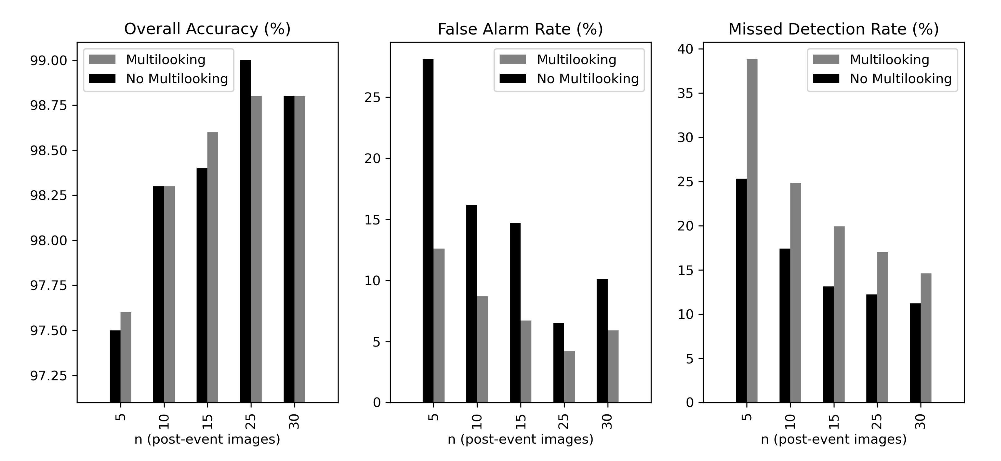
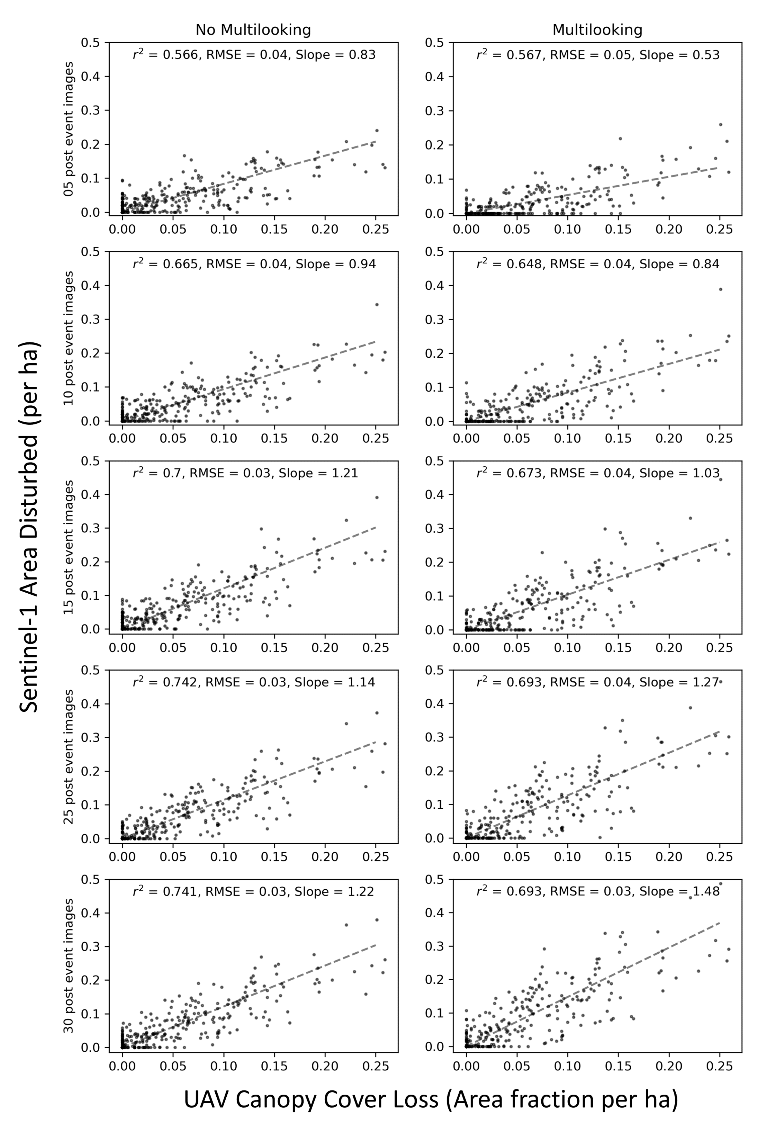
3.1. Canopy Gaps Most Accurately Quantified Using 25 Post-Disturbance Images

Areas of S-1 shadow corresponded closely to canopy gaps detected by LiDAR, and the best validation results were obtained using 25 post-event images and by skipping the multilooking step. As shown in Figure 3, shadows were spatially offset relative to canopy gaps by up to 20 m in random directions, and multiple canopy gaps sometimes merged into a single shadow and vice versa. The spatial patterns, however, indicated that overlap between a shadow and a canopy gap was a good indicator that they corresponded to the same physical event.
For n = 25 and with no multilooking, our S-1 change detection algorithm had an accuracy of 99.0% and a false alarm rate—taking into account all canopy gaps down to 0.01 ha—of 6.5%. As shown in Figure 4, this was slightly higher than the false alarm rate of 4.2% obtained when using multilooking. However, not multilooking led to a more significant decrease in the missed detection rate (12.2% compared to 25%). The missed detection rate was slightly improved by increasing the number of post-event images to 30, but this was counteracted by an increase in false alarms. Multilooking always resulted in a lower false alarm rate but more missed detections (Figure 4) for a given n. With respect to disturbances larger than 0.1 ha, n = 10 was sufficient to ensure all 37 canopy gaps were detected as long as multilooking was applied. No combination of parameters caused a false alarm greater than 0.1 ha in size.

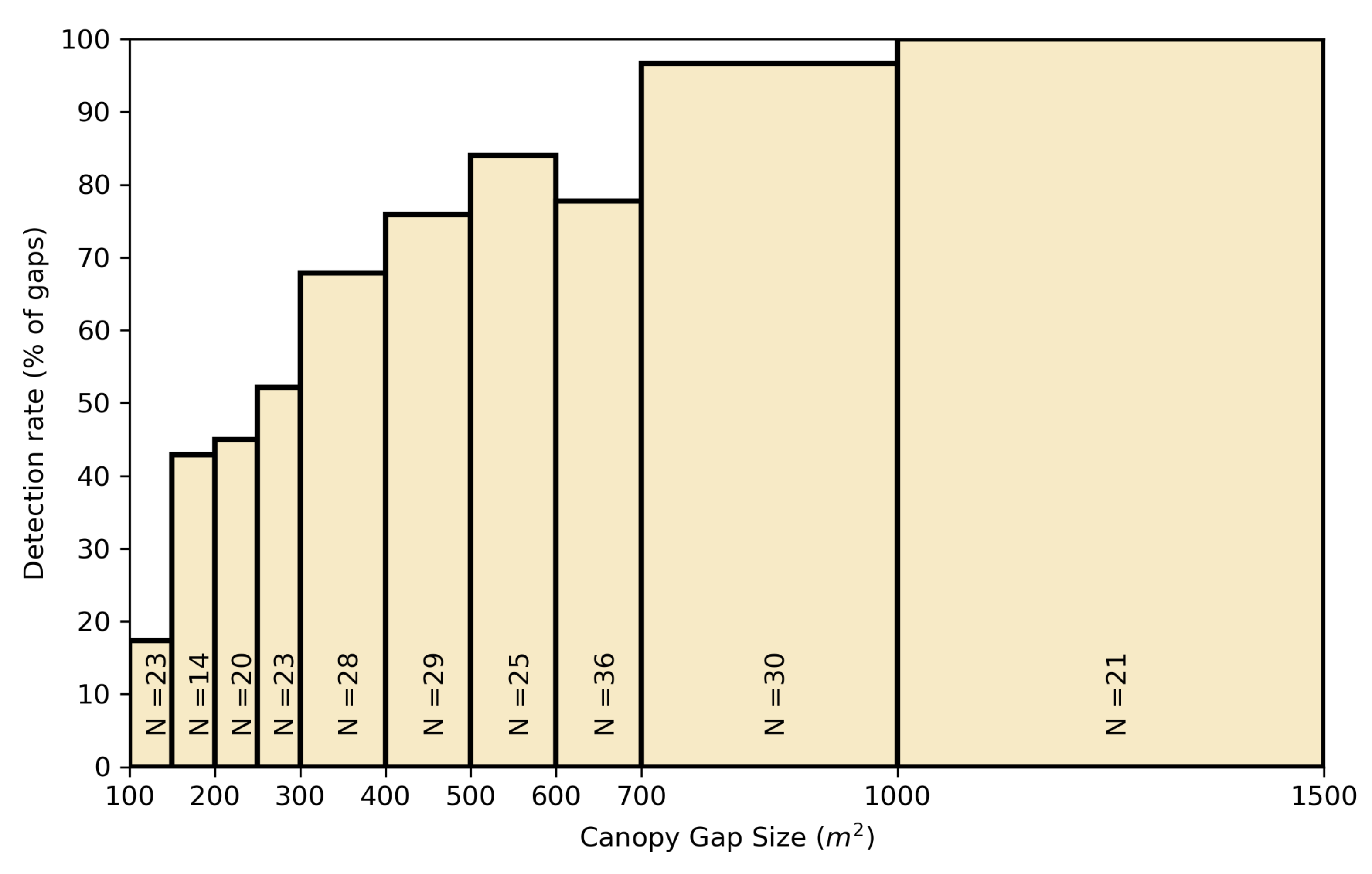
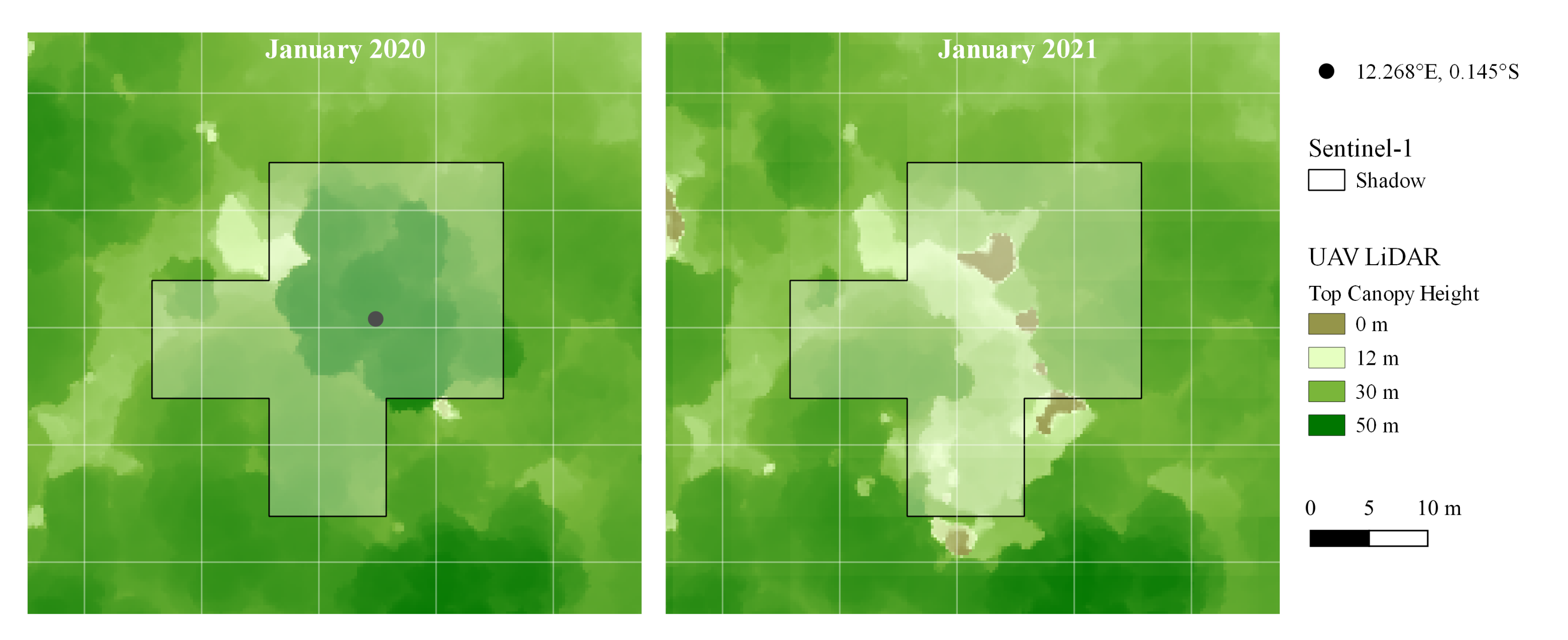
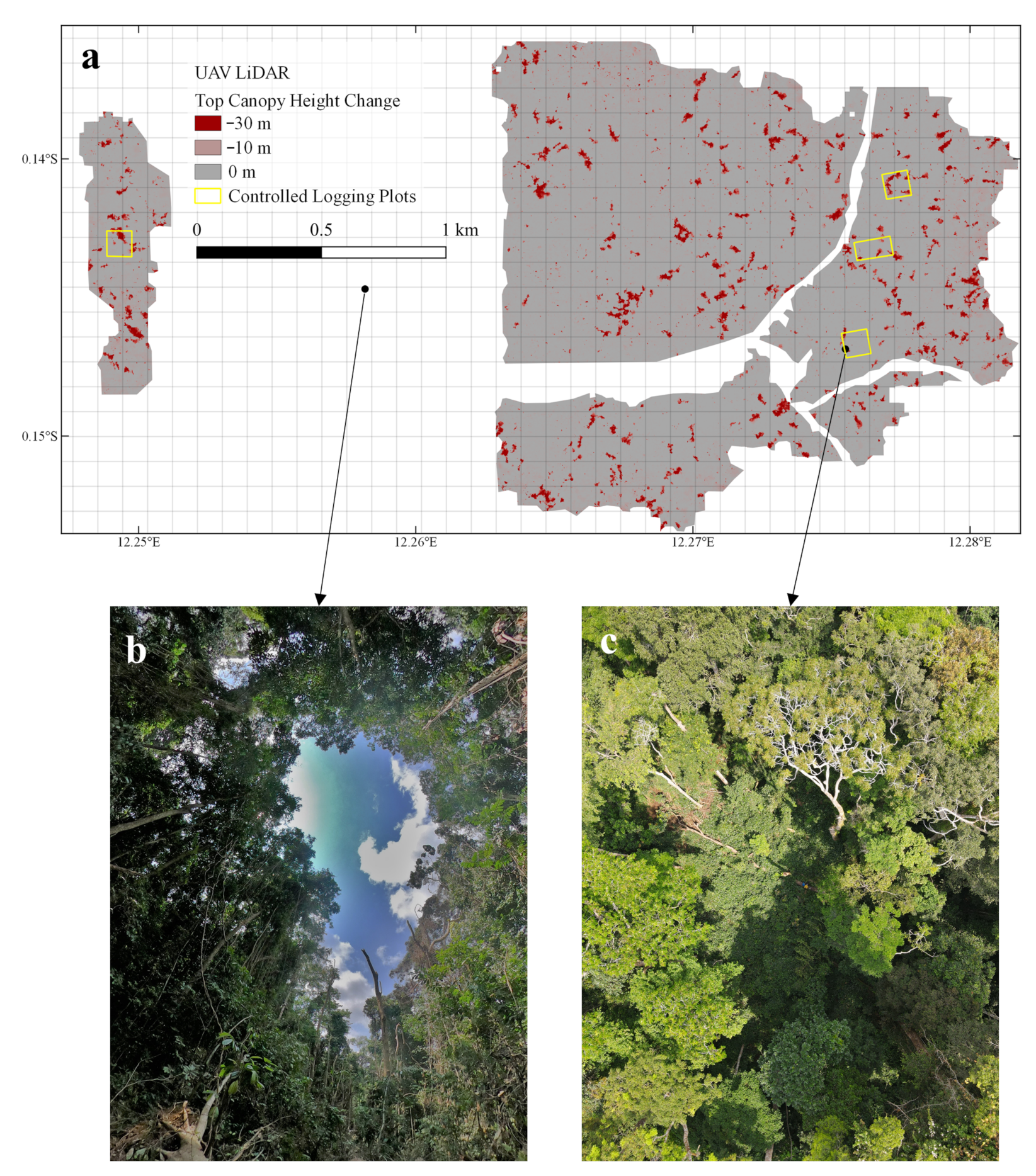
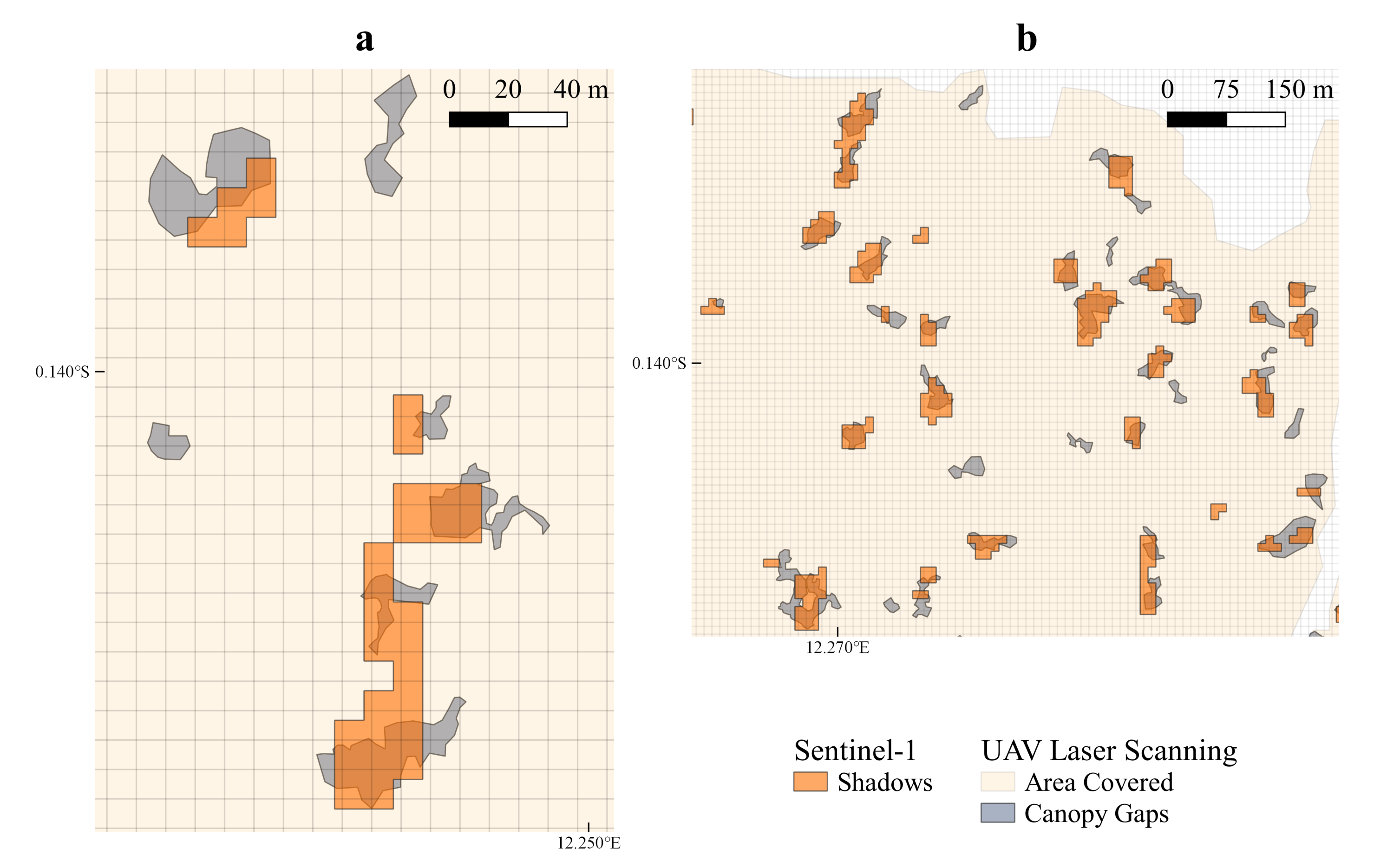
3.2. Canopy Gaps Detected down the Scale of Individual Trees

Our S-1 shadow detection algorithm picked up the majority of canopy disturbance caused by gaps smaller than 0.05 ha (when using n = 25 and no multilooking). We found 65% of disturbed area in gaps between 0.01 and 0.05 ha was correctly identified, and 69% of S-1 pixel area in shadows of this size corresponded to true canopy gaps. Top canopy height obtained using the UAV LiDAR confirmed that many of these smaller gaps were the result of single tree disturbances. For gaps between 0.05 and 0.1 ha, 90% of area was correctly identified and 95% of S-1 shadow area corresponded to true detections, while no errors were made at all for gaps larger than 0.1 ha (see Table A1 for all size-stratified false alarm and missed detection rates for different algorithm parameters, and Figure A1 for an example of a single tree crown removal).
The detection rate of individual disturbances is shown as a function of gap size in Figure 5. Most gaps smaller than 175 m2 (0.0175 ha) were not detected—as might be expected given that we filtered out isolated 10 m × 10 m pixels—but there appears to be a sharp increase in detection rate around 200 m2 (0.02 ha), and a steady increase with a gap size beyond that point. The number of detections reaches 90% at around 500 m2 (0.05 ha) and 100% at 1000 m2 (0.1 ha).

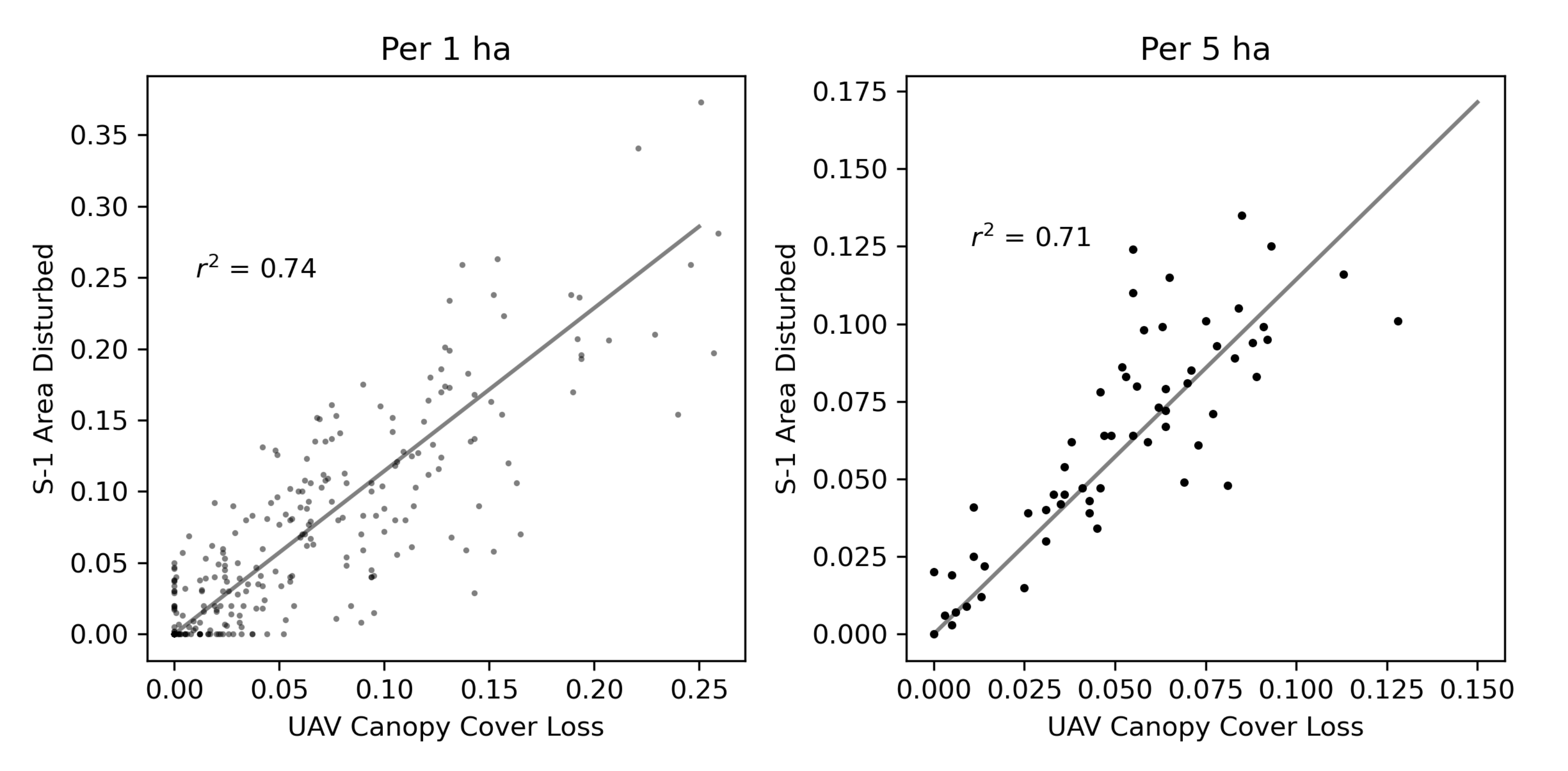
3.3. Canopy Cover Loss Quantified by Linear Relationship to S-1

A linear relationship was observed between the area of UAV canopy cover loss and the area of S-1 shadows detected when considering larger pixels. Holding n at 25 and not multilooking gave the highest correlation: at a scale of 1 ha, r 2 was 0.74, which fell slightly to 0.70 if n was reduced to 15 and to 0.69 if multilooking was used. In general, multilooking led to slightly weaker relationships, but the difference was less pronounced for lower n. For example, at n = 10 , r 2 was 0.65 with multilooking and 0.67 without it. The weakest relationship had r 2 = 0.57 , and was obtained when only five post-event images were used.
As shown in Figure 6, the linear relationship between canopy cover loss and S-1 shadows held when aggregating to a scale of 5 ha, with an r 2 of 0.71 (see Figure A2 for scatter plots of all tested algorithm parameters). The root mean square error (RMSE) of the fraction of canopy disturbed at 1 ha was 0.03, and reduced to 0.01 at 5 ha. Our data show no obvious deviation from a linear relationship up to canopy cover loss levels of around 25% per ha or 10% per five ha; we cannot test the relationship beyond this point as we have no UAV training data where greater proportions of 1 or 5 ha boxes were disturbed.

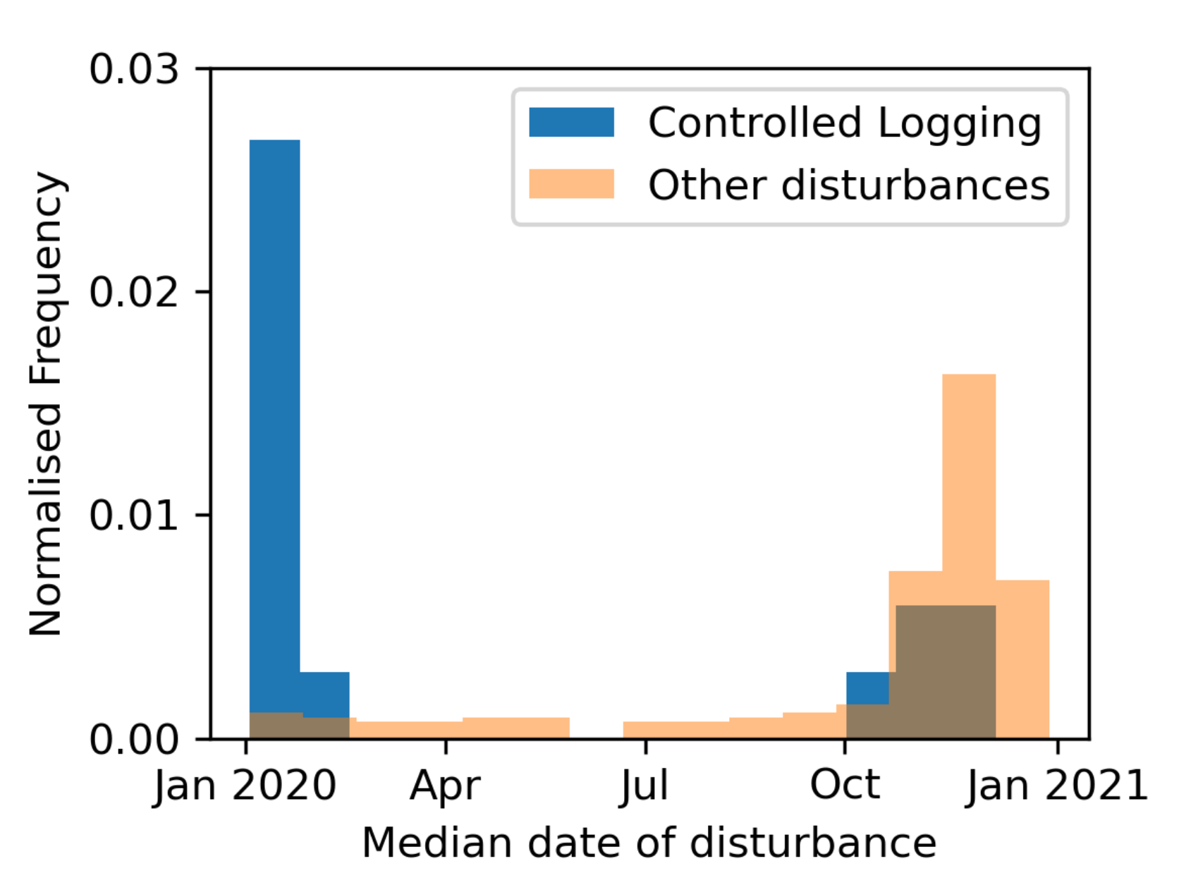
3.4. Temporal Match between S-1 Shadows and Logging Experiment

The estimated timing of S-1 shadows in our study area matched the time of known forest disturbances. Shadows overlapping canopy gaps created between 24 January and 28 January 2020 as part of our controlled logging experiment appeared predominantly at the start of the year, as shown in Figure 7. For other shadows in the area, most identified as appearing after October. This matches communication from Rougier Gabon that recorded this parcel of the concession to have been logged in November and December 2020.
Figure 7 shows that some of the disturbances in the experimental logging plots were detected by Sentinel-1 around the same time as the wider area was logged. This is likely to be a true detection as the felled logs in these plots were removed and more trees around the plots were logged at this time, causing further disturbance to the canopy. Outside of the main disturbance period towards the end of the year, there is a low level of shadow emergence throughout the year, which is to be expected given both the natural dynamics of a tropical rainforest and the non-zero level of false alarms generated by our algorithm (Figure 4).

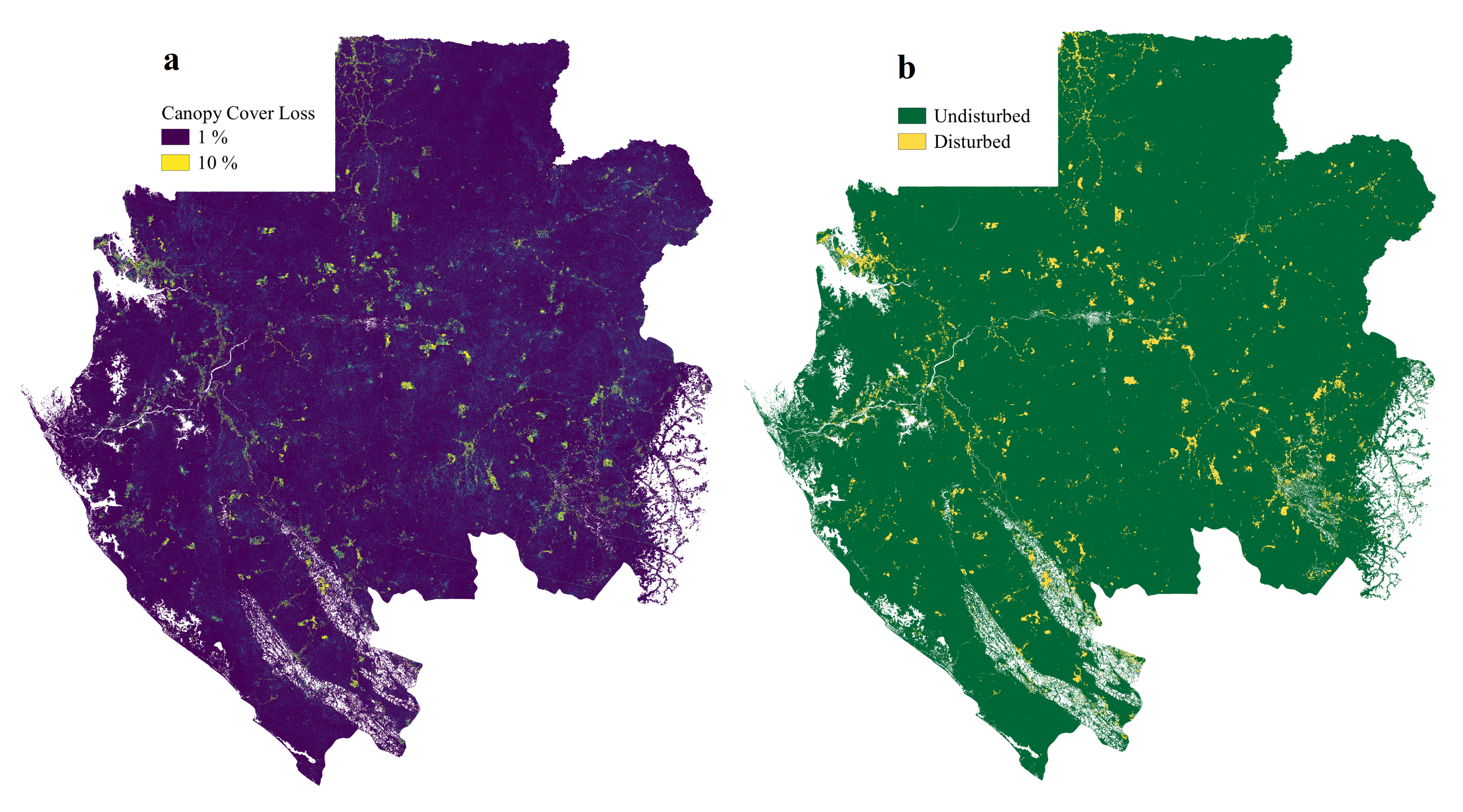
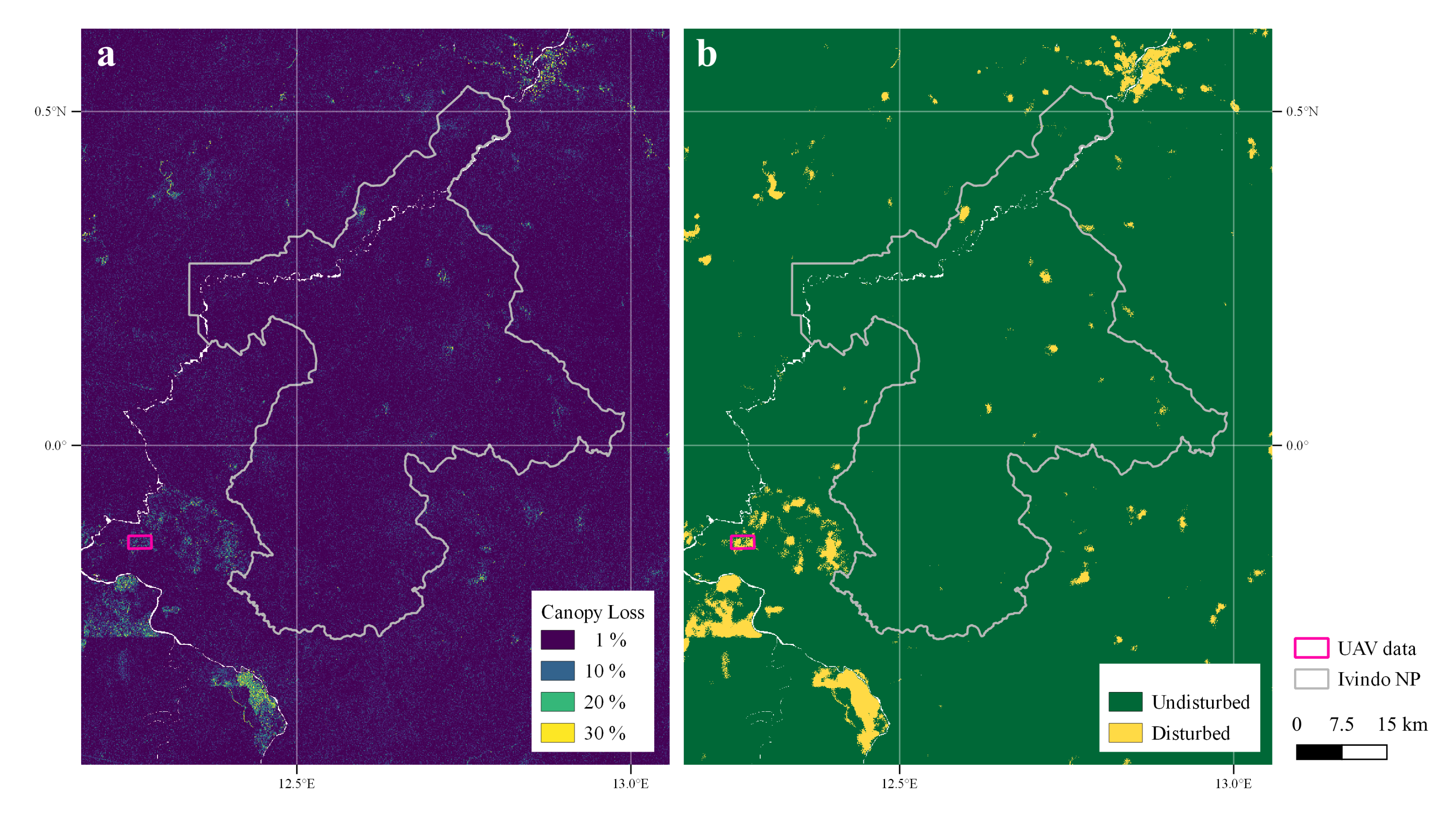
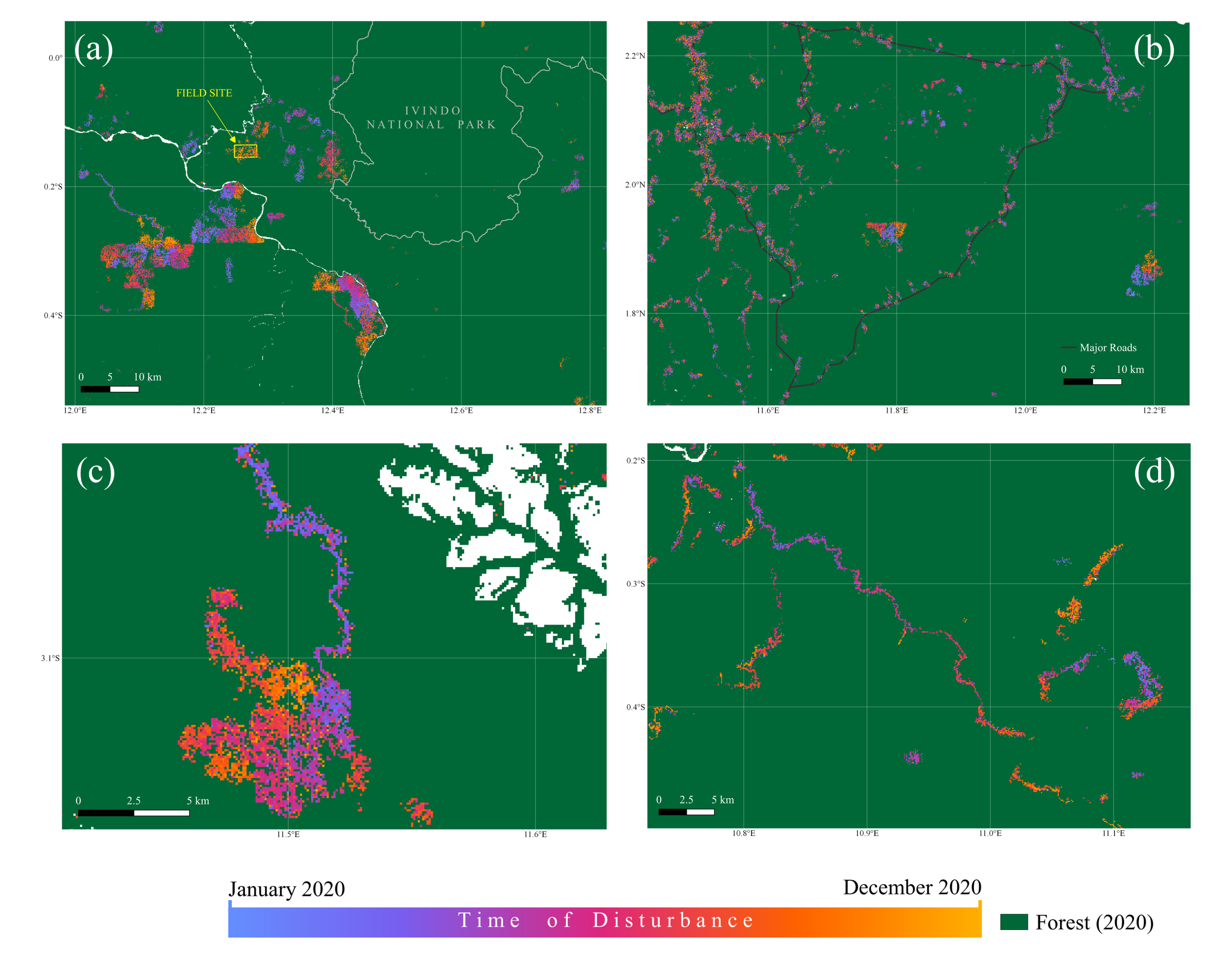
3.5. Degradation Maps of Gabon for the Year 2020

Application of our S-1 algorithm across Gabon produced a plausible map of canopy cover loss showing the location and extent of degradation in 2020, as well as enabling a quantification of human and natural degradation levels. Our RF classification of the map into disturbed and undisturbed regions performed extremely well, miss-classifying only 2 ha of undisturbed forest as disturbed out of a testing dataset of 2705 ha, corresponding to an overall accuracy of 99.9%. An overview of the canopy loss map and disturbance map is given in Figure 8, which shows the highly heterogeneous nature of the degradation patterns. Both maps can be viewed online at https://harrycarstairs.users.earthengine.app/view/fodex-gabon-2020, accessed on 18 April 2022.
Across Gabon, we estimate that around 3% of forested areas were disturbed in the year 2020 (including 1-ha cells degraded directly and those in close to proximity to high levels of degradation). Within national parks, anthropogenic disturbance was much lower at 0.4%. The gross area of canopy cover lost according to our map was 0.31 Mha, representing 1.3% of the country’s 24.2 Mha of forested land. It should be noted that this is not an estimate of net canopy cover change, as our algorithm makes no estimate of canopy cover gains.
Our classification allows us to compare levels of canopy cover loss in what we classify as disturbed and undisturbed forest. We find these differ by an order of magnitude, with disturbed areas losing 9.6% of their canopy cover compared to 1% in undisturbed areas.
A larger scale example of our canopy cover loss and disturbance maps is given in Figure 9 for a region including Ivindo National Park and our field site. The losses around the field site are clearly visible, as are other logging parcels to the North and East that do not encroach beyond the boundary of the national park. South of the Ogooue river, another logging concession is visible by its clear boundaries (e.g., unnaturally straight lines) and appears to more heavily logged than the field site. Two other patterns are visible: in the national park, there are only smaller and less intense clusters of degradation; and, in the northeast corner, degradation fans out around the edges of a town (Makokou) and the roads leading into it.
Four examples of temporal degradation patterns are shown in Figure 10. In regions of remote forest, the timing of disturbance appears to be systematic across large, contiguous blocks. Within these blocks, there are distinct boundaries between patches disturbed at different times of the year, patches that spread uniformly in time, and relatively few anomalies to these patterns. Some linear disturbances (Figure 10d) show a remarkably strong relationship between distance along the feature and the time of disturbance. Around towns and roads, however, temporal patterns are less ordered (Figure 10b). Here, we observe much less of a relationship between the timing of degradation events in adjacent pixels, and very few large scale trends.

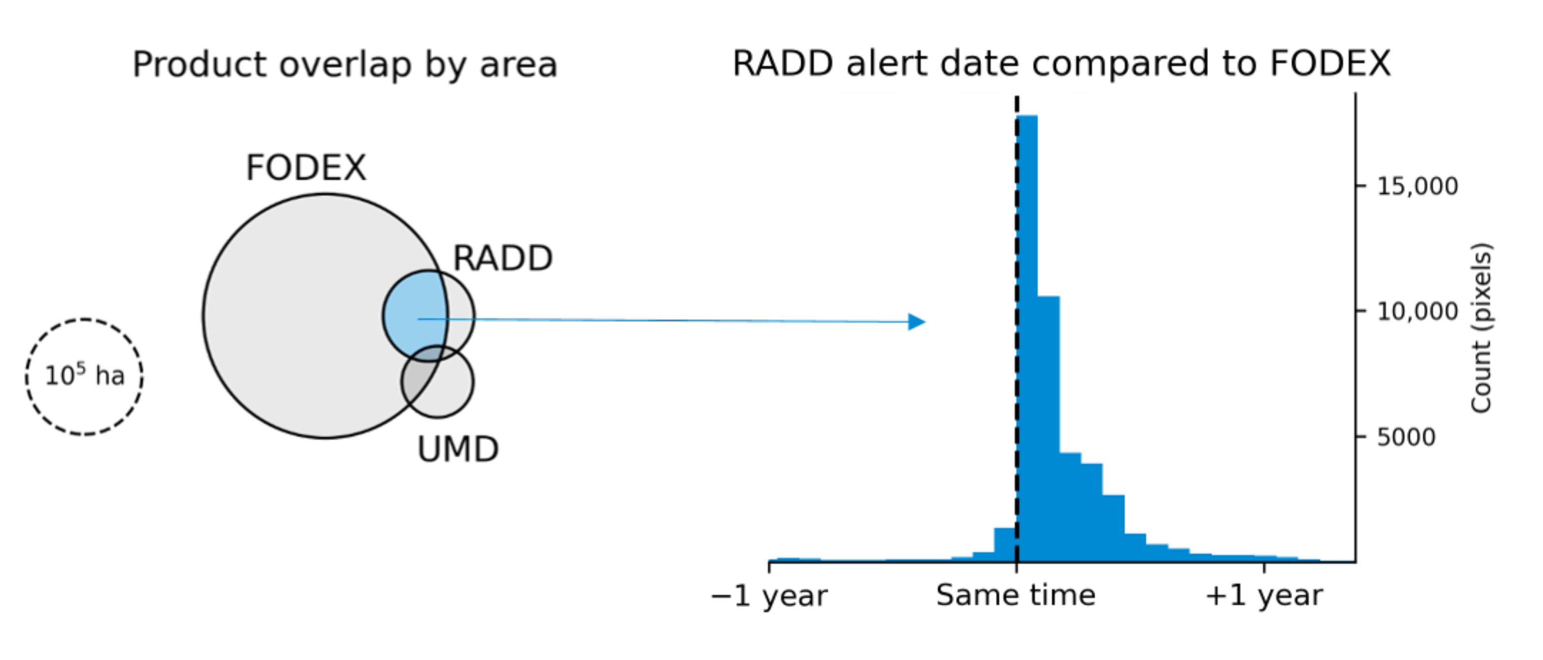
3.6. Comparison to RADD and UMD Products

Here, we compare our Sentinel-1 algorithm to two published products: the RADD disturbance alerts [48], based on S-1; and the UMD forest loss maps [41], based on Landsat. The majority of disturbances at our study site were not detected by RADD. Out of 261 canopy gaps identified in the UAV data (37 of which were larger than the minimum mapping unit of 0.1 ha for RADD), only six were intersected by alert pixels assigned to dates between the two UAV acquisitions. In total, these RADD alert pixels covered an area of 0.65 ha, less than 5% of the 16.09 ha of canopy loss. If alerts assigned to dates up to the end of 2021 are included, eight gaps are detected by alert pixels covering an area of 2.23 ha. Excluding gaps smaller than 0.1 ha, this still corresponds to a missed detection rate of 68.1%. The Landsat-based UMD product [41] did not detect any forest loss in the study area in the year 2020.
Over the whole of Gabon, the gross area of canopy cover loss we estimate is significantly higher than the areas of disturbance detected by the UMD and RADD alert systems, as shown in Table 2. This is despite the fact that both UMD and RADD pixels can include partial canopy losses, meaning this is an absolute upper bound to the area of canopy loss they detect.
Most RADD alerts for the year 2020 were located in areas also flagged by our algorithm as having high levels of degradation, while there was less overlap with UMD forest loss. The majority of canopy loss we detect is spatially separate from either RADD or UMD alerts. We illustrate this in Figure 11, which shows the overlap between 1-ha cells containing disturbances greater than 10% for each of the three products.
We found a temporal discrepancy between our estimated disturbance dates and those given by RADD. In general, we predicted an earlier disturbance date. Figure 11 shows that, in 1-ha cells across Gabon (where the products overlap), the median date of disturbance is sometimes as much as six months later.

4. Discussion

By using UAV LiDAR to create a highly accurate reference dataset of selective logging, we have demonstrated the potential of S-1 SAR timeseries to map degradation down to fine scale canopy disturbances well below 0.1 ha. Our algorithm detected the emergence of new SAR shadows using a change ratio, and we found a strong linear relationship between the area of shadow pixels and canopy cover loss, making it possible to quantify the full extent and severity of forest degradation. This approach to degradation mapping was easily scalable, as we demonstrated by creating an experimental product covering the entire forested area of Gabon (24.2 Mha). Furthermore, spatial and temporal patterns in this product can be used to create a convincing separation of anthropogenic disturbances from natural forest dynamics.

4.1. Trade Off between Timeliness and Accuracy

The most accurate S-1 algorithm we tested relied on having a time-series of 50 images to estimate shadow emergence in single S-1 GRD pixels without any further spatial averaging (Figure 4). Although maps using this method could be updated every 12 days as new S-1 imagery becomes available, the nature of the algorithm would necessitate a 10 month delay between a degradation event and its final quantification. Attempting to quantify degradation sooner than this led to higher false alarm rates and missed detection rates, particularly with respect to smaller disturbances. By increasing the number of post-degradation images used to detect a drop in backscatter, it became possible to smooth out the effects of speckle within an individual 10 m pixel, instead of relying on multilooking which achieves this at the cost of spatial resolution. Multilooking still improved accuracy for shorter timeseries, especially for larger canopy gaps: only when 25 post-event images were available did it appear beneficial to analyse shadows at the individual pixel level. Overall, it appears there is a trade-off situation between timeliness and accuracy, and that sacrificing NRT capability makes it possible to fully utilise Sentinel-1’s spatial resolution and detect disturbances smaller than 0.05 ha.
If we consider only disturbances greater than 0.1 ha, however, these were detected perfectly (no false alarms or missed detections) after 4 months of S-1 imagery using our algorithm. This observation is in line with the results of previous studies that found high accuracy for S-1 forest alert products when applying a minimum mapping unit of 0.1 ha [40,45,46,49]. We suggest, therefore, that both approaches are important: NRT systems should be used as a means of rapidly identifying the location of large disturbances; and these should be backed up in due course by accurately quantified maps of canopy loss when enough S-1 imagery is available to discern the smallest possible changes. As there was still a strong relationship between canopy cover loss and S-1 shadows using 10 post-event images (r = 0.82 for 1 ha cells), it would also be reasonable to produce provisional quantified degradation maps after four months where there is a need for more rapid assessments.
Our long time-series approach also appeared to result in better temporal accuracy than current NRT systems. For example, we compared our field data to the RADD alerts, and found that many disturbances occurring between January 2021 and January 2022 were assigned to dates later in 2022 (sometimes up to 200 days after the second UAV flight). This contrasts to our S-1 algorithm which differentiated extremely well between two waves of disturbance in 2021 (Figure 7) and appears to have an accuracy of around a month. Over the whole of Gabon, the RADD alert system generally estimated later disturbance dates than our algorithm, perhaps because it relies on a single pixel value to trigger the alert [48], which may mask smaller but persistent changes in backscatter. While a full quantification of temporal accuracy was not possible as precise reference data for disturbance dates was not available, it appears that NRT products may not always provide the best indication of when a disturbance occurred.
For our study area, increasing the number of post logging images to 30 led to an increase in false alarms. This may be due to gradual changes from forest growth and regrowth causing a significant enough change over this period to SAR backscatter that the shadow threshold is breached. This should be investigated further in faster growing forests (for example in parts of the Amazon) where this effect may be stronger and a shorter observation period would be available, or additional processing would be required to filter out gradual changes in backscatter.
It should be noted that the delay of our product is due to the number of images required, so it is proportional to the revisit period of the satellite. If, for example, a C-band satellite with a 6-day revisit time was available, this could reduce the time between degradation and quantification to five months.

4.2. Detection of Fine Scale Disturbances

We have shown that the removal of a single canopy tree in a tropical forest can lead to a detectable signal in S-1 backscatter. UAV LiDAR highlighted the importance of detecting such events, as we found that, in an area of selectively logged forest, more than half of canopy gaps were smaller than 0.05 ha and 62% of disturbed area was caused by gaps below 0.1 ha: a degradation mapping tool that excluded these disturbances could severely underestimate degradation, and miss whole regions of degradation typified by multiple small clearances. For comparison, many previous attempts to detect selective logging from satellite data have worked at the 0.09 ha scale of Landsat pixels [64,65,66,67]. Although there is evidence that disturbances as small as 25% of a Landsat pixel can be detected [68], this relies on a cloud free image being available from the short period during which the disturbed area shows bare ground and therefore a strong optical difference to the canopy, which is likely to lead to high missed detection rates in cloudy tropical regions. Previous studies using S-1 have typically applied a minimum mapping unit of 0.1 ha or larger [40,45,46,48] in order to prioritise accuracy of individual disturbances.
Our UAV data allowed us to study canopy gaps that would have been impossible to identify using any known passive optical satellite: no cloud free optical images (openly available or commercial) were found within six months of our selective logging experiment, by which time the majority of disturbance would have turned green again [43]. Multi-temporal UAV LiDAR is therefore a crucial stepping stone between field inventories and satellite remote sensing of tropical forests. While the fieldwork comes with challenges (e.g., cost, locating suitable take-off/landing zones in an area being logged, and maintaining relatively newly developed technology in a new environment), we have shown that it is feasible and effective, and provides rich data. We recommend an effort to continue collecting this kind of data to aid the development of satellite degradation products.
We have shown that, when considering smaller disturbances, it is possible to process S-1 data entirely using pixel based operations, thereby reducing computing cost compared to object based methods. We found the minimum detectable size to be around 0.02 ha (Figure 5), which is two S-1 GRD pixels. Including shadows consisting of single S-1 GRD pixels led to excessive false alarms, which should be expected given the fact that the pixel size of 10 m is less than the azimuth resolution of the raw radar images: real SAR shadows are therefore likely to affect the backscatter in multiple pixels even if they are smaller than 10 m.
Our threshold ratio was small (0.64 dB reduction) compared to those used in previous studies (typically at least 3 dB reduction [40,46]), and this may have allowed the detection of sub-resolution sized shadows (noting that the physical size of a SAR shadow is a different quantity to both the canopy gap area and the area of pixels classed as containing a shadow). We can imagine a situation where a small canopy gap leaves a SAR shadow that is strong, say −5 dB compared to the original backscatter value, but extends only a few metres in the range direction of a SAR sensor. The resulting pixel will be a mixture of the shadow and other surrounding scattering components, so will see a drop of less than 5 dB, but if the shadow is real, it will be a consistent decrease that is detectable using our long time series approach.
Considering that, even for the most accurate parameters, the false alarm and missed detection rates were 6.5% and 12.2%, respectively, it is clear that the result of our algorithm should not be used as firm evidence of a single canopy gap smaller than 0.1 ha. Additionally, as Sentinel-1 has an azimuth resolution of 20 m and GRD georeferencing adds error in hilly regions, we estimate that our shadow mapping has a spatial uncertainty of up to 20 m and should therefore not be used for precision mapping of any particular disturbance. The strength of our approach lies in the fact that the errors appear to be randomly distributed and therefore become small when scaling up to larger areas: with these errors known, good estimates of the degradation occurring in a district, logging concession, national park or region can be estimated, as well as their temporal evolution through a year.
Some canopy gaps were missed: sometimes this occurred following the removal of crowns that were already in the shadow of a taller tree before they were removed. Other factors which are likely to affect the sensitivity of S-1 to canopy gaps include the orientation (relative to radar range direction), shape, and depth of gaps, which in turn are driven by the heterogeneity and average height of a forest canopy as well as average crown size. An in-depth analysis of these factors was not appropriate given the limitations of a single field site, but future work should investigate these factors using comparable canopy gap data from another tropical forest with different physical characteristics.
Some parts of the tropics are generally covered by both S-1 satellites with different pass directions. In such areas, the different viewing angles would pick up different different shadows: this may be useful for delineating larger patches of forest loss ([40]) and potentially reduce the missed detection rate; in the case of small gaps, it would possibly lead to an overestimation if shadows from both passes were added together. Instead, it may be better to use one pass direction or another depending on which gives a preferable viewing angle, thereby avoiding slopes facing the sensors where the signal quality is poorer ([53]).

4.3. Relationship between S-1 Shadows and Canopy Cover Loss

Our shadow detection algorithm is strongly correlated to UAV canopy cover loss at a 1 ha scale ( r 2 = 0.74 ) when 25 post-event images are used. Both our accuracy and correlation assessments can be considered conservative estimates due to the fact that some errors in our S-1 product will be temporal rather than spatial. For example, some disturbances which occurred before the first or after the second UAV flight may be included, while disturbances just after the first or just before the second UAV flight may be excluded, which due to the fact our algorithm prioritises spatial resolution over temporal resolution. This is likely, given that logging activities were occurring at the field site around the times of both UAV flights. These errors should not be important for annual statistics, where they would only lead to a small mixing of disturbance attribution between successive years.
We may underestimate the area disturbed in larger canopy gaps where bare ground is visible to the sensor—here soil moisture and regrowth could cause the backscatter to quickly return to previous value. In this case, an object based algorithm may be more appropriate, with the potential to use multiple pass directions or the increase in backscatter on the far range edge of a clearing to delineate its edges [40]. On the other hand, our threshold parameter may already be small enough to differentiate directly between canopy and areas of regrowth—field data with larger cleared patches will be required to test this in future studies.
It may be that the type of degradation has an influence on the relationship between S-1 shadow and canopy loss, as the typical form of canopy disturbance may be different depending on the activity (for example small scale mining, agriculture or road building). This should be tested using reference data from different forms of degradation. The more dynamic, faster growing forests of Amazonia may require different algorithm parameters, and may have a higher uncertainty as backscatter values will be less stable over long periods of time. Seasonal effects and weather events should be well controlled for by the use of 25 images spanning 10 months either side of a disturbance event. This should, however, be tested in areas with strong seasonality such as flooded forests and peat forests where soil moisture may cause significant backscatter variations. Our relationship was built entirely on canopy gaps, but forest degradation and loss also occur at forest edges. The response of S-1 in this scenario would be more dependent on viewing angle, so a more complicated approach and multiple pass directions may be required.
Our algorithm predicts gross canopy cover loss with a root mean square error (RMSE) of 0.03 at a 1 ha scale. It therefore gives a clear indication of human disturbance, which leads to losses of 10–20%, but would not be suitable for identifying subtle graduations at the 1 ha scale between very low levels of degradation. Aggregating to 5-ha, however, we find the relationship improves for areas with low levels (<5%) of degradation and the RMSE lowers to 0.01. This shows that our approach is promising for accurate quantification of degradation levels at larger scales. We estimate the area of gross canopy cover loss in Gabon for 2020 to be 0.31 Mha. The uncertainty in this figure from propagating the 3% errors at 1 ha scale would be just ± 150 ha. However, this assumes that the errors are randomly distributed over a variety of conditions not tested in our field data, as discussed above, so we expect that the true uncertainty is higher than this.

4.4. Potential for Wide Area Quantification of Degradation

Figure 8 indicates highly clustered disturbances across Gabon, as would be expected given the fact that majority of the country’s forest is either national park or allocated as a logging concession. Our map shows very clear signs of selective logging activities including large parcels of remote, disturbed forest with clear boundaries that are disturbed methodically through the year. New logging roads are also highlighted, many of which can be linked directly to the patches of selective logging. In addition, our map shows some other patterns of disturbance around more densely populated areas, which we suggest are the result of small scale agricultural expansion. We chose to limit our initial map to Gabon as it has a low population density, a large area of protected forest, and the vast majority of forest disturbance is due to selective logging across large concession areas. We recommend that, to apply our method to countries with different drivers and patterns of degradation or different forest structures, additional bi-temporal laser-scanning data would be necessary for validation.
Overall, our results are in agreement with Gabon having much higher levels of forest degradation than deforestation. The area we classify as having been locally disturbed in 2020 is about 35 times that which was deforested according to the UMD product. Our figure of 1% gross annual canopy cover loss is consistent with plot data [69] that estimates natural tree mortality rates in this area to be around 1%. Although the distribution of tree canopy sizes is skewed towards smaller canopies, this is counteracted by an increasingly mortality rate with size, suggesting that a figure of 1% canopy cover loss is reasonable.
By comparison, the total area of RADD alerts in Gabon for 2020 was below 0.02 Mha. This value is much lower than our estimated canopy loss because the RADD system prioritises low false detections rather than overall accuracy in quantifying degradation, and because it omits any disturbances below 0.1 ha (which we have shown are important drivers of degradation in areas of selective logging). Over three quarters (77%) of RADD alerts occurred within areas we classified as disturbed, and inspection of the remaining RADD alerts outside of disturbed areas suggests the majority of these are also human disturbances, and were classed as undisturbed in our map due mainly to a difference in temporal allocation. This highlights the strength of the RADD alert system in its ability to pick out areas likely to be affected by human activities, while also showing the need for more sensitive algorithms if we are to fully quantify both anthropogenic and natural forest degradation.
Regularly updated maps of forest cover will be important for degradation mapping. We used a map for the year 2020, and others are available based on a range of satellite products. To avoid double counting, degradation products must be carefully explicit about what is included and excluded. For example, we found some overlap between our product and pixels classed as forest loss in the Landsat-based UMD product (Figure 11). A minimum time between multiple disturbances of the same pixel will also need to be determined for long-term degradation mapping, which may be a function of forest and disturbance type.
Our map of Gabon required some manual calibration to ensure consistency between scenes. Going forward, an automated approach towards image quality assurance, scene calibration and mosaicking should be developed as a step towards an operational product.
Maps of anthropogenic disturbance should be improved by using industrial or government data for example on forest concessions and mining activity, instead of relying on interpretation of degradation patterns. Some natural disturbances may be included in our map of disturbed regions, as large areas of windfall of landslides would present a similarly intense, temporally concentrated pattern of damage to anthropogenic disturbances. Combining canopy loss maps with other mapping techniques will help to differentiate these kinds of degradations.

5. Conclusions

We have presented an algorithm to estimate annual gross canopy cover loss due to small scale disturbances in tropical forest. The algorithm relies on the power of a long time series to detect small but persistent decreases in Sentinel-1 backscatter caused by the radar shadows that emerge from new canopy gaps as small as 0.02 ha. A linear relationship was found between the area of Sentinel-1 shadow and canopy loss for intensities between 0 and 25% loss per hectare, but further work is required to verify if this relationship continues beyond 25%, and if it is affected by factors such as forest height, type, terrain or seasonality. Given these issues that are addressed, our algorithm could be used to create spatially contiguous, quantified maps of forest degradation, something we have demonstrated for the country of Gabon. Such maps would be an important step towards measuring AGB change across the tropics, monitoring logging activities, and verifying decreases in degradation for carbon payment schemes, as well as providing insights into natural forest dynamics.

Author Contributions

Conceptualization, H.C., E.T.A.M. and M.D.; methodology, H.C.; validation, H.C.; formal analysis, H.C.; resources, E.C. and M.O.E.; data curation, I.M., C.A. and A.M.D.; writing—original draft preparation, H.C.; writing—review and editing, E.T.A.M., I.M., C.A. and M.D.; visualization, H.C.; supervision, E.T.A.M. and M.D.; project administration, E.T.A.M.; funding acquisition, E.T.A.M. All authors have read and agreed to the published version of the manuscript.

Funding

This research was funded by the Tropical Forest Degradation Experiment (FODEX)—European Research Council Grant No. 757526.

Data Availability Statement

The code and data required to reproduce our results are available at https://code.earthengine.google.com/?accept_repo=users/harrycarstairs/FODEX_S1_Gabon_2020, accessed on 18 April 2022. Our results for canopy cover loss in Gabon 2020 can be viewed on an interactive map at https://harrycarstairs.users.earthengine.app/view/fodex-gabon-2020, accessed on 18 April 2022.

Acknowledgments

We would like to thank the staff of Rougier Gabon, including Evanillho Téodoro Muaño Bondjale and Aimé Manfoumbi, for hosting us in Ivindo and cooperating to make our fieldwork there possible. While in Gabon, we also received invaluable support from Alfred Ngomanda, Lee White, the Agence Nationale des Parcs Nationaux (ANPN), the Ministry of Water and Forests, the Sea and the Environment, the Research Institute for Tropical Ecology (IRET), and our field assistants, especially Joseph Amelim Boukandja, from the Ivindo community. We thank the Natural Environment Research Council (NERC) Geophysical Equipment Facility for the loan of GNSS receivers.

Conflicts of Interest

The authors declare no conflict of interest. The funders had no role in the design of the study; in the collection, analyses, or interpretation of data; in the writing of the manuscript, or in the decision to publish the results.

Appendix A

Table A1. Area based accuracy of Sentinel-1 shadow at detecting canopy gaps in 310 ha of forest, 5.2% of which was classified as disturbed from multi-temporal UAV LiDAR data. The canopy gaps are split into small (0.01 to 0.05 ha, N = 134), medium (0.05 to 0.1 ha, N = 90), and large (0.1 to 0.5 ha, N = 37). Results are shown according to how many post-event images were made available (n). A further distinction is made between results with or without a 3 × 3 multi-looking filter, and the best results are highlighted in bold.
nMulti-LookAccuracyFalse Alarm Rate (% Area)Missed Detection Rate (% Area)
(Images) (%)TotalSmallMediumLargeTotalSmallMediumLarge
5x97.528.152.39.70.025.354.926.75.1
🗸97.612.633.810.20.038.873.048.47.4
10x98.316.245.46.20.017.445.112.25.1
🗸98.38.730.814.60.024.856.829.30.0
15x98.414.753.16.10.013.137.29.11.8
🗸98.66.737.69.70.019.953.118.60.0
25x99.06.530.55.50.012.235.39.80.0
🗸98.84.230.310.60.017.048.014.30.0
30x98.810.144.45.90.011.231.79.40.0
🗸98.85.938.518.00.014.640.013.00.0
Figure A1. UAV LiDAR Top Canopy Height in January 2020 and January 2021 showing the removal of a canopy tree, overlaid with the area of shadow detected by our S-1 algorithm.
Remotesensing 14 04233 g0a1
Figure A2. Area of Sentinel-1 Shadow per 1 ha cell vs. area of UAV LiDAR detected canopy gap. Results are separated for various values of n, the number of post-event images used in to estimate S-1 shadows, and according to whether 3 × 3 spatial multilooking was applied. In each case, the correlation coefficient r, root mean square error (RMSE) and ratio of S-1 shadows to UAV canopy gap area (slope) is indicated.
Remotesensing 14 04233 g0a2

References

  1. Gatti, L.V.; Basso, L.S.; Miller, J.B.; Gloor, M.; Domingues, L.G.; Cassol, H.L.; Tejada, G.; Aragão, L.E.; Nobre, C.; Peters, W.; et al. Amazonia as a carbon source linked to deforestation and climate change. Nature 2021, 595, 388–393. [Google Scholar] [CrossRef] [PubMed]
  2. Hubau, W.; Lewis, S.L.; Phillips, O.L.; Affum-Baffoe, K.; Beeckman, H.; Cuní-Sanchez, A.; Daniels, A.K.; Ewango, C.E.; Fauset, S.; Mukinzi, J.M.; et al. Asynchronous carbon sink saturation in African and Amazonian tropical forests. Nature 2020, 579, 80–87. [Google Scholar] [CrossRef] [PubMed]
  3. Mitchard, E.T. The tropical forest carbon cycle and climate change. Nature 2018, 559, 527–534. [Google Scholar] [CrossRef] [PubMed]
  4. Baccini, A.; Walker, W.; Carvalho, L.; Farina, M.; Sulla-Menashe, D.; Houghton, R. Tropical forests are a net carbon source based on aboveground measurements of gain and loss. Science 2017, 358, 230–234. [Google Scholar] [CrossRef]
  5. Allen, C.D.; Macalady, A.K.; Chenchouni, H.; Bachelet, D.; McDowell, N.; Vennetier, M.; Kitzberger, T.; Rigling, A.; Breshears, D.D.; Hogg, E.T.; et al. A global overview of drought and heat-induced tree mortality reveals emerging climate change risks for forests. For. Ecol. Manag. 2010, 259, 660–684. [Google Scholar] [CrossRef]
  6. Hirota, M.; Holmgren, M.; Van Nes, E.H.; Scheffer, M. Global resilience of tropical forest and savanna to critical transitions. Science 2011, 334, 232–235. [Google Scholar] [CrossRef]
  7. Van Nes, E.H.; Staal, A.; Hantson, S.; Holmgren, M.; Pueyo, S.; Bernardi, R.E.; Flores, B.M.; Xu, C.; Scheffer, M. Fire forbids fifty-fifty forest. PLoS ONE 2018, 13, e0191027. [Google Scholar] [CrossRef]
  8. Boulton, C.A.; Lenton, T.M.; Boers, N. Pronounced loss of Amazon rainforest resilience since the early 2000s. Nat. Clim. Chang. 2022, 12, 271–278. [Google Scholar] [CrossRef]
  9. Asner, G.P.; Broadbent, E.N.; Oliveira, P.J.; Keller, M.; Knapp, D.E.; Silva, J.N. Condition and fate of logged forests in the Brazilian Amazon. Proc. Natl. Acad. Sci. USA 2006, 103, 12947–12950. [Google Scholar] [CrossRef]
  10. Brando, P.M.; Balch, J.K.; Nepstad, D.C.; Morton, D.C.; Putz, F.E.; Coe, M.T.; Silvério, D.; Macedo, M.N.; Davidson, E.A.; Nóbrega, C.C.; et al. Abrupt increases in Amazonian tree mortality due to drought–fire interactions. Proc. Natl. Acad. Sci. USA 2014, 111, 6347–6352. [Google Scholar] [CrossRef] [Green Version]
  11. Barlow, J.; Lennox, G.D.; Ferreira, J.; Berenguer, E.; Lees, A.C.; Nally, R.M.; Thomson, J.R.; Ferraz, S.F.d.B.; Louzada, J.; Oliveira, V.H.F.; et al. Anthropogenic disturbance in tropical forests can double biodiversity loss from deforestation. Nature 2016, 535, 144–147. [Google Scholar] [CrossRef] [PubMed]
  12. Rosa, I.M.; Smith, M.J.; Wearn, O.R.; Purves, D.; Ewers, R.M. The environmental legacy of modern tropical deforestation. Curr. Biol. 2016, 26, 2161–2166. [Google Scholar] [CrossRef] [PubMed]
  13. Barnes, A.D.; Allen, K.; Kreft, H.; Corre, M.D.; Jochum, M.; Veldkamp, E.; Clough, Y.; Daniel, R.; Darras, K.; Denmead, L.H.; et al. Direct and cascading impacts of tropical land-use change on multi-trophic biodiversity. Nat. Ecol. Evol. 2017, 1, 1511–1519. [Google Scholar] [CrossRef] [PubMed]
  14. Giam, X. Global biodiversity loss from tropical deforestation. Proc. Natl. Acad. Sci. USA 2017, 114, 5775–5777. [Google Scholar] [CrossRef] [PubMed]
  15. Pimm, S.L.; Jenkins, C.N.; Abell, R.; Brooks, T.M.; Gittleman, J.L.; Joppa, L.N.; Raven, P.H.; Roberts, C.M.; Sexton, J.O. The biodiversity of species and their rates of extinction, distribution, and protection. Science 2014, 344, 1246752. [Google Scholar] [CrossRef] [PubMed]
  16. Barlow, J.; França, F.; Gardner, T.A.; Hicks, C.C.; Lennox, G.D.; Berenguer, E.; Castello, L.; Economo, E.P.; Ferreira, J.; Guénard, B.; et al. The future of hyperdiverse tropical ecosystems. Nature 2018, 559, 517–526. [Google Scholar] [CrossRef]
  17. Pettorelli, N.; Laurance, W.F.; O’Brien, T.G.; Wegmann, M.; Nagendra, H.; Turner, W. Satellite remote sensing for applied ecologists: Opportunities and challenges. J. Appl. Ecol. 2014, 51, 839–848. [Google Scholar] [CrossRef]
  18. Houghton, R.A.; House, J.I.; Pongratz, J.; Van Der Werf, G.R.; Defries, R.S.; Hansen, M.C.; Le Quéré, C.; Ramankutty, N. Carbon emissions from land use and land-cover change. Biogeosciences 2012, 9, 5125–5142. [Google Scholar] [CrossRef]
  19. Keenan, R.J.; Reams, G.A.; Achard, F.; de Freitas, J.V.; Grainger, A.; Lindquist, E. Dynamics of global forest area: Results from the FAO Global Forest Resources Assessment 2015. For. Ecol. Manag. 2015, 352, 9–20. [Google Scholar] [CrossRef]
  20. Harris, N.L.; Gibbs, D.A.; Baccini, A.; Birdsey, R.A.; De Bruin, S.; Farina, M.; Fatoyinbo, L.; Hansen, M.C.; Herold, M.; Houghton, R.A.; et al. Global maps of twenty-first century forest carbon fluxes. Nat. Clim. Chang. 2021, 11, 234–240. [Google Scholar] [CrossRef]
  21. Hoang, N.T.; Kanemoto, K. Mapping the deforestation footprint of nations reveals growing threat to tropical forests. Nat. Ecol. Evol. 2021, 5, 845–853. [Google Scholar] [CrossRef] [PubMed]
  22. Warren-Thomas, E.; Dolman, P.M.; Edwards, D.P. Increasing demand for natural rubber necessitates a robust sustainability initiative to mitigate impacts on tropical biodiversity. Conserv. Lett. 2015, 8, 230–241. [Google Scholar] [CrossRef]
  23. Pendrill, F.; Persson, U.M.; Godar, J.; Kastner, T. Deforestation displaced: Trade in forest-risk commodities and the prospects for a global forest transition. Environ. Res. Lett. 2019, 14, 055003. [Google Scholar] [CrossRef]
  24. Alvarez-Berríos, N.L.; Aide, T.M. Global demand for gold is another threat for tropical forests. Environ. Res. Lett. 2015, 10, 014006. [Google Scholar] [CrossRef]
  25. Glasgow Leaders’ Declaration on Forests and Land Use—UN Climate Change Conference (COP26) at the SEC—Glasgow 2021. Available online: https://ukcop26.org/glasgow-leaders-declaration-on-forests-and-land-use/ (accessed on 3 July 2022).
  26. UNFCCC. Report of the Conference of the Parties on Its Twenty-First Session, Held in Paris from 30 November to 13 December 2015. Addendum. Part two: Action Taken by the Conference of the Parties at Its Twenty-First Session; United Nations Framework Convention on Climate Change: Bonn, Germany, 2015. [Google Scholar]
  27. Penman, J.; Gytarsky, M.; Hiraishi, T.; Krug, T.; Kruger, D.; Pipatti, R.; Buendia, L.; Miwa, K.; Ngara, T.; Tanabe, K.; et al. Good Practice Guidance for Land Use, Land-Use Change and Forestry; Institute for Global Environmental Strategies: Hayama, Japan, 2003. [Google Scholar]
  28. User Guides—Sentinel-1 SAR—Revisit and Coverage—Sentinel Online. Available online: https://dragon3.esa.int/web/sentinel/user-guides/sentinel-1-sar/revisit-and-coverage (accessed on 3 July 2022).
  29. Copernicus: Sentinel-1—Satellite Missions—eoPortal Directory. Available online: https://directory.eoportal.org/web/eoportal/satellite-missions/c-missions/copernicus-sentinel-1#foot55%29 (accessed on 3 July 2022).
  30. El Hajj, M.; Baghdadi, N.; Zribi, M.; Angelliaume, S. Analysis of Sentinel-1 radiometric stability and quality for land surface applications. Remote Sens. 2016, 8, 406. [Google Scholar] [CrossRef]
  31. King, M.D.; Platnick, S.; Menzel, W.P.; Ackerman, S.A.; Hubanks, P.A. Spatial and temporal distribution of clouds observed by MODIS onboard the Terra and Aqua satellites. IEEE Trans. Geosci. Remote Sens. 2013, 51, 3826–3852. [Google Scholar] [CrossRef]
  32. Muro, J.; Canty, M.; Conradsen, K.; Hüttich, C.; Nielsen, A.A.; Skriver, H.; Remy, F.; Strauch, A.; Thonfeld, F.; Menz, G. Short-term change detection in wetlands using Sentinel-1 time series. Remote Sens. 2016, 8, 795. [Google Scholar] [CrossRef]
  33. Zhao, F.; Sun, R.; Zhong, L.; Meng, R.; Huang, C.; Zeng, X.; Wang, M.; Li, Y.; Wang, Z. Monthly mapping of forest harvesting using dense time series Sentinel-1 SAR imagery and deep learning. Remote Sens. Environ. 2022, 269, 112822. [Google Scholar] [CrossRef]
  34. Ban, Y.; Zhang, P.; Nascetti, A.; Bevington, A.R.; Wulder, M.A. Near real-time wildfire progression monitoring with Sentinel-1 SAR time series and deep learning. Sci. Rep. 2020, 10, 1322. [Google Scholar] [CrossRef]
  35. Hansen, J.N.; Mitchard, E.T.; King, S. Assessing forest/non-forest separability using Sentinel-1 c-band synthetic aperture radar. Remote Sens. 2020, 12, 1899. [Google Scholar] [CrossRef]
  36. Mercier, A.; Betbeder, J.; Rumiano, F.; Baudry, J.; Gond, V.; Blanc, L.; Bourgoin, C.; Cornu, G.; Ciudad, C.; Marchamalo, M.; et al. Evaluation of Sentinel-1 and 2 time series for land cover classification of forest–agriculture mosaics in temperate and tropical landscapes. Remote Sens. 2019, 11, 979. [Google Scholar] [CrossRef]
  37. Doblas, J.; Shimabukuro, Y.; Sant’Anna, S.; Carneiro, A.; Aragão, L.; Almeida, C. Optimizing near real-time detection of deforestation on tropical rainforests using sentinel-1 data. Remote Sens. 2020, 12, 3922. [Google Scholar] [CrossRef]
  38. Ygorra, B.; Frappart, F.; Wigneron, J.P.; Moisy, C.; Catry, T.; Baup, F.; Hamunyela, E.; Riazanoff, S. Monitoring loss of tropical forest cover from Sentinel-1 time-series: A CuSum-based approach. Int. J. Appl. Earth Obs. Geoinf. 2021, 103, 102532. [Google Scholar] [CrossRef]
  39. Silva, C.A.; Guerrisi, G.; Del Frate, F.; Sano, E.E. Near-real time deforestation detection in the Brazilian Amazon with Sentinel-1 and neural networks. Eur. J. Remote Sens. 2022, 55, 129–149. [Google Scholar] [CrossRef]
  40. Bouvet, A.; Mermoz, S.; Ballère, M.; Koleck, T.; Le Toan, T. Use of the SAR shadowing effect for deforestation detection with Sentinel-1 time series. Remote Sens. 2018, 10, 1250. [Google Scholar] [CrossRef]
  41. Hansen, M.C.; Potapov, P.V.; Moore, R.; Hancher, M.; Turubanova, S.A.; Tyukavina, A.; Thau, D.; Stehman, S.V.; Goetz, S.J.; Loveland, T.R.; et al. High-resolution global maps of 21st-century forest cover change. Science 2013, 342, 850–853. [Google Scholar] [CrossRef]
  42. Hoekman, D.; Kooij, B.; Quiñones, M.; Vellekoop, S.; Carolita, I.; Budhiman, S.; Arief, R.; Roswintiarti, O. Wide-area near-real-time monitoring of tropical forest degradation and deforestation using Sentinel-1. Remote Sens. 2020, 12, 3263. [Google Scholar] [CrossRef]
  43. Souza, J.M.; Roberts, D. Mapping forest degradation in the Amazon region with Ikonos images. Int. J. Remote Sens. 2005, 26, 425–429. [Google Scholar] [CrossRef]
  44. Hirschmugl, M.; Deutscher, J.; Sobe, C.; Bouvet, A.; Mermoz, S.; Schardt, M. Use of SAR and optical time series for tropical forest disturbance mapping. Remote Sens. 2020, 12, 727. [Google Scholar] [CrossRef]
  45. Ballère, M.; Bouvet, A.; Mermoz, S.; Le Toan, T.; Koleck, T.; Bedeau, C.; André, M.; Forestier, E.; Frison, P.L.; Lardeux, C. SAR data for tropical forest disturbance alerts in French Guiana: Benefit over optical imagery. Remote Sens. Environ. 2021, 252, 112159. [Google Scholar] [CrossRef]
  46. Mermoz, S.; Bouvet, A.; Koleck, T.; Ballère, M.; Le Toan, T. Continuous Detection of Forest Loss in Vietnam, Laos, and Cambodia Using Sentinel-1 Data. Remote Sens. 2021, 13, 4877. [Google Scholar] [CrossRef]
  47. Mermoz, S.; Le Toan, T.; Bouvet, A. Sentinel-1 for Observing Forests in the Tropics—SOFT. 2021. Available online: https://eo4society.esa.int/wp-content/uploads/2021/06/SOFT_FR_v2.0.pdf (accessed on 7 April 2022).
  48. Reiche, J.; Mullissa, A.; Slagter, B.; Gou, Y.; Tsendbazar, N.E.; Odongo-Braun, C.; Vollrath, A.; Weisse, M.J.; Stolle, F.; Pickens, A.; et al. Forest disturbance alerts for the Congo Basin using Sentinel-1. Environ. Res. Lett. 2021, 16, 024005. [Google Scholar] [CrossRef]
  49. Reiche, J.; Hamunyela, E.; Verbesselt, J.; Hoekman, D.; Herold, M. Improving near-real time deforestation monitoring in tropical dry forests by combining dense Sentinel-1 time series with Landsat and ALOS-2 PALSAR-2. Remote Sens. Environ. 2018, 204, 147–161. [Google Scholar] [CrossRef]
  50. McNicol, I.M.; Mitchard, E.T.; Aquino, C.; Burt, A.; Carstairs, H.; Dassi, C.; Dikongo, A.M.; Disney, M.I. To what extent can UAV photogrammetry replicate UAV LiDAR to determine forest structure? A test in two contrasting tropical forests. J. Geophys. Res. Biogeosci. 2021, 126, e2021JG006586. [Google Scholar] [CrossRef]
  51. Van Leeuwen, M.; Nieuwenhuis, M. Retrieval of forest structural parameters using LiDAR remote sensing. Eur. J. For. Res. 2010, 129, 749–770. [Google Scholar] [CrossRef]
  52. Lim, K.; Treitz, P.; Wulder, M.; St-Onge, B.; Flood, M. LiDAR remote sensing of forest structure. Prog. Phys. Geogr. 2003, 27, 88–106. [Google Scholar] [CrossRef]
  53. Carstairs, H.; Mitchard, E.T.; McNicol, I.; Aquino, C.; Burt, A.; Ebanega, M.O.; Dikongo, A.M.; Bueso-Bello, J.L.; Disney, M. An Effective Method for InSAR Mapping of Tropical Forest Degradation in Hilly Areas. Remote Sens. 2022, 14, 452. [Google Scholar] [CrossRef]
  54. Lewis, S.L.; Sonké, B.; Sunderland, T.; Begne, S.K.; Lopez-Gonzalez, G.; Van Der Heijden, G.M.; Phillips, O.L.; Affum-Baffoe, K.; Baker, T.R.; Banin, L.; et al. Above-ground biomass and structure of 260 African tropical forests. Philos. Trans. R. Soc. B Biol. Sci. 2013, 368, 20120295. [Google Scholar] [CrossRef]
  55. Philippon, N.; Cornu, G.; Monteil, L.; Gond, V.; Moron, V.; Pergaud, J.; Sèze, G.; Bigot, S.; Camberlin, P.; Doumenge, C.; et al. The light-deficient climates of western Central African evergreen forests. Environ. Res. Lett. 2019, 14, 034007. [Google Scholar] [CrossRef]
  56. Adler, R.F.; Huffman, G.J.; Chang, A.; Ferraro, R.; Xie, P.P.; Janowiak, J.; Rudolf, B.; Schneider, U.; Curtis, S.; Bolvin, D.; et al. The version-2 global precipitation climatology project (GPCP) monthly precipitation analysis (1979–present). J. Hydrometeorol. 2003, 4, 1147–1167. [Google Scholar] [CrossRef]
  57. Bush, E.R.; Jeffery, K.; Bunnefeld, N.; Tutin, C.; Musgrave, R.; Moussavou, G.; Mihindou, V.; Malhi, Y.; Lehmann, D.; Ndong, J.E.; et al. Rare ground data confirm significant warming and drying in western equatorial Africa. PeerJ 2020, 8, e8732. [Google Scholar] [CrossRef]
  58. Tanase, M.A.; Aponte, C.; Mermoz, S.; Bouvet, A.; Le Toan, T.; Heurich, M. Detection of windthrows and insect outbreaks by L-band SAR: A case study in the Bavarian Forest National Park. Remote Sens. Environ. 2018, 209, 700–711. [Google Scholar] [CrossRef]
  59. Sentinel-1 Algorithms|Google Earth Engine|Google Developers. Available online: https://developers.google.com/earth-engine/guides/sentinel1 (accessed on 4 July 2022).
  60. Farr, T.G.; Rosen, P.A.; Caro, E.; Crippen, R.; Duren, R.; Hensley, S.; Kobrick, M.; Paller, M.; Rodriguez, E.; Roth, L.; et al. The shuttle radar topography mission. Rev. Geophys. 2007, 45, RG2004. [Google Scholar] [CrossRef]
  61. Zanaga, D.; Van De Kerchove, R.; De Keersmaecker, W.; Souverijns, N.; Brockmann, C.; Quast, R.; Wevers, J.; Grosu, A.; Paccini, A.; Vergnaud, S.; et al. ESA WorldCover 10 m 2020 v100; Zenodo: Geneve, Switzerland, 2021. [Google Scholar] [CrossRef]
  62. WorldCover Product User Manual. 2020. Available online: https://worldcover2020.esa.int/data/docs/WorldCover_PUM_V1.1.pdf (accessed on 7 July 2022).
  63. Weydahl, D.; Sagstuen, J.; Dick, Ø.; Rønning, H. SRTM DEM accuracy assessment over vegetated areas in Norway. Int. J. Remote Sens. 2007, 28, 3513–3527. [Google Scholar] [CrossRef]
  64. Anwar, S.; Stein, A. Detection and spatial analysis of selective logging with geometrically corrected Landsat images. Int. J. Remote Sens. 2012, 33, 7820–7843. [Google Scholar] [CrossRef]
  65. Asner, G.P.; Keller, M.; Pereira, R., Jr.; Zweede, J.C. Remote sensing of selective logging in Amazonia: Assessing limitations based on detailed field observations, Landsat ETM+, and textural analysis. Remote Sens. Environ. 2002, 80, 483–496. [Google Scholar] [CrossRef]
  66. Matricardi, E.A.; Skole, D.L.; Pedlowski, M.A.; Chomentowski, W.; Fernandes, L.C. Assessment of tropical forest degradation by selective logging and fire using Landsat imagery. Remote Sens. Environ. 2010, 114, 1117–1129. [Google Scholar] [CrossRef]
  67. Pacheco-Angulo, C.; Plata-Rocha, W.; Serrano, J.; Vilanova, E.; Monjardin-Armenta, S.; González, A.; Camargo, C. A Low-Cost and Robust Landsat-Based Approach to Study Forest Degradation and Carbon Emissions from Selective Logging in the Venezuelan Amazon. Remote Sens. 2021, 13, 1435. [Google Scholar] [CrossRef]
  68. Vargas, C.; Montalban, J.; Leon, A.A. Early warning tropical forest loss alerts in Peru using Landsat. Environ. Res. Commun. 2019, 1, 121002. [Google Scholar] [CrossRef]
  69. Rozendaal, D.M.; Phillips, O.L.; Lewis, S.L.; Affum-Baffoe, K.; Alvarez-Davila, E.; Andrade, A.; Aragão, L.E.; Araujo-Murakami, A.; Baker, T.R.; Bánki, O.; et al. Competition influences tree growth, but not mortality, across environmental gradients in Amazonia and tropical Africa. Ecology 2020, 101, e03052. [Google Scholar] [CrossRef]
Figure 1. (left) Gabon is situated on the west coast of equatorial Africa and is densely forested, with around 10% of this forest protected by National Parks. The location of the inset map is shown in pink; (right) location of our field site (black box) in the Ogooué-Ivindo department, showing large rivers (dark blue) and topography.
Remotesensing 14 04233 g001
Figure 2. Canopy gaps caused by selective logging at our study site in Ivindo, Gabon. (a) UAV LiDAR Top Canopy Height Change between January 2020 and January 2021 shows losses from controlled logging plots (yellow boxes) and reduced-impact logging of the surrounding area; (b) view of a canopy gap from below, taken less than 1 month after the disturbance; (c) view of a canopy gap from above, taken 1 year after the disturbance. Arrows from (a) indicate locations of photos in (b,c).
Remotesensing 14 04233 g002
Figure 3. Sentinel-1 shadows overlaid in orange (using 25 post-logging images and no multilooking) against UAV LiDAR measured canopy gaps (grey) for two subsets of the study area. Example (a) shows offsets between shadows and canopy gaps in different directions, and a single shadow covering two canopy gaps. In (b), there are examples where a single canopy gap is covered by multiple shadows.
Remotesensing 14 04233 g003
Figure 4. Area based accuracy of Sentinel-1 shadow at detecting canopy gaps in 310 ha of forest, 5.2% of which was classified as disturbed from multi-temporal UAV LiDAR data. Accuracy, false alarm rate and missed detection rate are shown as a function how many post-event images were made available to our radar change algorithm (n). A further distinction is made between results with or without a 3 × 3 multi-looking filter.
Remotesensing 14 04233 g004
Figure 5. Percentage of canopy gaps detected by Sentinel-1 shadow algorithm using 25 post-event images and no multilooking. Canopy gaps are classed by size, and the number of gaps in each class is indicated by N.
Remotesensing 14 04233 g005
Figure 6. Fractional area of Sentinel-1 pixels classed as disturbed vs. area of canopy gaps identified using multitemporal UAV LiDAR. The total number of samples is 310 at a scale of 1 ha (left), or 60 at a scale of 5 ha (right). In each case, the squared Pearson correlation coefficient ( r 2 ) is shown, and the straight line shows y = 1.1431 x , the conversion factor required for S-1 to give an unbiased estimate of canopy cover loss over the whole study site.
Remotesensing 14 04233 g006
Figure 7. Median date of Sentinel-1 detected shadows intersecting canopy gaps caused by a controlled selective logging experiment in late January (blue) and those caused by later logging of the surrounding area (orange). The histograms are normalised, and are in agreement with Rougier Gabon records, indicating the area was disturbed in November and December.
Remotesensing 14 04233 g007
Figure 8. (a) Gross canopy cover loss per 1 ha cell across Gabon estimated by Sentinel-1 shadows for the year 2020; (b) classification of Gabonese forest into undisturbed (green) and disturbed (yellow) areas, created by considering spatiotemporal patterns of canopy loss.
Remotesensing 14 04233 g008
Figure 9. (a) Gross canopy cover loss per 1 ha cell in and around Ivindo National Park (marked by grey boundary), estimated by Sentinel-1 shadows for the year 2020; (b) classification of the same area into undisturbed (green) and disturbed (yellow) forest. The field site where UAV LiDAR was obtained is indicated in pink.
Remotesensing 14 04233 g009
Figure 10. Median time of S-1 detected disturbances within 1-ha pixels for the year 2020. Example (a) shows the region surrounding our field site (yellow box) and the boundary with Ivindo National Park (grey line). Example (b) shows a more populated area in the north of Gabon where disturbances around the road network (black lines) are more randomly distributed in time. Examples (c,d) show clear large scale patterns in disturbance timing.
Remotesensing 14 04233 g010
Figure 11. Comparison of forest degradation products for Gabon in 2020. (left) area of 1-ha cells where more than 10% was affected by canopy cover loss in our product (FODEX), forest disturbance in RADD Sentinel-1 alerts, forest loss in Landsat based UMD data, and their respective overlaps. (right) For areas where FODEX and RADD detected losses, the difference in estimated date of the disturbance.
Remotesensing 14 04233 g011
Table 1. Threshold parameter α (backscatter reduction in decibels) resulting in the best correlation between unoccupied aerial vehicle (UAV) LiDAR canopy cover loss and Sentinel-1 shadow area depending on the value of n, the number of post-disturbance images, and whether 3 × 3 spatial multilooking was applied.
n α (with Multilooking) α (no Multilooking)
51.000.83
100.800.64
150.680.56
250.640.49
300.640.45
Table 2. Area of pixels containing forest change in Gabon for the year 2020 estimated by this product (canopy cover loss from S-1), the Radar for Detecting Deforestation (RADD) product (disturbance alerts from S-1), and the University of Maryland (UMD) product (forest loss from Landsat).
Forest DisturbanceThis ProductRADDUMD
Total Losses (ha) 3.1 × 10 5 1.9 × 10 4 2.2 × 10 4
Publisher’s Note: MDPI stays neutral with regard to jurisdictional claims in published maps and institutional affiliations.

