
Spatiotemporal Dynamics of Ecological Condition in Qinghai-Tibet Plateau Based on Remotely Sensed Ecological Index

 , , ,
, , ,
Abstract
:
1. Introduction
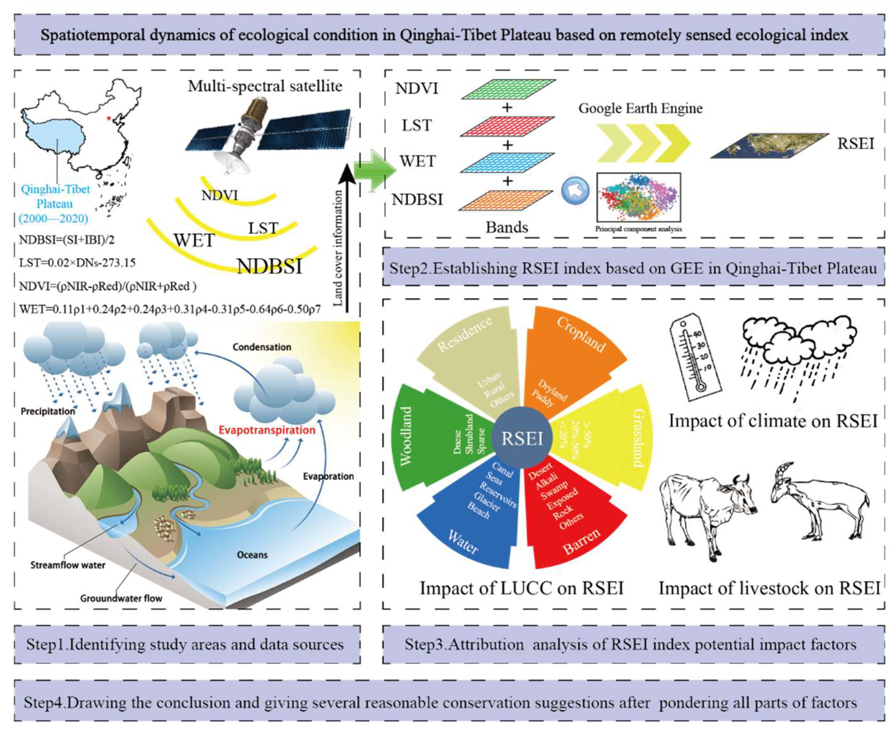
2. Materials and Methods
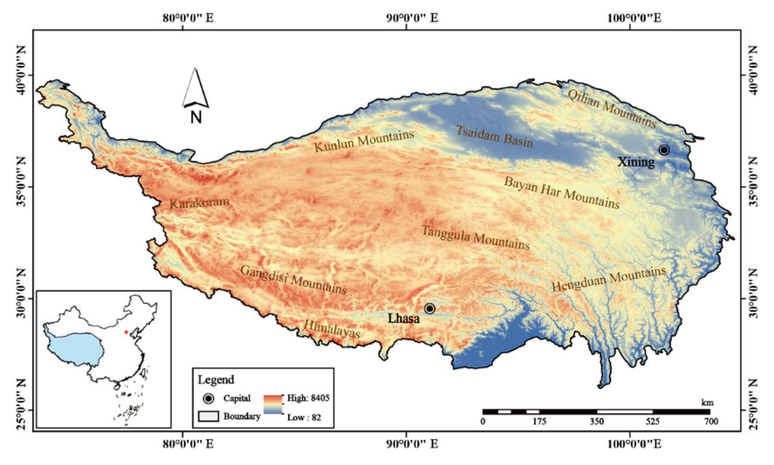
2.1. Study Site
2.2. Data and Source
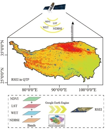
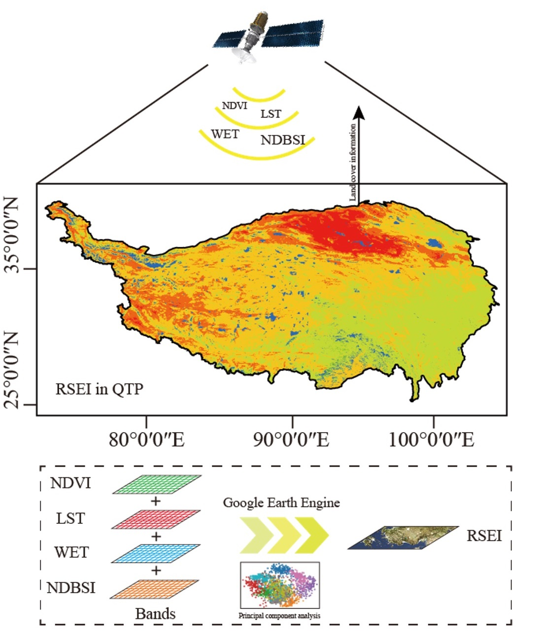
2.3. RSEI
2.4. Data Processing
2.5. Trend Analysis
3. Results
3.1. PCA
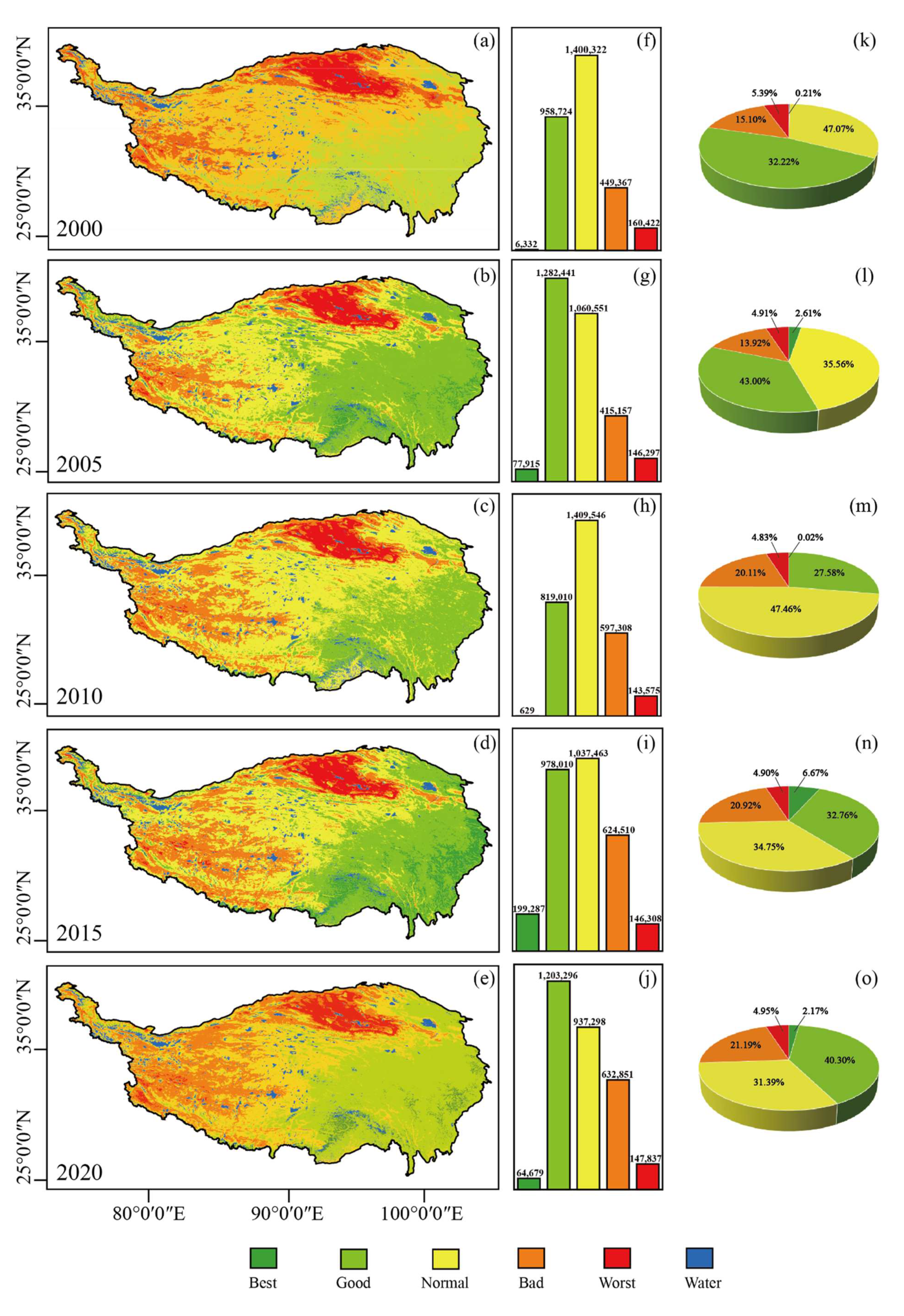
3.2. RSEI
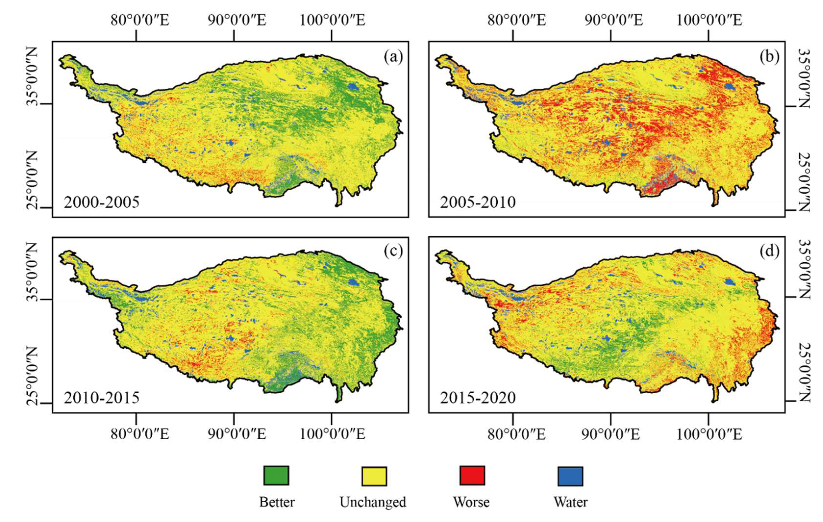
3.3. Trend Analysis
4. Discussion
4.1. Drivers of RSEI Dynamics in QTP
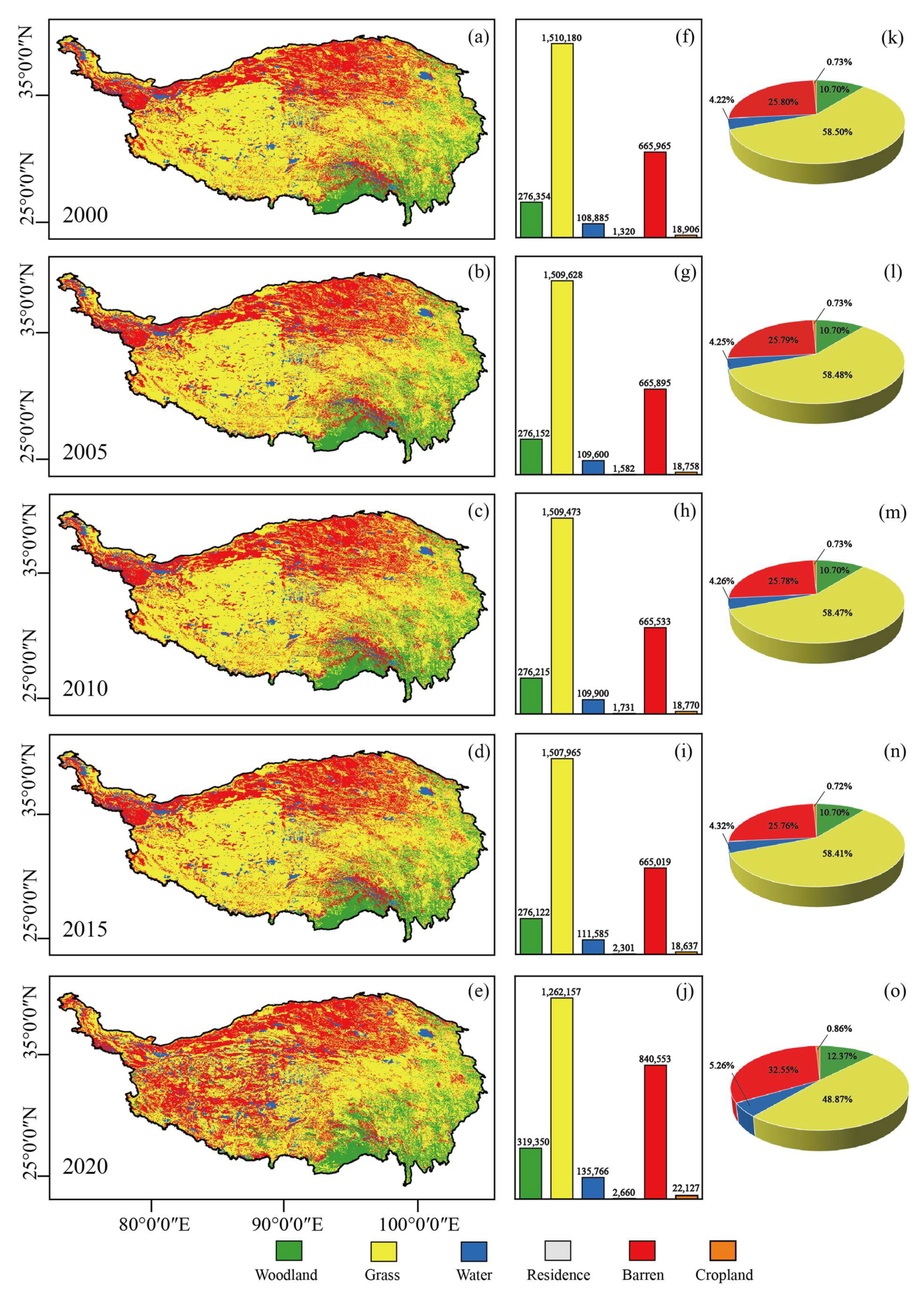
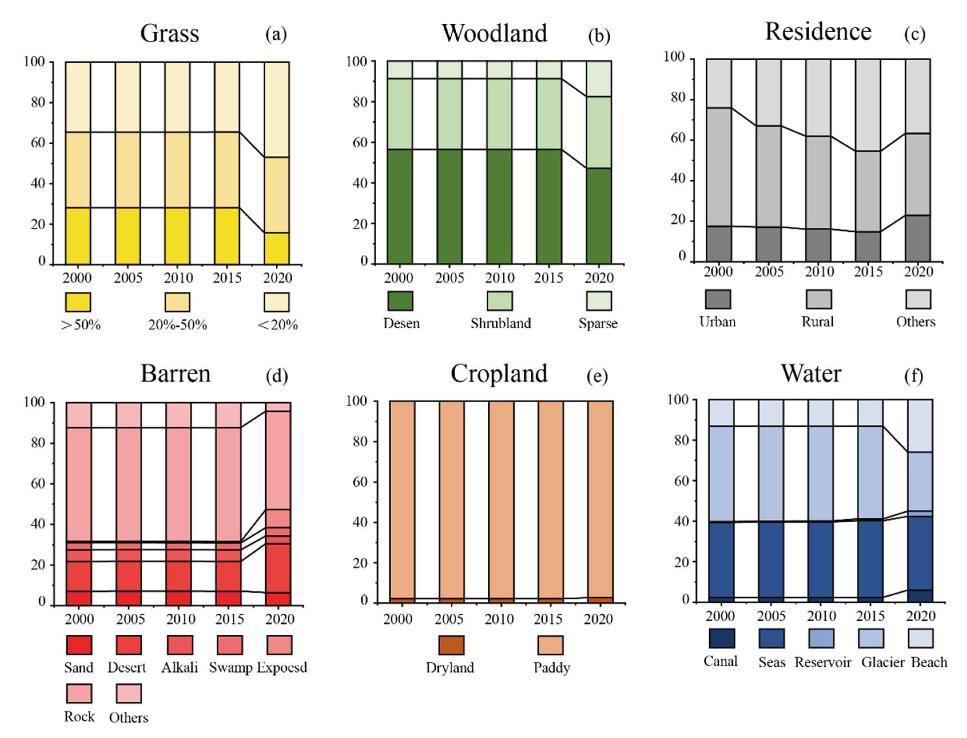
4.1.1. LUCC
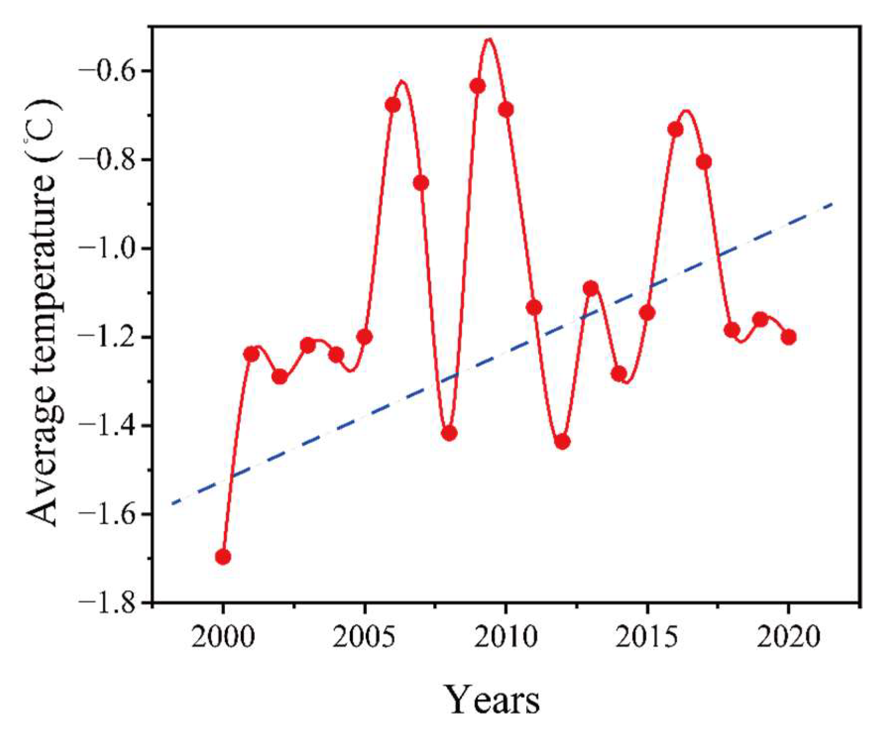
4.1.2. Temperature
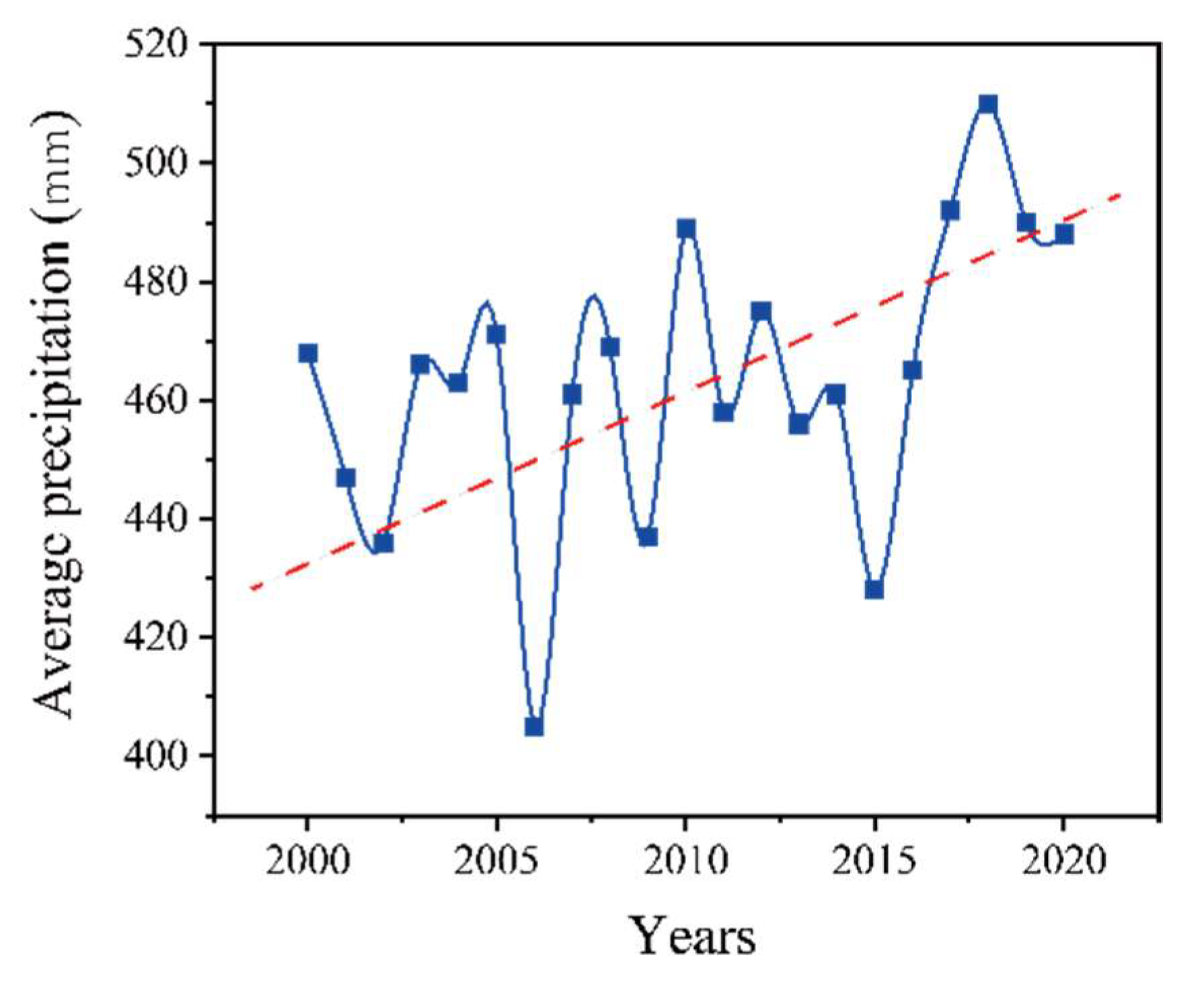
4.1.3. Precipitation
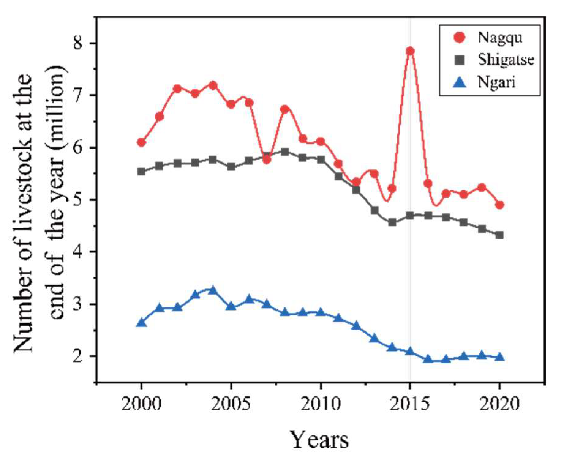
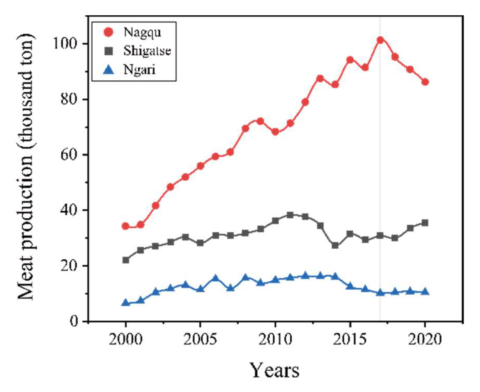
4.1.4. Grazing
4.2. Impact of Human Activities on RSEI
4.3. Uncertainty Analysis
5. Conclusions
- (1)
- The ecological condition and environmental quality in the QTP shows a long-term increasing trend, despite the annual fluctuation. Ecological recovery first occurred in 2000–2005, during which the ecological conditions of the whole area increased greatly. Nevertheless, there was a localized decrease in the central area during 2005–2010. The second period of ecological recovery happened during 2010–2015, with sporadic areas of degradation in the southwest. The second small-scale ecological degradation occurred during 2015–2020.
- (2)
- The significant ecological recovery and subsequent stability of Tsaidam Basin are the direct effects of the conservation activities. The region should continue to implement conservation measures to prevent ecological degradation. The ecological degradation of the central region during 2005–2010 was caused by the increase in temperature and the decrease in precipitation. Ecological degradation during 2015–2020 was dominated by changes in LUCC, due to grass degradation and decreasing vegetation coverage, due to overgrazing in the southwest. More restricted grazing policies should be implemented in this area to ensure a sustainable grazing industry. The comparison of the magnitude of the two periods of ecological degradation suggested that the influence of natural factors is greater. Human factors are related to the distribution characteristics of the region’s vast population.
Author Contributions
Funding
Data Availability Statement
Conflicts of Interest
References
- Song, W.; Song, W.; Gu, H.; Li, F. Progress in the Remote Sensing Monitoring of the Ecological Environment in Mining Areas. Int. J. Environ. Res. Public Health 2020, 17, 1846. [Google Scholar] [CrossRef] [PubMed]
- Rees, W.E. Ecological footprints and appropriated carrying capacity: What urban economics leaves out. Environ. Urban. 2016, 4, 121–130. [Google Scholar] [CrossRef]
- Lu, H.; Wu, N.; Liu, K.-B.; Zhu, L.; Yang, X.; Yao, T.; Wang, L.; Li, Q.; Liu, X.; Shen, C.; et al. Modern pollen distributions in Qinghai-Tibetan Plateau and the development of transfer functions for reconstructing Holocene environmental changes. Quat. Sci. Rev. 2011, 30, 279–280, 293. [Google Scholar] [CrossRef]
- Musaoglu, N.; Gurel, M.; Ulugtekin, N.; Tanik, A.; Seker, D.Z. Use of remotely sensed data for analysis of land-use change in a highly urbanized district of mega city, Istanbul. Environ. Sci. Health A Toxicol. Hazard Substance Environ. Eng. 2006, 41, 2057–2069. [Google Scholar] [CrossRef] [PubMed]
- Panwar, N.L.; Kaushik, S.C.; Kothari, S. Role of renewable energy sources in environmental protection: A review. Renew. Sustain. Energy Rev. 2011, 15, 1513–1524. [Google Scholar] [CrossRef]
- Kandziora, M.; Burkhard, B.; Müller, F. Interactions of ecosystem properties, ecosystem integrity and ecosystem service indicators—A theoretical matrix exercise. Ecol. Indic. 2013, 28, 54–78. [Google Scholar] [CrossRef]
- Stoll, S.; Frenzel, M.; Burkhard, B.; Adamescu, M.; Augustaitis, A.; Baeßler, C.; Bonet-García, F.; Carranza, M.L.; Cazacu, C.; Cosor, G.L.; et al. Assessment of ecosystem integrity and service gradients across Europe using the LTER Europe network. Ecol. Model. 2015, 295, 75–87. [Google Scholar] [CrossRef]
- Vennemo, H.; Aunan, K.; Lindhjem, H.; Seip, H.M. Environmental Pollution in China: Status and Trends. Rev. Environ. Econ. Policy 2009, 3, 209–230. [Google Scholar] [CrossRef]
- Gu, S.; Tang, Y.; Cui, X.; Kato, T.; Du, M.; Li, Y.; Zhao, X. Energy exchange between the atmosphere and a meadow ecosystem on the Qinghai–Tibetan Plateau. Agric. For. Meteorol. 2005, 129, 175–185. [Google Scholar] [CrossRef]
- Oliver, T.H.; Heard, M.S.; Isaac, N.J.B.; Roy, D.B.; Procter, D.; Eigenbrod, F.; Freckleton, R.P.; Hector, A.L.; Orme, C.D.L.; Petchey, O.; et al. Biodiversity and Resilience of Ecosystem Functions. Trends Ecol. Evol. 2015, 30, 673–684. [Google Scholar] [CrossRef] [Green Version]
- Roche, P.K.; Campagne, C.S. From ecosystem integrity to ecosystem condition: A continuity of concepts supporting different aspects of ecosystem sustainability. Curr. Opin. Environ. Sustain. 2017, 29, 63–68. [Google Scholar] [CrossRef]
- Reza, M.I.H.; Abdullah, S.A. Regional Index of Ecological Integrity: A need for sustainable management of natural resources. Ecol. Indic. 2011, 11, 220–229. [Google Scholar] [CrossRef]
- Willis, K.S. Remote sensing change detection for ecological monitoring in United States protected areas. Biol. Conserv. 2015, 182, 233–242. [Google Scholar] [CrossRef]
- Leo, G.D.; Levin, S. The multifaceted aspects of ecosystem integrity. Ecol. Soc. 1997, 1. Available online: https://www.jstor.org/stable/26271649 (accessed on 14 June 2022).
- Zampella, R.A.; Bunnell, J.F.; Laidic, K.J.; Procopio, N.A. Using multiple indicators to evaluate the ecological integrity of a coastal plain stream system. Ecol. Indic. 2006, 6, 644–663. [Google Scholar] [CrossRef]
- Müller, F.; Bicking, S.; Ahrendt, K.; Bac, D.K.; Blindow, I.; Fürst, C.; Haase, P.; Kruse, M.; Kruse, T.; Ma, L.; et al. Assessing ecosystem service potentials to evaluate terrestrial, coastal and marine ecosystem types in Northern Germany—An expert-based matrix approach. Ecol. Indic. 2020, 112, 106–116. [Google Scholar] [CrossRef]
- Ellis, E.C.; Wang, H.; Xiao, H.S.; Peng, K.; Liu, X.P.; Li, S.C.; Ouyang, H.; Cheng, X.; Yang, L.Z. Measuring long-term ecological changes in densely populated landscapes using current and historical high resolution imagery. Remote Sens. Environ. 2006, 100, 457–473. [Google Scholar] [CrossRef]
- Borja, A.; Ranasinghe, A.; Weisberg, S.B. Assessing ecological integrity in marine waters, using multiple indices and ecosystem components: Challenges for the future. Mar. Pollut. Bull. 2009, 59, 1–4. [Google Scholar] [CrossRef]
- Grantham, H.S.; Duncan, A.; Evans, T.D.; Jones, K.R.; Beyer, H.L.; Schuster, R.; Walston, J.; Ray, J.C.; Robinson, J.G.; Callow, M.; et al. Anthropogenic modification of forests means only 40% of remaining forests have high ecosystem integrity. Nat. Commun. 2020, 11, 5978. [Google Scholar] [CrossRef]
- Carlson, T.N.; Traci Arthur, S. The impact of land use—Land cover changes due to urbanization on surface microclimate and hydrology: A satellite perspective. Glob. Planet. Change 2000, 25, 49–65. [Google Scholar] [CrossRef]
- Mcdowell, N.G.; Coops, N.C.; Beck, P.S.; Chambers, J.Q.; Gangodagamage, C.; Hicke, J.A.; Huang, C.-Y.; Kennedy, R.; Krofcheck, D.J.; Litvak, L.; et al. Global satellite monitoring of climate-induced vegetation disturbances. Trends Plant Sci. 2015, 20, 114–123. [Google Scholar] [CrossRef] [PubMed] [Green Version]
- Decker, K.L.; Pocewicz, A.; Harju, S.; Holloran, M.; Fink, M.M.; Toombs, T.P.; Johnston, D.B. Landscape disturbance models consistently explain variation in ecological integrity across large landscapes. Ecosphere 2017, 8, e01775. [Google Scholar] [CrossRef]
- Hu, X.; Xu, H. A new remote sensing index for assessing the spatial heterogeneity in urban ecological quality: A case from Fuzhou City, China. Ecol. Indic. 2018, 89, 11–21. [Google Scholar] [CrossRef]
- Liu, Y.; Bao, Q.; Duan, A.; Qian, Z.; Wu, G. Recent progress in the impact of the Tibetan Plateau on climate in China. Adv. Atmos. Sci. 2007, 24, 1060–1076. [Google Scholar] [CrossRef]
- Li, Q.; Zhang, C.; Shen, Y.; Jia, W.; Li, J. Quantitative assessment of the relative roles of climate change and human activities in desertification processes on the Qinghai-Tibet Plateau based on net primary productivity. Catena 2016, 147, 789–796. [Google Scholar] [CrossRef]
- Chen, B.; Zhang, X.; Tao, J.; Wu, J.; Wang, J.; Shi, P.; Zhang, Y.-J.; Yu, C. The impact of climate change and anthropogenic activities on alpine grassland over the Qinghai-Tibet Plateau. Agric. For. Meteorol. 2014, 189/190, 11–18. [Google Scholar] [CrossRef]
- Wang, G.; Bai, W.; Li, N.; Hu, H. Climate changes and its impact on tundra ecosystem in Qinghai-Tibet Plateau, China. Clim. Change 2010, 106, 463–482. [Google Scholar] [CrossRef]
- Zhou, S.; Wang, X.; Wang, J.; Xu, L. A preliminary study on timing of the oldest Pleistocene glaciation in Qinghai–Tibetan Plateau. Quat. Int. 2006, 154–155, 44–51. [Google Scholar] [CrossRef]
- Wang, S.; Guo, L.; He, B.; Lyu, Y.; Li, T. The stability of Qinghai-Tibet Plateau ecosystem to climate change. Phys. Chem. Earth Parts A/B/C 2020, 115, 102827. [Google Scholar] [CrossRef]
- Scholes, R.J.; Mace, G.M.; Turner, W.; Geller, G.N.; Jürgens, N.; Larigauderie, A.; Muchoney, D.; Walther, B.A.; Mooney, H.A. Toward a global biodiversity observing system. Science 2008, 321, 1044–1045. [Google Scholar] [CrossRef]
- Qian, W.; Lin, X.; Zhu, Y.; Fu, J. Climatic regime shift and decadal anomalous events in China. Clim. Change 2007, 84, 167–189. [Google Scholar] [CrossRef]
- Liu, X.; Lai, Z.; Fan, Q.; Long, H.; Sun, Y. Timing for high lake levels of Qinghai Lake in the Qinghai-Tibetan Plateau since the Last Interglaciation based on quartz OSL dating. Quat. Geochronol. 2010, 5, 218–222. [Google Scholar] [CrossRef]
- Kato, T.; Tang, Y.; Gu, S.; Hirota, M.; Du, M.; Li, Y.; Zhao, X. Temperature and biomass influences on interannual changes in CO2 exchange in an alpine meadow on the Qinghai-Tibetan Plateau. Glob. Change Biol. 2006, 12, 1285–1298. [Google Scholar] [CrossRef]
- Rui, Y.; Wang, S.; Xu, Z.; Wang, Y.; Chen, C.; Zhou, X.; Kang, X.; Lu, S.; Hu, Y.; Lin, Q.; et al. Warming and grazing affect soil labile carbon and nitrogen pools differently in an alpine meadow of the Qinghai–Tibet Plateau in China. J. Soils Sediments 2011, 11, 903–914. [Google Scholar] [CrossRef]
- Nan, Z.; Li, S.; Cheng, G. Prediction of permafrost distribution on the Qinghai-Tibet Plateau in the next 50 and 100 years. Sci. China Ser. D Earth Sci. 2005, 48, 797–804. [Google Scholar] [CrossRef]
- Chen, J.; Jönsson, P.; Tamura, M.; Gu, Z.; Matsushita, B.; Eklundh, L. A simple method for reconstructing a high-quality NDVI time-series data set based on the Savitzky–Golay filter. Remote Sens. Environ. 2004, 91, 332–344. [Google Scholar] [CrossRef]
- Benali, A.; Carvalho, A.C.; Nunes, J.P.; Carvalhais, N.; Santos, A. Estimating air surface temperature in Portugal using MODIS LST data. Remote Sens. Environ. 2012, 124, 108–121. [Google Scholar] [CrossRef]
- Yang, Z.; Ouyang, H.; Zhang, X.; Xu, X.; Zhou, C.; Yang, W. Spatial variability of soil moisture at typical alpine meadow and steppe sites in the Qinghai-Tibetan Plateau permafrost region. Environ. Earth Sci. 2010, 63, 477–488. [Google Scholar] [CrossRef]
- Huete, A.R. A Soil-Adjusted Vegetation Index (SAVI). Remote Sens. Environ. 1988, 25, 295–309. [Google Scholar] [CrossRef]
- Yang, X.; Meng, F.; Fu, P.; Zhang, Y.; Liu, Y. Spatiotemporal change and driving factors of the Eco-Environment quality in the Yangtze River Basin from 2001 to 2019. Ecol. Indic. 2021, 131, 108214. [Google Scholar] [CrossRef]
- Sharma, S.; Swayne, D.A.; Obimbo, C. Trend analysis and change point techniques: A survey. Energy Ecol. Environ. 2016, 1, 123–130. [Google Scholar] [CrossRef] [Green Version]
- Hirsch, R.M.; Slack, J.R.; Smith, R.A. Techniques of trend analysis for monthly water quality data. Water Resour. Res. 1982, 18, 107–121. [Google Scholar] [CrossRef]
- Chowdhury, T.R.; Ahmed, Z.; Islam, S.; Akter, S.; Ambinakudige, S.; Kung, H.-T. Trend Analysis and Simulation of Human Vulnerability Based on Physical Factors of Riverbank Erosion Using RS and GIS. Earth Syst. Environ. 2021, 5, 709–723. [Google Scholar] [CrossRef]
- Li, X.R.; Jia, X.H.; Dong, G.R. Influence of desertification on vegetation pattern variations in the cold semi-arid grasslands of Qinghai-Tibet Plateau, North-west China. J. Arid. Environ. 2006, 64, 505–522. [Google Scholar] [CrossRef]
- Cao, J.; Yeh, E.T.; Holden, N.M.; Yang, Y.; Du, G. The effects of enclosures and land-use contracts on rangeland degradation on the Qinghai–Tibetan plateau. J. Arid. Environ. 2013, 97, 3–8. [Google Scholar] [CrossRef]
- Wen, L.; Dong, S.; Li, Y.; Li, X.; Shi, J.; Wang, Y.; Liu, D.; Ma, Y. Effect of degradation intensity on grassland ecosystem services in the alpine region of Qinghai-Tibetan Plateau, China. PLoS ONE 2013, 8, e58432. [Google Scholar] [CrossRef] [PubMed]
- Lambin, E.F.; Baulies, X.; Bockstael, N.; Fisher, G.; Krug, T.; Leemans, R.; Moran, E.F.; Rindfuss, R.R.; Sato, Y.; Skole, D.; et al. Land-Use and Land-Cover Change (LUCC): Implementation Strategy. Environ. Policy Collect. 1999, 126. Available online: https://digital.library.unt.edu/ark:/67531/metadc12005/ (accessed on 14 June 2022).
- Song, X.; Yang, G.; Yan, C.; Duan, H.; Liu, G.; Zhu, Y. Driving forces behind land use and cover change in the Qinghai-Tibetan Plateau: A case study of the source region of the Yellow River, Qinghai Province, China. Environ. Earth Sci. 2009, 59, 793–801. [Google Scholar] [CrossRef]
- Ou, X.; Lai, Z.; Zhou, S.; Zeng, L. Timing of glacier fluctuations and trigger mechanisms in eastern Qinghai–Tibetan Plateau during the late Quaternary. Quat. Res. 2017, 81, 464–475. [Google Scholar] [CrossRef]
- Xue, X.; Guo, J.; Han, B.; Sun, Q.; Liu, L. The effect of climate warming and permafrost thaw on desertification in the Qinghai–Tibetan Plateau. Geomorphology 2009, 108, 182–190. [Google Scholar] [CrossRef]
- Wu, Q.; Zhang, T. Recent permafrost warming on the Qinghai-Tibetan Plateau. J. Geophys. Res. 2008, 113, D13. [Google Scholar] [CrossRef]
- You, Q.; Kang, S.; Aguilar, E.; Yan, Y. Changes in daily climate extremes in the eastern and central Tibetan Plateau during 1961–2005. J. Geophys. Res. 2008, 113, D7. [Google Scholar] [CrossRef] [Green Version]
- Li, Y.; Li, D.; Yang, S.; Liu, C.; Zhong, A.; Li, Y. Characteristics of the precipitation over the eastern edge of the Tibetan Plateau. Meteorol. Atmos. Phys. 2009, 106, 49–56. [Google Scholar] [CrossRef]
- Dong, L.; Li, J.; Sun, J.; Yang, C. Soil degradation influences soil bacterial and fungal community diversity in overgrazed alpine meadows of the Qinghai-Tibet Plateau. Sci. Rep. 2021, 11, 11538. [Google Scholar] [CrossRef]
- Wu, G.-L.; Du, G.-Z.; Liu, Z.-H.; Thirgood, S. Effect of fencing and grazing on a Kobresia-dominated meadow in the Qinghai-Tibetan Plateau. Plant Soil 2008, 319, 115–126. [Google Scholar] [CrossRef]
- Long, R.J.; Ding, L.M.; Shang, Z.H.; Guo, X. The yak grazing system on the Qinghai-Tibetan plateau and its status. Rangel. J. 2008, 30, 241–246. [Google Scholar] [CrossRef]


| Index | Product | Spatial Resolution | Temporal Resolution | Level |
|---|---|---|---|---|
| NDVI | MOD13A1 | 1000 m | 16 d | L3 |
| LST | MOD11A2 | 1000 m | 8 d | L3 |
| WET | MOD09A1 | 500 m | 8 d | L3 |
| NDBSI | MOD09A1 | 500 m | 8 d | L3 |
| Index | Years | ||||
|---|---|---|---|---|---|
| 2000 | 2005 | 2010 | 2015 | 2020 | |
| NDVI | 0.4809 | 0.6411 | 0.7508 | 0.6945 | 0.6742 |
| LST | −0.8702 | −0.7559 | −0.6436 | −0.703 | −0.6662 |
| WET | 0.106 | 0.1323 | 0.1486 | 0.1534 | 0.3189 |
| NDBSI | −0.0004 | −0.0001 | −0.0001 | −0.0009 | −0.001 |
| EV (pc1) | 0.0481 | 0.0572 | 0.0562 | 0.0572 | 0.0671 |
| EV (pc2) | 0.0359 | 0.0319 | 0.032 | 0.0239 | 0.0249 |
| ECR (pc1%) | 56.1 | 62.54 | 61.75 | 68.25 | 66.73 |
| ECR (pc2%) | 41.92 | 34.87 | 35.12 | 28.51 | 24.77 |
| Index | 2000–2005 | 2005–2010 | 2010–2015 | 2015–2020 |
|---|---|---|---|---|
| Better | 20.85% | 1.21% | 21.93% | 10.70% |
| Unchanged | 74.85% | 71.24% | 73.18% | 77.57% |
| Worse | 4.31% | 27.56% | 4.89% | 11.74% |
| LUCC (%) | Years | |||||
|---|---|---|---|---|---|---|
| I | II | 2000 | 2005 | 2010 | 2015 | 2020 |
| Woodland | Dense | 56.39% | 56.36% | 56.38% | 56.38% | 47.20% |
| Shrubland | 34.85% | 34.87% | 34.88% | 34.88% | 35.25% | |
| Sparse | 8.75% | 8.77% | 8.74% | 8.74% | 17.55% | |
| Grass | >50% | 28.10% | 28.11% | 28.12% | 28.13% | 15.71% |
| 20–50% | 37.34% | 37.34% | 37.34% | 37.34% | 37.23% | |
| <20% | 34.56% | 34.55% | 34.54% | 34.52% | 47.06% | |
| Water | Canal | 2.37% | 2.36% | 2.35% | 2.37% | 5.96% |
| Seas | 36.98% | 37.24% | 37.30% | 37.82% | 36.38% | |
| Reservoir | 0.42% | 0.44% | 0.46% | 0.95% | 2.56% | |
| Glacier | 47.12% | 46.80% | 46.65% | 45.76% | 29.15% | |
| Beach | 13.10% | 13.16% | 13.24% | 13.09% | 25.96% | |
| Residence | Urban | 17.58% | 34.47% | 16.18% | 14.86% | 22.97% |
| Rural | 58.41% | 49.87% | 45.81% | 39.72% | 40.45% | |
| Others | 24.02% | 32.93% | 38.01% | 45.42% | 36.58% | |
| Barren | Sand | 7.12% | 7.22% | 7.22% | 7.19% | 6.42% |
| Desert | 14.68% | 14.67% | 14.68% | 14.65% | 24.12% | |
| Alkali | 5.77% | 5.73% | 5.70% | 5.73% | 3.78% | |
| Swamp | 3.46% | 3.41% | 3.40% | 3.37% | 4.15% | |
| Exposed | 0.73% | 0.73% | 0.72% | 0.72% | 8.79% | |
| Rock | 56.02% | 56.02% | 56.07% | 56.15% | 48.54% | |
| Others | 12.22% | 12.23% | 12.21% | 12.19% | 4.18% | |
| Cropland | Dryland | 2.27% | 2.27% | 2.26% | 2.27% | 2.73% |
| Paddy | 97.73% | 97.73% | 97.74% | 97.73% | 97.27% | |
Publisher’s Note: MDPI stays neutral with regard to jurisdictional claims in published maps and institutional affiliations. |
© 2022 by the authors. Licensee MDPI, Basel, Switzerland. This article is an open access article distributed under the terms and conditions of the Creative Commons Attribution (CC BY) license (https://creativecommons.org/licenses/by/4.0/).
Share and Cite
Cao, J.; Wu, E.; Wu, S.; Fan, R.; Xu, L.; Ning, K.; Li, Y.; Lu, R.; Xu, X.; Zhang, J.; et al. Spatiotemporal Dynamics of Ecological Condition in Qinghai-Tibet Plateau Based on Remotely Sensed Ecological Index. Remote Sens. 2022, 14, 4234. https://doi.org/10.3390/rs14174234
Cao J, Wu E, Wu S, Fan R, Xu L, Ning K, Li Y, Lu R, Xu X, Zhang J, et al. Spatiotemporal Dynamics of Ecological Condition in Qinghai-Tibet Plateau Based on Remotely Sensed Ecological Index. Remote Sensing. 2022; 14(17):4234. https://doi.org/10.3390/rs14174234
Chicago/Turabian StyleCao, Jiaxi, Entao Wu, Shuhong Wu, Rong Fan, Lei Xu, Ke Ning, Ying Li, Ri Lu, Xixi Xu, Jian Zhang, and et al. 2022. "Spatiotemporal Dynamics of Ecological Condition in Qinghai-Tibet Plateau Based on Remotely Sensed Ecological Index" Remote Sensing 14, no. 17: 4234. https://doi.org/10.3390/rs14174234
APA StyleCao, J., Wu, E., Wu, S., Fan, R., Xu, L., Ning, K., Li, Y., Lu, R., Xu, X., Zhang, J., Yang, J., Yang, L., & Lei, G. (2022). Spatiotemporal Dynamics of Ecological Condition in Qinghai-Tibet Plateau Based on Remotely Sensed Ecological Index. Remote Sensing, 14(17), 4234. https://doi.org/10.3390/rs14174234