Article

Challenging Environments for Precise Mapping Using GNSS/INS-RTK Systems: Reasons and Analysis

The Advanced Mobility Research Institute, Kanazawa University, Kanazawa 920-1192, Japan
*
Author to whom correspondence should be addressed.
Remote Sens. 2022, 14(16), 4058; https://doi.org/10.3390/rs14164058
Submission received: 31 May 2022 / Revised: 20 July 2022 / Accepted: 15 August 2022 / Published: 19 August 2022

Abstract

:
This paper demonstrates the weakness of GNSS/INS-RTK (GIR) systems in mapping challenging environments because of obstruction and deflection of satellite signals. Thus, it emphasizes that the strategy of mapping companies to commercially provide maps using expensive GIR systems does not always work robustly. This limits the scalability of autonomous vehicle deployment in many road structures and modern cities. Accordingly, different critical environments in Tokyo have been analyzed and investigated to demonstrate the effects of the road structure complexity on the GIR map quality with highlighting the relevant reasons. Therefore, this paper is intended to be a reference to prove that the data of GIR systems cannot always be considered as ground truth and the integration of SLAM technologies into the mapping modules is very necessary to enable the levels four and five of autonomous driving.

Graphical Abstract

1. Introduction

Mapping in critical environments is very important to enable many applications of remote sensing and autonomous driving. Maps should clearly represent the environmental details and accurately localize these details in the real world. There are different sensors to densely encode environments, such as cameras in the 2D image domain to provide color and appearance and LIDAR in the 3D point cloud domain to represent shape and texture [1,2]. As maps are the main pillar for Advanced Driving Assistance Systems (ADAS) and autonomous driving, researchers and companies tend to use expensive and accurate GNSS/INS-RTK (GIR) systems to position the sensing data of environmental features in the real world [3]. This tactic allows us to safely focus on solving problems in the perception, path-planning, localization and motion controlling modules [4,5]. However, this strategy cannot be applied in challenging environments such as long tunnels, high buildings and dense trees because of obstruction and deflection of the satellite signals. Accordingly, the maps are distorted due to the contradictions in positions, especially in the revisited areas. Consequently, such maps cannot be utilized to enable safe autonomous driving, and the corresponding road structures are excluded from autonomous vehicle deployment.
There are many approaches to recover environmental representations and compensate for the GIR errors to generate precise maps, such as Simultaneous Localization and Mapping (SLAM) technologies [6,7]. SLAM-based mapping systems have sufficiently been developed and investigated in the literature, and various methods have been proposed using different implementation tactics and sensor types [8,9,10,11]. The main idea is to utilize the relationships between vehicle positions to improve low accurate trajectories. This is achieved by compensating the localization errors in the revisited areas based on matching the stationary environmental features. These compensations are integrated into a probabilistic framework with the position measurements of other techniques such as GIR and Dead Reckoning (DR) [12]. Meanwhile, the confidence of the measurements is modeled to provide the covariance errors. The estimations and the covariance errors are then mathematically incorporated into a cost function to optimize the vehicle trajectory and generate precise maps accordingly.
In the Advanced Mobility Research Institute at Kanazawa University in Japan, we investigated both strategies of using GIR and SLAM-based mapping systems to generate LIDAR maps and conduct autonomous driving in different cities and road structures [13,14]. The SLAM integration into the mapping module was considered after two years of using GIR systems when observing low capabilities to map complex roads [15]. Based on the gained lessons and the relevant experiences, we inferred that there is no common reference in the literature to illustrate the GIR systems’ weak performances and demonstrate the relevant effects on the maps. Therefore, this paper is presented to show the experimental results of generating GIR maps in different challenging traffic junctions in Japan. In addition, the map distortions are highlighted at various road segments in different patterns to provide a complete idea of the effects in the mapping domain. Furthermore, different autonomous vehicles (agents) and driving scenarios were taken into account to analyze the map quality of the same environments with different traffic flows and data collection dates. Thus, we believe that this paper can be sufficiently considered as a reference to prove the low capabilities of GIR systems to generate precise maps and the necessity to integrate SLAM technologies into the mapping modules.
The remainder of the paper is structured to provide a brief explanation in Section 2 on the map creation strategy to efficiently represent the effects of the GIR low mapping capabilities in the XYZ plane. The candidate reasons for the error occurrence and the corresponding distortion patterns in the maps are emphasized in Section 3. The experiment setups and the relevant results of generating GIR maps in different challenging environments are demonstrated in Section 4. Finally, the conclusion section in Section 5 summarizes the important points.

2. Mapping Strategy Using GNSS/INS-RTK System

LIDAR-based mapping modules can be implemented to generate different types of maps. For example, the map is explained in ref. [16] by 3D point clouds to represent the shape and feature distribution of environments. Another approach is to encode only stationary environmental features such as poles, painted landmarks, barriers, guardrails, traffic signs and so on [17,18]. This approach significantly reduces the storing size and is compatible with cloud source-based mapping systems. On the other hand, it lacks in providing dense details, especially in texture-less and feature-less environments such as highways, long tunnels and rural roads. Therefore, a mapping module can be implemented based on using the full LIDAR information of points’ xyz coordinates as well as the reflectivity values, i.e., 2.5D elevation maps [19,20,21]. The xy coordinates and the intensity values are utilized to represent the road surfaces in 2D intensity images, whereas the z coordinates are used to encode the road slopes and the particular height of each pixel in the intensity images. This approach can be placed between the above two explained methods in terms of storing size. In contrast, it provides a continuous dense representation of the roads and surrounding environments. Thus, it is very compatible with the scope of this paper to illustrate the effects of GIR systems on the maps by clearly showing the distortions using road surface intensity images in the XY plane and the elevation errors in the Z plane. We implemented and modified LIDAR-based 2.5D mapping and localization systems to conduct autonomous driving in different cities in Japan, and a technical explanation of the map creation strategy is briefly provided in the next section [19].

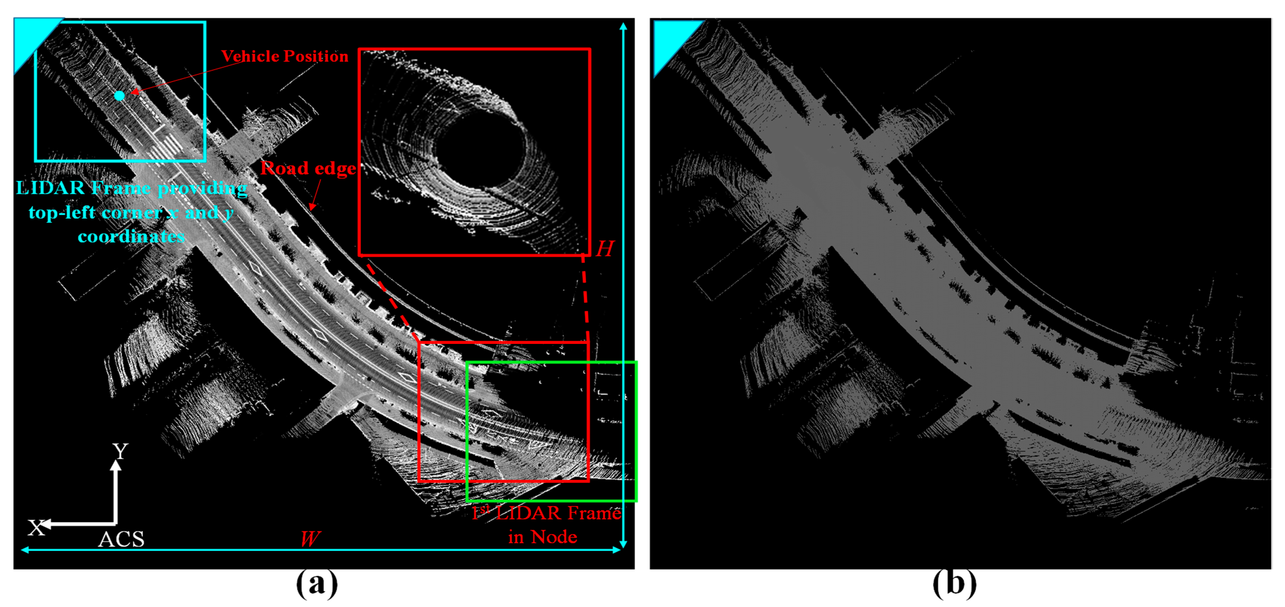
2.1. 2.5D Map Creation (Intensity and Elevation)

A LIDAR point cloud is cut at a height of 0.3 m to encode road surfaces and converted into 2D intensity and elevation frames in the image domain using a series of transformations between vehicle, LIDAR and global coordinate systems. The intensity and elevation frames are accumulated in two individual images according to the vehicle trajectory. The accumulation process is terminated when the number of the contained pixels exceeds a threshold β, and a node is accordingly added to the map, as illustrated in Figure 1. The node is identified in the Absolute Coordinate System (ACS) using the top-left corner. The xy coordinates of the corner are determined by the maximum vehicle position in XY directions inside the node’s driving area, whereas the z coordinate is obtained by averaging the non-zero pixel values in the elevation image as in Figure 1b. The accumulation process is then reset to create new nodes and extend the map size accordingly.
The node-based creation tactic is very important to divide roads into segments that relatively represent wide road surfaces. The implicit representation of the vehicle trajectory by β significantly prevents encoding a multilevel road structure in the same node, e.g., bridge and underpass road surfaces. This effectively facilitates automatically detecting, extracting and arranging the relationships between nodes, such as scanning the same, neighboring and opposite lanes in the same environments, i.e., loop-closure. Accordingly, the GIR map quality can easily be analyzed to indicate distortions based on the driving scenarios. Furthermore, this tactic enables us to study the distortions in the XY and Z planes individually and collectively. Thus, the reasons and the types of these distortions are detailed in the next section.

3. Reasons and Types of Map Distortions

Loop closures are very necessary to update environment representations and increase the road surface density, especially on highways and streets with parked vehicles. In contrast, loop closures are the main reason to produce distortions in maps because of scanning the same areas multiple times and merging these scans in ACS. The multiple scans might be combined with different global position accuracies and lead to encode the same area at different positions in the real world. Differences in the GIR accuracy occur due to receiving satellite signals of low quality because of the complexity of the road structures and the surrounding environments. For example, the urban roads with high buildings and dense trees in Figure 2 deflect the signals, whereas long tunnels obstruct them considerably. These two effects may both exist in multilevel road structures where longitudinal bridges deflect and obstruct receiving the signals in lower layers, e.g., underpass. Traffic flow may also cause reflectance and deflection of the signals, especially in closed-sky areas such as tunnels and multifloor parking lots. In addition, driving scenarios play the main role in producing distortions in the maps because of visiting areas from different directions, e.g., scanning an open-sky segment of a T-Junction and then returning via the other segment covered by dense trees as in Figure 2 (top-left image). Accordingly, the open-sky segment is distorted in the map due to the processing time to recover the signal accuracy by GIR after coming out from the dense-tree segment. Furthermore, a special spatial distortion may occur in the consistency between layers in multilevel environments in the XY plane, e.g., each layer has a different global position relative to the other layers. The layer inconsistency may considerably limit autonomous vehicle applications such as sharing traffic jam information at different layers, i.e., if the layers are not perfectly aligned in the XY plane, the opposite lanes between layers may wrongly share the same global xy coordinates as illustrated later in Figure 12d. Finally, map combination is another main and critical reason to massively distort GIR maps because of the high potential to collect mapping data by different agents, sensor configurations, environment changes, driving scenarios and traffic flows.
The map distortions in the XY plane appear in the image domain as duplications of the road surface in the lane representations and ghosting effects around the printed landmarks. Figure 3 demonstrates different distortion types in various road surfaces, structures and painted landmarks. These distortions are magnified according to the number of loop closures and the relative position errors in each closure. The effects of these deformations on the localization accuracy during autonomous driving differ according to the road surface conditions. For example, the duplication of lane lines produces multiple matching patterns with the sensory observation data, whereas the ghosting in landmarks leads to the weakening of the matching pattern.
The distortions in the Z plane appear in changing the road slopes and creating unreal bumps in the road context. The road slopes affect the calculation of roll and pitch angles, whereas the virtual bumps produce sudden changes in estimating the z vehicle position that may lead to wrong calculations of the distances to other road users [22].
The effects of the above distortions in the XY and Z planes are magnified in mapping the multilevel environments where different layers might be inconsistently structured in the GIR maps because of the wrong xy positions in ACS or wrongly encoded in the same elevation level because of the wrong z positions. This leads to a massive change in the road representation compared to the observation data and may cause traffic accidents during autonomous driving. In order to illustrate the above explanations and effects, different real experiments in mapping challenging environments in Japan by the GIR systems are demonstrated in the next chapter.

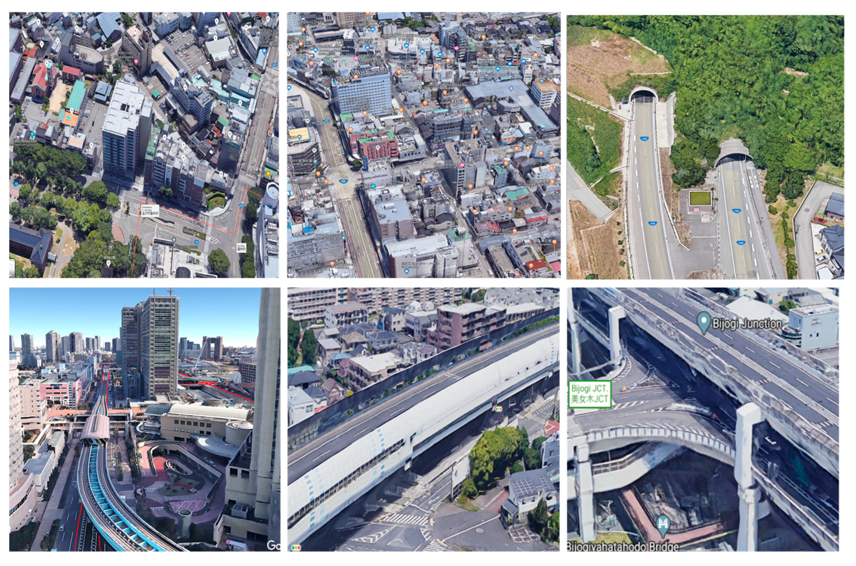
4. Challenging Environments for Mapping Using GIR Systems

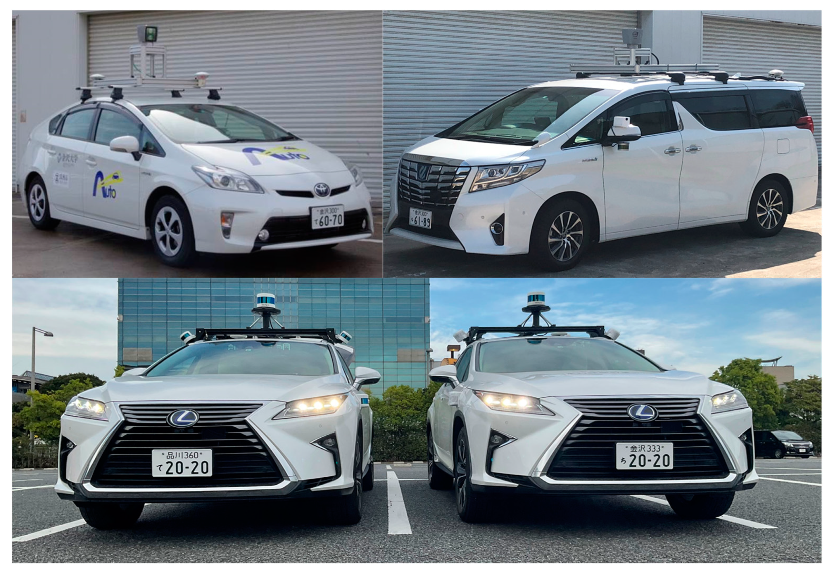
4.1. Setup and Experimental Platforms

Figure 4 shows four experimental platforms that were used to collect mapping data in different cities in Japan. These vehicles are equipped with many sensors and are usually used to conduct autonomous driving. Lexus-1 and Lexus-2 are identical and have LIDAR VLS-128-AP with 128 laser beams and a GIR system of Applanix PosLV 220, whereas Pruis is equipped with Velodyne HDL-64 S2 and Applanix PosLV 110, and Alphard possesses Velodyne HDL-64 S2 and Applanix PosLV 220.
In the data collection phase, the vehicle is manually driven to scan environments and record the GIR measurements. The measurements are offline post-processed by a special software provided by Applanix to optimize the vehicle trajectory in the real world. The software is called POSPAC and uses some optimization techniques such as Kalman Filter, closed-loop error controllers and positions smoothers to estimate the vehicle trajectory and model the position accuracy based on both IMU and GIR measurements [23,24]. The accuracy in open-sky areas is around 2~5 cm and changes considerably in the challenging road structures to be in the meter order. These accuracy estimations are illustrated in profiles along the test courses to demonstrate the relationships between the road structures and the satellite signal quality. The LIDAR point clouds are then accumulated based on the post-processed trajectories as explained in Section 2.1 to generate GIR intensity–elevation maps, i.e., 2.5D maps.
The pixel resolution in maps is 0.125 m and the number of pixels to produce a node is β = 1 M. The elevation images are stored in a float format to represent the exact height in the real world of each pixel in the intensity images. Loop closures between nodes are detected and determined based on the top-left corners in the XY plane and the IDs of sampling the nodes into sub-images [25].

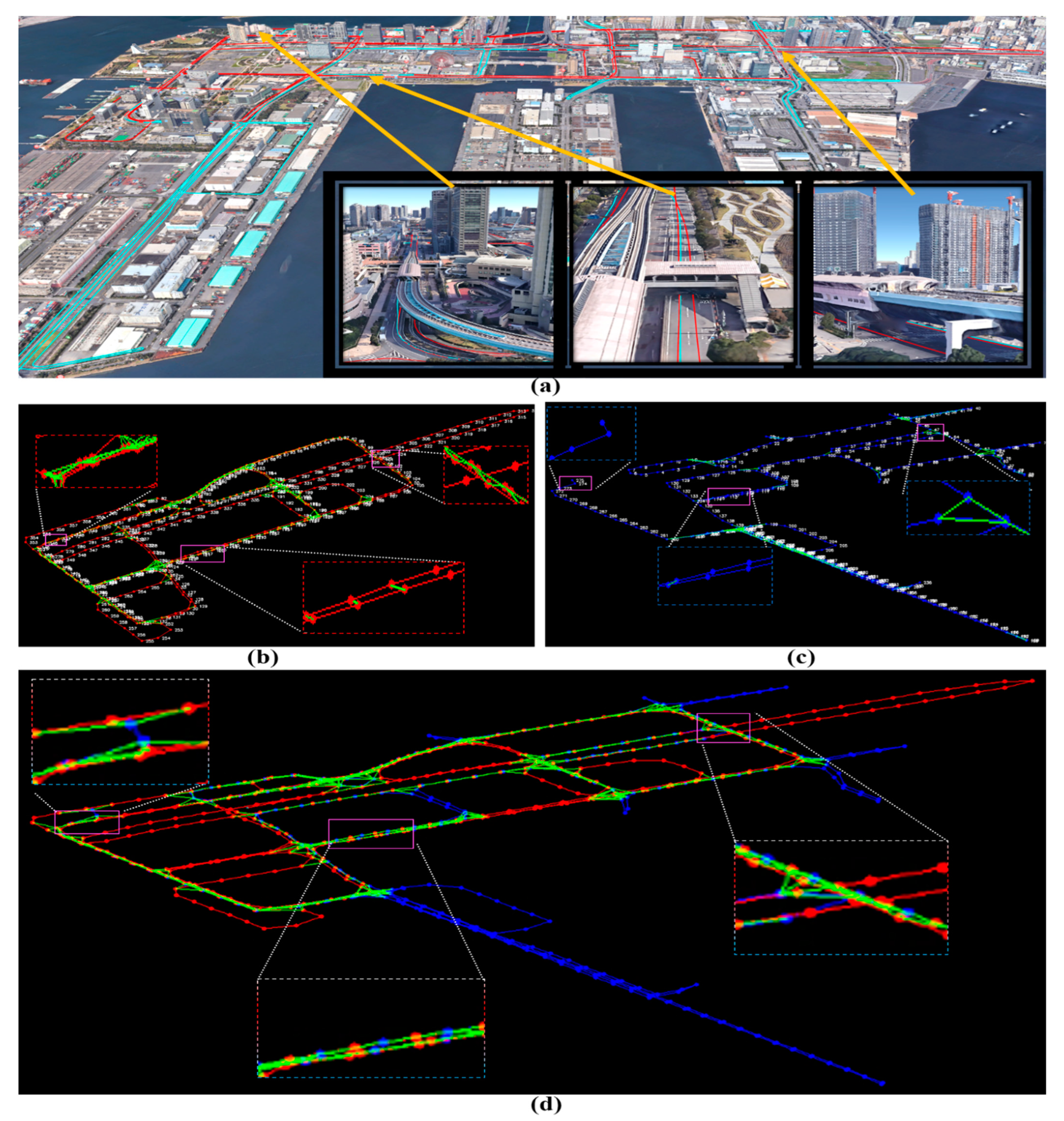
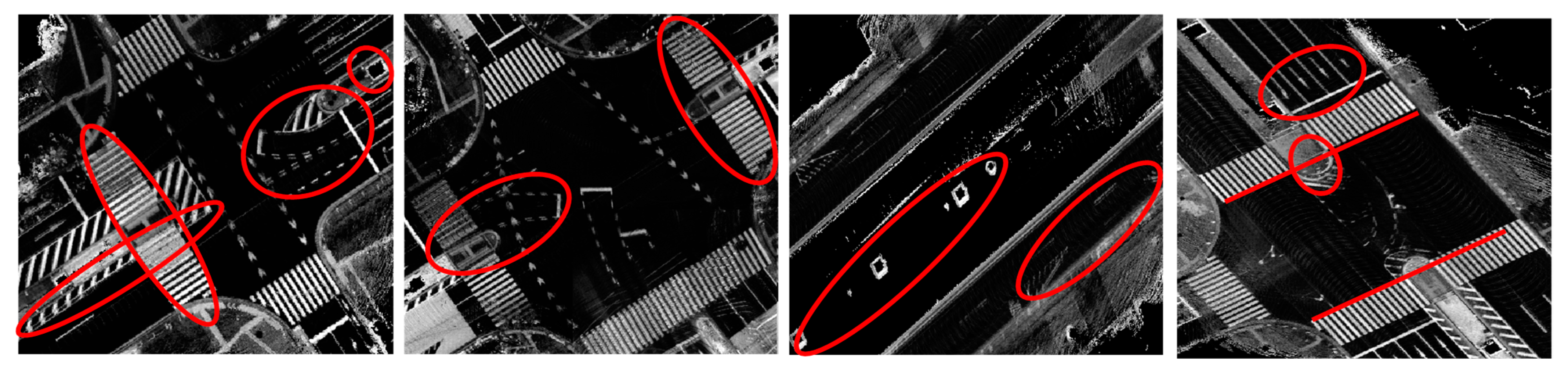
4.2. Mapping an Urban Area Using a Single Drive and a Single Agent

Urban roads in modern cities are challenging environments for mapping modules because of the surrounding high buildings and dense trees. We chose Tokyo in Japan as a test field for generating GIR maps because of the existing different complex road structures and highways as well as long longitudinal bridges and tunnels. Therefore, enabling safe autonomous driving is a very tricky and necessary demanded.
An arterial ground road in Tokyo that is fully covered by a longitudinal bridge was scanned using Lexus-2, as illustrated in Figure 5. The road allows driving in two directions, each of which has been scanned once. The number of nodes is 436, representing 46.5 km in the real world and equivalent to 39,011 LIDAR point clouds. Thus, continuous loop closures (240) mainly occurred between the two road shoulders, as indicated by the green links in Figure 5a. Figure 5b shows the GIR accuracy profile of the nodes in the re-visited areas in the X and Y directions, respectively. One can observe the huge differences between the corresponding nodes in each direction, i.e., target (Tra) and reference (Ref) nodes. Thus, the GIR map is inaccurate all the way along the course, and ghosting effects exist in different patterns of duplications of the road surface as demonstrated in Figure 5c. In addition, the GIR system has flipped the global positions of the two direct and opposite lanes in ACS at the referred area in Figure 5a. This area is indicated by the sudden changes of the GIR accuracy at the loop closure ID 196 in Figure 5b and illustrated in Figure 5c at the most right image. Accordingly, this massive wrong representation of the road structure compared to the real world may considerably drift the vehicle during autonomous driving and cause a deadly traffic accident.

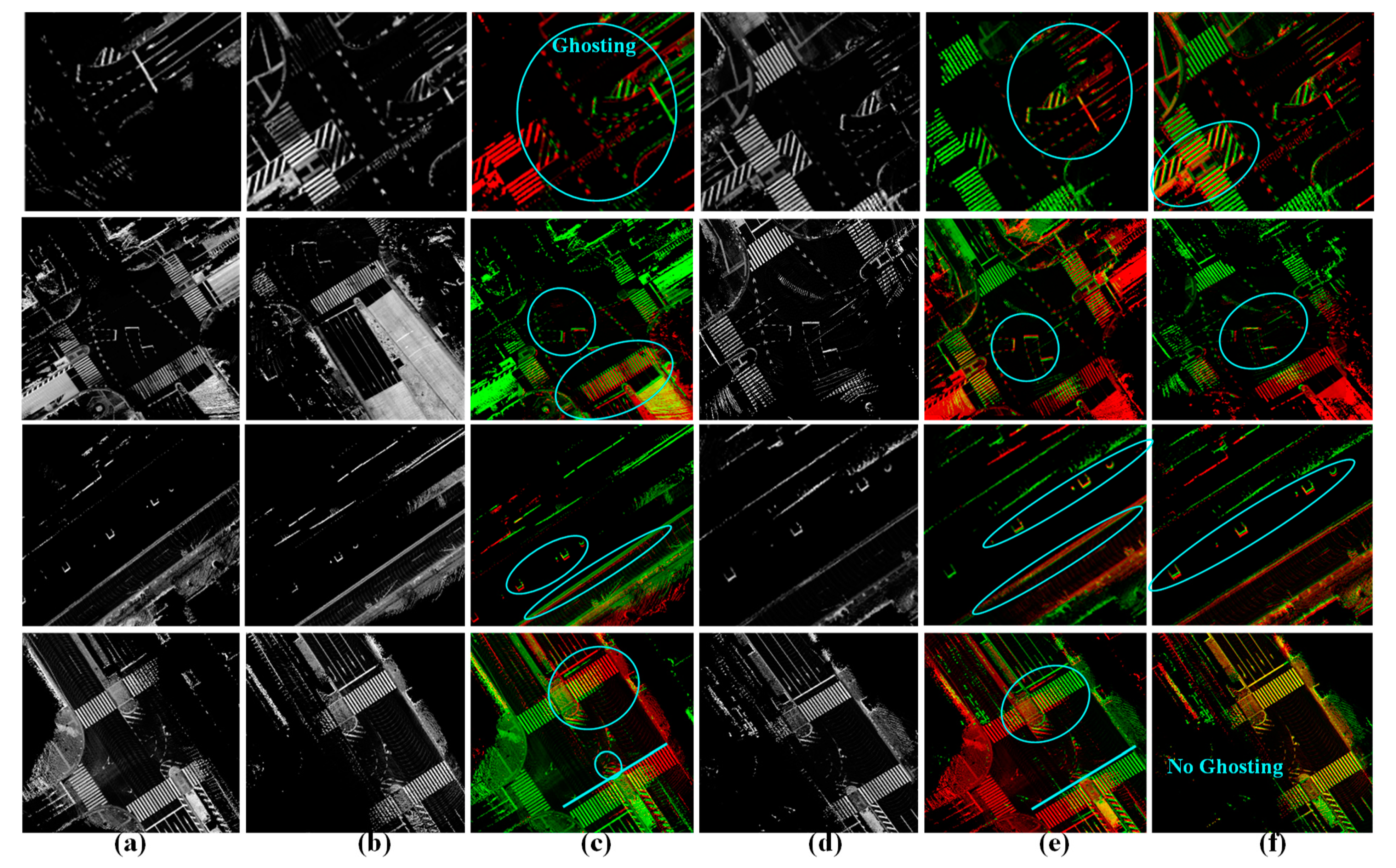
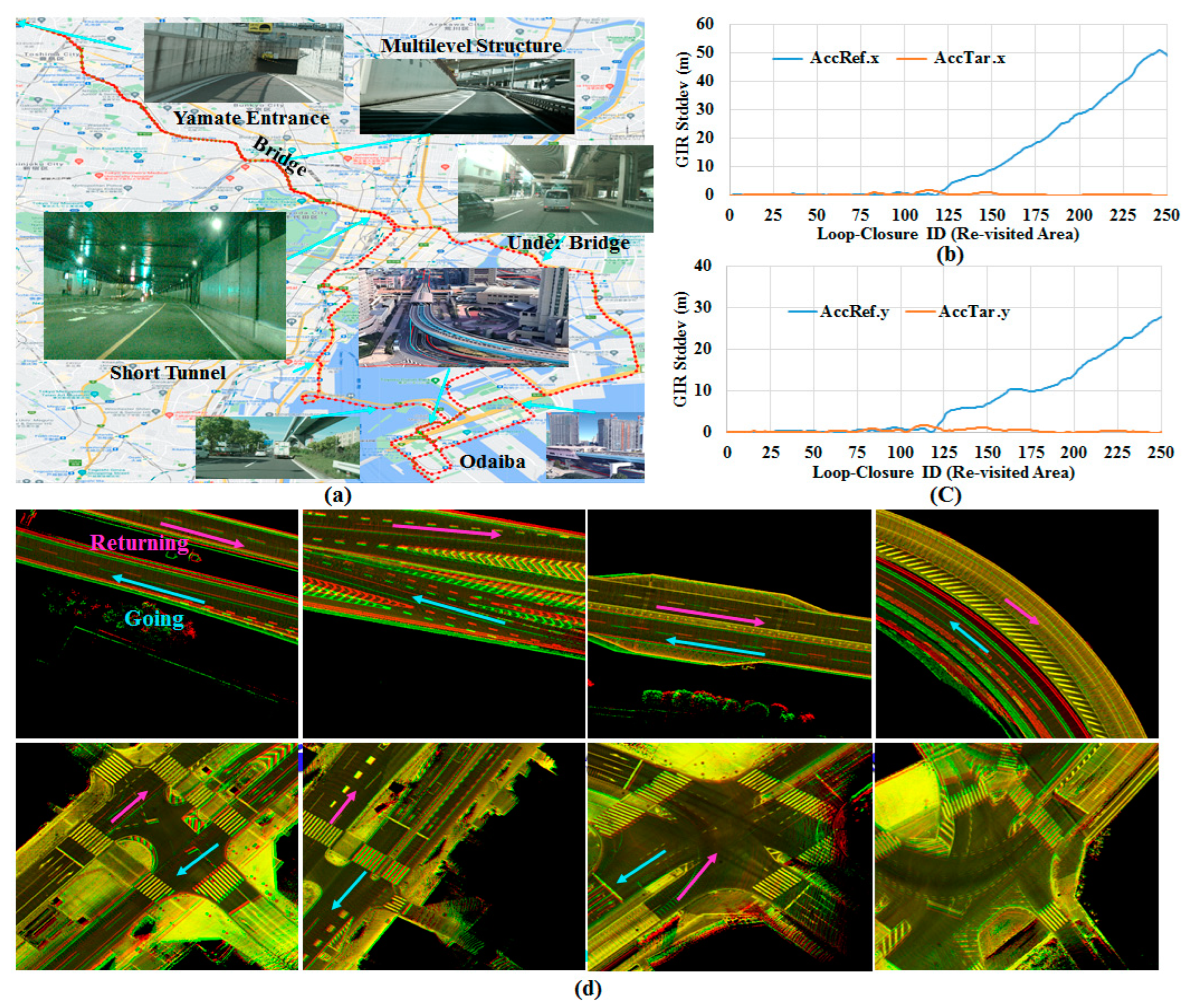
4.3. Mapping an Urban Area Using Two Drives and a Single Agent

The capability to combine maps precisely is very important in the mapping modules in order to update environments and create large-scale maps. However, this demand becomes critical in complex road structures because the GIR system might be initialized at different positions and create contradictions in the global accuracies. Tokyo’s waterfront is a challenging mapping area because it considerably reduces the quality of satellite signals due to the continuous existence of longitudinal railway bridges and tram stations as illustrated in Figure 6a. The area was scanned by Alphard car in two data collection phases on the same day as implied in Figure 6b,c. MapA is 35.6 km and consists of 364 nodes (77,423 frames) with 484 local loop-closure events. MapB is 28 km and consists of 276 nodes that are equivalent to 49,283 frames with 150 loop-closure events. Finally, the number of loop closures between two maps is 425, as demonstrated in Figure 6d.
Three road segments were mainly found to produce ghosting effects in the GIR combined map as indicated in Figure 6a, i.e., the first segment encodes an underpass road of the railway bridge with high buildings whereas the second segment is surrounded by dense trees and the third segment is fully covered by a railway station. These segments were scanned twice during the first data-collection phase (mapA) and the third scan was added in the second phase (mapB). Therefore, lateral and longitudinal deviations were produced in the road surface representation in the GIR combined map.
Figure 7 shows four samples of the three road segments in Figure 6a, demonstrating the combination of the node’s images using the GIR system. The first and second rows illustrate two areas in the first road segment to emphasize the continuity of the ghosting effects. The third and fourth rows encode areas in the second and third segments, respectively. Particularly, Figure 7a,b show road patches in nodes of the same area in mapA, i.e., local loop closures. Figure 7c shows the merging results of the two patches in Figure 7a,b based on GIR. The nodes of mapB are shown in Figure 7d and the potential map combinations with the nodes in mapA are represented in Figure 7e,f, i.e., loop closures between maps. The combined map images in Figure 7e,f show different deviations in the longitudinal and lateral directions. This implies that these areas always affect the map accuracy. In addition, it can be emphasized that the driving scenario may play a significant role in distorting the maps, i.e., driving in the same direction may yield an accurate combination as in Figure 7f (last row) because of scanning the same road structure whereas a longitudinal deviation occurred in merging the opposite lane in Figure 7c,e because of the surrounding high buildings at the right roadside as can be compared in Figure 6a (right image). Accordingly, it cannot be claimed that mapA is more precise than mapB and vice versa because both of them provided different combination patterns in the same areas. Figure 8 shows the combined GIR map images of the four road segments in Figure 7 with deformations in the landmarks and misalignments of the road lanes in the longitudinal directions.

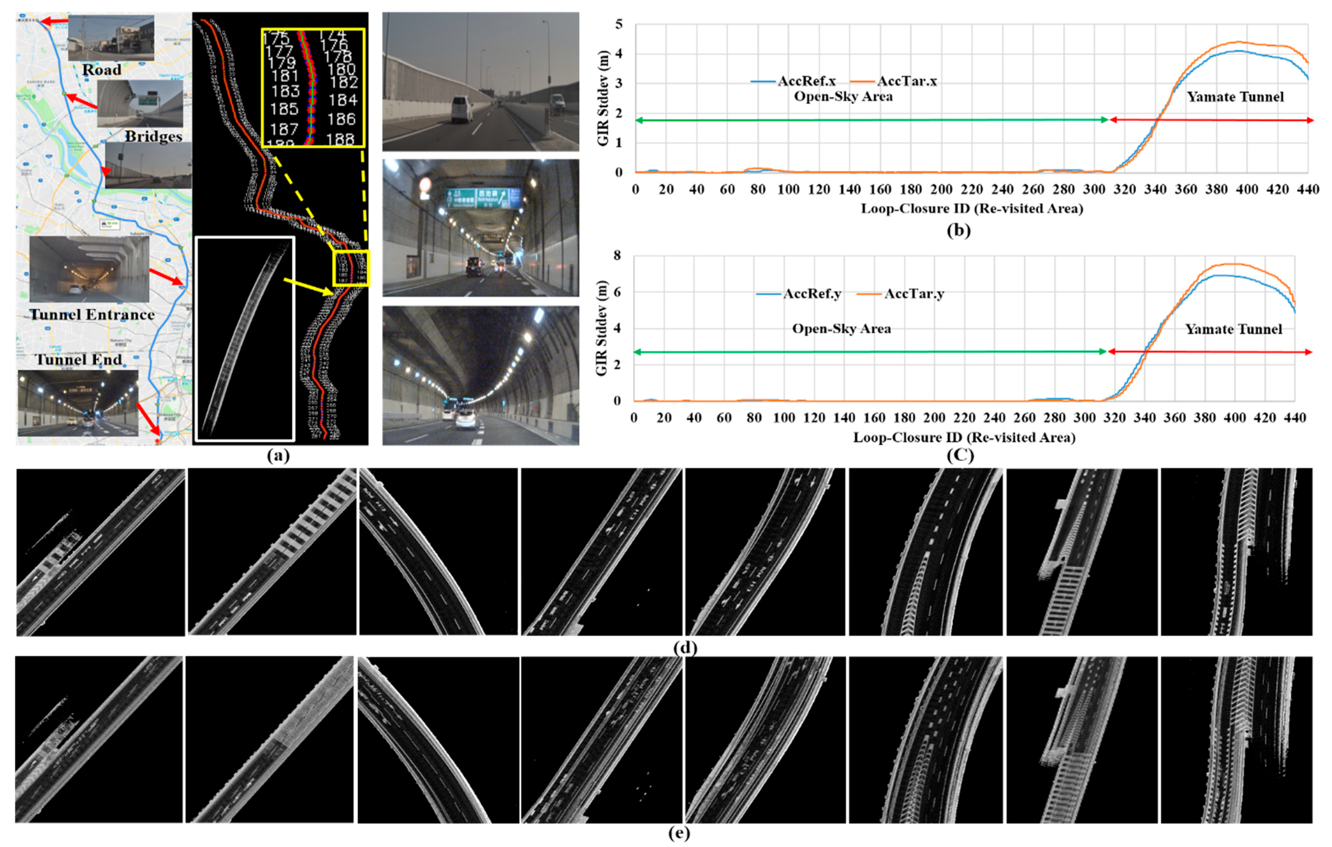
4.4. Mapping a Long Underground Tunnel Using Two Drives in the Same Driving Scenario and a Single Agent

Tunnels are an optimal environment to approximately preserve road conditions and driving scenarios fixed. This is because of the identical surrounding environments and the less availability of maneuvering such as conducting lane changes and overtaking actions. To restrict the scanning conditions, the world’s longest tunnel (Yamate Tunnel) was selected. The tunnel consists of two independent underground tubes and each tube allows a single driving direction and consists of only two lanes. The road slope in the first tube gradually changes to reach 30 m underground. Therefore, it was scanned two times using Prius as demonstrated in Figure 9a.
Figure 9b,c show the GIR accuracy profiles for the two scans in the X and Y directions. In the open-sky area, the GIR accuracy is high in the two scans and the map was generated precisely. The profiles indicate changes in the accuracy as soon as the vehicle enters the tunnel and then gradually illustrate the low accurate positioning in ACS all the way inside the tunnel. Furthermore, it can be observed that the two scans’ accuracies in each direction are almost identical with slight differences. This is because of changing the traffic flow inside the tunnel in each scan. Figure 9d illustrates different samples of the road surface inside the tunnel in the first scan whereas Figure 9e shows the merging of the two scans in the GIR-combined map. The combined map encodes various patterns of the lateral and longitudinal deviations along the entire course. One can observe that the lateral deviation is magnified gradually to form duplications of the road surface. This massively affects the localization accuracy for a long distance by producing two identical matching patterns with the observation data during autonomous driving. Thus, the vehicle position estimation might be frequently switched between the two patterns and generate risky lateral drifting in the real world. Accordingly, a deadly traffic accident may occur because the lateral accuracy must be preserved as true in such a highway and narrow road structure.

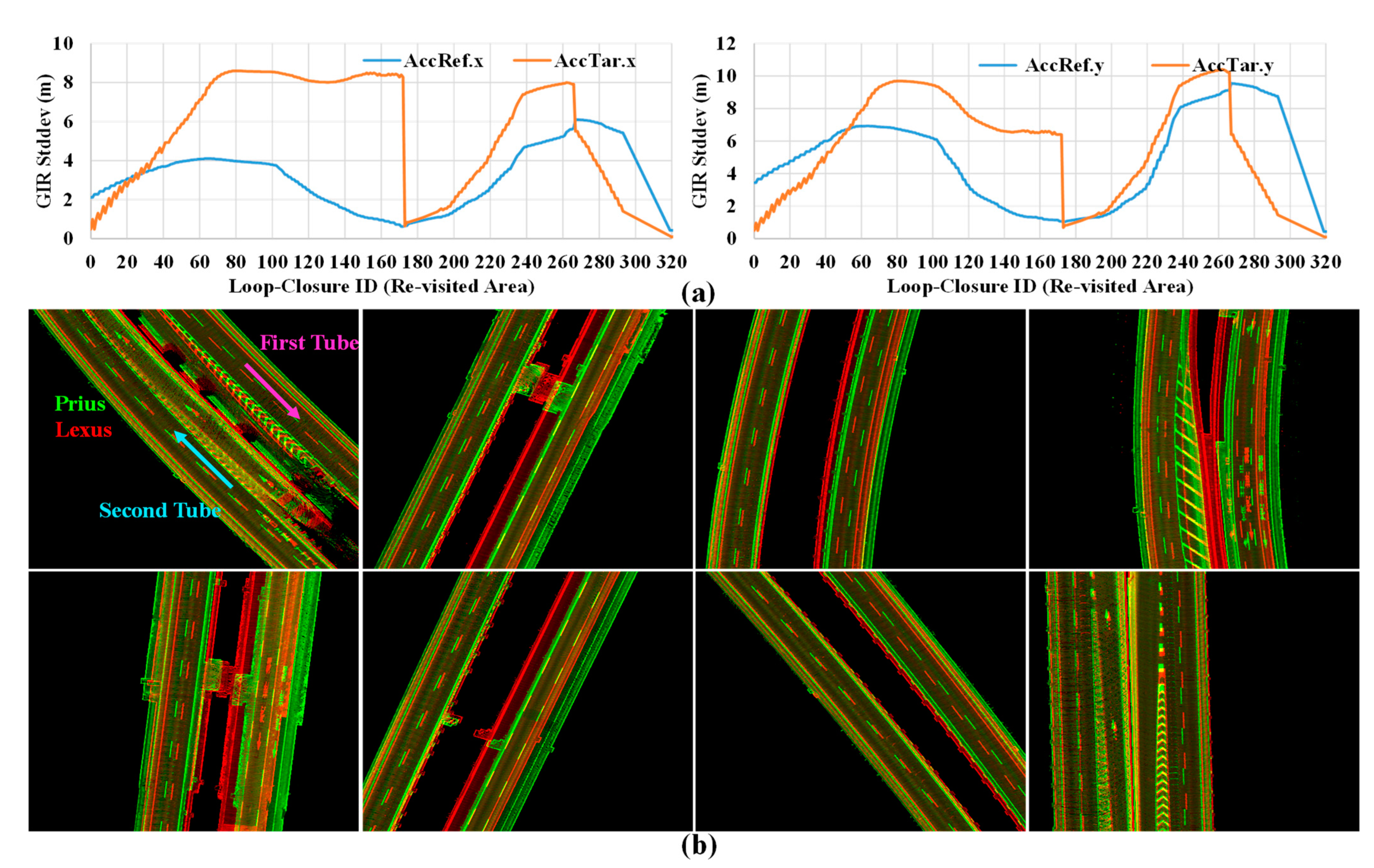
4.5. Mapping a Long Underground Tunnel Using Two Drives in the Same Driving Scenario and Tow Agents with Different Sensor Configurations

The capability to combine mapping data collected by different agents is very important to be integrated into the mapping modules. This paves the way to implement cloud source-based mapping systems and maintain the frequent updating process of the environment representation. However, a technical problem emerges in dealing with the different types of LIDARs due to the changes in the distribution pattern and the number of laser beams in the point clouds. This problem is settled down in the node strategy by using the 2D image domain to describe the road surfaces instead of the 3D point cloud domain. Another main issue is the use of different GIR systems and sensor configurations that affect the global accuracy of each agent. Therefore, the Yamate Tunnel (two tubes) was scanned by Lexus-1 (128 laser beams) in 2021 and combined with the map data of Prius (64 laser beams) in 2017. Figure 10a shows the corresponding GIR accuracy profiles in the two maps in the X and Y directions. The trajectory inside the tunnel is the same as in Figure 9a for the first tube for both agents; however, the driving scenario of the U-turn to visit the second tube was different. Thus, there were no loop closures between the two maps in the U-turn. This explains the reasons for the sudden change in the accuracy between the first and second tubes in Figure 10a. In addition, one can observe the considerable differences between the profiles to indicate that Prius’s map is more accurate than Lexus-1 in ACS. However, this indication is not necessarily true and relies on sensor configurations, i.e., Lexus-1′s GIR (PosLV 220) is more sophisticated than Pirus’s one (PosLV 110) in terms of manufacturing and sensor accuracy.
Figure 10b demonstrates many road patches in the combined GIR map with showing different patterns of distortions. Accordingly, the same analysis of the effects on the localization system in the previous chapter can be considered. This indicates that scanning such a challenging environment using GIR is not always accurate and merging multiple scans precisely is almost impossible. Moreover, it emphasizes the necessity to implement robust methods to improve the map accuracy because multiple scanning of such a highway environment is very necessary to increase the map density and quality due to the regulations of using high driving velocity.

4.6. Mapping a Critical Course Simultaneously Using Two following Agents with Same Sensor Configurations and Driving Scenarios

Lexus-1 and Lexus-2 were used to conduct this experiment, where they are identical in terms of sensor configurations and mass volume. An arterial course in Tokyo, starting from the waterfront area to the entrance of the Yamate Tunnel was scanned simultaneously. Lexus-1 exactly followed Lexus-2 by keeping a short distance to unify the driving scenario and the traffic flow. The course contains open-sky segments, underpasses covered by longitudinal bridges, short tunnels (2 km) and bridges surrounded by high buildings, as demonstrated in Figure 11a. As the vehicles were driven simultaneously, the loop closures between two scans continuously exist along the entire course and Figure 11b,c show the GIR accuracy profiles of the two agents in the X and Y directions, respectively. Surprisingly, the Lexus-2′s GIR system began to provide low accuracy of the position estimation in the underpass segment of the longitudinal bridge whereas this road structure did not affect the Lexus-1′s GIR system considerably. The low global accuracy of Lexus-2′s GIR gradually worsened all the way until reaching the entrance of the Yamate Tunnel. Accordingly, the GIR-combined map of these two simultaneous scans encodes environments at different global positions in ACS as demonstrated in Figure 11d. The images also show the scans of the environments in the opposite direction, where the deviations are less. This indicates that the GIR’s accuracy cannot be predicted and guaranteed in challenging environments even though using the same sensor configurations, driving scenarios and traffic flow.

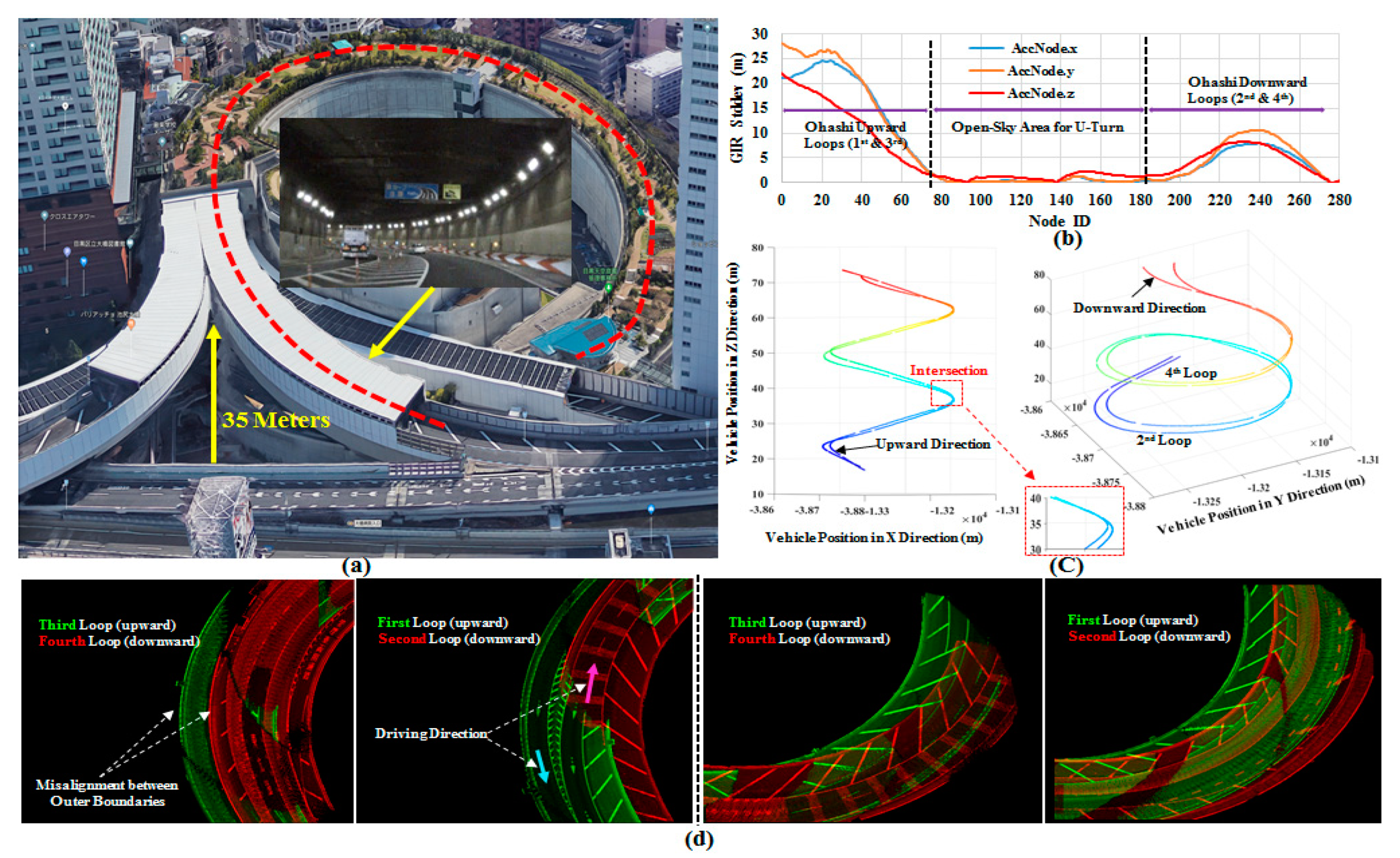
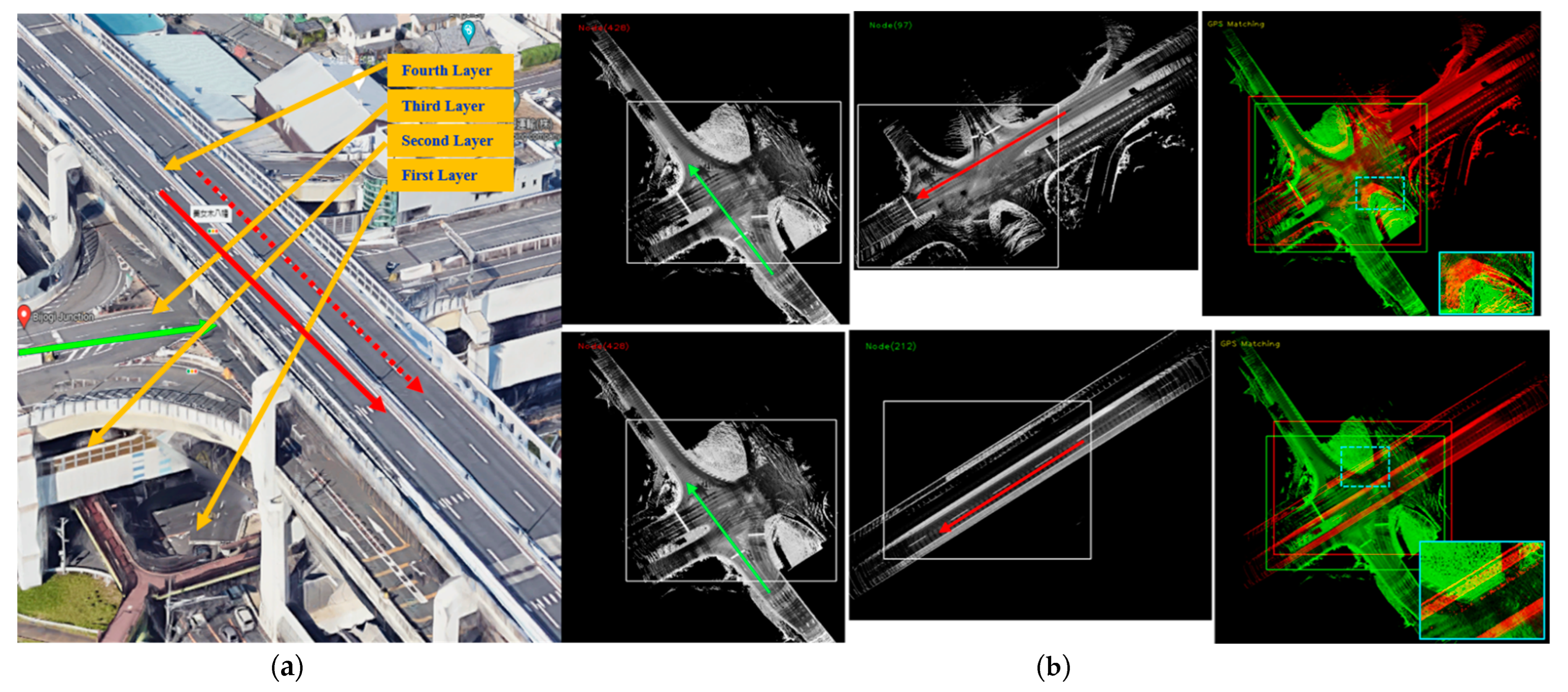
4.7. Mapping a Multilevel Environment Using Single Agent and Single Drive

Multilevel road structures are very critical to be mapped using GIR systems because of the obstruction of satellite signals by high layers. This affects the position estimation in both the XY and Z planes. In addition, the relative positions between layers must accurately be maintained to guarantee the true separation of the layers in the Z direction and the precise global consistency of the road structure in the XY direction. The GIR accuracy in the Z direction usually illustrates the same pattern and quality as those in the XY directions. Therefore, one can imagine the relevant effects of generating GIR elevation maps in the previous examples.
Ohashii Junction has been chosen to demonstrate the low capabilities of the GIR systems to accurately map multilevel environments. The junction is the terminal of the Yamate Tunnel and consists of four stacked loops ranging from 30 m underground to 35 m aboveground as demonstrated in Figure 12a. Two loops are connected to each tube of the Yamate Tunnel to allow driving in a single direction (upward or downward) and interfered with the other two loops in the Z direction, i.e., first and third loops are in the upward direction and linked with the first tube whereas the second and fourth loops are in the downward direction and connected to the second tube. Lexus-2 was used to encode the four loops starting from the deepest point at 30 m underground at the end of the Yamate Tunnel’s first tube to scan the upward two loops until the exit. The vehicle was then driven in an open-sky area to conduct a U-turn and visit the downward two loops.
Figure 12b shows the GIR accuracy profiles in Ohashi Junction in the X, Y and Z directions based on the coordinates of the nodes’ top-left corners, respectively. One can observe the massive change in the accuracy at the starting point because of driving inside the Yamate Tunnel. The accuracy has relatively been recovered in the open-sky road segment (U-turn) and distorted again when scanning the downward loops. This indicates the low quality of the GIR map in terms of accuracy and consistency in the XY and Z planes. Figure 12c illustrates the vehicle trajectory in Ohashi Junction by highlighting that the upward and downward loops have been intersected and represented in two elevation levels in ACS instead of four independent and interfered levels. Figure 12d illustrates this fact by showing four samples of the intersections between the first and second loops as well as the third and fourth loops in the same xy position. Therefore, each map image encodes the environments in two elevation levels in two opposite driving directions due to the huge elevation error, i.e., more than 10 m. Accordingly, the map in the upward direction will not be available during autonomous driving. Moreover, one can observe in Figure 12a that the loops have the same geometrical characteristics, especially in the exterior construction. On the other hand, the images in Figure 12d show the wrong consistency between loop boundaries due to the map errors in the XY plane. Consequently, this significantly affects the localization accuracy and makes conducting autonomous driving very risky using the GIR maps in the XY and Z planes.

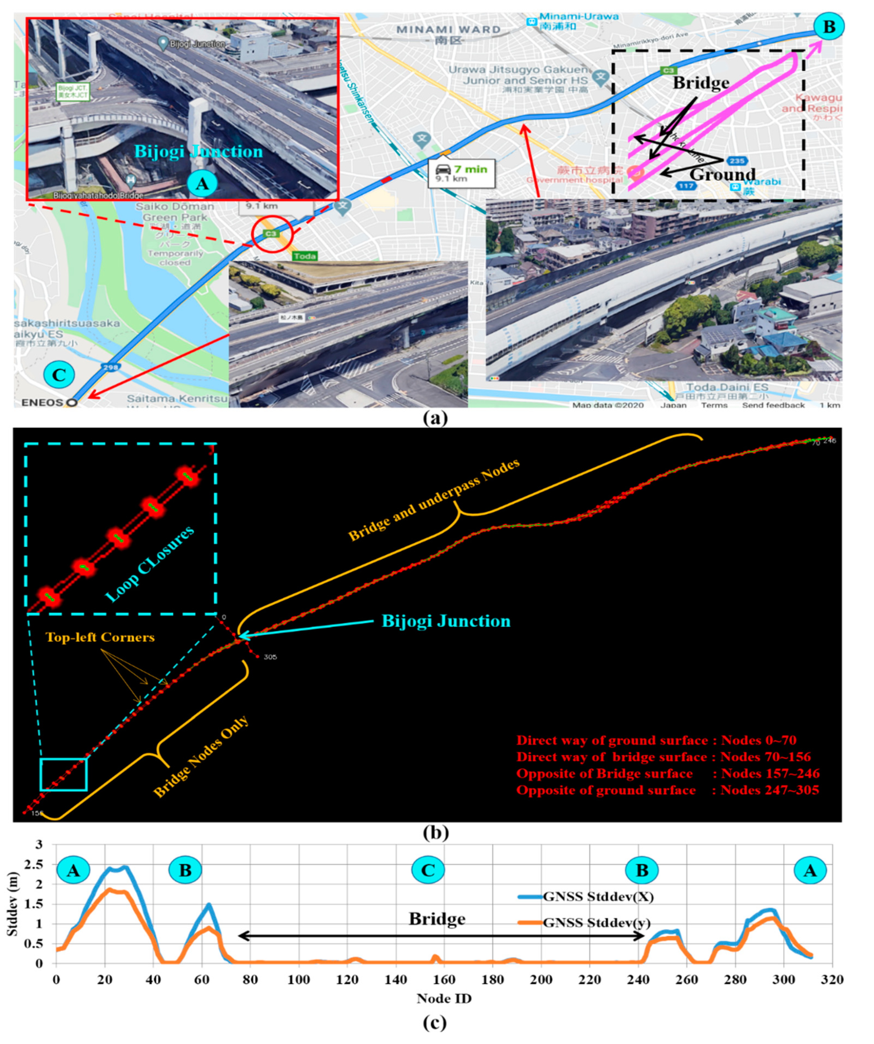
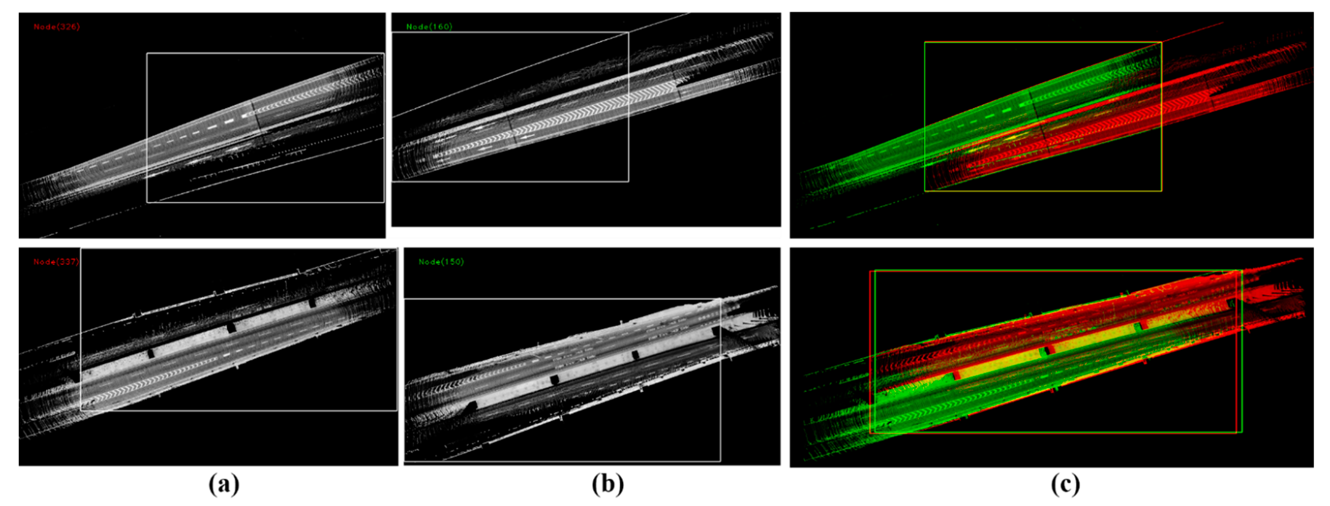
4.8. Mapping Longitudinal Bridge and Underpass Using Single Agent in Two Directions

Bijogi Junction in Tokyo represents a very challenging environment because the ground road surface (underpass) is covered by a longitudinal bridge for more than 15 km, as illustrated in Figure 13a. The driving scenario for collecting the map data started just before Bijogi Junction at point (A) to continuously scan the ground road surface until point (B). The direct lane in the bridge was then scanned until point (C), where the vehicle was U-turned to scan the bridge’s opposite lane towards point (B) again. The opposite lane of the underpass was then scanned until the corresponding road segment of point (A). The course covers around 40 km and is encoded by 305 nodes as demonstrated in Figure 13b. Accordingly, loop-closure events (289) continuously occurred because of scanning both bridge and ground layers in two directions.
Mapping longitudinal bridges and underpasses is a very crucial demand to enable the deployment of autonomous vehicles in modern cities. However, this demand is very difficult to be achieved using the GIR system due to the complexity of the road structures and the surrounding environments. Figure 13c shows the standard deviation profiles of the top-left corners in the X and Y directions that are obtained by the GIR system. It can be logically observed that the bridge nodes possess higher accuracy compared to the underpass road surface. This indicates the effects of the bridge obstructing the satellite signals. Figure 14 demonstrates this fact by showing two loop closures in the bridge and underpass layers, respectively. The GIR system particularly merges the bridge’s nodes of the direct and opposite lanes precisely because of the high signal quality whereas the underpass’s nodes demonstrate a massive longitudinal deviation.
Such multilevel environments require considering the consistency between layers to accurately share traffic information between vehicles during autonomous driving. Therefore, the global positioning accuracy of the layers should be evaluated in the road structure representation in the GIR maps. Figure 15a shows the Bijogi Junction at point (A) in Figure 13a consisting of four road levels in a plus structure shape. Figure 15b (first row) demonstrates the relative position error in the GIR map at the third layer by showing a lateral deviation between nodes created by different driving directions. In the second row, the GIR map demonstrated the inconsistency between the third and fourth layers by showing a massive misalignment of the road structure representation. This indicates the necessity to integrate SLAM technologies into the mapping modules in order to improve the map accuracy [19,26].

5. Conclusions

We proved that challenging environments such as dense trees, high buildings, long tunnels, multilevel structures and bridges are very critical in achieving precise mapping even when using expensive GNSS/INS-RTK systems. This is because of the high possibility of merging map data at revisited areas with different global positioning accuracies. This leads to deviations in positions, ghosting effects in landmarks, duplications in road surfaces and misalignments in multilevel structures. The main reasons for distortions are proved and concluded to be different driving scenarios, sensor configurations, map combinations and traffic flows. Consequently, GIR maps become very risky to be used during autonomous driving because they affect the localization accuracy for long distances. Furthermore, this paper emphasizes the necessity to integrate SLAM technologies into mapping modules in order to improve map accuracy. Otherwise, modern cities and many road segments will be excluded from autonomous vehicle deployment in the future. Moreover, the paper highlights many issues that are rarely discussed and investigated by researchers to be considered in the SLAM implementation phase such as the map combination/updating capability and the layer inconsistency in multilevel structures. Therefore, the challenging structures in this paper and the relevant analysis of the GIR map quality can be considered as baselines to create ideas and visions about the requirements of the mapping modules in the fourth and fifth levels of autonomous driving.

Author Contributions

M.A.: Investigation, Methodology, Resources, Software, Validation, Visualization, Writing—original draft, Writing—review, editing and Submission. N.S.: Supervision and Resources. R.Y.: Investigation, Data collection and Resources. K.Y.: Recourses and Admiration. All authors have read and agreed to the published version of the manuscript.

Funding

This work was partly supported by the Japan Society for the Promotion of Science (KAKENHI Funds: No. 20K19893 and No. 22K17974).

Conflicts of Interest

The authors declare no conflict of interest.

References

  1. Forster, C.; Pizzoli, M.; Scaramuzza, D. SVO: Fast semi-direct monocular visual odometry. In Proceedings of the 2014 IEEE International Conference on Robotics and Automation, ICRA 2014, Hong Kong, China, 31 May–7 June 2014; pp. 15–22. [Google Scholar]
  2. Rozenberszki, D.; Majdik, A.L. LOL: Lidar-only Odometry and Localization in 3D point cloud maps. In Proceedings of the 2020 IEEE International Conference on Robotics and Automation (ICRA), Paris, France, 31 May–21 August 2020; IEEE: Piscataway, NJ, USA, 2020; pp. 4379–4385. [Google Scholar]
  3. Lee, W.; Cho, H.; Hyeong, S.; Chung, W. Practical Modeling of GNSS for Autonomous Vehicles in Urban Environments. Sensors 2019, 19, 4236. [Google Scholar] [CrossRef] [PubMed]
  4. Kuramoto, A.; Aldibaja, M.A.; Yanase, R.; Kameyama, J.; Yoneda, K.; Suganuma, N. Mono-Camera based 3D Object Tracking Strategy for Autonomous Vehicles. In Proceedings of the IEEE Intelligent Vehicles Symposium (IV), Changshu, China, 26–30 June 2018; pp. 459–464. [Google Scholar] [CrossRef]
  5. Pendleton, S.D.; Andersen, H.; Du, X.; Shen, X.; Meghjani, M.; Eng, Y.H.; Rus, D.; Ang, M. Perception, Planning, Control, and Coordination for Autonomous Vehicles. Machines 2017, 5, 6. [Google Scholar] [CrossRef]
  6. Thrun, S.; Montemerlo, M. The Graph SLAM Algorithm with Applications to Large-Scale Mapping of Urban Structures. Int. J. Robot. Res. 2006, 25, 403–429. [Google Scholar] [CrossRef]
  7. Olson, E.; Agarwal, P. Inference on networks of mixtures for robust robot mapping. Int. J. Robot. Res. 2013, 32, 826–840. [Google Scholar] [CrossRef]
  8. Cadena, C.; Carlone, L.; Carrillo, H.; Latif, Y.; Scaramuzza, D.; Neira, J.; Reid, I.; Leonard, J.J. Past, Present, and Future of Simultaneous Localization and Mapping: Toward the Robust-Perception Age. IEEE Trans. Robot. 2016, 32, 1309–1332. [Google Scholar] [CrossRef]
  9. Roh, H.; Jeong, J.; Cho, Y.; Kim, A. Accurate Mobile Urban Mapping via Digital Map-Based SLAM †. Sensors 2016, 16, 1315. [Google Scholar] [CrossRef] [PubMed]
  10. Shan, T.; Englot, B. LeGO-LOAM: Lightweight and Ground-Optimized Lidar Odometry and Mapping on Variable Terrain. In Proceedings of the 2018 IEEE/RSJ International Conference on Intelligent Robots and Systems (IROS), Madrid, Spain, 1–5 October 2018. [Google Scholar] [CrossRef]
  11. Shan, T.; Englot, B.; Meyers, D.; Wang, W.; Ratti, C.; Rus, D. LIO-SAM: Tightly-coupled Lidar Inertial Odometry via Smoothing and Mapping. In Proceedings of the IEEE/RSJ International Conference on Intelligent Robots and Systems (IROS), Las Vegas, NV, USA, 24–30 October 2020; pp. 5135–5142. [Google Scholar]
  12. Yoon, J.; Kim, B. Vehicle Position Estimation Using Tire Model in Information Science and Applications; Springer: Berlin, Germany, 2015; Volume 339, pp. 761–768. [Google Scholar]
  13. Aldibaja, M.; Suganuma, N.; Yoneda, K. LIDAR-data accumulation strategy to generate high definition maps for autonomous vehicles. In Proceedings of the 2017 IEEE International Conference on Multisensor Fusion and Integration for Intelligent Systems (MFI), Daegu, Korea, 16–18 November 2017; pp. 422–428. [Google Scholar] [CrossRef]
  14. Aldibaja, M.; Suganuma, N.; Yoneda, K. Robust Intensity-Based Localization Method for Autonomous Driving on Snow–Wet Road Surface. IEEE Trans. Ind. Inform. 2017, 13, 2369–2378. [Google Scholar] [CrossRef]
  15. Aldibaja, M.; Yanase, R.; Kim, T.H.; Kuramoto, A.; Yoneda, K.; Suganuma, N. Accurate Elevation Maps based Graph-Slam Framework for Autonomous Driving. In Proceedings of the 2019 IEEE Intelligent Vehicles Symposium (IV), Paris, France, 9–12 June 2019; pp. 1254–1261. [Google Scholar] [CrossRef]
  16. Murakami, T.; Kitsukawa, Y.; Takeuchi, E.; Ninomiya, Y.; Meguro, J. Evaluation Technique of 3D Point Clouds for Autonomous Vehicles Using the Convergence of Matching Between the Points. In Proceedings of the 2020 IEEE/SICE International Symposium on System Integration (SII), Honolulu, HI, USA, 12–15 January 2020; pp. 722–725. [Google Scholar] [CrossRef]
  17. Qin, T.; Zheng, Y.; Chen, T.; Chen, Y.; Su, Q. RoadMap: A Light-Weight Semantic Map for Visual Localization towards Autonomous Driving. In Proceedings of the 2021 IEEE International Conference on Robotics and Automation (ICRA), Xi’an, China, 30 May–5 June 2021. [Google Scholar]
  18. Ahmad, F.; Qiu, H.; Eells, R.; Bai, F.; Govindan, R. CarMap: Fast 3D Feature Map Updates for Automobiles; 2020. Available online: https://www.usenix.org/conference/nsdi20/presentation/ahmad (accessed on 30 May 2022).
  19. Aldibaja, M.; Suganuma, N. Graph SLAM-Based 2.5D LIDAR Mapping Module for Autonomous Vehicles. Remote Sens. 2021, 13, 5066. [Google Scholar] [CrossRef]
  20. Nam, T.H.; Shim, J.H.; Cho, Y.I. A 2.5D Map-Based Mobile Robot Localization via Cooperation of Aerial and Ground Robots. Sensors 2017, 17, 2730. [Google Scholar] [CrossRef] [PubMed]
  21. Sun, L.; Zhao, J.; He, X.; Ye, C. DLO: Direct LiDAR Odometry for 2.5D Outdoor Environment. In Proceedings of the 2018 IEEE Intelligent Vehicles Symposium (IV), Changshu, China, 26–30 June 2018; pp. 1–5. [Google Scholar]
  22. Eising, C.; Pereira, L.; Horgan, J.; Selvaraju, A.; McDonald, J.; Moran, P. 2.5D vehicle odometry estimation. IET Intell. Transp. Syst. 2021, 16, 292–308. [Google Scholar] [CrossRef]
  23. Available online: https://www.applanix.com/pdf/faq_pos_av_rev_2a.pdf (accessed on 30 May 2022).
  24. Available online: https://www.applanix.com/pdf/PosPac%20MMS_LAND_Brochure.pdf (accessed on 30 May 2022).
  25. Aldibaja, M.; Suganuma, N.; Yanase, R.; Cao, L.; Yoneda, K.; Kuramoto, A. Loop-Closure and Map-Combiner Detection Strategy based on LIDAR Reflectance and Elevation Maps. In Proceedings of the 2020 IEEE 23rd International Conference on Intelligent Transportation Systems (ITSC), Rhodes, Greece, 20–23 September 2020; pp. 1–7. [Google Scholar] [CrossRef]
  26. Triebel, R.; Pfaff, P.; Burgard, W. Multi-Level Surface Maps for Outdoor Terrain Mapping and Loop Closing. In Proceedings of the 2006 IEEE/RSJ International Conference on Intelligent Robots and Systems, Beijing, China, 9–15 October 2006; pp. 2276–2282. [Google Scholar] [CrossRef]
Figure 1. Node strategy. (a) Intensity image to represent the road surface by accumulating LIDAR frames according to the vehicle trajectory. Top-left corner is the identification of the node in the XY plane and determined by the maximum vehicle position in the driving area with respect to ACS. (b) Elevation image to express the height of each pixel in the road surface and identified in ACS by the average value.
Remotesensing 14 04058 g001
Figure 2. Challenging environments to be mapped by GIR. Dense trees, high buildings, long tunnels, covered roads by railway bridges, longitudinal tunnels and multilevel road structures.
Remotesensing 14 04058 g002
Figure 3. Different patterns of ghosting and duplications in distorting the road surface by GIR systems.
Remotesensing 14 04058 g003
Figure 4. Experimental platforms with different sensor configurations. Prius with LIDAR HDL-64 S2 and Applanix PosLV 110 GIR, Alphard with LIDAR 64 and PosLV 220 and two identical Lexus cars with LIDAR VLS-128-AP and PosLV 220.
Remotesensing 14 04058 g004
Figure 5. Driving under the bridge in two directions with surrounding high buildings. (a) The vehicle trajectory is represented by nodes with indicating loop closures by green links. (b) Accuracy profiles of the GIR system along the revisited areas (in two opposite lanes) in X and Y directions. (c) Different ghosting patterns in GIR map in lateral and longitudinal directions by flipping the road lanes at the most correct image.
Remotesensing 14 04058 g005
Figure 6. Mapping Tokyo’s waterfront with high buildings, dense trees and railways using two collection phases. (a) The vehicle trajectories in the two phases highlight critical road segments. (b,c) The node distribution in each phase with the local loop closures by green links. (d) Map combination links between two phases.
Remotesensing 14 04058 g006
Figure 7. Ghosting (indicated by ellipses) in GIR map of the three segments in Figure 6a. (a,b) Representation of local loop closures in the first collection phase in opposite directions. (c) GIR map images with ghosting effects and deviations in landmarks. (d) Single scans by the second collection phase. (e,f) Map combination: individual merging of images in (d) with (a,b), respectively.
Remotesensing 14 04058 g007
Figure 8. Final representations of road segments in Figure 6 and Figure 7 in the GIR combined map with highlighted distorted areas in red ellipses and lines.
Remotesensing 14 04058 g008
Figure 9. Scanning the world’s longest tunnel two times by the same agent. (a) Nodes along the course with showing identical distribution in two scans. (b,c) GIR accuracy profile in XY directions indicating high accuracy in the open-sky area because of receiving good quality satellite signals and low accuracy all the way inside the tunnel. (d) Road surface images in the first scan. (e) GIR-combined map images showing the massive deviation between two scans.
Remotesensing 14 04058 g009
Figure 10. Scanning two tubes of the world’s longest tunnel using two agents with different sensor configurations. (a) GIR accuracy of each agent in X and Y directions. (b) GIR combined map images showing different deviations in lateral and longitudinal directions along the first and second tubes.
Remotesensing 14 04058 g010
Figure 11. Mapping a critical environment simultaneously using two agents with the same driving scenario and sensor configuration. (a) Driving scenario by nodes from Odaiba area to the entrance of the Yamate Tunnel. (b,c) GIR accuracy in X and Y directions of the two agents. (d) GIR combined map.
Remotesensing 14 04058 g011
Figure 12. Mapping multilevel Ohashi Junction in Tokyo. (a) Rood structure ranging from 30 m underground to 35 m aboveground using four loops. (b) GIR accuracy in X, Y and Z directions indicating a big difference between upward and downward loops. (c) Upward loops have been intersected with downward loops by GIR instead to be interfered with around 10 m relative positions in the Z direction (the change of color demonstrates the change of height). (d) GIR map images in the same xy coordinates in each pair showing the intersections between layers representing road surfaces in opposite directions at the same elevation level.
Remotesensing 14 04058 g012
Figure 13. Mapping multilevel Bijogi Junction with longitudinal bridge and underpass. (a) The course representation showing continuous covering of the underpass by the wide bridge shoulders. (b) Nodes’ top-left corner distributed in ACS based on GIR coordinates with indicating the continuous loop closures in each layer because of scanning direct and opposite lanes. (c) GIR standard deviation of the top-left corners in x and y directions indicating the high quality of satellite signals of bridge’s nodes and considerable low accuracy in the underpass’s nodes.
Remotesensing 14 04058 g013
Figure 14. GIR map accuracy in the same global area in XY plane in the two layers of the bridge (1st row) and underpass (2nd row). (a) Node of the direct lane. (b) Node of the opposite lane. (c) Merging two nodes using the GIR system. The underpass layer shows a massive longitudinal deviation because of the obstruction of satellite signals by the bridge layer.
Remotesensing 14 04058 g014
Figure 15. GIR map inconsistency at Bijogi Junction in the same global area in XY plane. (a) Road structure in Bijogi Junction consisting of four layers of a plus shape. (b) First row: relative position error between two nodes at the third layer that were scanned in different driving directions. Second row: GIR map inconsistency between third and fourth layers at the same global area in the XY plane showing the misalignment of the road structure.
Remotesensing 14 04058 g015
Publisher’s Note: MDPI stays neutral with regard to jurisdictional claims in published maps and institutional affiliations.

