Article

2.5D Layered Sub-Image LIDAR Maps for Autonomous Driving in Multilevel Environments

The Advanced Mobility Research Institute, Kanazawa University, Kanazawa 920-1192, Japan
*
Author to whom correspondence should be addressed.
Remote Sens. 2022, 14(22), 5847; https://doi.org/10.3390/rs14225847
Submission received: 13 October 2022 / Revised: 17 November 2022 / Accepted: 17 November 2022 / Published: 18 November 2022

Abstract

:
This paper proposes a reliable framework to map multilevel road structures in the 2D image domain called layered sub-image maps (LSM). The road is divided into a set of sub-areas providing IDs in the XY plane. Each sub-area is decomposed into several layered images using LIDAR intensity and elevation data to form a 2.5D map image. The layered elevation images are given IDs in the Z plane to represent the height of the contained road features in meter-order whereas the elevation pixels indicate the cm-order of the road slope in the range of 200 cm. The layered intensity images are then created to describe the road surface in conjunction with the number of the layered elevation images and the corresponding pixel distributions. A significant map retrieval strategy during autonomous driving has been designed based on the LSM implementation tactic and the IDs in the XYZ plane. The system’s reliability has been proved by a unique localization module to localize an autonomous vehicle in a challenging multilevel environment consisting of four stacked loops with an average accuracy of 5 cm in lateral, longitudinal and altitudinal directions.

Graphical Abstract

1. Introduction

Mapping in multilevel environments is a challenging and important requirement to deploy autonomous vehicles in modern cities that are packed with longitudinal bridges and underground tunnels. The mapping tactic in such environments including map creation, places identification in the absolute coordinate system (ACS) and storing strategy plays the main role in designing the localization module. This is because the maps should be completely retrieved for each layer based on the vehicle position in the XYZ plane during autonomous driving. The matching process between the map and sensory data can be then conducted safely to correct the localization errors [1,2,3,4]. Therefore, mapping and localization in multilayer road structures are considered as a challenging demand in levels four and five of autonomous driving and are rarely discussed in the autonomous vehicle research field.
Triebel has proposed a method called a multi-level surface map (MLS) to classify environment patches into traversable, non-traversable and vertical [5]. The idea is to divide environments into cells that can encode many surfaces based on the mean and the variance of the height as well as the depth of the vertical extension [6]. This facilitates distinguishing the bridge and underpass patches in a local LIDAR point cloud. In addition, it significantly enhances the matching result by iterative closest point (ICP) to correct the relative-positions errors of scanning the same places and creates maps using SLAM technologies [7,8]. The generated maps have been used for enabling path planning and localization in [9] with reliable results of surfing in a ground parking lot. Kummerle has used MLS maps to scan a multilayer parking lot and conduct autonomous localization accordingly [10]. However, storing depth, height and variance of cells (20 cm) in each point cloud is a high-cost process and occupies a large size of memory to create large maps. In addition, it increases the processing time to retrieve maps during autonomous driving because of the need to add an ID to each cell. Furthermore, MLS has been designed to operate in the 3D point cloud domain to provide the shape and distribution patterns of the classified features. Consequently, the MLS maps are very applicable in small areas because the size of cells should be preserved small to ensure sufficient resolution of the environment representation. Accordingly, we extend our previous work [11] and propose a reliable strategy to map multilevel environments in the 2D image domain and represent the intensity and elevation of road surfaces, i.e., layered sub-image maps (LSM). In addition, a 3D localization module is explained to significantly utilize LSMs to estimate the xyz vehicle position during autonomous driving. A complex highway multilayer road junction in Tokyo was used to emphasize the robustness, scalability and efficiency of the proposed system to safely retrieve maps in layers and localize vehicles accordingly.

2. Previous Work

In the previous work [11], we proposed a 2D mapping strategy of road surfaces while considering the point cloud accumulation, the storing size of map images and the identification of the images in an ACS. To address these issues, the dynamic objects in the LIDAR point clouds are filtered out based on the velocity (more than 0.4 km/h) and a height threshold. The height threshold is set to 0.3 m to preserve the points of stationary environmental features such as painted landmarks and curbs as well as the lower parts of trees, road edges, barriers, poles, traffic lights and so on. A 2D LIDAR intensity frame is then generated by converting the filtered point cloud into an image based on the laser beam reflectivity as shown in Figure 1a. This is achieved using a series of transformations between an ACS, a vehicle, LIDAR and image coordinate systems. The LIDAR frames are then accumulated in an intensity image based on the vehicle trajectory as illustrated in Figure 1b–d. The accumulation process is terminated by exceeding the number of pixels of a fixed threshold λ as demonstrated in Figure 1e and a node is produced accordingly. The top-left corner CTF is used to identify the node in the ACS and the coordinates are determined by the maximum xy vehicle positions inside the driving area as indicated in Figure 1e. The node’s intensity image is then divided into a set of sub-images with fixed width and height s w × s h . The top-left corner is utilized to label the sub-images by global IDs (x, y) as in Equation (1) and Figure 1f. The IDs are used to save the sub-images into a hard disc in a BMP image compression format. These technical steps are continuously applied to create new nodes and extend the map size in the image domain.
I D ( x ) = f l o o r ( C T F ( x ) / S W )   I D ( y ) = c e i l     ( C T F ( y ) / S h )  

3. Problem Statement

The mapping system in [11] has been used to generate maps for more than 7000 km in different cities in Japan. A GNSS/INS-RTK (GIR) system has been used to estimate the vehicle position during the data collection phase and calculate the node top-left corners’ xy coordinates in the ACS. Accordingly, the intensity maps are generated and stored by sub-images with the corresponding XY-IDs. A robust localization system has been proposed to localize the vehicle using the intensity maps in the XY plane [12]. The need to perform autonomous driving in multilayer road structures has then emerged and the problem of encoding different layers in the same 2D sub-image has been observed [13,14]. Accordingly, considerable localization errors may occur in the overlapped zones such as bridges, tunnels and multi-level parking lots because they share the same IDs (x, y). Figure 2a shows an environment of three road layers, i.e., a ground tunnel, a bridge tunnel and a mountain road. The overlapping of these layers in the 2D sub-image completely distorts the road structure representation as illustrated in Figure 2b. Consequently, the localization module fails to estimate the vehicle position because the sensory data (observation image) encode only the road surface of a unique layer during autonomous driving. Figure 2c–e shows that the map image is overlapped by the observation image in each layer based on the matching score. The red and yellow circles imply the actual and estimated vehicle positions, respectively. The red rectangle demonstrates the correct overlapping of the observation image based on the actual position. A lateral deviation occurs in the ground-tunnel layer, i.e., the middle-dashed lines do not match those in the map image. A longitudinal deviation is produced in the bridge-tunnel layer that indicates the road context is not aligned properly. Finally, a perfect match is obtained in the mountain layer because of the unique road pattern compared to the parallel patterns of the other two layers. Therefore, the road layers must automatically be distinguished and registered in the maps and the localization system must be modified to estimate the vehicle position in the XYZ plane, accordingly.

4. Proposed Solution

4.1. Mapping Multilayer road Structures

The above problem can be solved by separating the road layers in the map images based on the altitudinal values in the ACS. We modified the mapping system to generate maps in two representations: intensity and elevation, i.e., 2.5D maps [15,16,17]. The intensity image describes the road surface in grayscale pixels whereas the elevation image encodes the height value of each pixel in the real world. Therefore, the same technical steps in Section 2 are simultaneously applied to produce the elevation images of the nodes in a float format as particularly detailed below.
Given a rotation matrix R by the IMU system at a vehicle position p, the index (u, v) of a pixel can be calculated using Equations (2)–(4) with respect to the pixel resolution σ.
p = [ p x ' p y ' p z ' ] = R P
u = S w 2 + p x ' σ
v = S h 2 + p y ' σ
The corresponding height of p in the is obtained by adding the vehicle z position as in Equation (5).
z u , v = p z ' + z t v
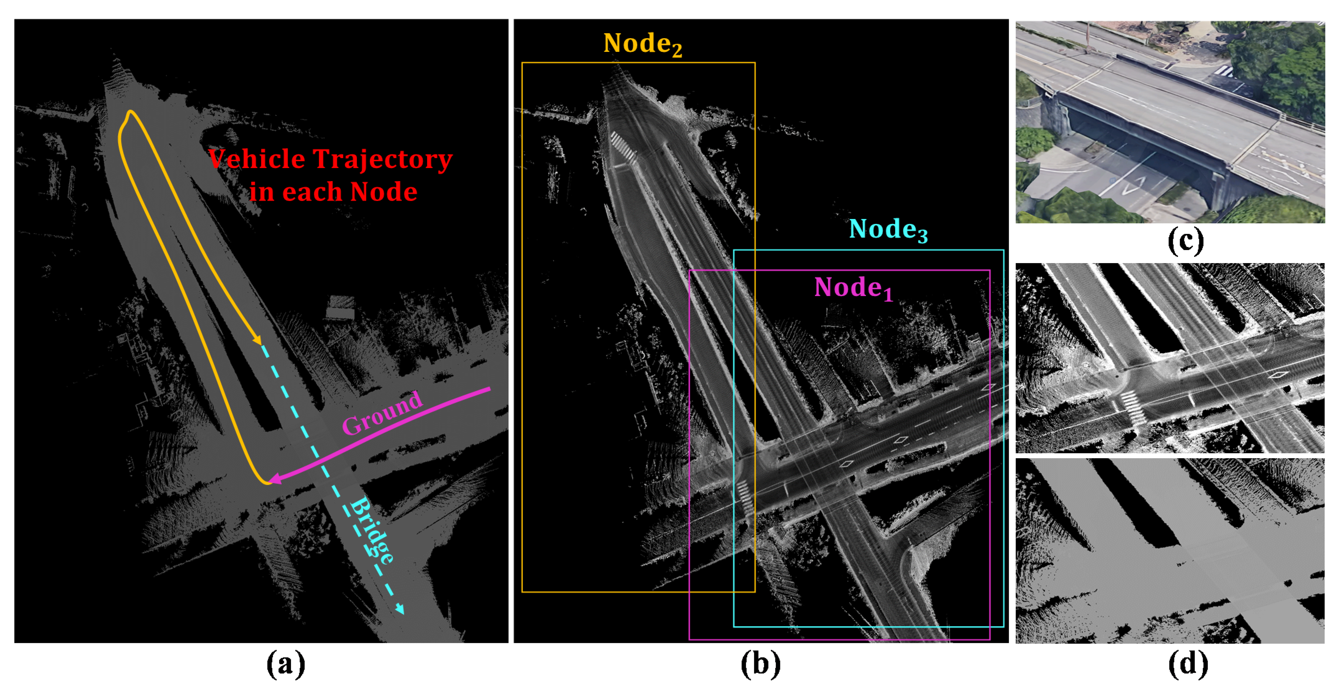
Thus, the LIDAR elevation frame is formed at each vehicle position and accumulated in an elevation map image as demonstrated for a bridge-underpass environment in Figure 3a. The environment is encoded by three nodes based on λ and merged in the ACS using the top-left corner’s coordinates in Figure 3b. The common area between the bridge and underpass occurs in the first and third nodes as demonstrated in Figure 3c. The underpass is first saved in the sub-images of the first node with the IDs (x, y). Based on the vehicle trajectory in Figure 3a, the bridge segment in the third node is used to update the saved sub-images of the first nodes because they share the same IDs (x, y), i.e., loop closure events [18]. Accordingly, the two layers are encoded in the same sub-image and distort the road representation in the XY and Z planes as illustrated in Figure 3d. In order to solve this problem, we considered the identification of sub-images in the Z plane by providing IDs (z) and mapping the road layers individually.
Storing elevation maps is very tricky and critical because of the need to include float values. In addition, an elevation map image may contain a particular set of pixels that demonstrate a considerable change in the height values because of the road slope. Therefore, identifying the road layers by IDs (z) must be addressed properly.
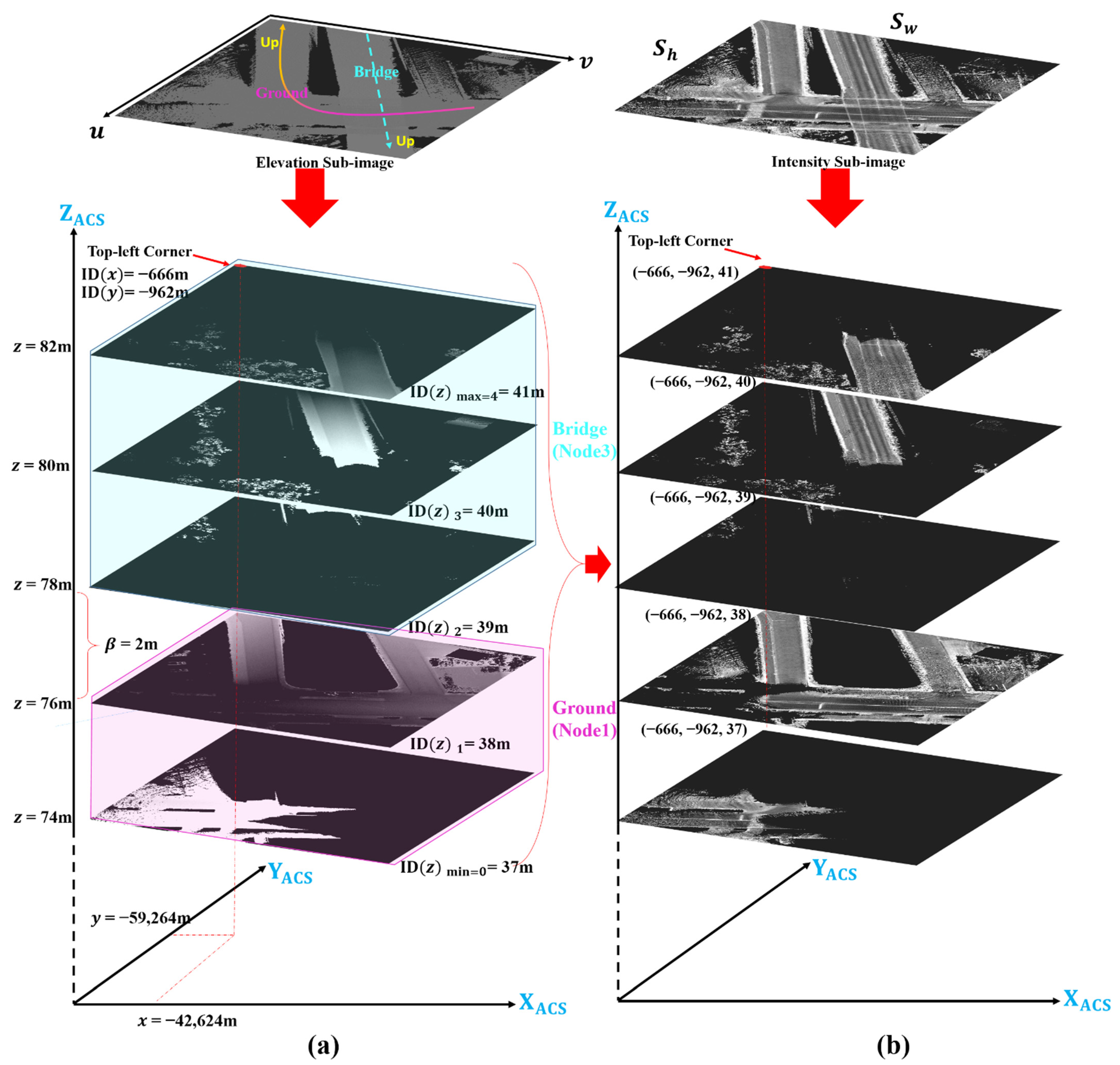
The ACS is virtually sampled into layers according to an altitudinal threshold β. The threshold is selected to be less than the standard norm distance between bridge and ground road surfaces, e.g., 2 m. Based on β, each layer can be given an ID (z) to represent the altitudinal range in the meter order. The height of the environmental features in each layer is then encoded by an elevation image in the cm-order with respect to the given ID (z) and the road slope. Finally, the pixels of the road surface are integrated and distributed in a set of layered intensity images according to the feature existence in the layered elevation images.
The simplest strategy to achieve the above tactic is to apply the above steps to each sub-image and create the LSM. The sub-image of the common area in the first node is initially considered. The maximum and minimum altitudinal values   Z m a x and   Z m i n are calculated and the corresponding two boundary layers in ACS are determined using Equation (6).
I D ( z ) m a x = f l o o r ( z m a x / β )   I D ( z ) m i n = f l o o r ( z m i n / β )  
Based on the two boundary layers and β, the in-between layers are simply initialized with the corresponding IDs (z) as demonstrated in Figure 4a in the pink polygon. A layer’s plane ith can mathematically be represented by Equation (7) according to the normal vector [ n x ,   n y ,   n z ] T = [ 0 , 0 , 1 ] T .
n x ( x x t v ) + n y ( y y t v ) + n z ( z I D ( z ) t ) = 0
where [ x ,   y ,   z ] T is an arbitrary position in the plane with the altitudinal range of IDs (z)i + β. Hence, the pixels in the layered elevation sub-image are classified and distributed on the created planes and the coordinates of a feature in an ith layer are restored in the ACS using Equation (8).
x = ( S w σ I D ( x ) ) + σ u y = ( S h σ I D ( y ) ) + σ v   z = ( 255 γ I D ( z ) ) + γ w
The corresponding intensity sub-image of the road surface is decomposed into the same number of layers as demonstrated in Figure 4b. The road surface pixels are then assigned according to the distribution in each elevation layer. The layered elevation and intensity images are saved with the IDs (x, y, z). These IDs are effectively utilized to update the saved images and automatically add new layers to encode different levels of the same road structures, e.g., the bridge segment is added after creating the third node and represented by three planes as surrounded by the cyan polygon.

4.2. Multilayer Map Retrievel during Autonomous Driving

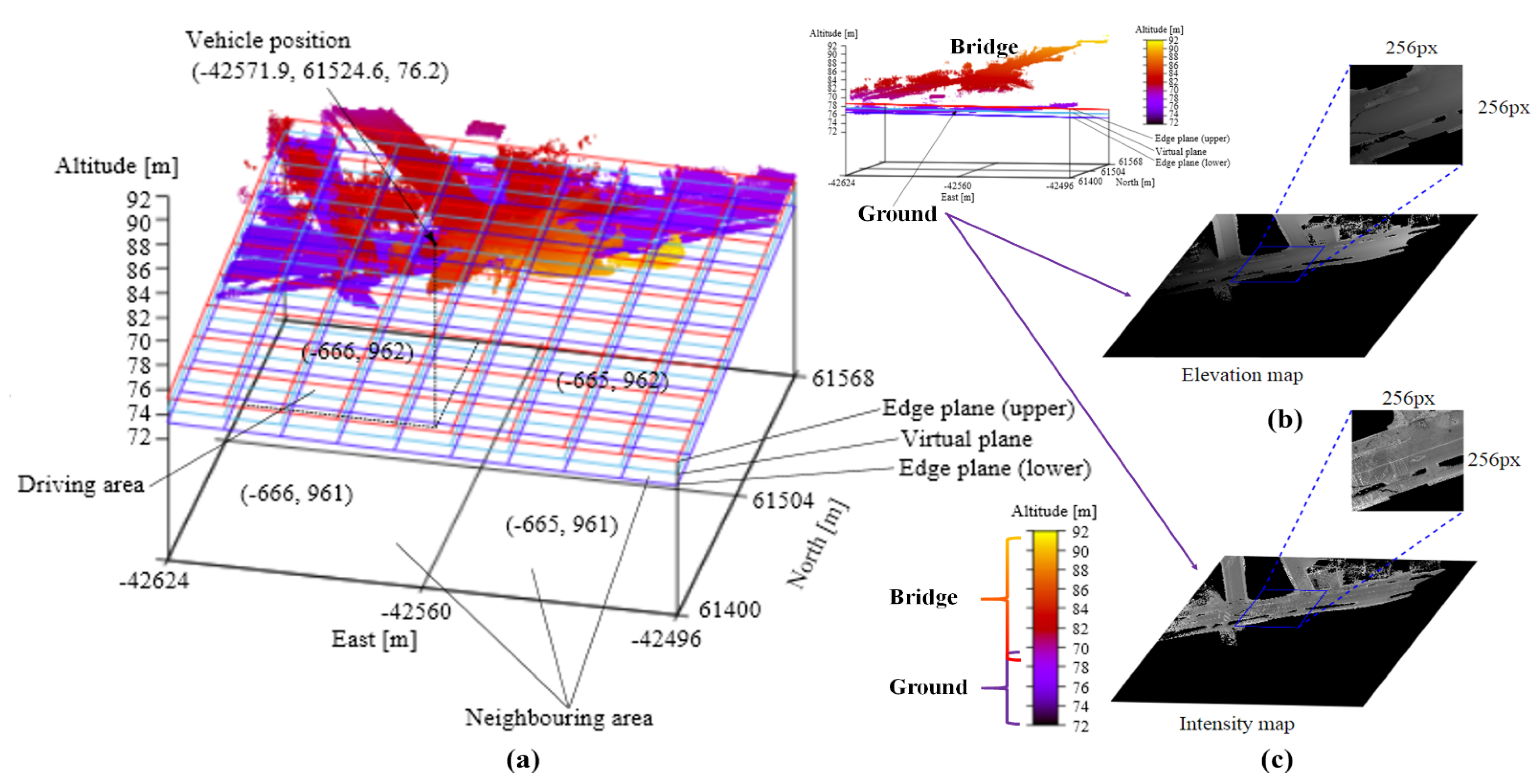
Retrieving map during autonomous driving is a difficult issue because it needs to be strategized according to the localization system. Given a vehicle pose, the ID (x, y) of the driving area in the ACS can be obtained by Equation (1) as illustrated in Figure 5a, i.e., CTF is replaced with the vehicle pose’s xy coordinates. The three neighboring areas are identified by frequently adding one unit to the driving area ID (x, y). The four areas create a virtual plane that is rotated based on the pitch and roll angles Rot and elevated by the z vehicle position. The plane is represented by the normal vector [ n x ,   n y ,   n z ] T = R o t [ 0 , 0 , 1 ] T . Another two edge planes (lower and upper) passing through the points of ( x t v + n 2 n x , y t v + n 2 n y , z t v + n 2 n z ) and   ( x t v + n 2 n x , y t v + n 2 n y , z t v n 2 n z ) are assumed to determine the altitudinal range of each pixel in the plane. Accordingly, the layered elevation sub-images in the four areas are restored based on the IDs (z) in the altitudinal range. The pixels in the virtual plane are then assigned by averaging the elevation values between the edge planes as shown in Figure 5b. The resultant plane is called the large elevation map image. This image is cut off around the vehicle with a fixed size to create the elevation map image that will be used to localize the vehicle in the Z direction. Based on the pixel distribution in the elevation map image and IDs (z), the corresponding pixels in the layered intensity sub-images are averaged to form the intensity map image and express the road surface as demonstrated in Figure 5c. Likewise, the image is cut off to obtain the intensity map image that will be used to localize the vehicle in the XY plane.

5. LSM Based Localization in Multilevel Environments

The localization system is a critical pillar to enable autonomous driving. The vehicle must be localized in the longitudinal direction with respect to the road context, in the lateral direction with respect to the lane lines and in the altitudinal direction with respect to the road structure [19,20,21]. As safety is a prime priority, dead reckoning (DR) is employed to estimate the vehicle position   X t , DR   using on-board sensors [22,23]. This is achieved by integrating the time interval Δt and the vehicle velocity v to the previous position   X t 1 , DR as clarified in Equation (9).
X t , DR = X t 1 , DR + v t Δ t
The DR accuracy is inversely proportional to the distance from the initial position. Therefore, the accuracy is recovered to precisely estimate the vehicle position   X t , ACS   by a translation offset   Δ X t . ACS , DR   in Equation (10) based on matching the elevation-intensity map images and the online LIDAR point clouds as detailed in the next section.
X t , ACS = X t . ACS , DR + Δ X t . ACS , DR

5.1. Localization in XY Plane

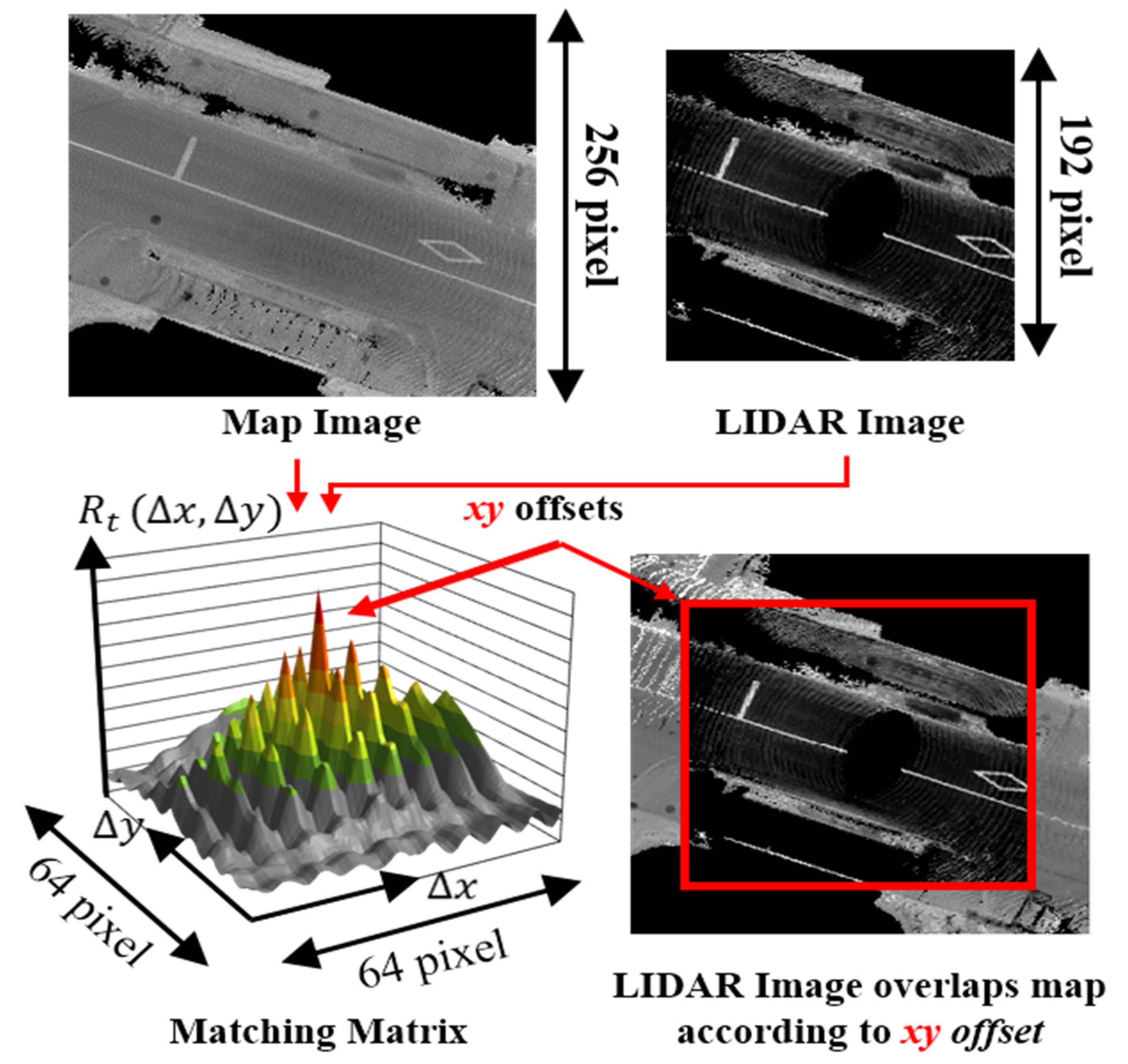
The DR estimation is used to retrieve the LSM as explained in Section 4.2. The LIDAR encodes the surrounding environment according to the actual position of the vehicle in the real world. The LIDAR point clouds are down-sampled and converted into an intensity image to describe the road surface on the grayscale level. The intensity image is utilized to calculate the similarity score R ( Δ x , Δ y )   with the intensity map image using zero normalized cross correlation (ZNCC) as mathematically explained in (11) and demonstrated in Figure 6.
R ( Δ x , Δ y ) = i = 0 N 1 { ( Δ x , Δ y ) m ¯ } { z i z ¯ } i = 0 N 1 { m i ( Δ x , Δ y ) m ¯ } 2 i = 0 N 1 { z i z ¯ } 2
This equation provides a matching matrix to indicate the location of the LIDAR image in the map image by the highest peak. As localization is not a deterministic process, the estimations must be tracked in a probabilistic framework. Therefore, the matching matrix is multiplied by the prior probability P t ¯ ( Δ x , Δ y ) to obtain the posterior probability   P t as clarified in Equation (12).
P t ( Δ x , Δ y ) = η ( R t ( Δ x , Δ y ) + 1 ) P t ¯ ( Δ x , Δ y )
The offsets   X t . ACS , DR   are then calculated based on the posterior probability and the corrected vehicle position is obtained accordingly, using Equation (10).

5.2. Localization in Z Plane

Based on   Δ X t . ACS , DR   the retrieved MLS is cut off to be in the same size (width and height) of the LIDAR frame as shown in Figure 7. The LIDAR point cloud is converted into an elevation image in the same manner that is mentioned in Section 4.1. A histogram on the altitudinal differences between the pixels in the LIDAR and map elevation images is formed. The histogram is converted into a probability distribution vector   P t o b s   by normalizing the bars based on the Otsu threshold lt [24] and scaling up by the Sigmoid function as implied in Equation (13).
P t o b s ( Δ z ) = ( 1 + e α ( l l t ) ) 1
A binary Bayes filter (BBF) is then incorporated to model the distribution variance with respect to the time [25] and calculate the altitudinal posterior probability as in Equation (10).
P t ( Δ z ) = ( 1 + e L t ) 1 ,   L t = log ( P t o b s / 1 P t o b s ) + log ( P t 1 o b s / 1 P t 1 o b s )
where   P t   is the posterior probability and   P t 1   is the prior probability. The position of the highest peak in the vector refers to the altitudinal offset that should be added to correct DR measurements and obtain the z vehicle position.

6. Experimental Results and Discussion

6.1. Setup Configuration

Figure 8 shows the experimental platform equipped with many sensors to enable autonomous driving. A Velodyne HDL-64E S2 with 64 laser beams is attached to the roof to scan the surrounding environments and generate 3D point clouds. Two GNSS antennas are also attached and connected to an Applanix POS-LV 220 (GIR) coupled GNSS/IMU system to record various measurements such as velocity and pose. These data are post-processed to produce a highly accurate vehicle trajectory in the ACS and the mapping module is then activated to generate elevation and intensity maps.
During autonomous driving, the DR technique was employed to estimate the 3D vehicle position using the maps and the proposed localization modules in the XY and Z directions. In order to evaluate the system’s performance, the Applanix system was also activated to generate the ground truth. The central processing unit was deployed in the trunk and possesses Intel-Core™ i7-6700 CPU working at 3.40 GHz with 8 GB RAM. The operating system is Windows-7 64X and the localization and mapping systems were coded in VS-2010 C++ using OpenCV and OpenGL libraries.
The parameters of the LSM and localization systems are set as follows: λ = 10242 is the pixel number to create a node, the pixel resolution σ is 12.5 cm in the real world and β = 2 m is the altitudinal threshold to divide ACS into layers. The size of a layer map sub-image is Sw × Sh = 512 × 512. In the localization module, the dimensions of the large map image is 2Sw × 2Sh and the LIDAR image is in the size of 192 × 192. The maximum velocity during autonomous driving is set to 60 km/h.

6.2. Analysing the Mapping System in Ohashi Junction

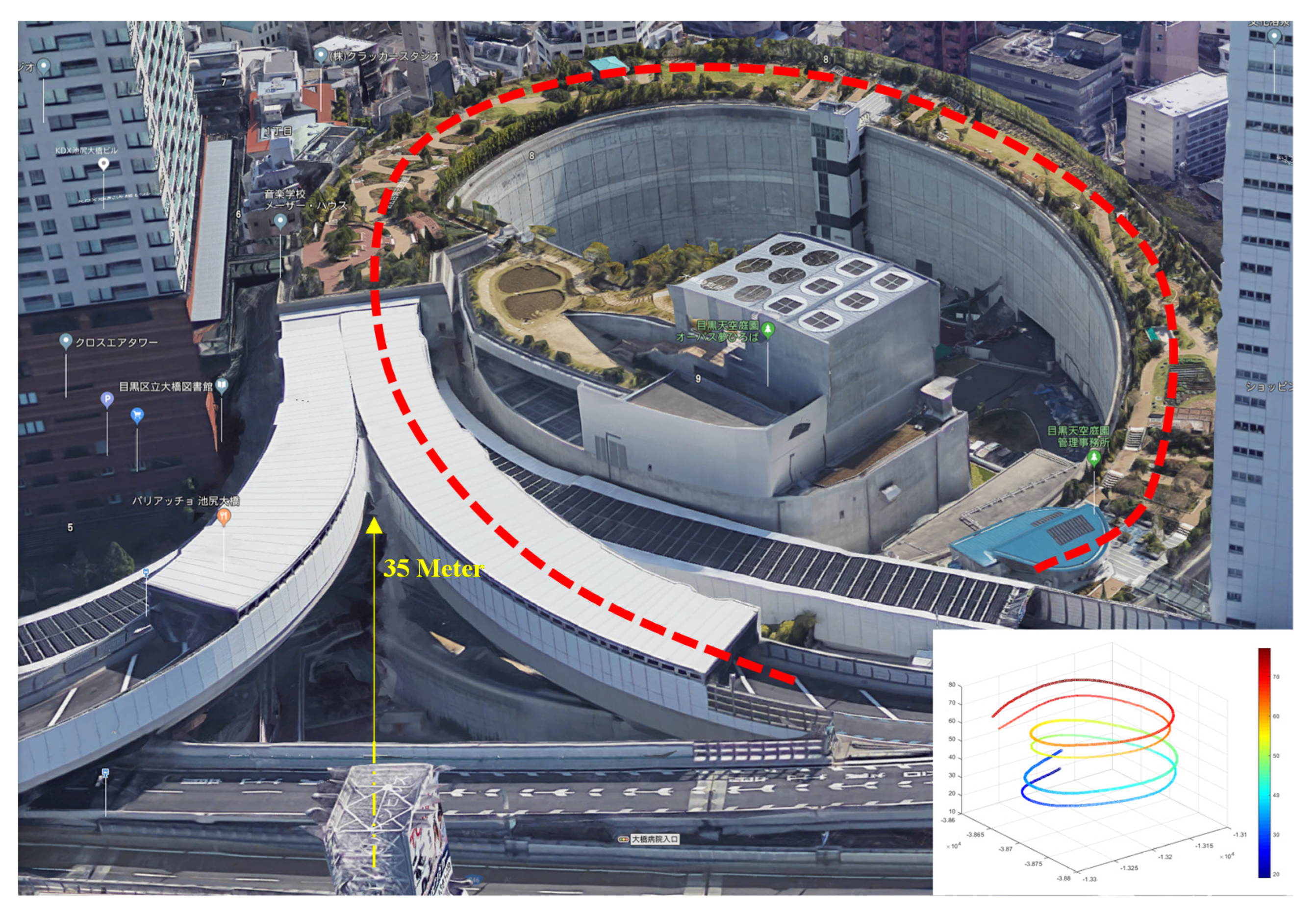
As the main goal of this paper is to emphasize the robustness of the LSM, Ohashi Highway Junction in Tokyo was selected as shown in Figure 9. Ohashi Junction is one of the most complicated traffic nodes in Japan because it contains four stacked loops with a height of 71 m (36 m underground and 35 m of closed sky above ground). Each loop is 400 m lap in an upward/downward driving direction with two lanes of the width of 9.75 m. The maximum slope in the longitudinal direction is 7% whereas it is 10% in the lateral direction. The junction contains two entrances and two exits to drive through each loop in the up/down directions. On 9 October 2021, we drove from Yono Junction towards the Yamate Tunnel which ends with the underground entrance to Ohashi Junction. The upward two loops were then scanned and a U-turn was made shortly after the exit to scan the downward loops and collect the data of the GIR and LIDAR as illustrated in Figure 9.
Before using the LSM, the validation of the accumulation strategy had to be checked with respect to the vehicle trajectory. This was achieved by calculating the difference between the direct post-processed altitudinal vehicle position and the elevation value of the nearest pixel’s error on the map. Figure 10 shows the map-error profile of the trajectory between Yono Junction and the exit of Ohashi Junction. Along this trajectory, the road slope changes considerably at different segments, e.g., two bridges, the Yamate Tunnel and loops between 30 m underground and 35 m above ground. One can observe that the average error is less than 2 cm; this indicates the robustness of the proposed accumulation method as explained in Section 4. However, this reasonable error emerges because of the accuracy of the calibration parameters between the vehicle and LIDAR coordinate systems.
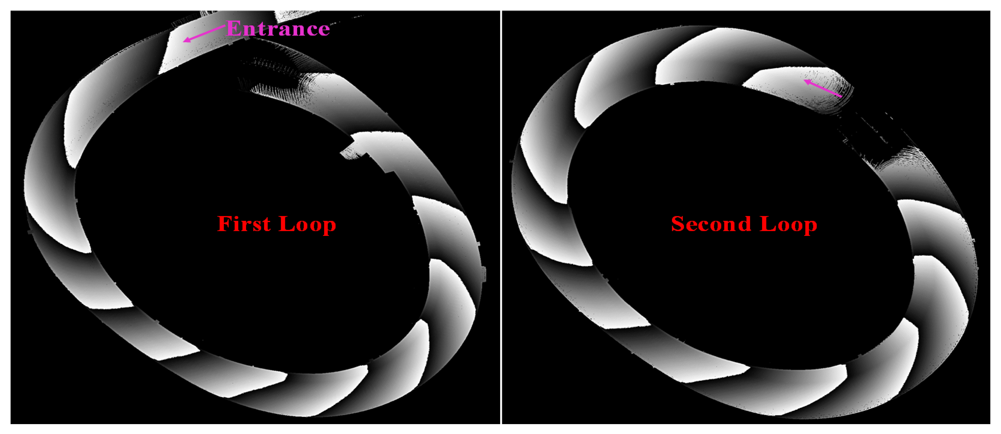
Figure 11 demonstrates the continuous rapid change of the lateral and longitudinal slopes in the first and second upward loops. The images encode the top 200 cm altitude in the road and each bright-dark edge indicates an increment of the height by β. Saving these float changes in a dense pattern is vital to represent the road elevation accurately. Moreover, it is very important to consider the processing time for the map retrieval in such a critical highway junction. These requirements are significantly achieved by the LSM by simply reading BMP images using the IDs (z) to represent the height in the m-order and the pixel values to densely and continuously indicate the cm-order of the road surfaces.
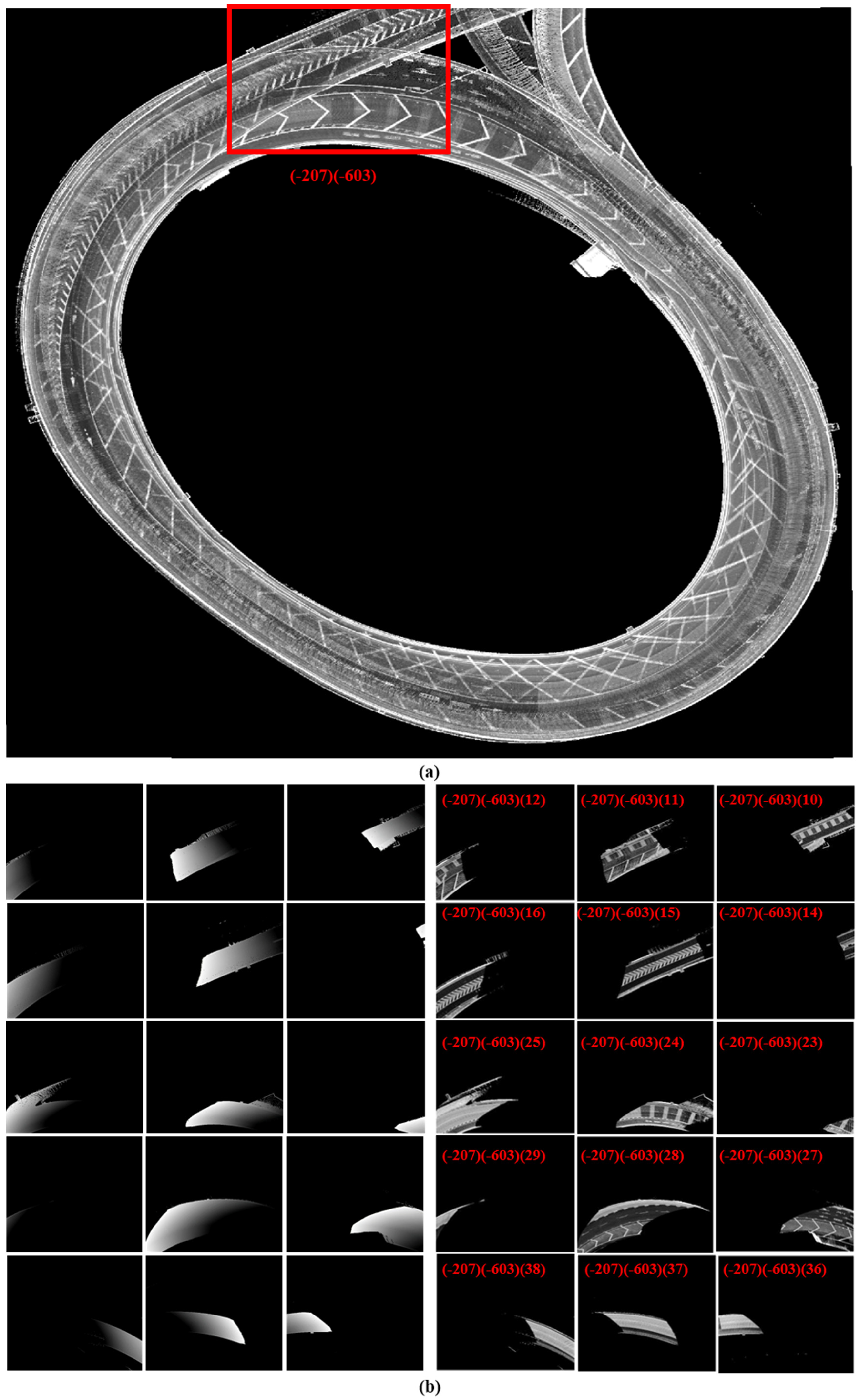
Figure 12a shows a sub-image of a common area of Ohashi Junction that illustrates the accumulation of the four loops with the exit. During autonomous driving, this inaccurate accumulated map image is compared with a LIDAR image of only a unique layer to localize the vehicle in the lateral and longitudinal directions. Therefore, achieving accurate localization is almost impossible and very risky because the map image contains different multiple matching patterns. In contrast, Figure 12b illustrates the efficiency of the LSM to automatically separate and encode the differences in the road texture and structure along the four loops using a set of layered images with the corresponding IDs in the XYZ plane.

6.3. Localization in a Challenging Multilevel Environment Using LSM

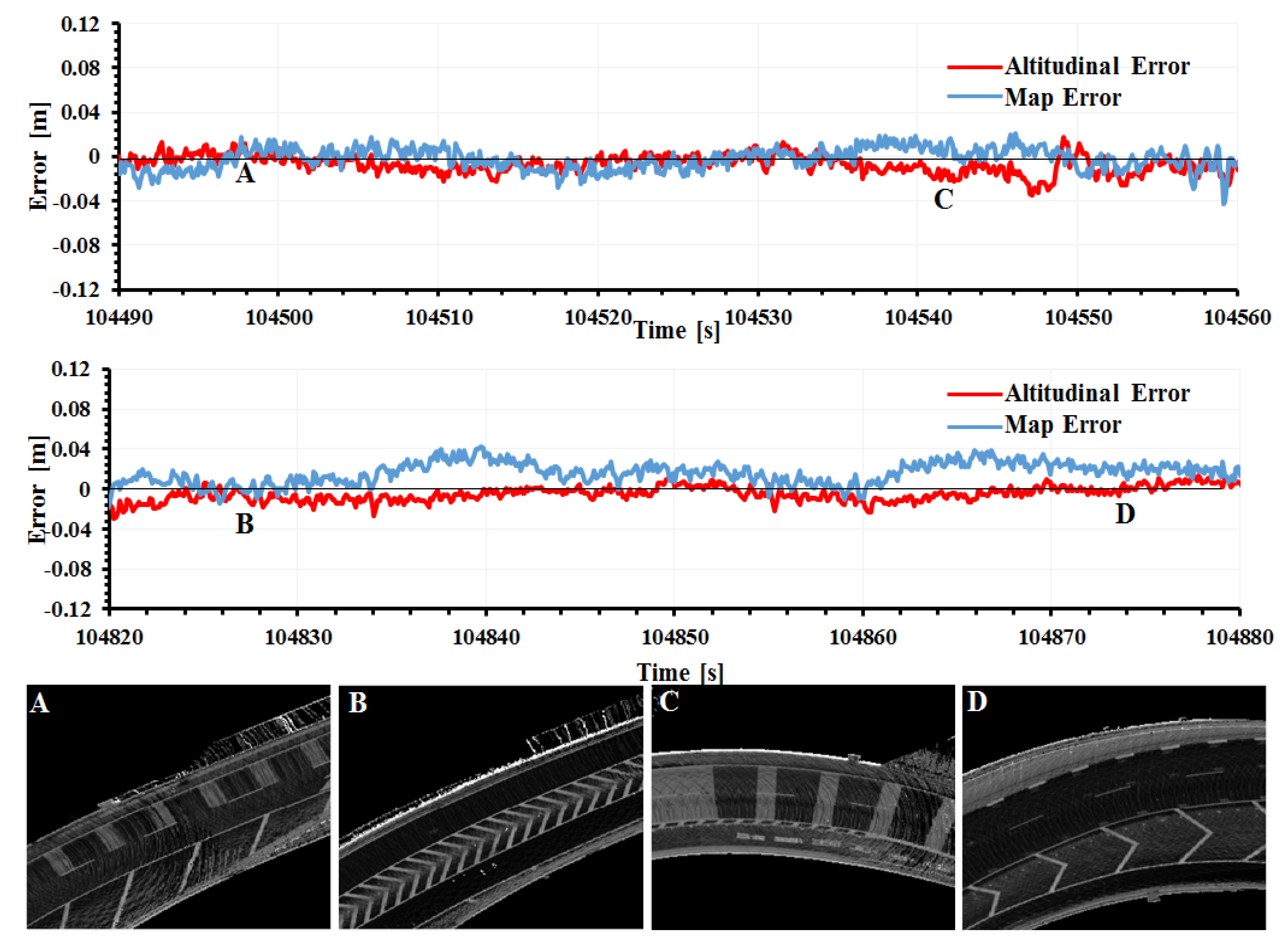
In the proposed LSM-based localization framework, the accuracies in the XY and Z directions influence each other because xy offsets are computed using a map image that is created based on the estimated altitudinal position z. The offset of z is then calculated using the xy estimated position. Figure 13 shows the error profiles of the elevation map and the estimated altitudinal position with respect to the ground truth in the upward and downward two loops, respectively. One can observe the high accuracy of the altitude estimation (around 2 cm). The position error is less than the map error that implies the robustness of the proposed method to relatively compensate the calibration errors between LIDAR and vehicle coordinate systems as well as to recover the slight changes in environments in the Z direction, such as grass on the roadsides. Accordingly, the map images in the four layers are perfectly retrieved and formed during autonomous driving as shown in Figure 13 for the common area in Figure 12b.
Figure 14 demonstrates the localization accuracy in the lateral and longitudinal directions of the estimated positions by DR and the proposed method in the upward and downward loops, respectively. The accuracy of the proposed method is less than 10 cm, whereas 30 m is the average drifting by DR. This indicates the robustness to perfectly retrieve the road surface on each level and compensate the DR errors by a LSM. Accordingly, the scalability and applicability of the LSM and the relevant based localization system have been proved to precisely and safely enable autonomous driving in very critical multilevel environments.
Finally, one can claim that the GIR system may provide low-accuracy measurements in challenging environments because of the obstruction and deflection of the satellite signals, i.e., long tunnels and Ohashi Junction. This significantly influences the map creation and the layer separation. This problem has been robustly solved by proposing a unique Graph-SLAM framework on the node level to generate precise nodes intensity and elevation images (2.5D maps) [26]. Consequently, the proposed LSM strategy in this paper was incorporated into the final stage of the Graph-SLAM framework to generate an accurate LSM.

7. Conclusions

We proposed a robust mapping framework to generate layered sub-image maps in multilevel environments using intensity and elevation LIDAR data. The unique strategy to use the 2D image domain to represent the elevation float values efficiently enabled map retrieval in real time by simply reading images during autonomous driving. This allowed us to encode a dense and continuous representation of the roads’ structures and slopes. Moreover, the identification tactic in the XYZ plane facilitated the update of the map on each layer and add new layers based on the vehicle trajectory. The reliability and efficiency of the proposed framework have been proved by generating the LSM in a very critical multilevel highway junction and accurately localizing the vehicle with average errors of 5 cm and 2 cm in the XY and Z planes, respectively.

Author Contributions

M.A.: Investigation, Methodology, Resources, Software, Validation, Visualization, Writing—original draft, Writing—review and editing and Submission. N.S.: Supervision and Resourcing. R.Y.: Methodology, Investigation, data collection and resources. All authors have read and agreed to the published version of the manuscript.

Funding

This work was partly supported by the Japan Society for the Promotion of Science (KAKENHI Funds: No. 20K19893 and No. 22K17974).

Conflicts of Interest

The authors declare no conflict of interest.

References

  1. Rozenberszki, D.; Majdik, A. LOL: Lidar-only Odometry and Localization in 3D point cloud maps. In Proceedings of the 2020 IEEE International Conference on Robotics and Automation (ICRA), Paris, France, 31 May–31 August 2020; IEEE: Piscataway, NJ, USA; pp. 4379–4385. [Google Scholar]
  2. Murakami, T.; Kitsukawa, Y.; Takeuchi, E.; Ninomiya, Y.; Meguro, Y. Evaluation Technique of 3D Point Clouds for Autonomous Vehicles Using the Convergence of Matching Between the Points. In Proceedings of the 2020 IEEE/SICE International Symposium on System Integration (SII), Honolulu, HI, USA, 12–15 January 2020; pp. 722–725. [Google Scholar] [CrossRef]
  3. Levinson, J.; Thrun, S. Robust Vehicle Localization in Urban Environments Using Probabilistic Maps. In Proceedings of the 2010 IEEE International Conference on Robotics and Automation, Anchorage, AK, USA, 3–5 May 2010; pp. 4372–4378. [Google Scholar]
  4. Wei, L.; Cappelle, C.; Ruichek, Y. Horizontal/vertical LRFs and GIS maps aided vehicle localization in urban environment. In Proceedings of the 16th International IEEE Conference on Intelligent Transportation Systems, The Hague, The Netherlands, 6–9 October 2013; pp. 809–814. [Google Scholar]
  5. Triebel, R.; Pfaff, P.; Burgard, W. Multi-level surface maps for outdoor terrain mapping and loop closing. In Proceedings of the 2006 IEEE/RSJ International Conference on Intelligent Robots and Systems, Beijing, China, 9–15 October 2006; pp. 2276–2282. [Google Scholar]
  6. Lacroix, S.S.; Mallet, A.; Bonnafous, D.; Bauzil, G.; Fleury, S.; Herrb, M.; Chatila, R. Autonomous rover navigation on unknown terrains: Functions and integration. Int. J. Robot. Res. 2002, 21, 917–942. [Google Scholar] [CrossRef]
  7. Nuchter, A.; Lingemann, K.; Hertzberg, J.; Surmann, H. 6D SLAM with approximate data association. In Proceedings of the 12th International Conference on Advanced Robotics, Seattle, WA, USA, 18–20 July 2005; pp. 242–249. [Google Scholar]
  8. Schaefer, A.; Büscher, D.; Vertens, J.; Luft, L.; Burgard, W. Long-Term Urban Vehicle Localization Using Pole Landmarks Extracted from 3 to D Lidar Scans. In Proceedings of the 2019 European Conference on Mobile Robots, Prague, Czech Republic, 4–6 September 2019; pp. 1–7. [Google Scholar]
  9. Lamon, P.; Stachniss, C.; Triebel, R.; Pfaff, P.; Plagemann, C.; Grisetti, G.; Kolski, S.; Burgard, W.; Siegwart, R. Mapping with an Autonomous Car. In Proceedings of the IEEE/RSJ IROS Workshop: Safe Navigation in Open and Dynamic Environments, Beijing, China, 10 October 2006. [Google Scholar]
  10. Kummerle, R.; Hahnel, D.; Dolgov, D.; Thrun, S.; Burgard, W. Autonomous driving in a multi-level parking structure. In Proceedings of the 2009 IEEE International Conference on Robotics and Automation, Kobe, Japan, 12–17 May 2009; pp. 3395–3400. [Google Scholar]
  11. Aldibaja, M.; Suganuma, N.; Yoneda, K. LIDAR-Data accumulation strategy to generate high definition maps for autonomous vehicles. In Proceedings of the IEEE Conference on Multisensor Fusion and Integration for Intelligent Systems, Daegu, Republic of Korea, 16–18 November 2017; pp. 422–428. [Google Scholar]
  12. Aldibaja, M.; Suganuma, N.; Yoneda, K. Robust intensity based localization method for autonomous driving on snow-wet road surface. IEEE Trans. Ind. Informatics. 2017, 13, 2369–2378. [Google Scholar] [CrossRef] [Green Version]
  13. Aldibaja, M.; Suganuma, N.; Yoneda, K.; Yanase, R. Challenging Environments for Precise Mapping Using GNSS/INS-RTK Systems: Reasons and Analysis. Remote Sens. 2022, 14, 4058. [Google Scholar] [CrossRef]
  14. Lee, W.; Cho, H.; Hyeong, S.; Chung, W. Practical Modeling of GNSS for Autonomous Vehicles in Urban Environments. Sensors 2009, 19, 4236. [Google Scholar] [CrossRef] [PubMed] [Green Version]
  15. Nam, T.H.; Shim, J.H.; Cho, Y.I. A 2.5D Map-Based mobile robot localization via cooperation of aerial and ground robots. Sensors 2017, 17, 2730. [Google Scholar] [CrossRef] [PubMed] [Green Version]
  16. Sun, L.; Zhao, J.; He, X.; Ye, C. DLO: Direct LiDAR Odometry for 2.5D Outdoor Environment. In Proceedings of the 2018 IEEE Intelligent Vehicles Symposium (IV), Suzhou, China, 26–30 June 2018; pp. 1–5. [Google Scholar]
  17. Moran, P.; Periera, L.F.; Selvaraju, A.; Prakash, T.; Ermilios, P.; McDonald, J. A 2.5d vehicle odometry estimation for vision applications. In Proceedings of the Irish Machine Vision and Image Processing (IMVIP) Conference, Sligo, Ireland, 31 August–2 September 2020; IEEE: Piscataway, NJ, USA, 2020; pp. 61–68. [Google Scholar] [CrossRef]
  18. Olson, E.; Agarwal, P. Inference on networks of mixtures for robust robot mapping. Int. J. Robot. Res. 2013, 32, 826–840. [Google Scholar] [CrossRef] [Green Version]
  19. Qin, T.; Zheng, Y.; Chen, T.; Chen, Y.; Su, Q. RoadMap: A Light-Weight Semantic Map for Visual Localization towards Autonomous Driving. In Proceedings of the 2021 IEEE International Conference on Robotics and Automation (ICRA), Xi’an, China, 30 May–5 June 2021. [Google Scholar]
  20. Wang, L.; Zhang, Y.; Wang, J. Map-based localization method for autonomous vehicles using 3D-LIDAR. IFAC-Papers OnLine 2017, 50, 276–281. [Google Scholar] [CrossRef]
  21. Wolcott, R.; Eustice, R. Fast lidar localization using multiresolution gaussian mixture maps. In Proceedings of the 2015 IEEE international conference on robotics and automation (ICRA), Seattle, WA, USA, 26–30 May 2015; pp. 2814–2821. [Google Scholar]
  22. Shan, T.; Englot, B.; Meyers, D.; Wang, W.; Ratti, C.; Rus, D. Lio-sam: Tightly-coupled lidar inertial odometry via smoothing and mapping. In Proceedings of the 2020 IEEE/RSJ International Conference on Intelligent Robots and Systems (IROS), Las Vegas, NV, USA, 24 October–24 January 2020; pp. 5135–5142. [Google Scholar] [CrossRef]
  23. Yoon, J.; Kim, B. Vehicle Position Estimation Using Tire Model in Information Science and Applications; Springer: Berlin, Germany, 2015; Volume 339, pp. 761–768. [Google Scholar]
  24. Otsu, N. A Threshold Selection Method from Gray-Level Histograms. IEEE Trans. Syst. Man Cybern. 1979, 9, 62–66. [Google Scholar] [CrossRef] [Green Version]
  25. Nuss, D.; Reuter, S.; Thom, M. A random finite set approach for dynamic occupancy grid maps with real-time application. Int. J. Robot. Res. 2018, 37, 841–866. [Google Scholar] [CrossRef] [Green Version]
  26. Aldibaja, M.; Suganuma, N. Graph SLAM-Based 2.5D LIDAR Mapping Module for Autonomous Vehicles. Remote Sens. 2021, 13, 5066. [Google Scholar] [CrossRef]
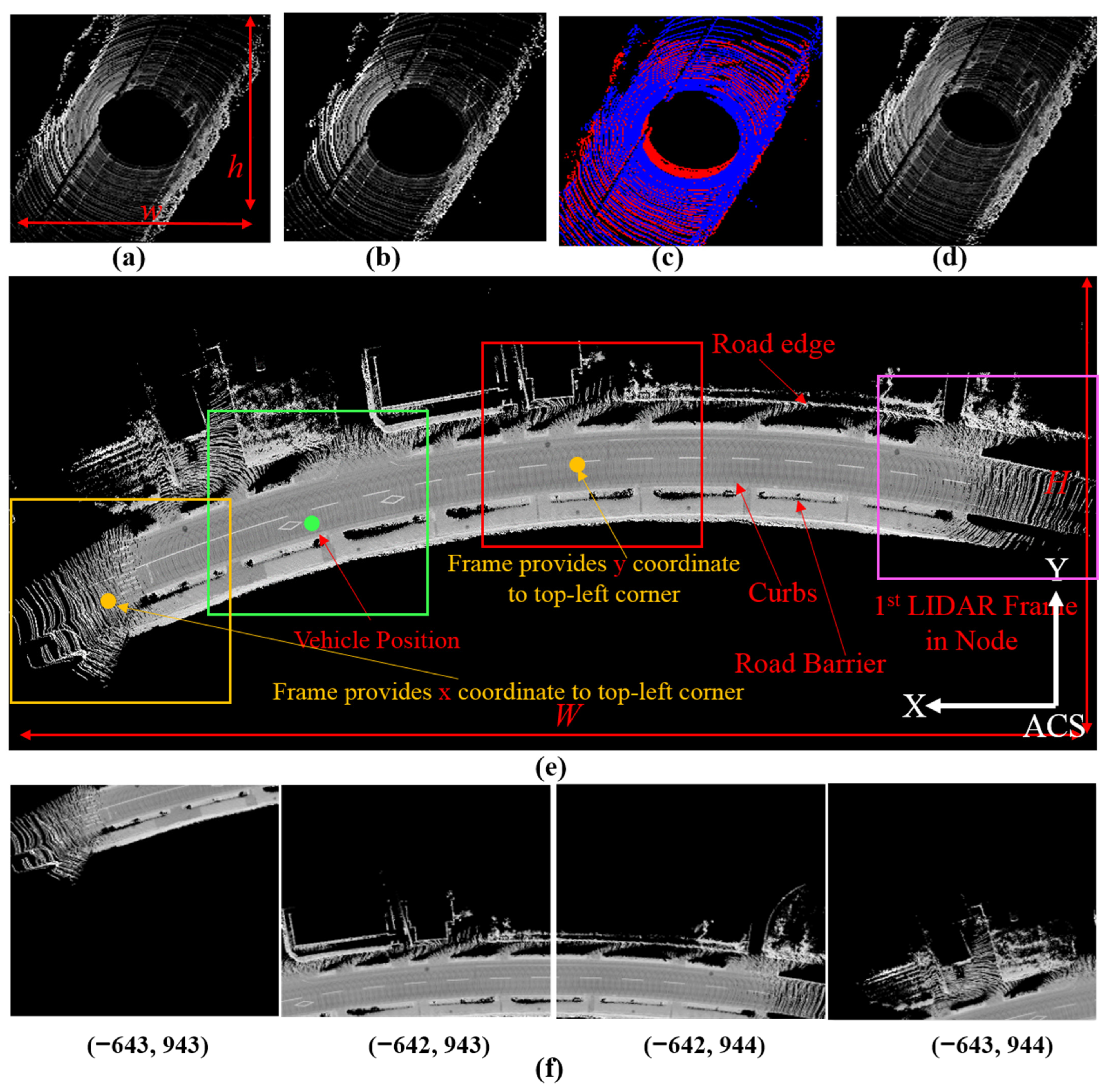
Figure 1. Mapping strategy in node domain. (a) 1st LIDAR frame. (b) 2nd frame. (c) Common pixels. (d) Accumulated image. (e) Node intensity image. (f) Four sub-images in node (e) with global IDs (x, y).
Remotesensing 14 05847 g001
Figure 2. (a) Multilevel environment consisting of three layers: ground-tunnel, bridge-tunnel and mountain surface. (b) The three layers are accumulated in the same map image [8]. (ce) Map image in (b) overlapped by LIDAR image based on the matching score in the three layers, respectively. Red circle and rectangle show the accurate actual location whereas yellow circle indicates the estimated position.
Remotesensing 14 05847 g002
Figure 3. (a) Ground and bridge road structure represented by an elevation map showing the vehicle trajectory. (b) Intensity map consisting of three nodes. (c) Common area between bridge and ground road surfaces. (d) Intensity (top) and elevation (bottom) images of overlapped area.
Remotesensing 14 05847 g003
Figure 4. Ground and bridge road structure shown in Figure 3 are mapped according to LSM. (a) The elevation image of the ground road surface is first encoded and divided into two layers in the pink polygon. The map is then extended in the Z direction based on the Z-IDs to contain the bridge layer images. (b) The corresponding intensity images are created according to the pixel distribution in the layered elevation images in (a).
Remotesensing 14 05847 g004
Figure 5. Map retrieval strategy. (a) Restoring four sub-images of the ground layer in Figure 3 based on the vehicle pose and creating lower and upper virtual planes. (b) Elevation map image created by merging the lower two layered elevation images in Figure 4a. (c) Intensity map image of the ground road surface.
Remotesensing 14 05847 g005
Figure 6. LSM based localization system in XY plane. Lateral and longitudinal offsets are first calculated in XY plane using image matching between intensity map and LIDAR images.
Remotesensing 14 05847 g006
Figure 7. LSM based localization system in the Z plane. Elevation map image is cut off in the same size of LIDAR elevation frame (192 × 192) according to the obtained offsets in XY plane. Histogram between the elevation LIDAR and cut-map images is created and converted into a likelihood vector and then skinned by Sigmoid function to estimate z-offset based on Otsu’s threshold.
Remotesensing 14 05847 g007
Figure 8. Experimental platform with sensor configurations.
Remotesensing 14 05847 g008
Figure 9. Ohashi junction. The 35 m closed sky part aboveground with two driven upward and downward trajectories. The red dotted line demonstrates the vehicle trajectory in the forth loop.
Remotesensing 14 05847 g009
Figure 10. The trajectory between Yono and Ohashi highway junctions with front camera images of ground, bridge, tunnel and entrance of Ohashi.
Remotesensing 14 05847 g010
Figure 11. First and second loops in upward direction representing the top 200 cm of the road height. Bright-dark edges indicate increasing height by 2 m. Road slope is effectively and densely illustrated by grayness changes.
Remotesensing 14 05847 g011
Figure 12. Common area of four loops with the exit segment of Ohashi Junction. (a) Accumulative map image produced by the old mapping system [8]. (b) LSM with corresponding ID: elevation in 200 cm above Z-IDs (left) and intensity (right).
Remotesensing 14 05847 g012
Figure 13. The elevation map error compared to GIR and the altitudinal accuracy in upward and downward trajectories with map images in the common areas (AD) that were retrieved by the proposed localization system based on layered elevation-intensity images. The RMSE errors of the map and altitudinal errors in the upward and downward trajectories are 0.025 m, 0.019 m, 0.029 m and 0.011 m.
Remotesensing 14 05847 g013
Figure 14. Localization in XY plane. (a) Lateral (top) and longitudinal (bottom) errors of the proposed localization system and the DR in the two upward loops compared to GIR ground truth. The RMSE errors of the dead reckoning and proposed localization module in the lateral and longitudinal direction are 0.048 m, 27 m, 0.037 m and 29 m, respectively. (b) Lateral and longitudinal errors in the downward two loops. The corresponding RMSE errors of the dead reckoning and proposed localization module in the lateral and longitudinal direction are 0.087 m, 28.8 m, 0.049 m and 31.2 m, respectively.
Remotesensing 14 05847 g014
Publisher’s Note: MDPI stays neutral with regard to jurisdictional claims in published maps and institutional affiliations.