Abstract
The objective of this study was the estimation of the dynamic evolution of the Planetary Boundary Layer (PBL) height, using advanced remote sensing measurements from Finokalia Station, where the Pre-TECT Campaign took place during 1–26 April 2017. PollyXT Raman Lidar and Halo Wind Doppler Lidar profiles were used to study the daily vertical evolution of the PBL. Wavelet Covariance Transform (WCT) and Threshold Method (TM) were performed on different products acquired from Lidars. According to the analysis, all methods and products are able to provide reasonable boundary-layer height estimates, each of them showing assets and barriers under certain conditions. Two cases are presented in detail, indicating the limited daytime evolution of a coastal area, the decisive role of wind speed-direction in the formation of a shallow or high boundary layer and the differences when using aerosols or turbulence as tracers for the PBL height retrieval. Comparison between the observed PBL and ECMWF model results was made, establishing the importance of actual PBL measurements, in coastal regions with complex topography.
1. Introduction
The Planetary Boundary Layer (PBL) height estimation provides useful information on the available air volume above the Earth’s surface into which emitted air pollutants are diluted and thus is a key parameter in air quality and weather or dispersion forecasting models. Over land surfaces under high-pressure conditions, the boundary layer has a well-defined structure that evolves with the diurnal cycle [1]. The three major components of this structure are the Mixed Layer (ML), the residual layer, and the stable boundary layer. When it comes to coastal regions the daytime evolution can be less pronounced and the formation of an Internal Boundary Layer (IBL) is a common phenomenon. During a sunny day, the sea breeze will blow the stable or neutrally stratified air over the sea towards land. The surface heating effect and dynamic disturbance effect intensify the turbulence in the lowest atmospheric layer to form an unstable layer, which develops into the Thermal Internal Boundary Layer (TIBL) [2]. Also, an IBL can develop when flow over a uniform surface encounters a step-change in surface conditions such as aerodynamic roughness, temperature, or moisture [3]. Moreover, the TIBL characteristics over the coastal land after the onset of the sea breeze are similar to those of the shallow convective boundary layer, commonly observed over plain areas. Therefore, the height of the TIBL can be considered the height of the shallow convective boundary layer [2]. In the case of an offshore wind flow, the internal structure of the IBL can present many similarities with the slowly evolving stable boundary layer overland [4].
Studying PBL in regions with special topography such as steep cliffs, islands, or mountains, highlights the importance of field measurements. In this analysis, the PBL diurnal evolution and characteristics are examined at Finokalia, a coastal region on the northern coast of Crete, Greece, located at the top of a hilly elevation, facing the sea within a sector 270° to 90°. The location of the island, along with the atmospheric circulation patterns [5], form a rich aerosol scene in the area, originating from natural sources (marine aerosols from the Aegean Sea, dust particles from Africa) or anthropogenic activities (pollution from big regional centers such as Istanbul and Heraklion). On a synoptic scale, the Eastern Mediterranean is at the crossroads of air mass outflows from European and Asian pollution sources [6] and receives significant amounts of desert dust from Africa and the Middle East. The region is characterized by considerable variability in cloud systems, ranging from frontal and convective to cyclones [7,8,9]. It is a climate “hot spot”, exhibiting more frequent and more intense weather phenomena associated with severe winds (Etesians), floods, and dust events during the transition seasons [10,11,12,13,14]. Therefore, accurate PBL height is needed to correctly interpret the numerous measurements at the Finokalia site.
The use of Lidar systems for active remote sensing of meteorological parameters and aerosols, is an effective way to detect ML height. Past studies have verified PBL height obtained from Lidar data by using several methods, against PBL height derived from radiosonde data [15,16,17,18,19,20]. Studying ML by means of Lidars, can suffer from many restrictions related to weather conditions, range, and accuracy, but can also provide high temporal and spatial resolution. The retrieval of the PBL top in a region with special topography, can hardly be an automated procedure, because of the variability inserted by aerosols and cloud presence, as well as by strong wind fields. Furthermore, very shallow PBL heights can occur at coastal locations [21]. Baars et al. [15] describe the continuous monitoring of the boundary-layer top with lidars, using several modifications of the Wavelet Covariance Transform, according to the different backscatter conditions in rather clean or very polluted air.
In this study, measurements from collocated PollyXT Raman Lidar and Halo Wind Doppler Lidar, collected during the PreTECT Campaign, were used to investigate the PBL dynamic characteristics. The PreTECT experimental Campaign (described in Section 2) took place in Finokalia, Crete, where remote sensing and in-situ measurements were obtained. Wavelet Covariance Transform (WCT) and Threshold Method (TM), are applied on Lidar products, that work as indicators for the ML. This work contributes to the discussion of PBL evolution and height detection [22,23], comparing methods applied to different metrics for two case studies characterized by different meteorological conditions and through month-long analysis. Comparing field measurements with model results, contributes to the fundamental understanding of the PBL [24,25,26]. In our study, the observed PBL form Lidars is compared with the ERA5 Re-Analysis dataset from European Centre for Medium-Range Weather Forecasts (ECMWF) results.
The manuscript is structured as follows: Section 2 describes the instrumentation, data, and the methodology applied to retrieve the PBL height. Section 3 presents the case studies and the associated meteorological conditions analyzed in detail. The results are discussed along with the statistical analysis performed for PBL height retrievals during the campaign. The main conclusions are summarized in Section 4.
2. Instrumentation, Data, and Methodology
In this study, an ensemble of active remote sensing instrument observations is used in order to derive the PBL height. As mentioned in the introduction, the measurements were collected in the frame of the Pre-TECT Campaign [27] that took place in Finokalia (35.34°N, 25.67°E, 250 m a.s.l.) (Figure 1), Crete, during the period 1–26 April 2017, organized by the National Observatory of Athens (NOA). Observations from PollyXT Raman Lidar [28] and a Halo scanning Wind Doppler Lidar [29], are also processed. Wavelet Covariance Transform and Threshold Method are applied with several modifications to the products of the campaign dataset.
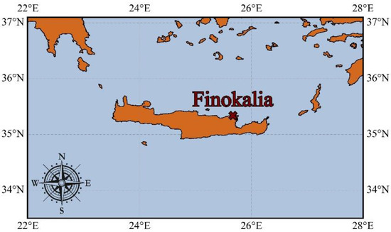
Figure 1.
Finokalia station (35.34°N, 25.67°E, 250 m a.s.l.) on the north coast of Crete.
2.1. Instrumentation
This section gives an overview of the two active remote sensing instruments operating during the PreTECT campaign.
The multi-wavelength depolarization, Raman PollyXT Lidar of the National Observatory of Athens (NOA), was built in 2014 and operated in Athens (2015–2016), Nicosia (for 2 campaigns in March 2015 and April 2016), Finokalia (2017–2018) and Antikythera (2018–today). The system components are briefly depicted in Table 1, but a more detailed description can be found in [28]. PollyXT Lidar consists of a compact, pulsed Nd:YAG laser, emitting at 355, 532, and 1064 nm at a 20 Hz repetition rate, with the laser beam pointed into the atmosphere at an off-zenith angle of 5°. The backscattered signal is collected by a Newtonian telescope with a 0.9 m focal length, acquiring profiles with a vertical resolution of 7.5 m, and a temporal resolution of 30 s. The system includes five elastic channels for far and near range detection at 355, 532, and 1064 nm; four Raman channels for far and near range detection at 387 and 607 nm; two depolarization channels at 355 nm and 532 nm; and a water vapor channel at 407 nm. The overlap-affected height range of the overall system is 120 m above the lidar for the Near Field channels and between 700 and 800 m height for the Far Field channels. All measurements within the period 2014–2022 are available online at http://polly.tropos.de (accessed on 15 August 2022).

Table 1.
Specifications of PollyXT Raman Lidar, more information at [28].
The Halo Photonics Stream Line Scanning Doppler lidar, is a 1.5 µm pulsed Doppler lidar with a heterodyne detector that can switch between co- and cross-polar channels [25]. The Doppler lidar has a range resolution of 30 m and measures the attenuated aerosol backscatter and Doppler velocity along the beam direction. Two conical scans at 15° and 75° elevation angle and a 3° elevation angle sector scan were scheduled every 15 min. This schedule leaves approx. 9 min out of every 15 min for vertically-pointing measurement. For the vertically-pointing measurements integration time was set to 3.7 s. For the 15° conical scan integration time was 4.5 s and for the 75° conical scan integration time was 6.5 s. More details about Halo Doppler Lidar characteristics and specifications can be found at [29,30]. The technical specifications of the instrument as configured for standard operation during the campaign are summarized in Table 2.
Table 2.
Specifications of Halo Wind Lidar, more information at [29].
2.2. Data
For the case studies analyzed herein, several products are retrieved from each instrument. Range Corrected Signal (RCS), attenuated BackSCatter coefficient (BSC) and Water Vapor Mixing Ratio (WVMR) are calculated from the PollyXT Lidar, using the signal from 532 nm Near Field (NF) and 1064 nm Far Field (FF) channel for the BSC product and the ratio of 387 nm and 407 nm signals for the WVMR product [31]. WVMR profiles from PollyXT lidar are calibrated by the collocated Microwave Radiometer (MWR) [32,33]. The WVMR retrievals are only available during nighttime hours, 00:00–04:00 and 18:00–24:00 UTC.
The Halo Doppler Lidar measurements were post-processed according to [30,34,35] and an SNR-threshold of 0.0075 was applied to the data. Horizontal wind speed and direction were retrieved from the conical scans [36] and turbulent kinetic energy dissipation rate (TKEdr) was estimated following [37]. Both Lidars are placed at 252 m above sea level.
For the meteorological analysis of the case studies, the ERA5 Re-Analysis dataset from European Centre for Medium-Range Weather Forecasts (ECMWF) is used [38], at 0.25° × 0.25° resolution with 137 levels [39]. The ERA5 reanalysis model defines the PBL height as the minimum height for the bulk Richardson number reaching the critical value of 0.25, according to the algorithm that was proposed by Vogelezang and Holtslag [40] and is publicly available through the Copernicus Climate Data Store (CDS) [41]. For the vertical meteorological parameters needed for the retrieval of WVMR from PollyXT Lidar, we utilize the Advanced Research Weather Research and Forecasting model version 4.2.1 (WRF-ARW) [42]. The WRF-ARW spatial set up was at 9 × 9 km resolution domain with 600 × 370 grid points and 33 vertical levels. Simulations were initiated at 00:00 UTC on 1 April 2017 and were completed at 18:00 UTC on 30 April 2017. Finally, the atmospheric transport modeling used in this study, is based on the FLEXPART v10.4 (FLEXible PARTicle) Lagrangian dispersion model [43,44]. The following are reproduced:
- (a)
- 8-day air masses back-trajectories prior to their arrival at 2 altitudes (0.5 and 5 km) above Finokalia ground station on 10 April 2017 at 10:00 UTC and
- (b)
- 5-day air masses back-trajectories at 500 m above Finokalia ground station on 14 April 2017 at 10:00 UTC.
The footprint output from FLEXPART, is calculated in unit second (s) according to [44,45]. These specific periods, were chosen to describe the aerosol scene of the cases examined in detail (described in Section 3). The altitudes (500 m, 5 km), correspond to the observed aerosol layers, in order to provide information about their origin and trajectory.
A total of 50,000 particles are released over the Finokalia station in both simulations described above. FLEXPART was driven with 3-hourly meteorological data from the National Centers for Environmental Prediction (NCEP) Global Forecast System (GFS) analyses provided at 0.5° × 0.5° resolution and for 41 model pressure levels.
2.3. Methodology
Wavelet Covariance Transform (WCT) is applied on 532 nm NF RCS and WVMR profiles acquired from PollyXT Lidar and on BSC profiles from Halo Lidar. RCS and BSC are proportional to the air concentration (molecules and aerosols). Threshold method (TM) is applied on TKEdr profiles from Halo Lidar. All the product profiles used in this study, are time-averaged with a 15-min mean, with the exception of TKEdr profiles where a 1-h median is calculated.
2.3.1. Wavelet Covariance Transform (WCT)
The WCT method applied to the above-mentioned products, assumes that the majority of aerosol particles are contained in the PBL, rather than in the free troposphere. Hence, a strong decrease of the signal is observable at ML top. The wavelet covariance function is calculated for every single averaged profile according to the following formula [46]:
f(z) is the signal to perform WCT (in this case it is RCS, BSC, or calibrated WVMR), z is the measurement height, zb and zt are the lower and upper limits of the signal profile, respectively. The dilation a is the extent of the step function (window) and the translation b determines the location of the step.
A critical detail for the accurate WCT application, is the selection of an appropriate value of the dilation so as to distinguish PBL, cloud layers, and aerosol layers [15]. For the examined cases, sensitivity studies were performed, resulting in different dilations, and an algorithm was developed to detect the maxima of the time-averaged vertical profiles for each product. In Figure 2, an example of wavelet signal profiles of 14 April 2017 02:00 UTC is presented (blue color), along with the corresponding product from PollyXT and Halo Lidar, showing the detection of the peak around 400 m. The selection of a fixed dilation of 20·Δz = 150 m, where Δz corresponds to the lidar vertical resolution 7.5 m, works well for the cases of this study.
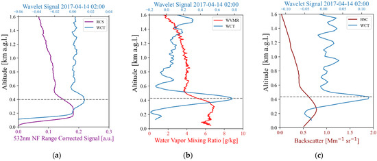
Figure 2.
Wavelet Signal (Blue lines) from 14 April 2017 02:00 UTC, for (a) 532 nm Near Field channel Range Corrected Signal (purple line) from PollyXT Lidar, (b) Water Vapor Mixing Ratio (red line) from PollyXT Lidar and (c) Attenuated Backscatter Coefficient (brown line) from Halo Lidar.
2.3.2. Threshold Method
The Threshold Method (TM) is based on a set of a condition that includes a constant threshold value. More specifically, the TM is applied on the 1-h median TKEdr (ε) profiles as follows: starting from the lowest usable range gate, as high up as TKEdr is larger than the threshold value, the range is considered to lie within the mixing layer. Therefore, the altitude corresponding to this threshold value is interpreted as the turbulent Mixing Layer Height (MLH). For our cases, MLH is determined using the threshold of 10−4 m2·s−3, as suggested in previous studies [21].
The products from each instrument and the method that is applied in each case, are presented in Table 3.
Table 3.
Instruments-Products-Methods, abbreviations are presented at the end of the manuscript.
2.3.3. Comparison between WCT and TM Applied Methods
The methods used in this study in order to retrieve PBL height, present similarities, and differences. WCT detects a strong decrease of the signal of a parameter, while TM detects the first value that overpasses the threshold set by the user. The systematic differences that may arise during inter-comparison of the methods in this study, are attributed to the different parameters on which each method is applied. WCT is used for the detection of PBL height, using aerosols (RCS, BSC, WVMR) as tracers, while TM is used for the detection of PBLH, using a thermodynamic parameter (TKEdr) as tracer. In Figure 3, profiles of products are presented, along with the method used, for 10 April 2017, 01:30 UTC. As observed, WCT captures a layer around 950 m, but TM detects the first point that is lower than the threshold at 790 m approximately. This difference is attributed to the scientific parameter that is used as an indicator for the PBL or MLH height.
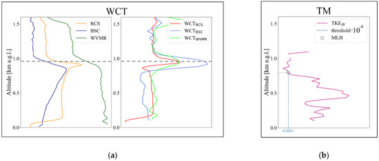
Figure 3.
10 April 2017 01:30 UTC (a) WCT Method: Range Corrected Signal (orange line), attenuated Backscatter Coefficient (blue line) and Water Vapor Mixing Ratio (green line) on the left, Wavelet Signal Profiles (red, light blue, light green line for each parameter, respectively) on the right. (b) Threshold Method (TM): Turbulent Kinetic Energy dissipation profile (purple line) and vertical line (blue dashed) at the set threshold 10−4.
3. Results
Before analyzing statistics of PBL height at Finokalia during the PreTECT Campaign, two days are presented with different meteorological conditions and aerosol mixtures. Firstly, 10 April 2017 is described by the presence of clouds and aerosols and secondly, 14 April 2017, is a day without clouds and significant aerosol load. In Figure 4, wind conditions are illustrated. For the first case, mostly N/NW moderate winds are dominant (Figure 4a) in addition to the second case, where W winds are present up to 600 m, turning to NW above (Figure 4b). The main wind flow in Finokalia is from the North, considering that it is an island in the south Aegean Sea, affected by the Etesians. The presence of Crete Island functions as an obstacle and shifts the wind to NW and W near the surface.
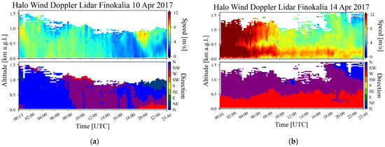
Figure 4.
Time-Height Cross Section of top: Wind Speed and bottom: Wind Direction from Halo Wind Doppler Lidar for (a) 10 April 2017, (b) 14 April 2017. Wind directions depicted in the color bar are classified in degrees as follows: [North: 0°, NW: 45°, W: 90°, SW: 135°, S: 180°, SE: 225°, E: 270°, NE: 315°, N: 360°].
3.1. Case 10 April 2017
3.1.1. Meteorological Analysis
The existence of Azores high over the north Atlantic Ocean and a deep trough over the Black Sea forces the atmospheric mesoscale circulation in Eastern Balkans and therefore, the weather conditions in Greece on this day. The movement of the polar jet stream southwards in Europe, which started in 7 April 2017, permitted colder air masses to enter Eastern Europe and spin with the support of the associated trough system. As shown in Figure 4a, the low-pressure system is located over the Black sea at 500 hPa, accompanied by the colder air mass, presented at 850 hPa with a temperature of 0 °C (Figure 5b).
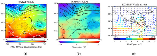
Figure 5.
ECMWF Reanalysis Data for 10 April 2017, 06:00 UTC (a) 500 hPa Geopotential Height (black lines), MSLP (white lines), 1000–500 hPa Thickness, (b) 850 hPa Geopotential Height (black lines), 850 hPa Temperature, (c) 10 m Wind Speed and Direction.
As a result, the weather in Crete, Greece is characterized by low temperatures, favoring cloud formation. The wind field in the Aegean Sea is mostly N/NE, stronger in the central and southern parts reaching up to 12 m/s (6 Beaufort-fresh to a strong breeze, Figure 5c).
On 10 April 2017, sparse high-level (8–10 km) and mid-level (5–8 km) clouds are observed above Finokalia Station, as shown in Figure 5a, depicting the attenuated BSC coefficient at 1064 nm (upper panel) and the volume depolarization ratio (bottom panel) from PollyXT Lidar. Low level (0–2 km) clouds also form inside and above the PBL. The thin aerosol layer observed at 5–6 km presents a depolarization ratio of 15–30% (Figure 6b) and according to the FLEXPART model, originates from NW Africa (green line Figure 6c,d) which suggests a mixture of dust and pollution aerosols. Moreover, marine and pollution aerosols with a volume depolarization ratio of 5–10% exist up to 700 m, coming from the Balkans and the Aegean Sea (blue line Figure 6c,d).
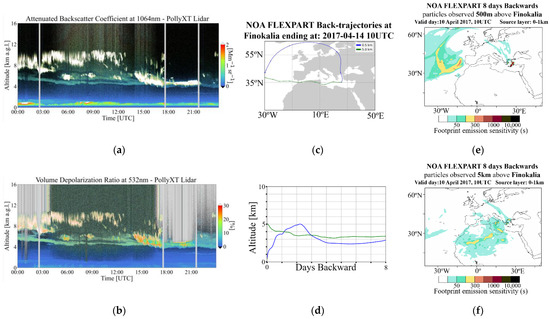
Figure 6.
(a,b) PollyXT Lidar parameters for 10 April 2017 00:00–24:00 UTC: Attenuated Backscatter Coefficient at 1064 nm channel in arbitrary units (a.u.); Volume Depolarization Ratio in percentage units, (c) Air mass backward trajectories, based on FLEXPART simulations, ending at 0.5 (blue) and 5 (green) km above the Finokalia station on 10 April 2017 at 10:00 UTC (d) Altitudes, above ground level, of the air masses on their route prior their arrival over the ground station (e,f) FLEXPART Source–Receptor Relationships (s) for air masses originating from 0–1 km a.s.l. arriving above Finokalia at: 0.5 and 5 km accordingly on 10 April 2017, 10:00 UTC.
3.1.2. PBL Diurnal Evolution on 10 April 2017
Winds from the northern sector (NNW and NNE) are dominant during the entire day, as shown in Figure 4, stronger from 00:00 to 14:00 UTC (up to 8 m/s), compared to the afternoon. A shift in wind direction is observed after 18:00 UTC: west-northwesterly (W/NW) winds reach up to 300 m, switch to north-northeasterly (N/NE) above 700 m, similar to a land breeze.
PBL height is retrieved by applying WCT on the RCS from the 532 nm Near Field channel (Figure 7a—brown circles) and the WVMR (Figure 7c—green triangles) from PollyXT Lidar, as well as on the attenuated BSC from Halo Wind Lidar (Figure 7b—blue circles), resulting to PBLRCS, PBLWVMR, PBLBSC, respectively. The TM is applied on the TKEdr, provided by Halo (Figure 7d—red stars), resulting in MLHTKE retrievals. At the beginning of the day (00:00–04:00 UTC), PBLBSC, PBLWVMR, and PBLBSC, reach up to 1km and then drop gradually to 400 m until 03:00 UTC, whereas MLHTKE, reaches 800 m and then drops to 300 m. During 03:00–11:00 UTC, PBL (where available) presents a rising tendency, from 400 m to 1 km, corresponding to the daytime evolution. After 11:00 UTC, the PBLRCS and PBLBSC is descending from 1 km to 600 m until 18:00 UTC, presenting some local peaks in the meantime. MLHTKE follows that descending from 1 km to 500 m between 10:00–17:00 UTC. After 18:00 UTC, an aerosol layer with top ranging from 500 to 800 m is observed from WCT on RCS, WVMR, and BSC products.
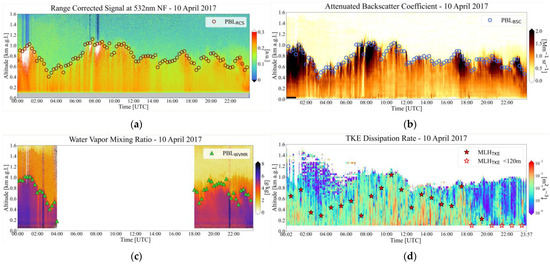
Figure 7.
PollyXT Lidar (a,c) and Halo Wind Doppler Lidar (b,d) products for 10 April 2017: (a) Range Corrected Signal (RCS) at 532 nm NF channel (Grey color at the bottom of the Figure, identifies the incomplete overlap of PollyXT Lidar)—Brown circles: PBL height from Wavelet Covariance Transform (WCT) on RCS (PBLRCS); (b) Attenuated Backscatter Coefficient (BSC)—Blue circles: PBL height from WCT on BSC (PBLBSC); (c) Water Vapor Mixing Ratio (WVMR)—Green Triangles: PBL height from WCT on WVMR (PBLWVMR); (d) Turbulent Kinetic Energy dissipation rate (TKEdr)—Red stars: Mixing Layer Height (MLH) from Threshold Method (TM) on TKEdr (MLHTKE).
In Figure 8, the PBL height and MLH retrievals for 10 April 2017 are compared. At the beginning (00:00–02:00 UTC), all approaches capture a high nocturnal mixing layer. This is probably the result of mechanical turbulence induced by the northerly winds, meeting the coastline. Aerosols and water vapor are transported above the site (as explained in Section 3.1.1), by the same flow and track the mixing layer indicated by TKEdr. After 02:00 UTC, the descending tendency of PBL is captured from all products, as well as the daytime evolution that takes place after 04:00 UTC, when the sun rises and thermal turbulence starts to form. During daytime (05:00–16:00 UTC), PBLRCS and PBLBSC, present accordance in capturing a well-mixed layer reaching 1000 m, which is probably a result of both mechanical and thermal turbulence. However, comparing PBLRCS, PBLBSC, and PBLWVMR with MLHTKE result in some significant differences. PBL from all products, track a higher layer during the entire day, in addition to MLHTKE which tracks the dynamically or thermally turbulent layer, which is significantly dropping after 18:00 UTC. According to [3], the region of significant turbulence is associated with a mesoscale circulation superimposed on the mean offshore flow, and probably relates to a sea-breeze-type circulation. In this case, MLHTKE captures a TIBL that is developed from 02:00 to 17:00 UTC and presents many similarities to a convective boundary layer. Hence the local peak observed at 10:30 UTC is common for both PBL and MLH retrievals. The remarkable difference that is observed after 18:00 UTC, is attributed to the wind direction change, from west (W) winds at the lower layer (at 100 m a.g.l. approximately, Figure 4a) to the north (N) winds at the upper layer, indicating highly stable conditions. The layer near the surface from 18:00 UTC onwards, is directly affected by the land and becomes cooler during the night, while above 300 m the wind flow is from the sea (warmer) and contributes to the continuous transfer of aerosol load and water vapor above Finokalia, used as tracers from the WCT method. This is probably related to land-breeze-type flow, favoring the development of a stable IBL, represented by MLHTKE. Also, WCT on aerosol tracers detects a layer that is rich in aerosols and probably coincides with the residual layer, without following the above-mentioned MLHTKE drop (similar to e.g., [47]) that conceives a stable IBL. PBL from the other products reflects a layer, that is not affected by turbulent transport of surface-related properties and hence does not fall within the nocturnal boundary layer.
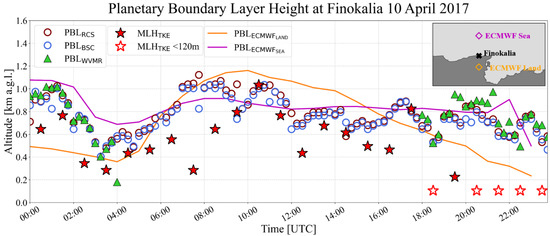
Figure 8.
10 April 2017 PBL height diurnal evolution from WCT applied on 532 nm NF RCS (brown circles—PBLRCS), WVMR from PollyXT Lidar (green triangles—PBLWVMR), BSC from Halo Lidar (blue circles—PBLBSC) and TM applied on TKEdr from Halo Lidar (red stars—MLHTKE). Top right: map with Finokalia’s location between ECMWF Land bin (orange diamond) and ECMWF Sea bin (purple diamond).
The PBL height estimated by the ECMWF model, is presented in Figure 8 for two points that belong in different grids: the purple diamond (PBLECMWFSEA) belongs to a grid simulated over the sea and the orange diamond (PBLECMWFLAND) belongs to a grid simulated over land. Finokalia Station, is located between the two model bins. It is noted that the PBL height derived from ERA5 ECMWF (see Section 2.2), is referred to as ground level, similarly to the PBL height derived from Lidars. During all day, there is good agreement between PBLECMWFSEA and PBL height measured by the instruments. PBLECMWFSEA does not present a sharp daytime evolution, in addition to PBLECMWFLAND which ascents between 04:00–10:00 UTC and descents after 14:00 UTC. Nighttime (00:00–04:00 UTC, 18:00–24:00 UTC) measurements of PBL height are in sufficient agreement with the PBLECMWFSEA. On the other hand, daytime measurements are found to agree mostly with the rising tendency that PBLECMWFLAND presents (04:00–08:00 UTC), but there is a discordance after 16:00 UTC, where PBLECMWFLAND drops very smoothly. MLHTKE, also captures this drop, since the stable IBL is formed in common behavior as a stable nocturnal layer.
3.2. Case 14 April 2017
3.2.1. Meteorological Analysis
On 14 April 2017, zonal flow is restored above Europe, with the polar jet stream limited in the northern paths (500 hPa Figure 9a). Warmer air masses are approaching the Mediterranean Sea with temperatures ranging from 10–15 °C at the 850 hPa level (Figure 9b). Under these atmospheric conditions, the weather in Crete is sunny and warmer. The W/NW wind field that dominates the southern parts of the Aegean (Figure 9c), does not exceed 12 m/s all day.
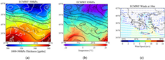
Figure 9.
ECMWF Reanalysis Data for 14 April 2017, (a) 18:00 UTC 500 hPa Geopotential Height (black lines), MSLP (white lines), 1000–500 hPa Thickness, (b) 18:00 UTC 850 hPa Geopotential Height (black lines), 850 hPa Temperature, (c) 06:00 UTC 10 m Wind Speed and Direction.
Regarding the cloud and aerosol conditions on 14 April 2017, skies are cloudless all day above Finokalia station, according to the attenuated BSC coefficient derived from PollyXT Lidar (Figure 10a). The aerosol concentration is very low; probably a mixture of marine and pollution particles with a depolarization ratio of less than 10% (Figure 10b), originating from NW (Figure 10c–e), are present in the lower levels.
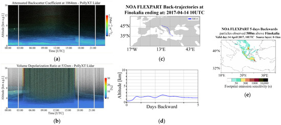
Figure 10.
(a,b) PollyXT Lidar parameters for 14 April 2017 00:00–24:00 UTC: Attenuated Backscatter Coefficient at 1064 nm channel in arbitrary units (a.u.); Volume Depolarization Ratio in percentage units, (c,d) Air mass backward trajectories, based on FLEXPART simulations, ending at 500 m above the Finokalia station on 14 April 2017 at 10:00 UTC; Altitudes, above ground level, of the air masses on their route prior their arrival over the ground station, (e) FLEXPART Source Receptor Relationships (s) for air masses originating from 0–1 km a.s.l. arriving above Finokalia at 500 m on 14 April 2017, 10:00 UTC.
3.2.2. PBL Diurnal Evolution on 14 April 2017
The second case examined, 14 April 2017, is a day with much stronger winds, especially at the beginning of the day, in comparison with 10 April 2017. At the lower levels (below 500 m), the W wind field prevails, with a speed exceeding 15 m/s, in addition to the higher levels (above 500 m), affected by N/NW winds (Figure 4b). After 08:00 UTC, winds above 500 m decrease significantly, but the vertical difference in wind direction is maintained throughout the day. A low-level jet is present throughout the day with peak height at approx. 200 m a.g.l. Overall, the vertical profile of horizontal wind indicates persistent layering, which suggests different characteristics of the air masses at the surface and above 500 m a. g.l.
Before sunrise (00:00–04:00 UTC), WCT on RCS, BSC, and WVMR products, locate a layer around 400 m (Figure 11a–c), while MLHTKE is captured between 200 and 350 m (Figure 11d). After 04:00 UTC, daytime evolution takes place and the PBL starts rising as captured by RCS and BSC products and then drops again after 06:00 UTC to 200 m with small fluctuations. TKEdr from Halo, records a very turbulent layer below 400 m during all day, likely caused by mechanical turbulence generated by the W winds (Figure 4b). During the daytime (05:00 to 14:00 UTC), there is also another turbulent layer present, reaching from 400 m to up to 800 m a.g.l., but this layer seems to be unconnected to the surface, because of the decrease of turbulence at 400 m. Moreover, the lower detected layer is rich in water vapor, reaching around 400 m before sunrise and 200 m after sunset (Figure 11c). As described in Section 2.2, only nighttime measurements of water vapor are available.
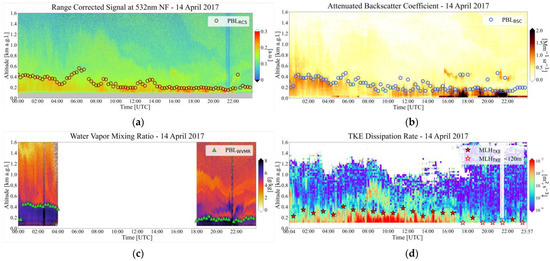
Figure 11.
PollyXT Lidar (a,c) and Halo Wind Doppler Lidar (b,d) products for 14 April 2017: (a) Range Corrected Signal (RCS) at 532 nm NF channel (Grey color at the bottom of the Figure, identifies the incomplete overlap of PollyXT Lidar)—Brown circles: PBL height from Wavelet Covariance Transform (WCT) on RCS (PBLRCS); (b) Attenuated Backscatter Coefficient (BSC)—Blue circles: PBL height from WCT on BSC (PBLBSC); (c) Water Vapor Mixing Ratio (WVMR)—Green Triangles: PBL height from WCT on WVMR (PBLWVMR); (d) Turbulent Kinetic Energy dissipation rate (TKEdr)—Red stars: Mixing Layer (MLH) Height from Threshold Method (TM) on TKEdr (MLHTKE).
Examining all the results together (Figure 12), indicates a significant accordance between all methods and retrievals with a slightly lower MLHTKE. The vertical profile of each product presents a strong decrease, detected by WCT and TM, resulting in strong agreement between the different products. When the sun rises (after 04:00 UTC), weak daytime evolution takes place, with the PBL height and MLHTKE captured by the two Lidars, being in sufficient agreement. Some profiles of Halo BSC and PollyXT RCS, capture a layer around 400 m after 16:00 UTC. This could happen because the northern winds that are imposed from the synoptic system, are modified by the surface due to the presence (obstacle) of Crete and slightly switch to western direction (Figure 4b). As a result, lifting marine and pollution aerosols on the site, are detected by WCT method and causing the outliers of PBLRCS, PBLBSC. Also the PBLRCS and PBLBSC anomalies after 06:00 UTC are very likely to be connected with the wind speed local minimum at 400 m, shown in Figure 3b. After 18:00 UTC, the MLHTKE is mainly detected below 120 m, but PBL from all products is located around 200 m. This indicates the possibility of a stable TIBL formed when there is a slight weakening of wind speed below 200 m (Figure 4b).
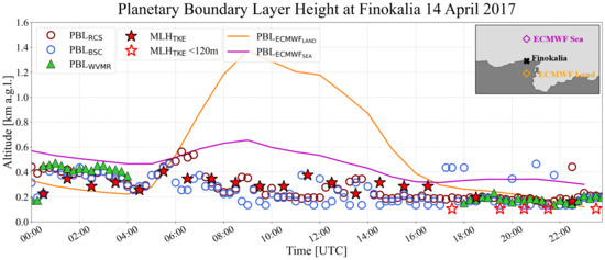
Figure 12.
14 April 2017 PBL height diurnal evolution from WCT applied on 532nm NF RCS (brown circles—PBLRCS), WVMR from PollyXT Lidar (green triangles—PBLWVMR), BSC from Halo Lidar (blue circles—PBLBSC) and TM applied on TKEdr from Halo Lidar (red stars—MLHTKE). Top right: map with Finokalia’s location between ECMWF Land bin (orange diamond) and ECMWF Sea bin (purple diamond).
Furthermore, comparing our results with the ECMWF retrievals, there is a slight underestimation of PBLECMWFLAND at the beginning of the day (00:00–04:00 UTC) and good agreement at the end (18:00 UTC onwards). The underestimation occurs because lidars detect aerosols trapped in the boundary layer, whereas the model predicts a lower nocturnal layer above land. On the other hand, MLHTKE is closer to the PBLECMWFLAND at the beginning of the day, as it represents a lower turbulent layer. PBLECMWFSEA presents the same tendency as PBLWVMR, PBLRCS and PBLBSC during 00:00–04:00 UTC, but deviates after 16:00 UTC, maintaining the values of the nocturnal layer (around 400 m). This overestimation of PBLECMWFSEA is closer to the outliers of PBLBSC and PBLRCS. Nevertheless, a substantial difference arises from 06:00 to 16:00 UTC, with the model’s overestimated PBLECMWFLAND related to lidar retrievals during the convective daytime period. As expected, PBLECMWFSEA is not developing as quickly and is in better accordance with the measurements, still overestimating the measured PBL during 07:00–16:00 UTC. This divergence between PBLECMWFSEA, PBLECMWFLAND and the measurements, especially during daytime, is attributed at the complexes induced by Finokalia’s location. The station is at the edge of a steep cliff between the land and sea, but the model conceives a land surface with high convective activity in case of PBLECMWFLAND and a maritime area in which the marine atmospheric boundary layer forms in case of PBLECMWFSEA. The influence of changes in surface roughness at Finokalia station, occurs at a scale that is too fine for the model, hence the above-mentioned differences arise. It is likely that the continuous on-shore flow yields a vertical profile over the coast on land that closely resembles the maritime near-shore environment, whereas the model’s surface fluxes are likely insensitive to this advection as the surface fluxes are typically one-dimensional based on surface properties.
3.3. Statistical Analysis
An overview of wind speed and direction during 1–26 April at Finokalia, is presented in Figure 13b,c, indicating variable meteorological conditions and aerosol transportation. In Figure 13a, the attenuated backscatter coefficient at 532 nm is displayed, along with the PBLRCS. White parts of the plot, signify the presence of low clouds, and black parts stand for the attenuated signal above clouds. Time periods with low-level clouds were excluded from PBL retrievals. No sharp daytime evolution of PBL is observed and its height varies between 200 and 1000 m approximately. It is also shown that when N or NW winds are present over a wide portion of the vertical profile (1–3, 9–12 April), PBL is higher. W winds in the lower levels, favor a shallower PBL, (6–8, 13–16 April) and winds from the eastern and southern sectors, favor the cloud formation (3–6, 12, 21–23 April).
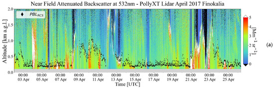
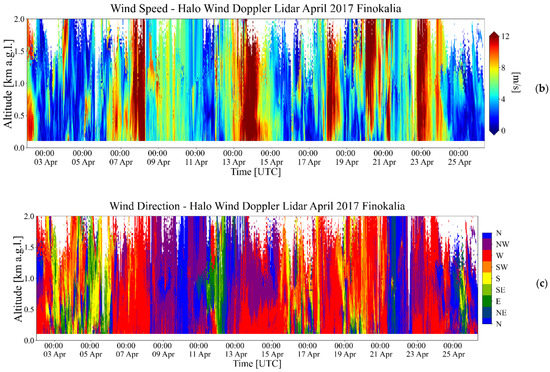
Figure 13.
Period 1-26 April 2017 (a): Attenuated Backscatter Coefficient at 532 nm NF channel of PollyXT Lidar—PBL height retrieved by WCT on RCS (Black Diamonds), Grey color at the bottom of the Figure, identifies the incomplete overlap of PollyXT Lidar for 532 nm NF channel, (b): Wind Speed (m/s) from Halo Wind Doppler Lidar and (c): Wind Direction from Halo Wind Doppler Lidar (Bins in colorbar (0°, 22.5°) (22.5°, 67.5°) (67.5°, 112.5°) (112.5°, 157.5°) (157.5°, 202.5°) (202.5°, 247.5°) (247.5°, 292.5°) (292.5°, 337.5°) (337.5°, 360°)).
Almost 30% of wind measurements of the campaign on the lower levels (105 m) come from W, as shown in the wind rose in Figure 14a. At 525 m, the dominating direction slightly shifts to NW (Figure 14b) and at 1005 m, there is fluctuation of winds from southwestern to northern sector (Figure 14c). This vertical change of wind direction between 105 m and 525 m, is also observed at the second examined case (14 April), where the PBL was very shallow and did not exceed 600 m. The domination of W winds at 105 m and the vertical shift at the first 500 m above ground level, suggests strong layering in the lower levels. More specifically, in Figure 15, the 2-h mean PBL height is calculated for each product: there is no strong daytime evolution and the mean PBL does not exceed 400 m, demonstrating the low layers’ dominance in Finokalia station. During 04:00–08:00 and 16:00–18:00 UTC, MLHTKE present larger variability comparing to the other 2-h averages. PBLRCS and PBLBSC, present the highest deviation at 12:00–14:00 UTC, in addition to the smaller deviations during the rest of the 24 h. The nighttime measured PBL is overestimated by PBLECMWFSEA and underestimated by PBLECMWFLAND, while both overestimate the observed daytime PBL.
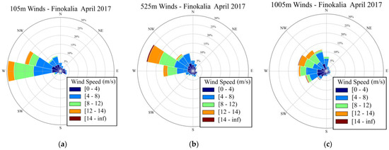
Figure 14.
Wind Rose from Halo Wind Doppler Lidar during 1–26 April 2017 for (a) 105 m level, (b) 525 m level and (c) 1005 m level above ground.
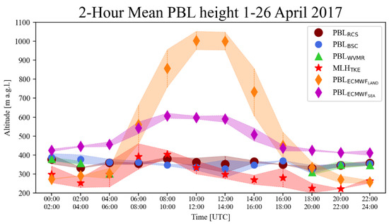
Figure 15.
Mean PBL height calculated every 2 h from WCT on RCS (brown circles), BSC (blue circles), WVMR (green circles), TM on TKEdr (red stars) and ECMWF land bin (orange diamonds) and sea bin (purple diamonds) as described in Figure 8 and Figure 12. Standard deviations are displayed with the same color shading for each product.
Mean Bias Error (MBE), standard deviation (σ) and coefficient of determination (R2) are calculated for the differences between PBL retrievals from different products for 1–26 April 2017 (Figure 16). The absolute value of MBE ranges from 0.2 m to 43.9 m, but only two out of nine comparisons exceed 20 m, which given the resolution of PollyXT (7.5 m) and Halo (30 m) Lidar, can be characterized as reliable MBE. Least-squares regression is used to derive the linear fit between the 15min PBL height estimates. As observed, there is reasonably good correlation PBLWVMR-PBLRCS, PBLBSC-PBLRCS and PBLBSC-PBLWVMR (R2 = 0.92, R2 = 0.92, R2 = 0.9, respectively) for nighttime measurements and PBLBSC-PBLRCS (R2 = 0.93) for daytime measurements during 1–26 April. Cases where TKEdr indicates MLHTKE < 120 m, were replaced with MLHTKE = 60 m, corresponding to half the “lower detection limit” of the instrument, in order to avoid positive or negative biases by excluding or zeroing, respectively. Hence, strong deviations occurred in the comparisons that included PBL retrieved from TKEdr (MLHTKE—PBLBSC, MLHTKE—PBLRCS, MLHTKE—PBLWVMR), with standard deviation exceeding σ = 223. This is expected, given the different nature of direct observations of turbulence and tracers of turbulent mixing as well as previous observations [47]. The systematic difference seen in this inter-comparison, is not attributed to the different methods used but with the different products: WCT is used for the detection of PBL height, using aerosols (RCS, BSC, WVMR) as tracers, while TM is used for the detection of PBL height, using a thermodynamic parameter (TKEdr) as tracer.
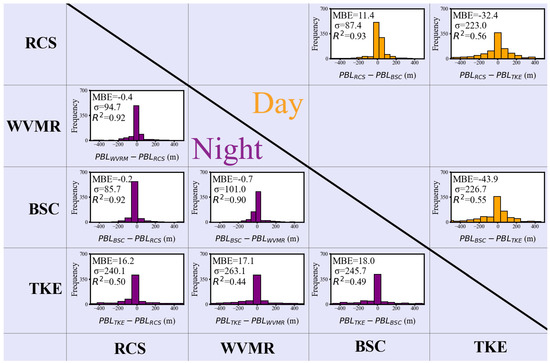
Figure 16.
Statistical analysis of the differences between products and methods for 1–26 April 2017, separated into day and night periods.
In addition to this, the differences of PBLWVMR-PBLRCS (σ = 94.7), PBLBSC-PBLRCS (σ = 85.7), PBLBSC-PBLWVMR (σ = 101) during nighttime and from PBLBSC-PBLRCS (σ = 87.4) during daytime, are described by smaller standard deviation.
4. Conclusions
Finokalia station is placed on a coastal steep cliff, presenting local meteorological characteristics that decisively influence the PBL formation and evolution. Statistical analysis shows that W winds along the coast are dominant in the lower levels most of the time during PreTECT Campaign, forming a shallow PBL that does not present sharp daytime evolution. In addition, when N winds meet the coastline, the forming PBL is clearly higher.
In this study, the cases examined in detail, represent the two different meteorological conditions as described above. It is remarkable that during a sunny day (14 April 2017) the PBL is shallower in comparison to a cloudy one (10 April 2017). The reason for this difference, is that PBL above Finokalia, appears to be dominated by coastal flows rather than thermal convection. More specifically, the strong winds along the coast on a sunny day (14 April), are capping the development of the PBL.
Comparing our observations with the ECMWF results from a sea surface bin and a land surface bin, lead to the conclusion that in both cases, there is an overestimation of the PBL height relative to the estimates derived from lidar, with the exception of nighttime hours (00:00–06:00, 18:00–24:00 UTC), where the land bin underestimates the observed PBL. A coastal region with complex topography such as Finokalia, where convection plays a much smaller role in PBL evolution, favors the formation of a PBL that is not well described by the relatively coarse scale model. The model-measurements differences are addressed to the influence of changes in surface roughness in combination with the horizontal advection of air across this discontinuity. This also emphasizes the importance of the actual PBL measurements when the models are uncertain in such regions.
Overall, the WCT method applied on RCS, WVMR, and BSC, is a trustworthy reference for the detection of layering. The synergistic use of these products is crucial for the determination of PBL height. WVMR is a considerable tracer for the boundary layer dynamics, since it is strongly related to wind transport. Especially in coastal areas, the effect of water surfaces on the evolution of PBL is very well recorded when considering water vapor profiles. RCS and BSC are proportional to the aerosol concentration and constitute a reliable indicator for layering detection. However, different tracers for PBL, may lead to distinct results, but contribute to building a more accurate image of the boundary layer diurnal evolution. Applying TM on TKEdr profiles, captures the well-mixed layers with thermal and mechanical turbulence, whereas WCT captures a less turbulent layer that contains aerosols (case 10 April 2017 18:00–24:00 UTC). Thus, care must be taken in interpreting the tracer-based PBL height, as the captured layer can differ from the nocturnal layer or the MLH.
In some cases, the mesoscale circulation that causes the strong winds in the Aegean Sea, superimposes on the mean wind flow in Finokalia, and probably resembles a sea-breeze-type circulation. At the end of the day, wind speed and direction change and probably relate to land-breeze-type circulation. These conditions favor the development of a TIBL, stable during nighttime, mainly represented by MLHTKE.
A possible future research study, could be the creation of an automated algorithm that retrieves the PBL height in Finokalia, given an established pattern of the winds interfering with the PBL height behavior and the development of an IBL.
Author Contributions
Conceptualization, I.T., V.A. and E.M.; methodology, I.T., E.M. and V.V.; software, I.T.; validation, I.T., E.M., V.V., V.A., M.T. (Maria Tombrou) and I.P.R.; formal analysis, I.T., E.M., V.V. and I.P.R.; investigation, I.T., E.M., V.V., V.A., I.P.R., A.G., M.T. (Maria Tombrou), M.K., E.G. and H.F.; resources, V.A., E.M., A.G. and N.M.; data curation, I.T., A.G., E.M., V.V., A.K., V.D., M.K. and M.T. (Maria Tsichla); writing—original draft preparation, I.T. and I.P.R.; writing—review and editing, I.T., V.V., E.M. and M.T. (Maria Tombrou); visualization, I.T., A.G., A.K. and E.M.; supervision, V.A., M.T. (Maria Tombrou) and E.G.; project administration V.A. and E.M.; funding acquisition, V.A. All authors have read and agreed to the published version of the manuscript.
Funding
This research was funded by the project “PANhellenic infrastructure for Atmospheric Composition and climatE change” (no. MIS 5021516), which is implemented under the action “Reinforcement of the Research and Innovation Infrastructure”, funded by the “Competitiveness, Entrepreneurship and Innovation” Operational Programme (NSRF 2014–2020) and co-financed by Greece and the European Union (European Regional Development Fund). Support was also provided by D-TECT (Grant Agreement 725698) funded by the European Research Council (ERC) under the European Union’s Horizon 2020 research and innovation program. We thank the ACTRIS-2 and ACTRIS preparatory phase projects that have received funding from the European Union’s Horizon 2020 Framework Program for Research and Innovation (grant agreement no. 654109) and from European Union’s Horizon 2020 Coordination and Support Action (grant agreement no. 739530), respectively. Finally, the research was also funded by “Stavros Niarchos Foundation” (SNF).
Data Availability Statement
The PollyXT data used are publicly available as quicklooks in the PollyNET website (polly.tropos.de, accessed on 17 Auguste 2022) and available upon request from E.M. and V.A. The Halo Wind Doppler Lidar Data are available as quicklooks in the PreTECT Campaign Website (http://PRE-TECT.space.noa.gr/ (accessed on 15 August 2022)).
Acknowledgments
The authors would like to acknowledge ACTRIS [48] and for the data collection, calibration, processing and dissemination. We thank the PRETECT team for providing access to the PRE-TECT datasets [27]. NOA Team acknowledges the support of Stavros Niarchos Foundatio (SNF).
Conflicts of Interest
The authors declare no conflict of interest.
Abbreviations
The following abbreviations are used in this manuscript:
| PBL | Planetary Boundary Layer |
| IBL | Internal Boundary Layer |
| TIBL | Thermal Internal Boundary Layer |
| WCT | Wavelet Covariance Transform |
| TM | Threshold Method |
| RCS | Range Corrected Signal |
| NF | Near Field |
| BSC | Backscatter Coefficient |
| WVMR | Water Vapor Mixing Ratio |
| TKEdr | Turbulent Kinetic Energy dissipation rate |
| PBLRCS | Planetary Boundary Layer height retrieved from WCT on RCS from 532nm NF channel of PollyXT Lidar |
| PBLWVMR | Planetary Boundary Layer height retrieved from WCT on WVMR of PollyXT Lidar |
| PBLBSC | Planetary Boundary Layer height retrieved from WCT on BSC of Halo Wind Lidar |
| MLHTKE | Mixing Layer Height retrieved from TM on TKEdr of Halo Wind Lidar |
| MLH | Mixing layer Height |
| MBE | Mean Bias Error |
| N, E, S, W | North (0°/360°), East (90°), South (180°), West (270°) |
| PBLECMWFSEA | PBL height from ECMWF bin above sea |
| PBLECMWFLAND | PBL height from ECMWF bin above land |
References
- Stull, R.B. An Introduction to Boundary Layer Meteorology; Springer: Berlin/Heidelberg, Germany, 1988; pp. 2–21. [Google Scholar] [CrossRef]
- Wei, J.; Tang, G.; Zhu, X.; Wang, L.; Liu, Z.; Cheng, M.; Münkel, C.; Li, X.; Wang, Y. Thermal internal boundary layer and its effects on air pollutants during summer in a coastal city in North China. J. Environ. Sci. 2018, 70, 37–44. [Google Scholar] [CrossRef] [PubMed]
- Garratt, J.R.; Ryan, B.F. The Structure of the Stably Stratified Internal Boundary Layer in Offshore Flow over the Sea. In Boundary Layer Studies and Applications; Springer: Berlin/Heidelberg, Germany, 1989; pp. 17–40. [Google Scholar] [CrossRef]
- Garratt, J.R. The stably stratified internal boundary layer for steady and diurnally varying offshore flow. Bound. Layer Meteorol. 1987, 38, 369–394. [Google Scholar] [CrossRef]
- Gerasopoulos, E.; Amiridis, V.; Kazadzis, S.; Kokkalis, P.; Eleftheratos, K.; Andreae, M.O.; Andreae, T.W.; El-Askary, H.; Zerefos, C.S. Three-year ground based measurements of aerosol optical depth over the Eastern Mediterranean: The urban environment of Athens. Atmos. Chem. Phys. 2011, 11, 2145–2159. [Google Scholar] [CrossRef]
- Bossioli, E.; Tombrou, M.; Kalogiros, J.; Allan, J.; Bacak, A.; Bezantakos, S.; Biskos, G.; Coe, H.; Jones, B.T.; Kouvarakis, G.; et al. Atmospheric composition in the Eastern Mediterranean: Influence of biomass burning during summertime using the WRF-Chem model. Atmos. Environ. 2016, 132, 317–331. [Google Scholar] [CrossRef]
- Jacobeit, J. Variations of trough positions and precipitation patterns in the mediterranean area. J. Climatol. 1987, 7, 453–476. [Google Scholar] [CrossRef]
- Lionello, P.; Galati, M.B. Links of the significant wave height distribution in the Mediterranean Sea with the Northern Hemisphere teleconnection patterns. Adv. Geosci. 2008, 17, 13–18. [Google Scholar] [CrossRef]
- Miglietta, M.M.; Moscatello, A.; Conte, D.; Mannarini, G.; Lacorata, G.; Rotunno, R. Numerical analysis of a Mediterranean ‘hurricane’ over south-eastern Italy: Sensitivity experiments to sea surface temperature. Atmos. Res. 2011, 101, 412–426. [Google Scholar] [CrossRef]
- Marinou, E.; Voudouri, K.A.; Tsikoudi, I.; Drakaki, E.; Tsekeri, A.; Rosoldi, M.; Ene, D.; Baars, H.; O’Connor, E.; Amiridis, V.; et al. Geometrical and Microphysical Properties of Clouds Formed in the Presence of Dust above the Eastern Mediterranean. Remote Sens. 2021, 13, 5001. [Google Scholar] [CrossRef]
- Tombrou, M.; Bossioli, E.; Kalogiros, J.; Allan, J.D.; Bacak, A.; Biskos, G.; Coe, H.; Dandou, A.; Kouvarakis, G.; Mihalopoulos, N.; et al. Physical and chemical processes of air masses in the Aegean Sea during Etesians: Aegean-GAME airborne campaign. Sci. Total Environ. 2015, 506–507, 201–216. [Google Scholar] [CrossRef]
- Hoerling, M.; Eischeid, J.; Perlwitz, J.; Quan, X.; Zhang, T.; Pegion, P. On the increased frequency of Mediterranean drought. J. Clim. 2012, 25, 2146–2161. [Google Scholar] [CrossRef]
- Barros, V.; Field, C.; Dokken, D.; Mastrandrea, M.; Mach, K.; Bilir, T.; Chatterjee, M.; Ebi, K.; Estrada, Y.; Genova, R.; et al. Part B: Regional Aspects. Contribution of Working Group II to the Fifth Assessment Report of the Intergovernmental Panel on Climate Change. In IPCC, 2014: Impacts, Adaptation, and Vulnerability; Cambridge University Press: Cambridge, UK, 2004. [Google Scholar]
- Solomos, S.; Ansmann, A.; Mamouri, R.-E.; Binietoglou, I.; Patlakas, P.; Marinou, E.; Amiridis, V. Remote sensing and modelling analysis of the extreme dust storm hitting the Middle East and eastern Mediterranean in September 2015. Atmos. Chem. Phys. 2017, 17, 4063–4079. [Google Scholar] [CrossRef]
- Baars, H.; Ansmann, A.; Engelmann, R.; Althausen, D. Continuous monitoring of the boundary-layer top with lidar. Atmos. Chem. Phys. 2008, 8, 7281–7296. [Google Scholar] [CrossRef]
- Kokkalis, P.; Alexiou, D.; Papayannis, A.; Rocadenbosch, F.; Soupiona, O.; Raptis, P.I.; Mylonaki, M.; Tzanis, C.G.; Christodoulakis, J. Application and Testing of the Extended-Kalman-Filtering Technique for Determining the Planetary Boundary-Layer Height over Athens, Greece. Bound. Layer Meteorol. 2020, 176, 125–147. [Google Scholar] [CrossRef]
- Granados-Muñoz, M.J.; Navas-Guzmán, F.; Bravo-Aranda, J.A.; Guerrero-Rascado, J.L.; Lyamani, H.; Fernández-Gálvez, J.; Alados-Arboledas, L. Automatic determination of the planetary boundary layer height using lidar: One-yearanalysis over southeastern Spain. J. Geophys. Res. 2012, 117, D18208. [Google Scholar] [CrossRef]
- Zhang, M.; Tian, P.; Zeng, H.; Wang, L.; Liang, J.; Cao, X.; Zhang, L. A Comparison of Wintertime Atmospheric Boundary Layer Heights Determined by Tethered Balloon Soundings and Lidar at the Site of SACOL. Remote Sens. 2021, 13, 1781. [Google Scholar] [CrossRef]
- Dang, R.; Yang, Y.; Hu, X.-M.; Wang, Z.; Zhang, S. A Review of Techniques for Diagnosing the Atmospheric Boundary Layer Height (ABLH) Using Aerosol Lidar Data. Remote Sens. 2019, 11, 1590. [Google Scholar] [CrossRef]
- Kim, M.-H.; Yeo, H.; Park, S.; Park, D.-H.; Omar, A.; Nishizawa, T.; Shimizu, A.; Kim, S.-W. Assessing CALIOP-Derived Planetary Boundary Layer Height Using Ground-Based Lidar. Remote Sens. 2021, 13, 1496. [Google Scholar] [CrossRef]
- Vakkari, V.; O’Connor, E.J.; Nisantzi, A.; Mamouri, R.E.; Hadjimitsis, D.G. Low-level mixing height detection in coastal locations with a scanning Doppler lidar. Atmos. Meas. Tech. 2015, 8, 1875–1885. [Google Scholar] [CrossRef]
- Amiridis, V.; Melas, D.; Balis, D.S.; Papayannis, A.; Founda, D.; Katragkou, E.; Giannakaki, E.; Mamouri, R.E.; Gerasopoulos, E.; Zerefos, C. Aerosol Lidar observations and model calculations of the Planetary Boundary Layer evolution over Greece, during the March 2006 Total Solar Eclipse. Atmos. Chem. Phys. 2007, 7, 6181–6189. [Google Scholar] [CrossRef]
- Tsaknakis, G.; Papayannis, A.; Kokkalis, P.; Amiridis, V.; Kambezidis, H.D.; Mamouri, R.E.; Georgoussis, G.; Avdikos, G. Inter-comparison of lidar and ceilometer retrievals for aerosol and Planetary Boundary Layer profiling over Athens, Greece. Atmos. Meas. Tech. 2011, 4, 1261–1273. [Google Scholar] [CrossRef]
- Tombrou, M.; Dandou, A.; Helmis, C.; Akylas, E.; Angelopoulos, G.; Flocas, H.; Assimakopoulos, V.; Soulakellis, N. Model evaluation of the atmospheric boundary layer and mixed-layer evolution. Bound. Layer Meteorol. 2007, 124, 61–79. [Google Scholar] [CrossRef]
- Dandou, A.; Tombrou, M.; Schäfer, K.; Emeis, S.; Protonotariou, A.P.; Bossioli, E.; Soulakellis, N.; Suppan, P. A Comparison between Modelled and Measured Mixing-Layer Height over Munich. Bound. Layer Meteorol. 2009, 131, 425–440. [Google Scholar] [CrossRef]
- Dandou, A.; Tombrou, M.; Kalogiros, J.; Bossioli, E.; Biskos, G.; Mihalopoulos, N.; Coe, H. Investigation of Turbulence Parametrization Schemes with Reference to the Atmospheric Boundary Layer over the Aegean Sea during Etesian Winds. Bound. Layer Meteorol. 2017, 164, 303–329. [Google Scholar] [CrossRef]
- The PRE-TECT Experimental Campaign. Available online: http://PRE-TECT.space.noa.gr/ (accessed on 15 August 2022).
- Engelmann, R.; Kanitz, T.; Baars, H.; Heese, B.; Althausen, D.; Skupin, A.; Wandinger, U.; Komppula, M.; Stachlewska, I.S.; Amiridis, V.; et al. The automated multiwavelength Raman polarization and water-vapor lidar PollyXT: The neXT generation. Atmos. Meas. Tech. 2016, 9, 1767–1784. [Google Scholar] [CrossRef]
- Pearson, G.; Davies, F.; Collier, C. An Analysis of the Performance of the UFAM Pulsed Doppler Lidar for Observing the Boundary Layer. J. Atmos. Ocean. Technol. 2009, 26, 240–250. [Google Scholar] [CrossRef]
- Manninen, A.J.; O’Connor, E.J.; Vakkari, V.; Petäjä, T. A generalised background correction algorithm for a Halo Doppler lidar and its application to data from Finland. Atmos. Meas. Tech. 2016, 9, 817–827. [Google Scholar] [CrossRef]
- Whiteman, D.N.; Melfi, S.H.; Ferrare, R.A. Raman lidar system for the measurement of water vapor and aerosols in the Earth’s atmosphere. Appl. Opt. 1992, 31, 3068–3082. [Google Scholar] [CrossRef]
- Dai, G.; Althausen, D.; Hofer, J.; Engelmann, R.; Seifert, P.; Bühl, J.; Mamouri, R.-E.; Wu, S.; Ansmann, A. Calibration of Raman lidar water vapor profiles by means of AERONET photometer observations and GDAS meteorological data. Atmos. Meas. Tech. 2018, 11, 2735–2748. [Google Scholar] [CrossRef]
- Foth, A.; Baars, H.; Di Girolamo, P.; Pospichal, B. Water vapour profiles from Raman lidar automatically calibrated by microwave radiometer data during HOPE. Atmos. Chem. Phys. 2015, 15, 7753–7763. [Google Scholar] [CrossRef]
- Manninen, A.J.; Marke, T.; Tuononen, M.J.; O’Connor, E.J. Atmospheric boundary layer classification with Doppler lidar. J. Geophys. Res. Atmos. 2018, 123, 8172–8189. [Google Scholar] [CrossRef]
- Vakkari, V.; Manninen, A.J.; O’Connor, E.J.; Schween, J.H.; van Zyl, P.G.; Marinou, E. A novel post-processing algorithm for Halo Doppler lidars. Atmos. Meas. Tech. 2019, 12, 839–852. [Google Scholar] [CrossRef]
- Browning, K.A.; Wexler, R. The Determination of Kinematic Properties of a Wind Field Using Doppler Radar. J. Appl. Meteorol. Climatol. 1968, 7, 105–113. [Google Scholar] [CrossRef]
- O’Connor, E.J.; Illingworth, A.J.; Brooks, I.M.; Westbrook, C.D.; Hogan, R.J.; Davies, F.; Brooks, B.J. A Method for Estimating the Turbulent Kinetic Energy Dissipation Rate from a Vertically Pointing Doppler Lidar, and Independent Evaluation from Balloon-Borne In Situ Measurements. J. Atmos. Ocean. Technol. 2010, 27, 1652–1664. [Google Scholar] [CrossRef]
- ECMWF ERA5 Information. Available online: https://www.ecmwf.int/en/forecasts/dataset/ecmwf-reanalysis-v5 (accessed on 15 August 2022).
- ECMWF L137 Model Level Definitions. Available online: https://confluence.ecmwf.int/display/udoc/L137+model+level+definitions (accessed on 15 August 2022).
- Vogelezang, D.H.P.; Holtslag, A.A.M. Evaluation and model impacts of alternative boundary-layer height formulations. Bound. Layer Meteorol. 1996, 81, 245–269. [Google Scholar] [CrossRef]
- Copernicus Climate Data Store (CDS). Available online: https://cds.climate.copernicus.eu/ (accessed on 15 August 2022).
- Skamarock, W.C.; Klemp, J.B.; Dudhia, J.; Gill, D.O.; Zhiquan, L.; Berner, J.; Wang, W.; Powers, J.G.; Duda, M.G.; Barker, D.M.; et al. A Description of the Advanced Research WRF Model Version 4; NCAR Technial Note NCAR/TN-475+STR; NCAR: Boulder, CO, USA, 2019; p. 145. [Google Scholar]
- Stohl, A.; Forster, C.; Frank, A.; Seibert, P.; Wotawa, G. Technical note: The Lagrangian particle dispersion model FLEXPART version 6.2. Atmos. Chem. Phys. 2005, 5, 2461–2474. [Google Scholar] [CrossRef]
- Pisso, I.; Sollum, E.; Grythe, H.; Kristiansen, N.I.; Cassiani, M.; Eckhardt, S.; Arnold, D.; Morton, D.; Thompson, R.L.; Groot Zwaaftink, C.D.; et al. FLEXPART 10.4 (Version 10.4). Geosci. Model Dev. Discuss. Zenodo 2019, 12, 1–43. [Google Scholar] [CrossRef]
- Stohl, A.; Prata, A.J.; Eckhardt, S.; Clarisse, L.; Durant, A.; Henne, S.; Kristiansen, N.I.; Minikin, A.; Schumann, U.; Seibert, P.; et al. Determination of time- and height-resolved volcanic ash emissions and 20 their use for quantitative ash dispersion modeling: The 2010 Eyjafjallajökull eruption. Atmos. Chem. Phys. 2011, 11, 4333–4351. [Google Scholar] [CrossRef]
- Brooks, I.M. Finding Boundary Layer Top: Application of a Wavelet Covariance Transform to Lidar Backscatter Profiles. J. Atmos. Ocean. Technol. 2003, 20, 1092–1105. [Google Scholar] [CrossRef]
- Schween, J.H.; Hirsikko, A.; Löhnert, U.; Crewell, S. Mixing-layer height retrieval with ceilometer and Doppler lidar: From case studies to long-term assessment. Atmos. Meas. Tech. 2014, 7, 3685–3704. [Google Scholar] [CrossRef]
- ACTRIS, The Aerosol, Clouds and Trace Gases Research Infrastructure. Available online: https://www.actris.eu (accessed on 15 August 2022).
Publisher’s Note: MDPI stays neutral with regard to jurisdictional claims in published maps and institutional affiliations. |
© 2022 by the authors. Licensee MDPI, Basel, Switzerland. This article is an open access article distributed under the terms and conditions of the Creative Commons Attribution (CC BY) license (https://creativecommons.org/licenses/by/4.0/).