

Sen2Like: Paving the Way towards Harmonization and Fusion of Optical Data

 , ,
, ,  ,
,  , , , ,
Abstract
:1. Introduction
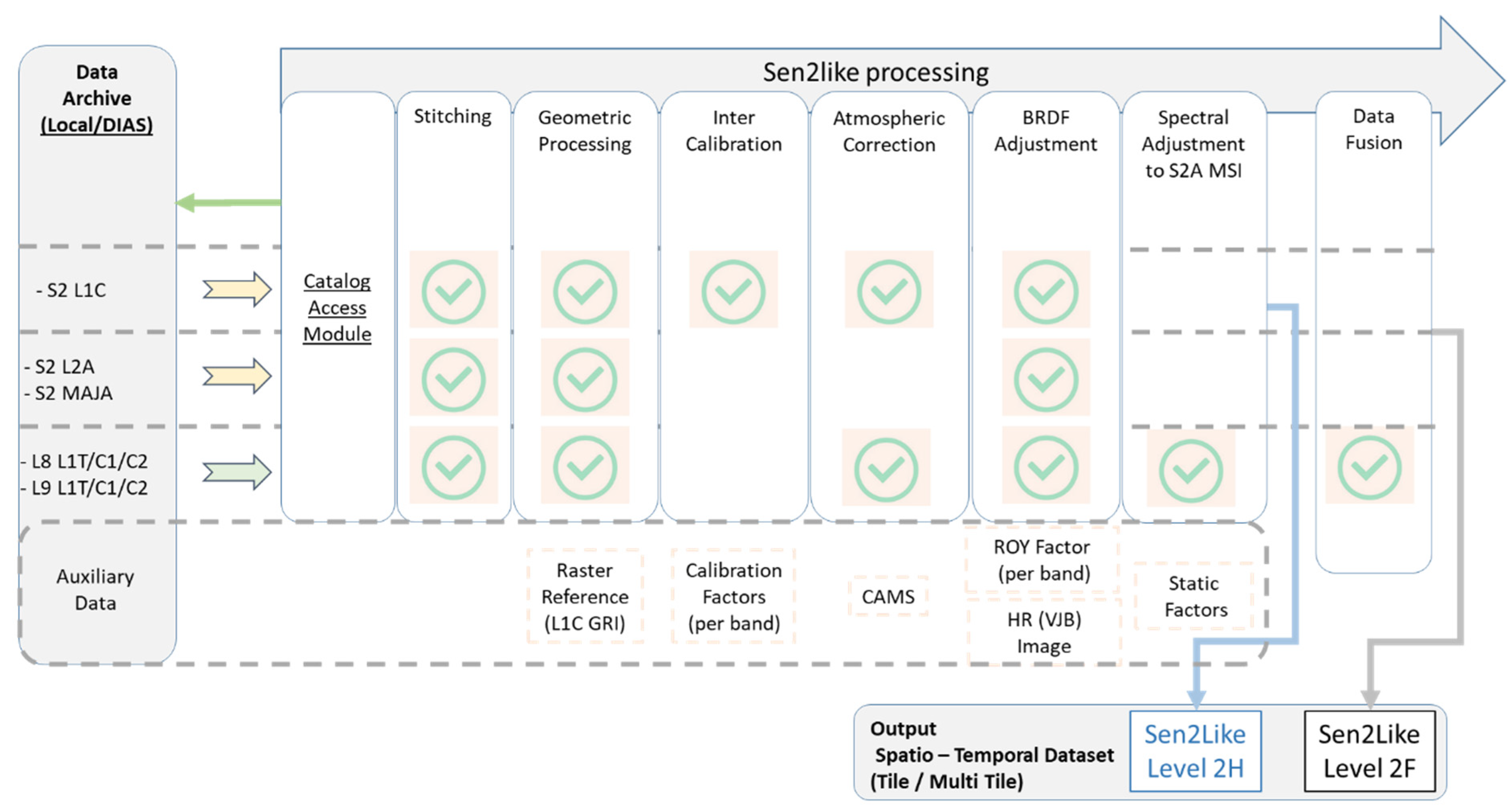
2. Materials and Methods
- i.
- Image stitching of the different tiles;
- ii.
- Geometric corrections including the co-registration to a reference image;
- iii.
- Inter-calibration (for S2 L1C);
- iv.
- Atmospheric corrections;
- v.
- Transformation to Nadir Bidirectional Reflectance Distribution Function (BRDF) Adjusted Reflectance (NBAR);
- vi.
- Application of Spectral Band Adjustment Factor (SBAF) (for LS8/9);
- vii.
- Production of LS8/LS9 high resolution 10 m pixel spacing data (data fusion).
2.1. Sen2Like Software Design Elements
2.2. Product Description and Auxiliary Data
- The geometric reference data involved in the co-registration step;
- The Copernicus Atmosphere Monitoring Service (CAMS) data [21], meteorological data released by the European Centre for Medium-Range Weather Forecasts (ECMWF);
- The spectral adjustment parameter set (SBAF corrections);
- The calibration processing coefficient;
- The directional effects correction factors (NBAR corrections).
2.3. Image Correction Methodology
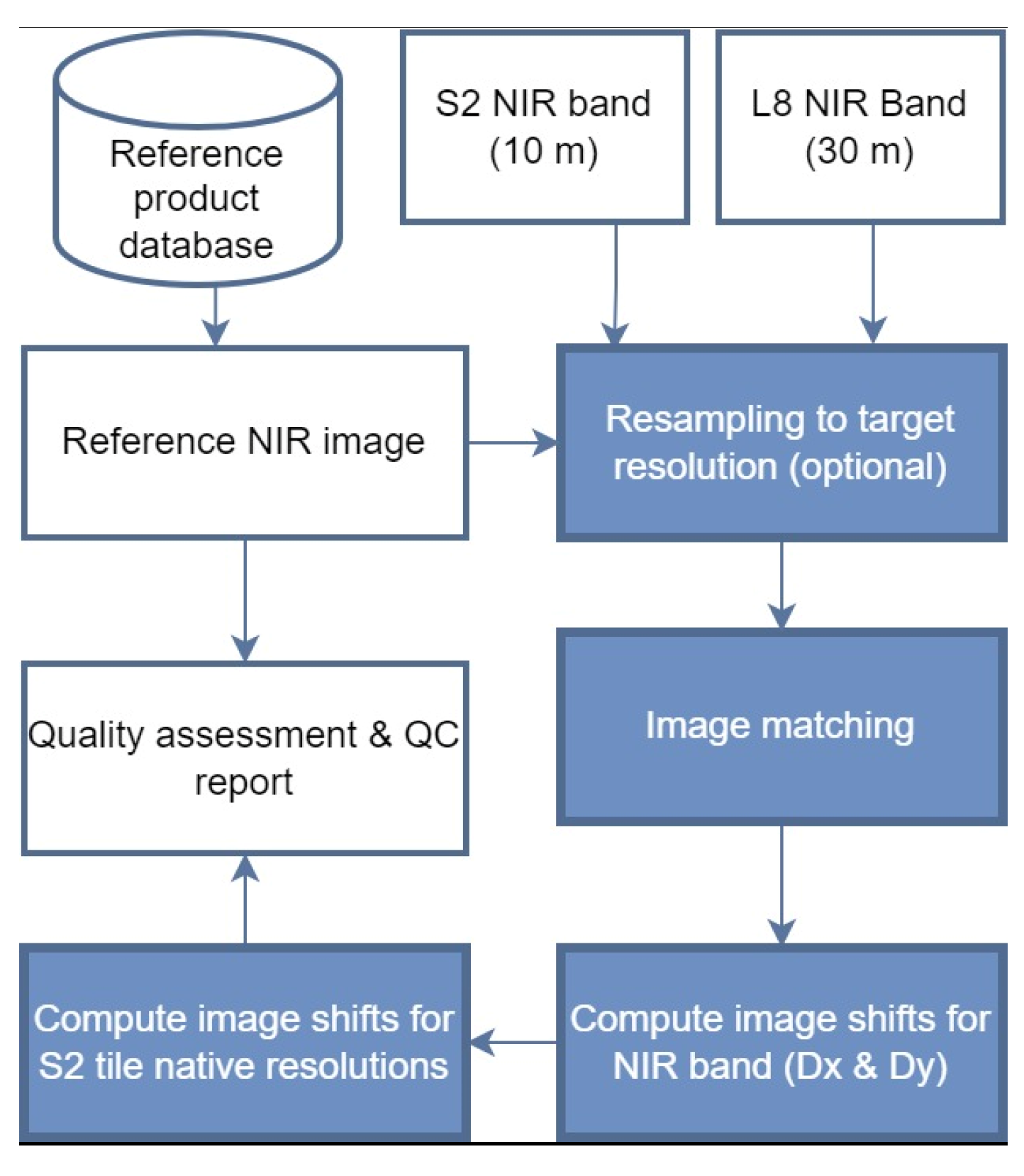
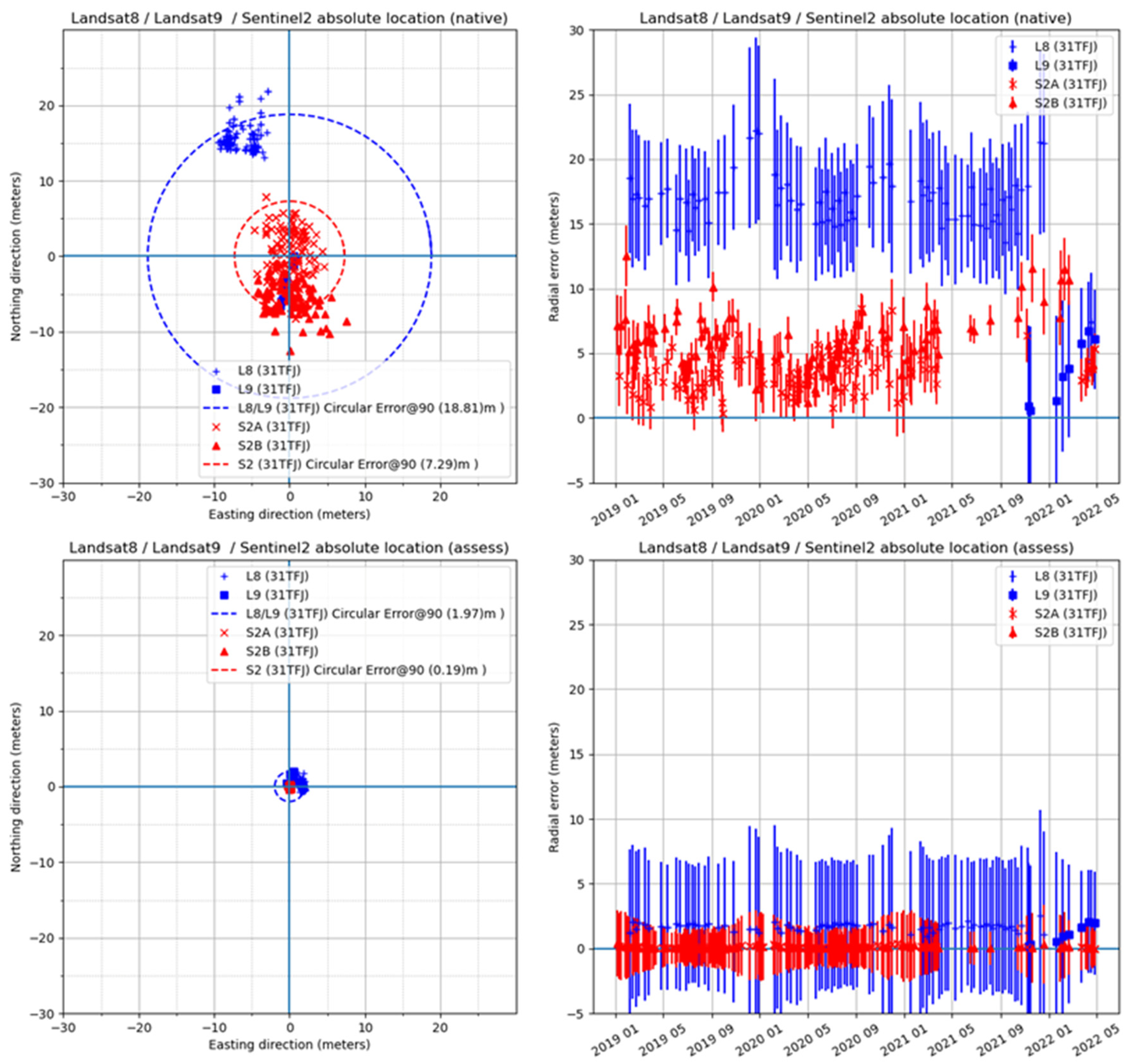
2.3.1. Geometric Correction
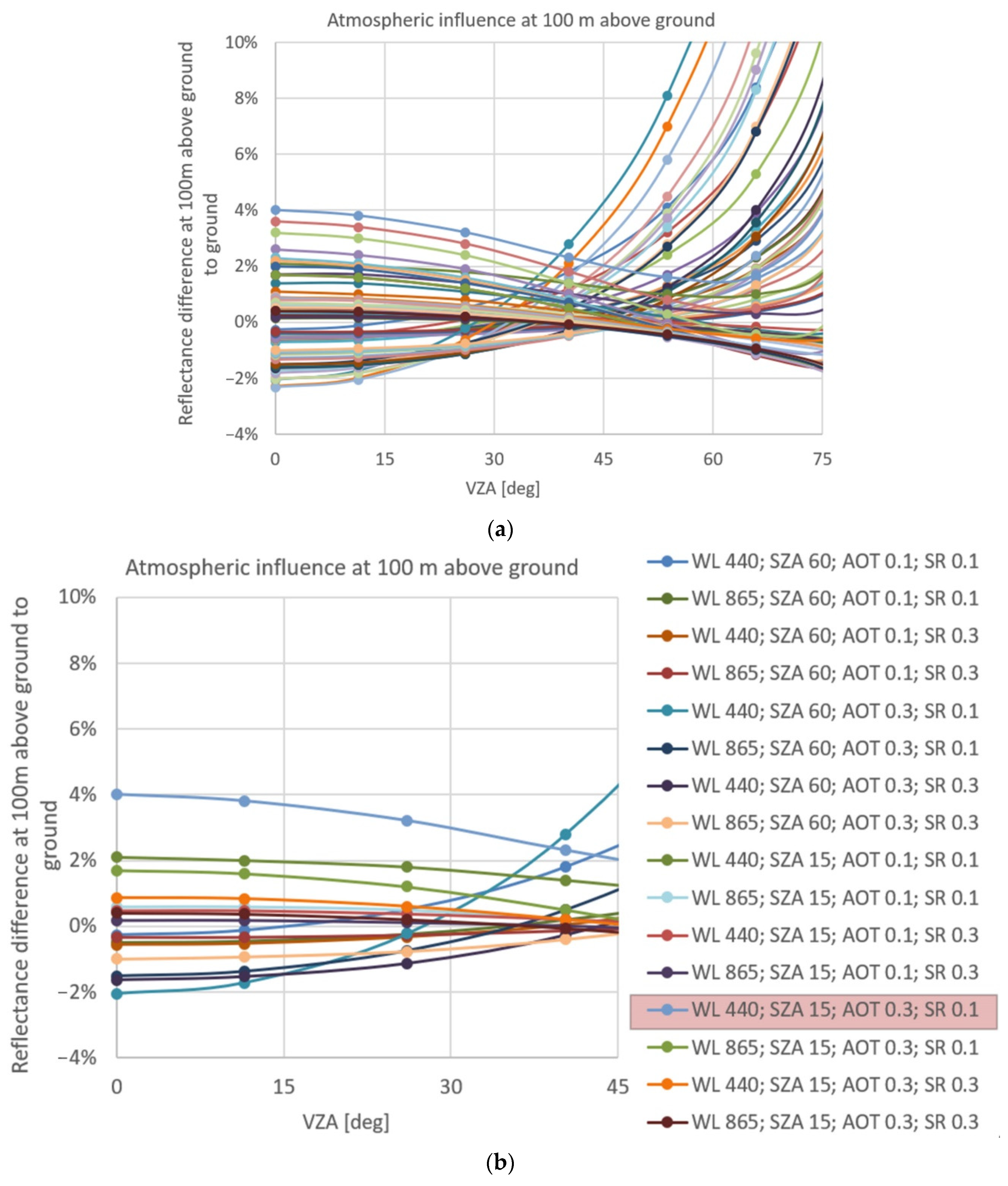
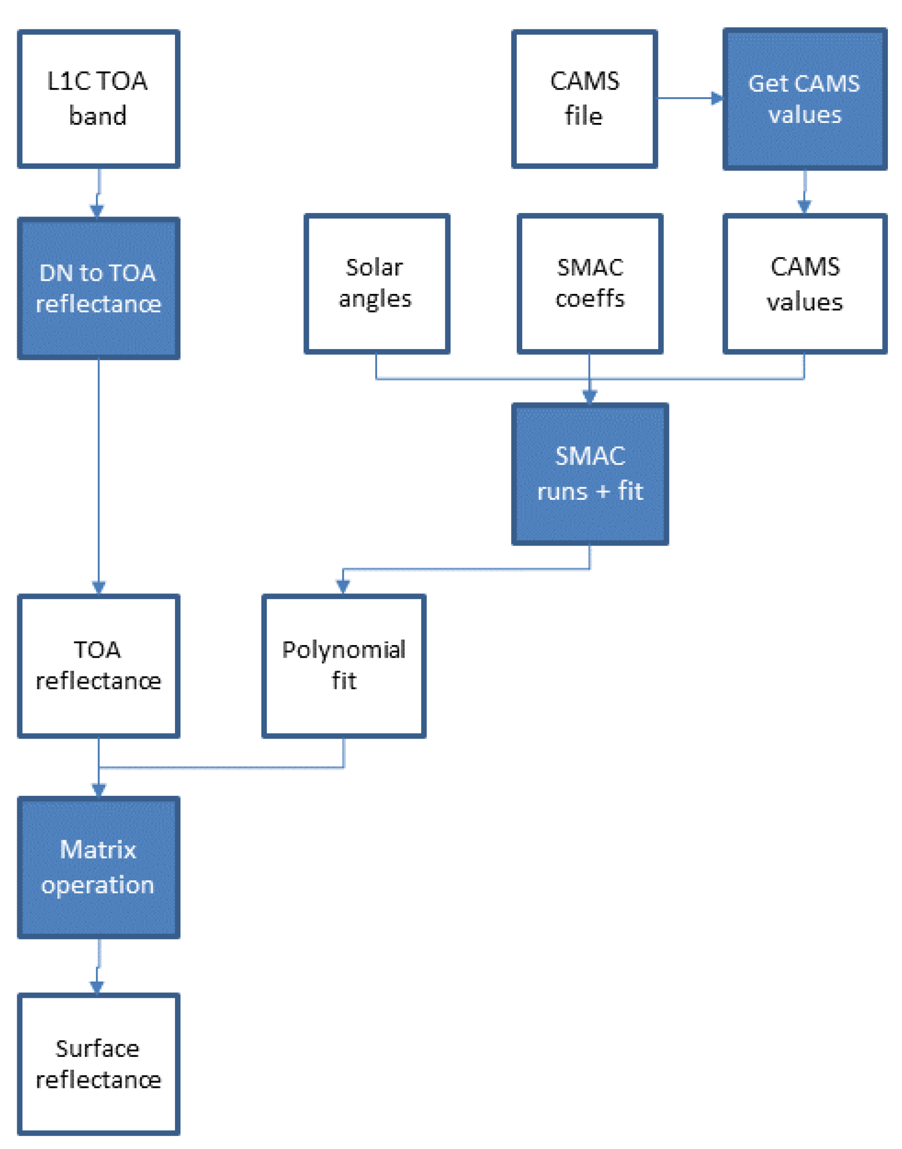
2.3.2. Atmospheric Correction
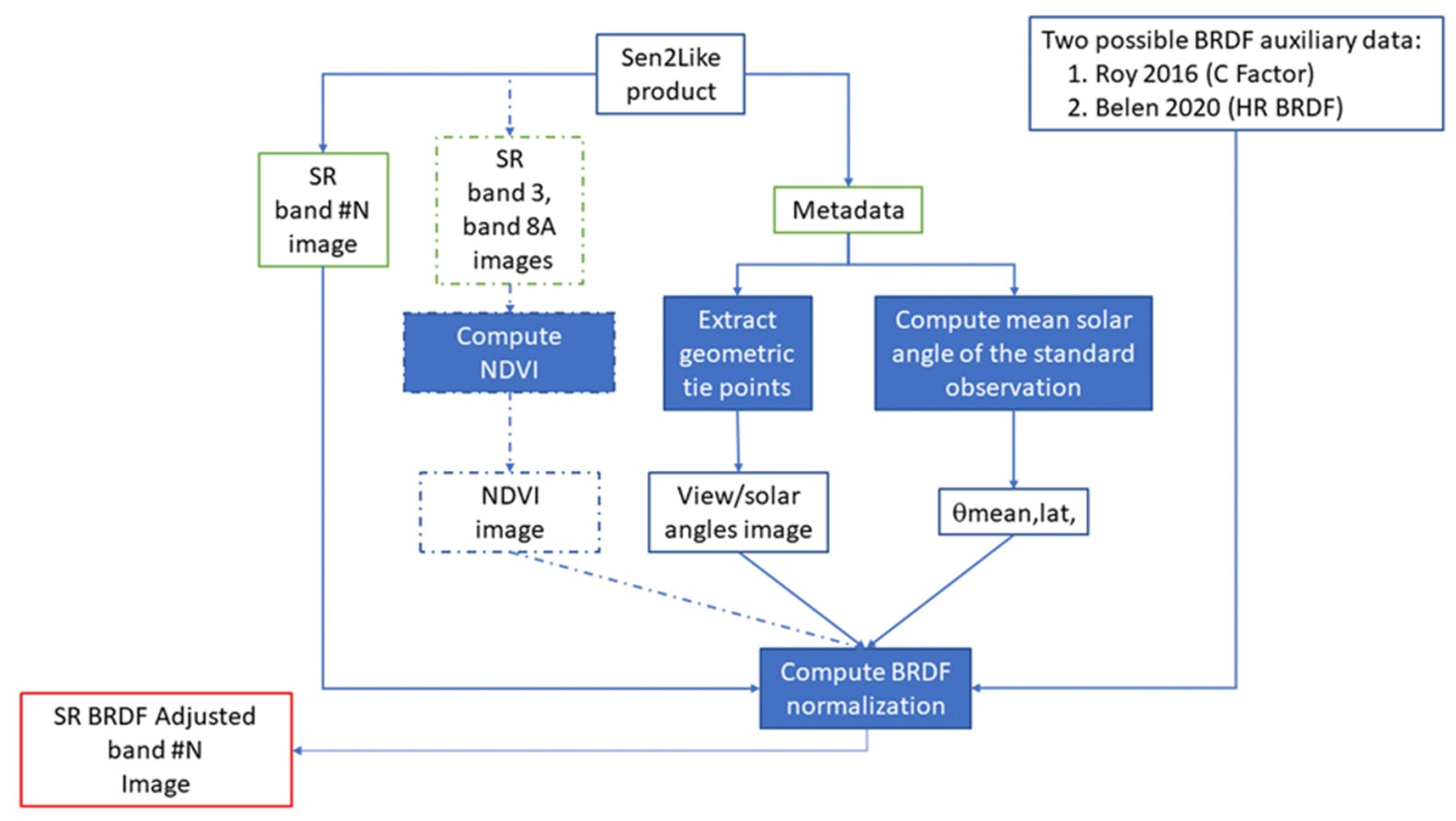
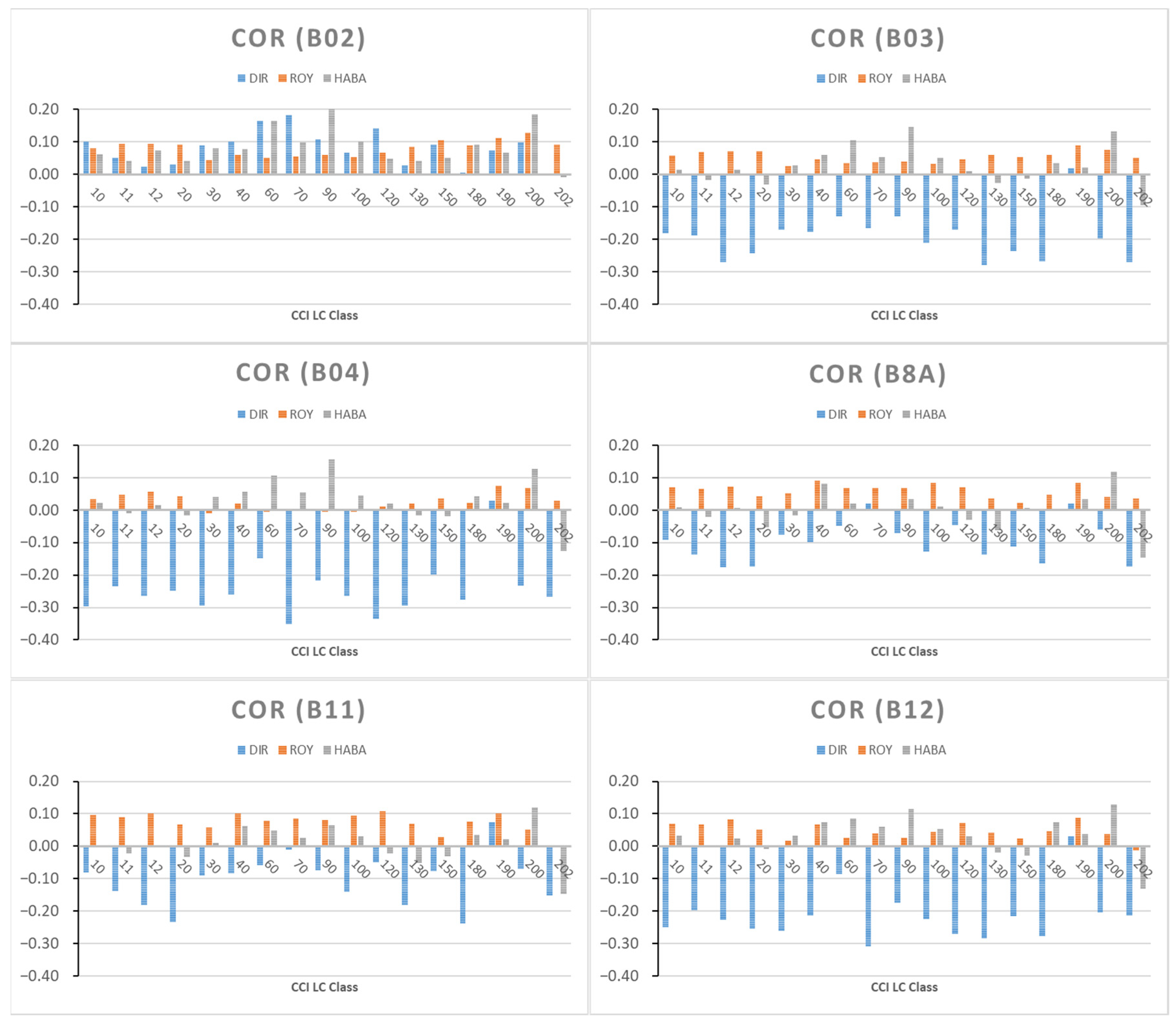
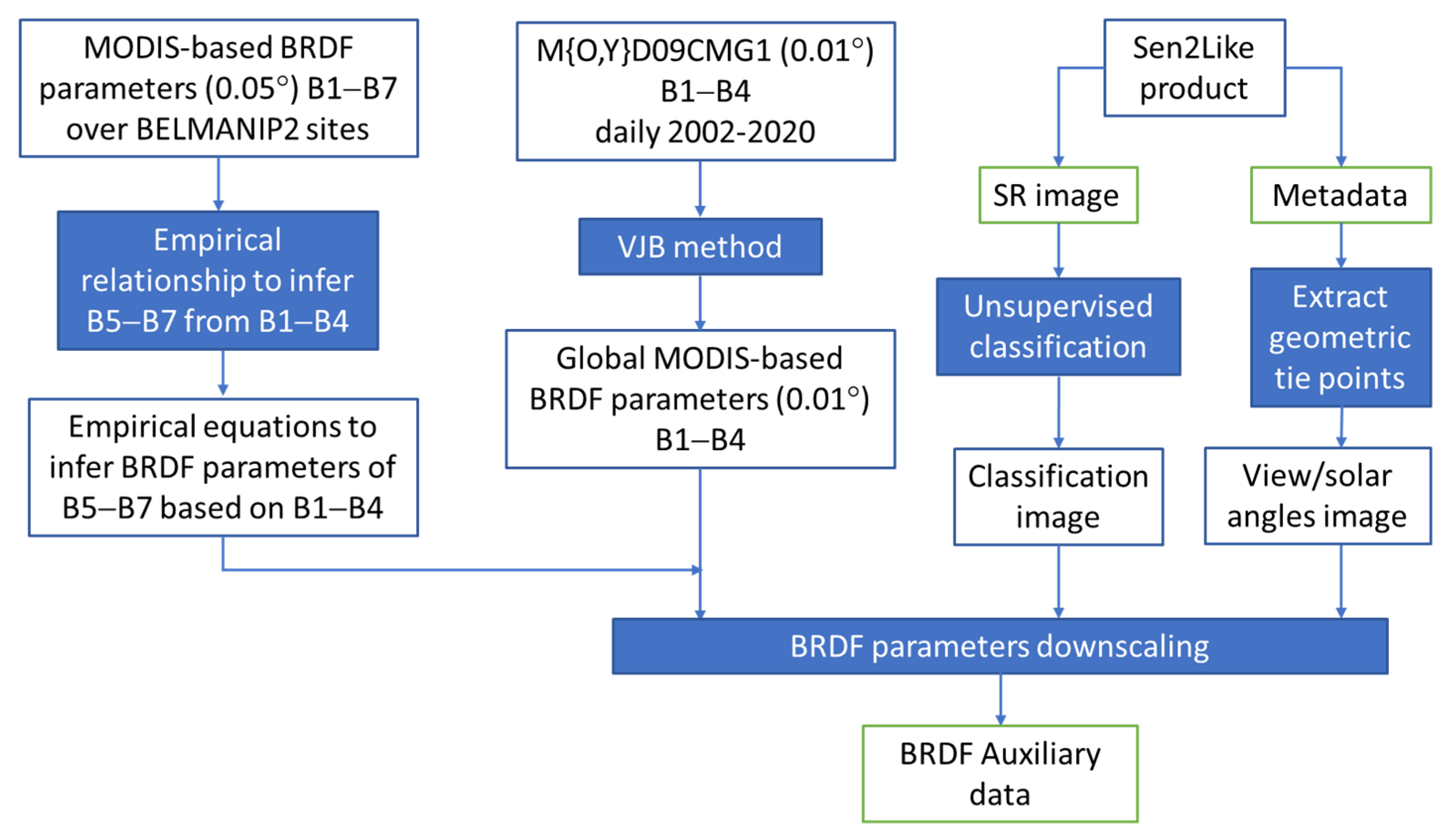
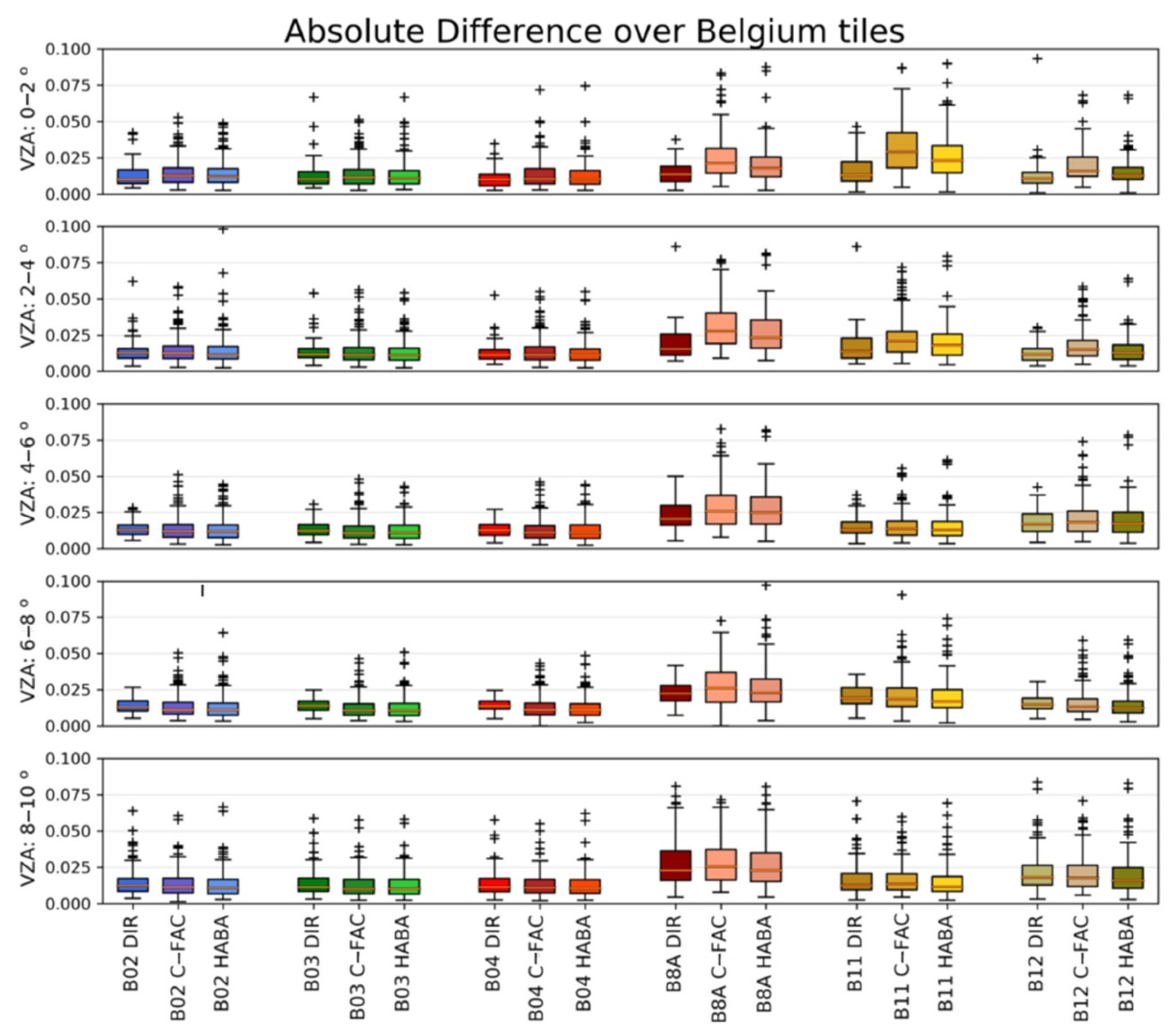
2.3.3. BRDF Correction
- and are the volume and the roughness parameters that describe the BRDF shape,
- The parameters are the solar/viewing, zenith and the relative azimuth,
- The parameter is related to the spectral band taken into consideration for this calculation.
- are six-degree polynomial coefficients—the parameter values are listed in Table 3,
- is the latitude of the MGRS tile scene center.
2.3.4. Spectral Band Adjustment Factor (SBAF)
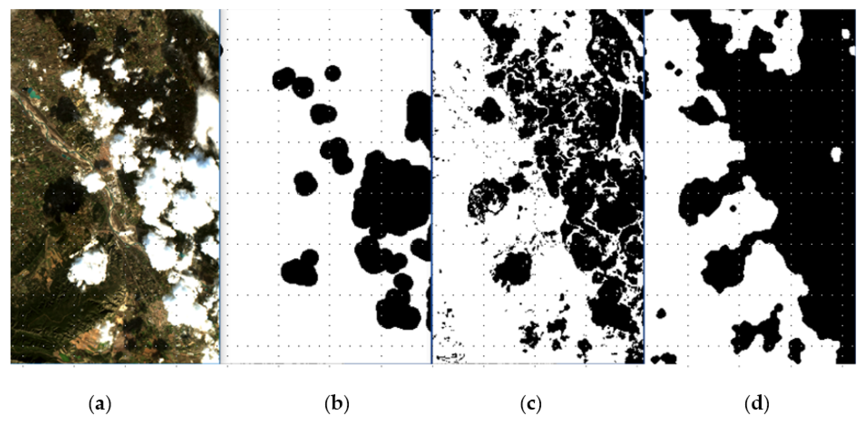
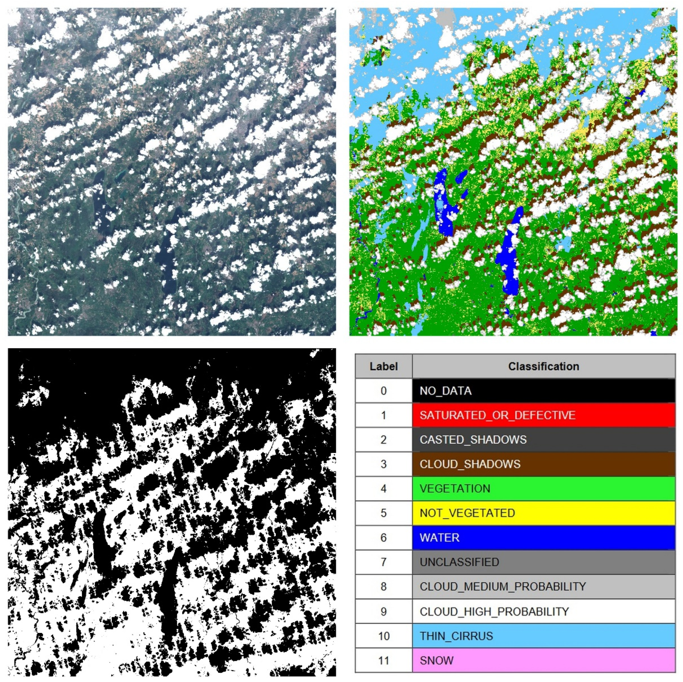
2.4. Validity Mask
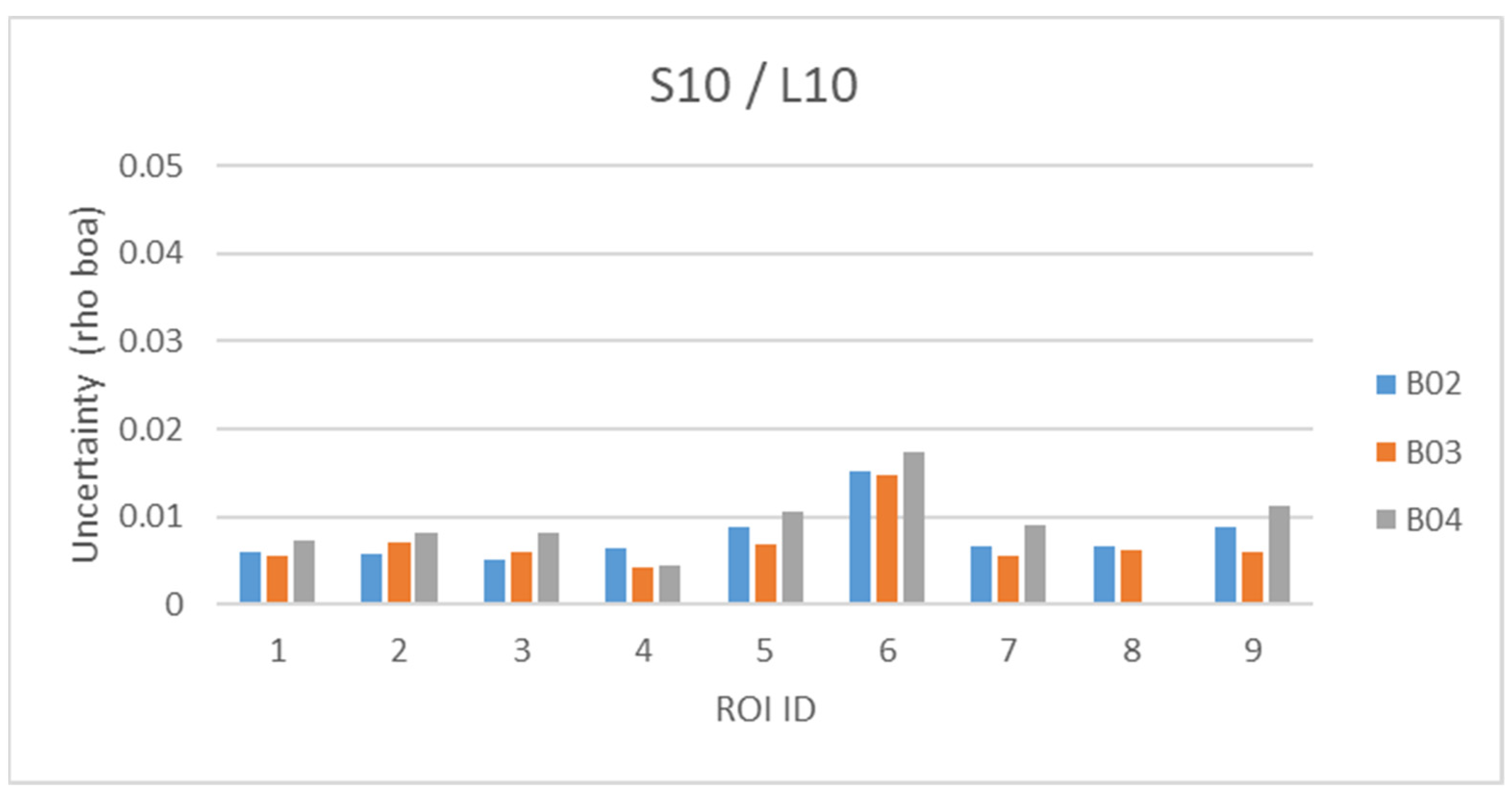
2.5. Data Fusion
- is the final LS8 image at the S2 spatial resolution, with deconvolution from 30 m to 10 m,
- is the original LS8 image resampled from 30 m to 10 m by using bilinear interpolation, which is associated to the phase of signal,
- is the image of differences derived between 30 m and 10 m spatial resolution predicted by using S2 data and associated with the amplitude of the signal.
3. Validation Results
4. Discussions
4.1. The S2L Framework
4.2. Adaptation to Further Optical Missions
5. Conclusions
Author Contributions
Funding
Data Availability Statement
Acknowledgments
Conflicts of Interest
Appendix A. S2L Data Description
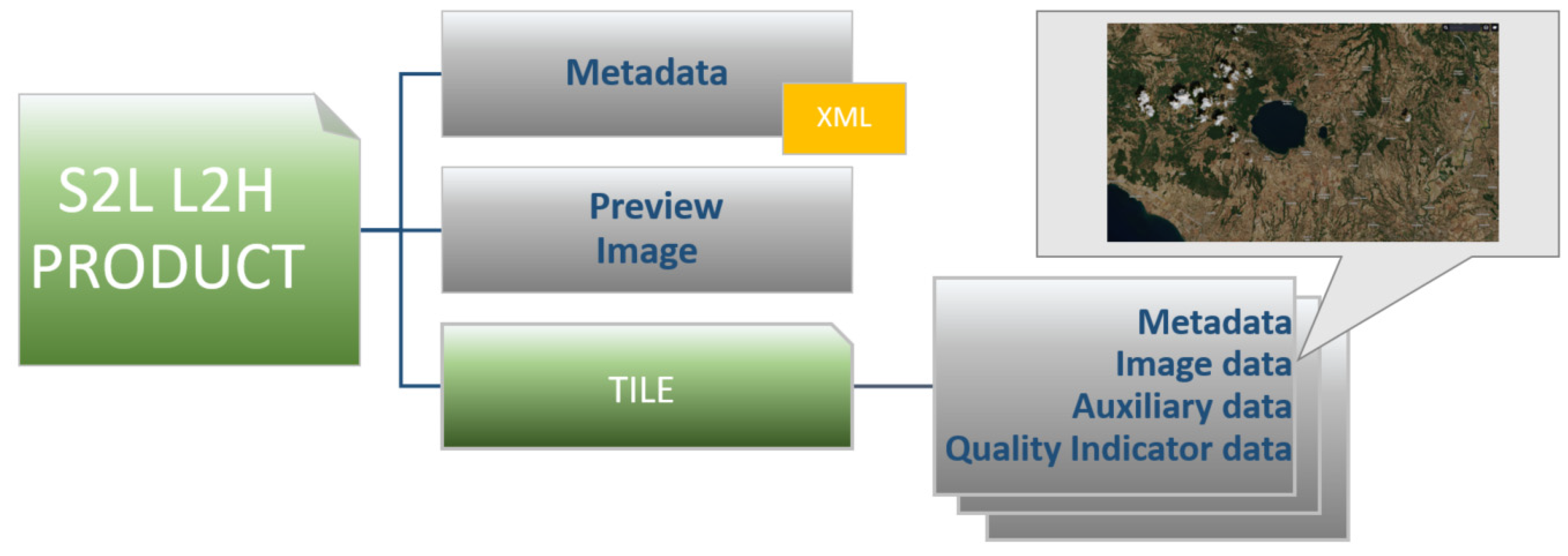
Appendix A.1. Image Data

| Level 2H | Level 2F | |
|---|---|---|
| S2 | The harmonized surface reflectance tiles at Sentinel-2 spatial resolution with 7 bands: B01 (60 m), B02 (10 m), B03 (10 m), B04 (10 m), B8A (20 m), B11 (20 m), B12 (20 m) | |
| LS8 | The harmonized surface reflectance tiles with 7 bands at Landsat-8 spatial resolution (B01, B02, B03, B04, B8A (L05), B11 (L06), B12 (L07) | The fused surface reflectance tiles with 6 bands at Sentinel-2 resolution B02, B03, B04, B8A (L05), B11 (L06), B12 (L07) and with 1 band at Landsat-8 resolution B01 (30 m) |
| NATIVES2 | The surface reflectance tiles at Sentinel-2 spatial resolution with 4 channels B05 (20 m), B06 (20 m), B07 (20 m), B08 (10 m) | |
| NATIVELS8 | The panchromatic surface reflectance tile (15 m) and the 2 emissive bands at 30 m resolution (L10 & L11) | |
| Image Name | Image Format | Resolution | Description |
|---|---|---|---|
| Preview Image | GeoTIFF (8 bit) | 320 m | RGB (3 channels: RED = B4; GREEN = B3; BLUE = B2). Preview dynamic is stretched (min = 0.0, max = 0.250, scale = 255.0) |
| Quicklook Image | JPEG | 30 m | RGB (3 channels: RED = B4; GREEN = B3; BLUE = B2). Preview dynamic is stretched (min = 0.0, max = 0.250, scale = 255.0) |
| Quicklook Image | JPEG | 30m | SWIR-NIR (3 channels: RED = B12; GREEN = B11; BLUE = B8A). Preview dynamic is stretched (min = 0.0, max = 0.40, scale = 255.0) |
Appendix A.2. Metadata
| Metadata Name | Description |
|---|---|
| Product Level | |
| Information |
|
| |
| Processing Level | |
| List of image files L2H/F composing the products | |
| Spectral information (relation between production image channels and on-board spectral bands) Solar irradiance (per band) and the correction U related to the Earth-Sun distance variation | |
| Reflectance quantification value (for conversion of digital numbers into reflectance); | |
| Special values encoding (e.g., NODATA). | |
| Quality Indicator | Cloud coverage assessment |
| Tile Level | |
| Metadata | Tile identifier, as referenced by Level-1C data |
Tile geocoding:
| |
| Mean sun angles (zenith and azimuth) | |
| Mean viewing incidence angles per band (zenith and azimuth) | |
| Quality indicator | Cloudy pixel percentage |
| Pixel level quality indicator: pointer to the QI files Quicklooks and Preview data information: pointer to image files | |
Appendix A.3. Quality Indicator Data
| Name | Description | QI Parameters |
|---|---|---|
| L2A_SceneClass | L2A scene classification QI (Sen2Cor version 2.10 ATBD, available at https://step.esa.int/thirdparties/sen2cor/2.10.0/docs/S2-PDGS-MPC-L2A-ATBD-V2.10.0.pdf accessed on 7 July 2022) | Percentage of classified pixels |
| L2A_AtmCorr | L2A atmospheric correction QI (Sen2Cor version 2.10 ATBD, available at https://step.esa.int/thirdparties/sen2cor/2.10.0/docs/S2-PDGS-MPC-L2A-ATBD-V2.10.0.pdf accessed on 7 July 2022) | Average values of atmospheric parameters (ozone, water vapor, aerosol) Average solar zenith angle |
| Auxiliary Data | Digital Elevation Model QI, Meteorological data QI | Place reserved, intended for Sen2like 4.2 |
| L2{H,F}_Geometry | Reference of the method (string) QI derived from the geometric assessment processing | BAND, COREGISTRATION BEFORE_CORRECTION, COREGISTRATION AFTER_CORRECTION, NB_OF_POINTS, MEAN, STD, RMSE, SKEW, KURTOSIS [22,23,24,25] |
| L2{H,F}_BRDF_NBAR | Reference of the method (string) QI derived from the BRDF processing | KERNEL_DEFINITION, CONSTANT SOLAR_ZENITH_ANGLE, MEAN DELTA_AZIMUTH [38,39] |
| L2{H,F}_SBAF | Reference of the method (string) SBAF coefficients and offsets (values) | SBAF coefficients and offsets per band [8] |
| L2F_FUS L2F only | Reference of the method (string) QI derived from the processing | Sen2like ATBD (unpublished) |
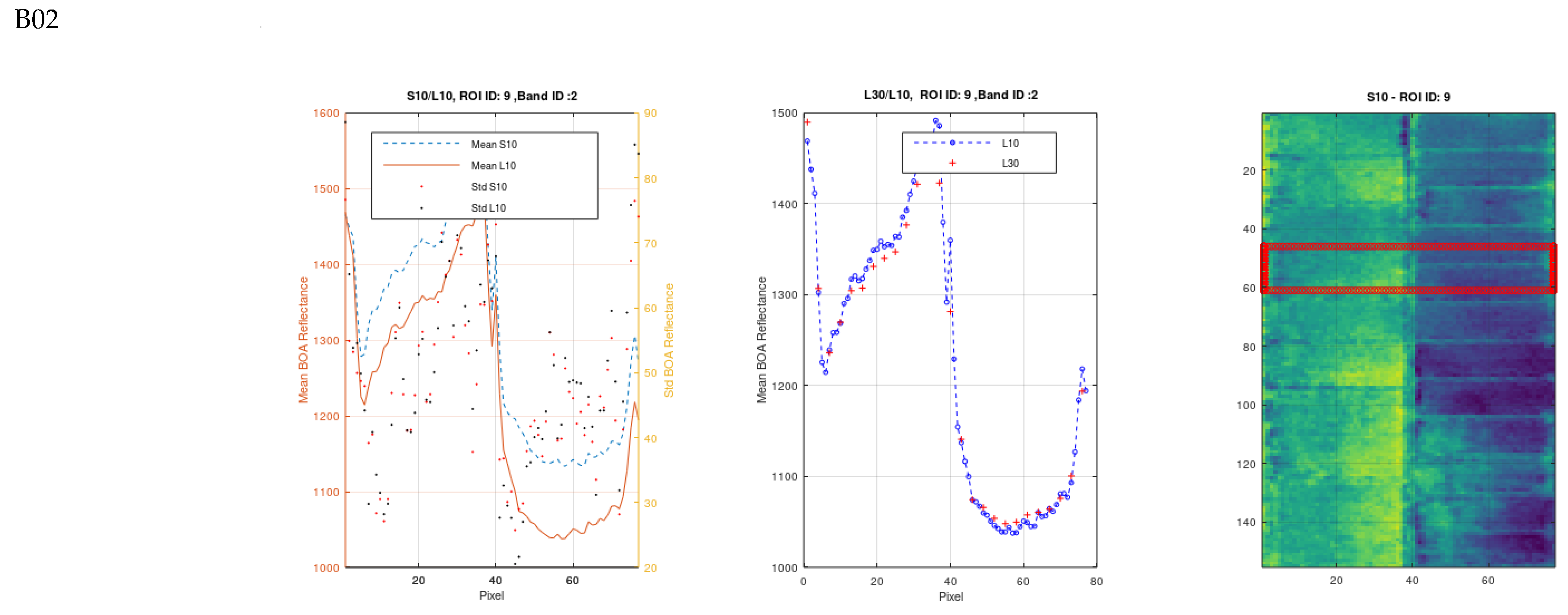
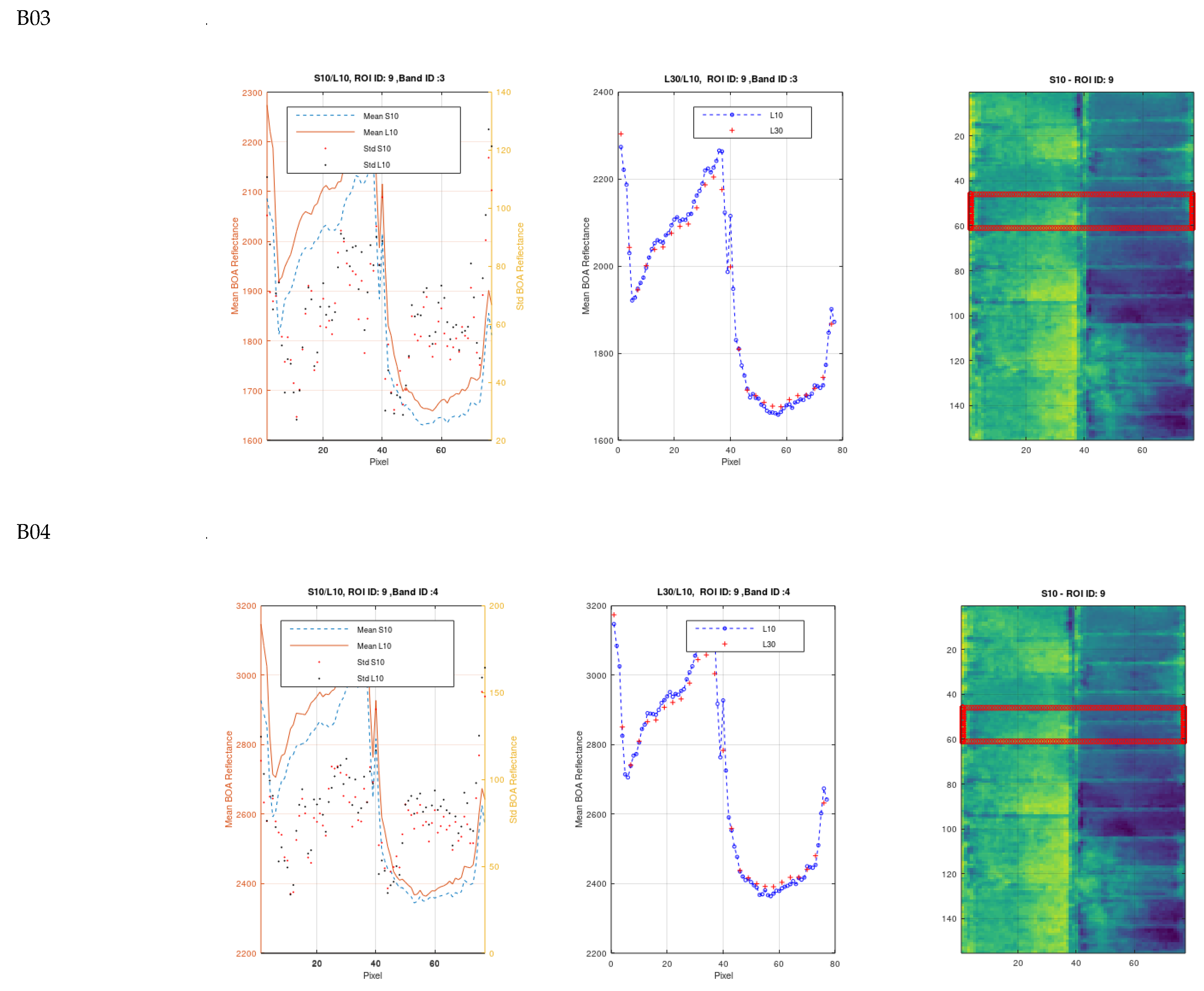
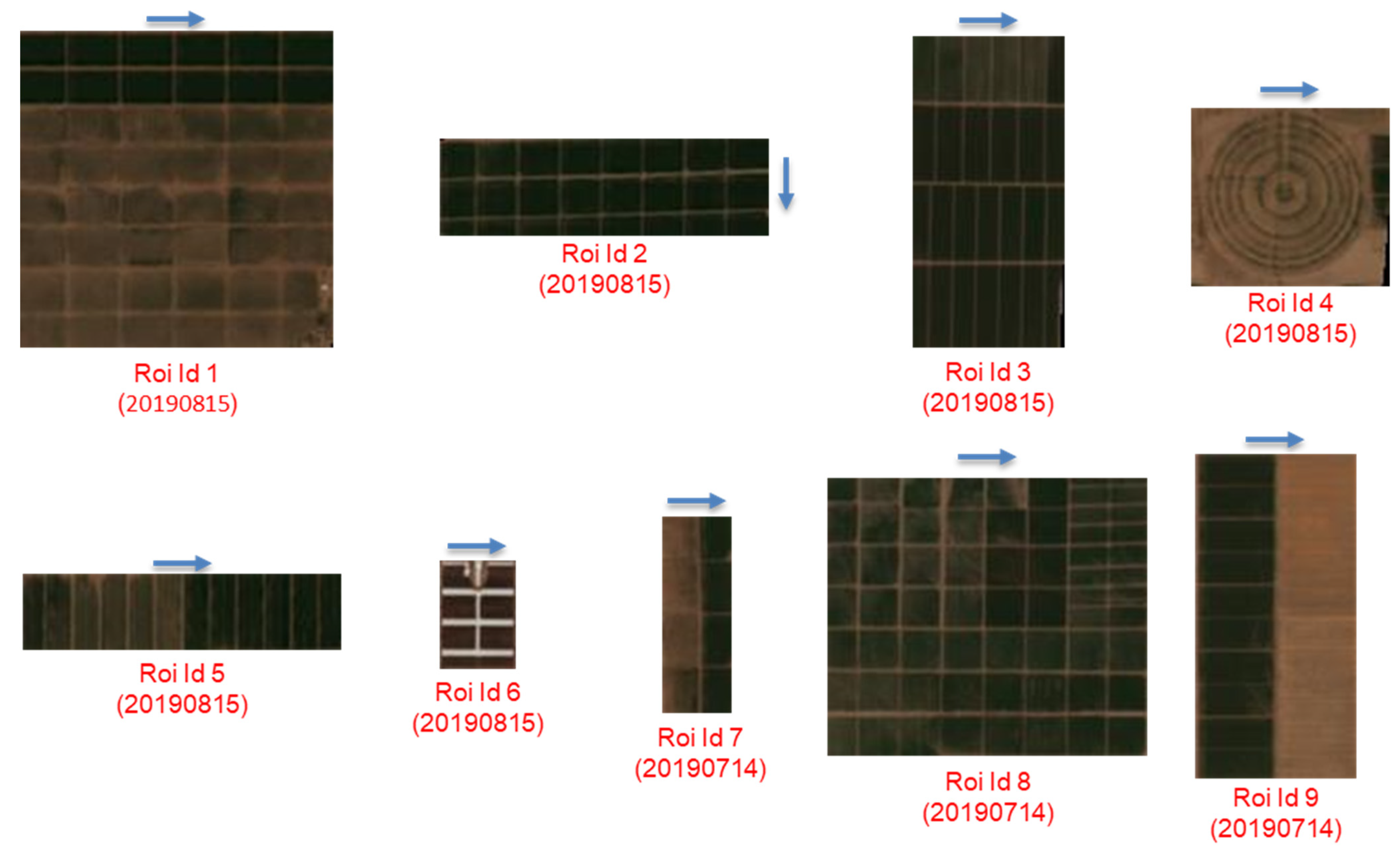
Appendix B. Validation of Data Fusion Algorithm


References
- Drusch, M.; Del Bello, U.; Carlier, S.; Colin, O.; Fernandez, V.; Gascon, F.; Hoersch, B.; Isola, C.; Laberinti, P.; Martimort, P.; et al. Sentinel-2: ESA’s optical high-resolution mission for GMES operational services. Remote Sens. Environ. 2012, 120, 25–36. [Google Scholar] [CrossRef]
- ESA Sentinel-2: ESA’s Optical High-Resolution Mission for GMES Operational Services, ESA SP-1322/2 March 2012, ESA Communications, ESTEC. Available online: https://sentinel.esa.int/documents/247904/349490/s2_sp-1322_2.pdf (accessed on 7 July 2022).
- Li, J.; Chen, B. Global Revisit Interval Analysis of Landsat-8 -9 and Sentinel-2A -2B Data for Terrestrial Monitoring. Sensors 2020, 20, 6631. [Google Scholar] [CrossRef] [PubMed]
- Belward, A.S.; Skøien, J.O. Who launched what, when and why; trends in global land-cover observation capacity from civilian earth observation satellites. ISPRS J. Photogramm. Remote Sens. 2015, 103, 115–128. [Google Scholar] [CrossRef]
- ARD Zone. Available online: https://www.ard.zone/ard20 (accessed on 5 July 2022).
- CEOS Analysis Ready Data for Land. Product Family Specification, Surface Reflectance (CARD4L-SR). Available online: https://ceos.org/ard/files/PFS/SR/v5.0/CARD4L_Product_Family_Specification_Surface_Reflectance-v5.0.pdf (accessed on 5 July 2022).
- Giuliani, G.; Camara, G.; Killough, B.; Minchin, S. Earth Observation Open Science: Enhancing Reproducible Science Using Data Cubes. Data 2019, 4, 147. [Google Scholar] [CrossRef] [Green Version]
- Claverie, M.; Ju, J.; Masek, J.G.; Dungan, J.L.; Vermote, E.F.; Roger, J.C.; Skakun, S.V.; Justice, C. The Harmonized Landsat and Sentinel-2 surface reflectance data set. Remote Sens. Environ. 2018, 219, 145–161. [Google Scholar] [CrossRef]
- Frantz, D. FORCE—Landsat+ Sentinel-2 analysis ready data and beyond. Remote Sens. 2019, 11, 1124. [Google Scholar] [CrossRef] [Green Version]
- Hagolle, O.; Huc, M.; Descardins, C.; Auer, S.; Richter, R. MAJA Algorithm Theoretical Basis Document. Available online: https://doi.org/10.5281/zenodo.1209633 (accessed on 5 July 2022).
- Planet Fusion Monitoring Technical Specification Version 1.0.0-beta.3, March 2021, Calibration, Analysis Ready Data, and Inter Operability (CARDIO) Operations. Available online: https://assets.planet.com/docs/Planet_fusion_specification_March_2021.pdf (accessed on 5 July 2022).
- Saunier, S.; Louis, J.; Debaecker, V.; Beaton, T.; Cadau, E.G.; Boccia, V.; Gascon, F. Sen2like, a tool to generate Sentinel-2 harmonised surface reflectance products-first results with Landsat-8. In Proceedings of the IGARSS 2019-2019 IEEE International Geoscience and Remote Sensing Symposium, Yokohama, Japan, 28 July–2 August 2019; IEEE: Piscataway, NJ, USA, 2019; pp. 5650–5653. [Google Scholar] [CrossRef]
- S2 MSI ESL team, Data Quality Report Sentinel-2 MSI L1C/L2A. Available online: https://sentinels.copernicus.eu/web/sentinel/data-product-quality-reports (accessed on 5 July 2022).
- Wulder, M.A.; Hilker, T.; White, J.C.; Coops, N.C.; Masek, J.G.; Pflugmacher, D.; Crevier, Y. Virtual constellations for global terrestrial monitoring. Remote Sens. Environ. 2015, 170, 62–76. [Google Scholar] [CrossRef] [Green Version]
- ESA Sentinel-2 User Handbook. Available online: https://sentinels.copernicus.eu/web/sentinel/user-guides/document-library/-/asset_publisher/xlslt4309D5h/content/sentinel-2-user-handbook (accessed on 5 July 2022).
- Copernicus Access Hub. Available online: https://scihub.copernicus.eu (accessed on 5 July 2022).
- ESA Landsat 8 Data Portal. Available online: https://landsat8portal.eo.esa.int (accessed on 5 July 2022).
- Sentinel-2 Products Specification Document, S2-PDGS-TAS-DI-PSD.; Issue 14.9, 30/09/2021. Available online: https://sentinels.copernicus.eu/documents/247904/685211/S2-PDGS-TAS-DI-PSD-V14.9.pdf/3d3b6c9c-4334-dcc4-3aa7-f7c0deffbaf7?t=1643013091529 (accessed on 5 July 2022).
- Cloud Optimized GeoTIFF (COG). Available online: https://www.cogeo.org (accessed on 5 July 2022).
- Spatio Temporal Asset Catalog Specification. Available online: https://stacspec.org/en (accessed on 5 July 2022).
- CAMS Service. Available online: https://atmosphere.copernicus.eu/ (accessed on 5 July 2022).
- Tomasi, C.; Kanade, T. Detection and tracking of point. Int. J. Comput. Vis. 1991, 9, 137–154. [Google Scholar] [CrossRef]
- Lucas, B.D.; Kanade, T. An iterative image registration technique with an application to stereo vision. In Proceedings of the 7th International Joint Conference on Artificial Intelligence, Vancouver, BC, Canada, 24–28 August 1981; pp. 674–679. [Google Scholar]
- OpenCV Optical Flow. Available online: https://docs.opencv.org/3.4/d4/dee/tutorial_optical_flow.html (accessed on 5 July 2022).
- Bouguet, J.Y. Pyramidal implementation of the affine Lucas Kanade feature tracker description of the algorithm. Intel Corp. 2001, 5, 4. [Google Scholar]
- Shi, J.; Tomasi, C. Good features to track. In Proceedings of the IEEE Computer Society Conference on Computer Vision and Pattern Recognition 1994, Seattle, WA, USA, 21–23 June 1997; pp. 593–600. [Google Scholar]
- Debaecker, V.; Kocaman, S.; Saunier, S.; Garcia, K.; Bas, S.; Just, D. On the geometric accuracy and stability of MSG SEVIRI images. Atmos. Environ. 2021, 262, 118645. [Google Scholar] [CrossRef]
- Bas, S.; Debaecker, V.; Kocaman, S.; Saunier, S.; Garcia, K.; Just, D. Investigations on the Geometric Quality of AVHRR Level 1B Imagery Aboard MetOp-A. PFG–J. Photogramm. Remote Sens. Geoinf. Sci. 2021, 89, 519–534. [Google Scholar] [CrossRef]
- Kocaman, S.; Debaecker, V.; Bas, S.; Saunier, S.; Garcia, K.; Just, D. A comprehensive geometric quality assessment approach for MSG SEVIRI imagery. Adv. Space Res. 2022, 69, 1462–1480. [Google Scholar] [CrossRef]
- Aksakal, S.K.; Neuhaus, C.; Baltsavias, E.; Schindler, K. Geometric quality analysis of AVHRR orthoimages. Remote Sens. 2015, 7, 3293–3319. [Google Scholar] [CrossRef] [Green Version]
- Aksakal, S.K. Geometric accuracy investigations of SEVIRI high resolution visible (HRV) level 1.5 Imagery. Remote Sens. 2013, 5, 2475–2491. [Google Scholar] [CrossRef] [Green Version]
- Kocaman, S.; Debaecker, V.; Bas, S.; Saunier, S.; Garcia, K.; Just, D. Investigations on the Global Image Datasets for the Absolute Geometric Quality Assessment of MSG SEVIRI Imagery. Int. Arch. Photogramm. Remote Sens. Spat. Inf. Sci. 2020, 43, 1339–1346. [Google Scholar] [CrossRef]
- Rahman, H.; Dedieu, G. SMAC: A simplified method for the atmospheric correction of satellite measurements in the solar spectrum. Int. J. Remote Sens. 1994, 15, 123–143. [Google Scholar] [CrossRef]
- CESBIO repository for SMAC coefficients. Available online: http://www.cesbio.ups-tlse.fr/fr/smac_telech.htm (accessed on 5 July 2022).
- Zhu, Z.; Woodcock, C.E. Object-based cloud and cloud shadow detection in Landsat imagery. Remote Sens. Environ. 2012, 118, 83–94. [Google Scholar] [CrossRef]
- Main-Knorn, M.; Pflug, B.; Louis, J.; Debaecker, V.; Müller-Wilm, U.; Gascon, F. Sen2Cor for sentinel-2. In Image and Signal Processing for Remote Sensing XXIII; SPIE: Bellingham, WA, USA, 2017; Volume 10427, pp. 37–48. [Google Scholar] [CrossRef] [Green Version]
- Doxani, G.; Vermote, E.; Roger, J.-C.; Gascon, F.; Adriaensen, S.; Frantz, D.; Hagolle, O.; Hollstein, A.; Kirches, G.; Li, F.; et al. Atmospheric Correction Inter-Comparison Exercise. Remote Sens. 2018, 10, 352. [Google Scholar] [CrossRef] [Green Version]
- Vermote, E.; Justice, C.O.; Bréon, F.M. Towards a generalized approach for correction of the BRDF effect in MODIS directional reflectances. IEEE Trans. Geosci. Remote Sens. 2008, 47, 898–908. [Google Scholar] [CrossRef]
- Roy, D.P.; Zhang, H.K.; Ju, J.; Gomez-Dans, J.L.; Lewis, P.E.; Schaaf, C.B.; Sun, Q.; Li, J.; Huang, H.; Kovalskyy, V. A general method to normalize Landsat reflectance data to nadir BRDF adjusted reflectance. Remote Sens. Environ. 2016, 176, 255–271. [Google Scholar] [CrossRef] [Green Version]
- Roy, D.P.; Li, J.; Zhang, H.K.; Yan, L.; Huang, H.; Li, Z. Examination of Sentinel-2A multi-spectral instrument (MSI) reflectance anisotropy and the suitability of a general method to normalize MSI reflectance to nadir BRDF adjusted reflectance. Remote Sens. Environ. 2017, 199, 25–38. [Google Scholar] [CrossRef]
- Franch, B.; Vermote, E.F.; Claverie, M. Intercomparison of Landsat albedo retrieval techniques and evaluation against in situ measurements across the USA surfrad network. Remote Sens. Environ. 2014, 152, 627–637. [Google Scholar] [CrossRef]
- Gao, F.; Masek, J.; Schwaller, M.; Hall, F. On the blending of the Landsat and MODIS surface reflectance: Predicting daily Landsat surface reflectance. IEEE Trans. Geosci. Remote Sens. 2006, 44, 2207–2218. [Google Scholar]
- Claverie, M.; Vermote, E.; Franch, B.; He, T.; Hagolle, O.; Kadiri, M.; Masek, J. Evaluation of Medium Spatial Resolution BRDF-Adjustment Techniques Using Multi-Angular SPOT4 (Take5) Acquisitions. Remote Sens. 2015, 7, 12057–12075. [Google Scholar] [CrossRef] [Green Version]
- Johnson, D.M.; Mueller, R. The 2009 cropland data layer. Photogramm. Eng. Remote Sens. 2010, 76, 1201–1205. [Google Scholar]
- Maignan, F.; Bréon, F.-M.; Lacaze, R. Bidirectional reflectance of Earth targets: Evaluation of analytical models using a large set of spaceborne measurements with emphasis on the Hot Spot. Remote Sens. Environ. 2004, 90, 210–220. [Google Scholar] [CrossRef]
- Li, X.; Strahler, A.H. Geometric-optical bidirectional reflectance modeling of a conifer forest canopy. IEEE Transactions on Geosci. Remote Sens. 1986, GE-24, 906–919. [Google Scholar] [CrossRef]
- Schaaf, C.B.; Gao, F.; Strahler, A.H.; Lucht, W.; Li, X.; Tsang, T.; Strugnell, N.C.; Zhang, X.; Jin, Y.; Muller, J.-P.; et al. First operational BRDF, albedo nadir reflectance products from MODIS. Remote Sens. Environ. 2002, 83, 135–148. [Google Scholar] [CrossRef] [Green Version]
- Skakun, S.; Ju, J.; Claverie, M.; Roger, J.C.; Vermote, E.; Franch, B.; Dungan, J.L.; Masek, J. Harmonized Landsat Sentinel-2 (HLS) Product User’s Guide. Version 1.4, October 2018. Available online: https://hls.gsfc.nasa.gov/wp-content/uploads/2019/01/HLS.v1.4.UserGuide_draft_ver3.1.pdf (accessed on 5 July 2022).
- Franch, B.; Vermote, E.; Skakun, S.; Roger, J.C.; Masek, J.; Ju, J.; Villaescusa-Nadal, J.L.; Santamaria-Artigas, A. A method for Landsat and Sentinel 2 (HLS) BRDF normalization. Remote Sens. 2019, 11, 632. [Google Scholar] [CrossRef] [Green Version]
- Villaescusa-Nadal, J.L.; Franch, B.; Vermote, E.F.; Roger, J.C. Improving the AVHRR long term data record BRDF correction. Remote Sens. 2019, 11, 502. [Google Scholar] [CrossRef] [Green Version]
- Baret, F.; Morissette, J.T.; Fernandes, R.A.; Champeaux, J.L.; Myneni, R.B.; Chen, J.; Plummer, S.; Weiss, M.; Bacour, C.; Garrigues, S.; et al. Evaluation of the representativeness of networks of sites for the global validation and intercomparison of land biophysical products: Proposition of the CEOS-BELMANIP. IEEE Trans. Geosci. Remote Sens. 2006, 44, 1794–1803. [Google Scholar] [CrossRef]
- Teillet, P.M.; Fedosejevs, G.; Thome, K.J.; Barker, J.L. Impacts of spectral band difference effects on radiometric cross-calibration between satellite sensors in the solar-reflective spectral domain. Remote Sens. Environ. 2007, 110, 393–409. [Google Scholar] [CrossRef]
- Barsi, J.A.; Alhammoud, B.; Czapla-Myers, J.; Gascon, F.; Haque, O.; Kaewmanee, M.; Leigh, L.; Markham, B.L. Sentinel-2A MSI and Landsat-8 OLI radiometric cross comparison over desert sites. Eur. J. Remote Sens. 2018, 51, 822–837. [Google Scholar] [CrossRef]
- Landsat Collection 1 Level-1 Quality Assessment Band. Available online: https://www.usgs.gov/landsat-missions/landsat-collection-1-level-1-quality-assessment-band (accessed on 17 June 2022).
- Landsat Collection 2 Quality Assessment Bands. Available online: https://www.usgs.gov/landsat-missions/landsat-collection-2-quality-assessment-bands (accessed on 17 June 2022).
- Louis, J. Sentinel-2 Level-2A Algorithm Theoretical Basis Document. 2021. Available online: https://sentinels.copernicus.eu/documents/247904/446933/Sentinel-2-Level-2A-Algorithm-Theoretical-Basis-Document-ATBD.pdf (accessed on 17 June 2022).
- Skakun, S.; Wevers, J.; Brockmann, C.; Doxani, G.; Aleksandrov, M.; Batič, M.; Frantz, D.; Gascon, F.; Gómez-Chova, L.; Hagolle, O.; et al. Cloud Mask Intercomparison eXercise (CMIX): An evaluation of cloud masking algorithms for Landsat 8 and Sentinel-2. Remote Sens. Environ. 2022, 274, 112990. [Google Scholar] [CrossRef]
- Filgueiras, R.; Mantovani, E.C.; Fernandes-Filho, E.I.; Cunha, F.F.D.; Althoff, D.; Dias, S.H.B. Fusion of MODIS and Landsat-Like images for daily high spatial resolution NDVI. Remote Sens. 2020, 12, 1297. [Google Scholar] [CrossRef] [Green Version]
- Gevaert, C.M.; García-Haro, F.J. A comparison of STARFM and an unmixing-based algorithm for Landsat and MODIS data fusion. Remote Sens. Environ. 2015, 156, 34–44. [Google Scholar] [CrossRef]
- Zhu, X.; Cai, F.; Tian, J.; Williams, T.K.-A. Spatiotemporal Fusion of Multisource Remote Sensing Data: Literature Survey, Taxonomy, Principles, Applications, and Future Directions. Remote Sens. 2018, 10, 527. [Google Scholar] [CrossRef] [Green Version]
- ESA: Land Cover CCI Product User Guide Version 2.0. 2017. Available online: http://maps.elie.ucl.ac.be/CCI/viewer/download/ESACCI-LC-Ph2-PUGv2_2.0.pdf (accessed on 5 July 2022).
- Vermote, E.F.; Kotchenova, S.Y. Atmospheric correction for the monitoring of land surfaces. J. Geophys. Res. 2008, 113, D23S90. [Google Scholar] [CrossRef]
- EO portal directory, Resourcesat-2. Available online: https://directory.eoportal.org/web/eoportal/satellite-missions/r/resourcesat-2 (accessed on 5 July 2022).
- Alonso, K.; Bachmann, M.; Burch, K.; Carmona, E.; Cerra, D.; de los Reyes, R.; Dietrich, D.; Heiden, U.; Hölderlin, A.; Ickes, J.; et al. Data Products, Quality and Validation of the DLR Earth Sensing Imaging Spectrometer (DESIS). Sensors 2019, 19, 4471. [Google Scholar] [CrossRef] [Green Version]
- Barry, P.S.; Mendenhall, J.; Jarecke, P.; Folkman, M.; Pearlman, J.; Markham, B. EO-1 Hyperion hyperspectral aggregation and comparison with EO-1 Advanced Land Imager and Landsat 7 ETM+. In Proceedings of the IEEE International Geoscience and Remote Sensing Symposium, Toronto, ON, Canada, 24–28 June 2002; Volume 3, pp. 1648–1651. [Google Scholar] [CrossRef]
- Guarini, R.; Loizzo, R.; Longo, F.; Mari, S.; Scopa, T.; Varacalli, G. Overview of the prisma space and ground segment and its hyperspectral products. In Proceedings of the 2017 IEEE International Geoscience and Remote Sensing Symposium (IGARSS), Fort Worth, TX, USA, 23–28 July 2017; pp. 431–434. [Google Scholar] [CrossRef]
- Guanter, L.; Kaufmann, H.; Segl, K.; Foerster, S.; Rogass, C.; Chabrillat, S.; Kuester, T.; Hollstein, A.; Rossner, G.; Chlebek, C.; et al. The EnMAP Spaceborne Imaging Spectroscopy Mission for Earth Observation. Remote Sens. 2015, 7, 8830–8857. [Google Scholar] [CrossRef] [Green Version]
- Rast, M.; Nieke, J.; Adams, J.; Isola, C.; Gascon, F. Copernicus Hyperspectral Imaging Mission for the Environment (Chime). In Proceedings of the 2021 IEEE International Geoscience and Remote Sensing Symposium IGARSS, Brussels, Belgium, 11–16 July 2021; IEEE: Piscataway, NJ, USA, 2021; pp. 108–111. [Google Scholar] [CrossRef]
- Gross, G.; Helder, D.; Begeman, C.; Leigh, L.; Kaewmanee, M.; Shah, R. Initial Cross-Calibration of Landsat 8 and Landsat 9 Using the Simultaneous Underfly Event. Remote Sens. 2022, 14, 2418. [Google Scholar] [CrossRef]
- Cornebise, J.; Oršolić, I.; Kalaitzis, F. Open High-Resolution Satellite Imagery: The WorldStrat Dataset—With Application to Super-Resolution. arXiv 2022, arXiv:2207.06418. [Google Scholar]


| S2L Band | Band Designation | S2 MSI Bands (Center Wavelength [µm]) | LS8/LS9 OLI/TIRS Bands (Center Wavelength [µm]) | L2H S2 Resolution(m) | L2H- LS8/LS9 Resolution (m) | L2F S2 Resolution (m) | L2F LS8/LS9 Resolution (m) |
|---|---|---|---|---|---|---|---|
| B01 | Coastal Aerosol | B01 (443 nm) | B01 (442 nm) | 60 | 30 | 60 | 30 |
| B02 | Blue | B02 (490 nm) | B02 (482 nm) | 10 | 30 | 10 | 10 |
| B03 | Green | B03 (560nm) | B03 (561 nm) | 10 | 30 | 10 | 10 |
| B04 | Red | B04 (665 nm) | B04 (654 nm) | 10 | 30 | 10 | 10 |
| B08 | NIR 1 | B08 (842 nm) | None 1 | 10 | - | 10 | - |
| B8A | NIR2 | B8A (865 nm) | B05 (864 nm) | 20 | 30 | 20 | 20 |
| B11 | SWIR 1 | B11 (1610 nm) | B06 (1608 nm) | 20 | 30 | 20 | 20 |
| B12 | SWIR 2 | B12 (2190 nm) | B07 (2200 nm) | 20 | 30 | 20 | 20 |
| BP1 | Panchromatic | None 2 | B08 (589 nm) | - | 15 | - | 15 |
| BT1 | TIRS 1 | None 2 | B10 (11 µm) | - | 100 | - | 100 |
| BT2 | TIRS 2 | None 2 | B11 (12.2 µm) | - | 100 | - | 100 |
| B05 | Red Edge 1 | B05 (705 nm) | None 1 | 20 | - | 20 | |
| B06 | Red Edge 2 | B06 (740 nm) | None 1 | 20 | - | 20 | |
| B07 | Red Edge 3 | B07 (783 nm) | None 1 | 20 | - | 20 |
| Algorithm | BRDF Approach | BRDF Dynamic | Use of HR NDVI | Use of MR BRDF | Land Cover | BRDF Coefficients at HR |
|---|---|---|---|---|---|---|
| C-factor 1 [39,40] | MCD43 | No BRDF dynamic | No | No | No | No |
| LUM [42] | MCD43 | spatial and temporal variations | No | MCD43 at 500 m | Yes (CDL2) | Yes (but per crop) |
| VI-dis [43] | VJB | Spatial and temporal variation | Yes | MODIS VJB at 1250 m | No | No |
| HABA [41] | VJB | Spatial and temporal variation | Yes | MODIS VJB at 1000 m | Yes | Yes |
| 31.0076 | −0.1272 | 0.01187 | 2.40 × 10⁻⁵ | −9.48 × 10⁻⁹ | −1.95 × 10⁻⁹ | 6.15 × 10⁻¹¹ |
| Band | Method | Mean | Std | % Corr |
|---|---|---|---|---|
| B02 | DIR | 0.01297 | 0.01174 | |
| C-FACTOR | 0.01482 | 0.01402 | 14.24% | |
| HABA | 0.01213 | 0.01139 | −6.45% | |
| B03 | DIR | 0.01179 | 0.01207 | |
| C-FACTOR | 0.01397 | 0.01460 | 18.56% | |
| HABA | 0.01062 | 0.01185 | −9.90% | |
| B04 | DIR | 0.01144 | 0.01318 | |
| C-FACTOR | 0.01357 | 0.01552 | 18.58% | |
| HABA | 0.01051 | 0.01279 | −8.19% | |
| B8A | DIR | 0.01994 | 0.02038 | |
| C-FACTOR | 0.02431 | 0.02213 | 21.96% | |
| HABA | 0.01742 | 0.02002 | −12.60% | |
| B11 | DIR | 0.01424 | 0.01842 | |
| C-FACTOR | 0.01753 | 0.02012 | 23.03% | |
| HABA | 0.01243 | 0.01791 | −12.74% | |
| B12 | DIR | 0.02621 | 0.01686 | |
| C-FACTOR | 0.03134 | 0.01851 | 19.58% | |
| HABA | 0.02442 | 0.01614 | −6.82% |
| Pixel Number | Mean S2A | Mean LS8 | LS8/S2A | Accuracy (A) | Precision (P) | Uncertainty (U) | ||
|---|---|---|---|---|---|---|---|---|
| L2H (30 m) | B02 | 99,346 | 0.109 | 0.103 | 0.945 | 0.006 | 0.008 | 0.010 |
| B03 | 99,358 | 0.149 | 0.148 | 0.996 | 0.001 | 0.009 | 0.009 | |
| B04 | 99,321 | 0.205 | 0.201 | 0.980 | 0.004 | 0.012 | 0.013 | |
| L2F (10 m) | B02 | 99,159 | 0.109 | 0.103 | 0.944 | 0.006 | 0.007 | 0.009 |
| B03 | 99,208 | 0.149 | 0.148 | 0.996 | 0.001 | 0.008 | 0.008 | |
| B04 | 99,380 | 0.205 | 0.201 | 0.980 | 0.004 | 0.010 | 0.011 | |
Publisher’s Note: MDPI stays neutral with regard to jurisdictional claims in published maps and institutional affiliations. |
© 2022 by the authors. Licensee MDPI, Basel, Switzerland. This article is an open access article distributed under the terms and conditions of the Creative Commons Attribution (CC BY) license (https://creativecommons.org/licenses/by/4.0/).
Share and Cite
Saunier, S.; Pflug, B.; Lobos, I.M.; Franch, B.; Louis, J.; De Los Reyes, R.; Debaecker, V.; Cadau, E.G.; Boccia, V.; Gascon, F.; et al. Sen2Like: Paving the Way towards Harmonization and Fusion of Optical Data. Remote Sens. 2022, 14, 3855. https://doi.org/10.3390/rs14163855
Saunier S, Pflug B, Lobos IM, Franch B, Louis J, De Los Reyes R, Debaecker V, Cadau EG, Boccia V, Gascon F, et al. Sen2Like: Paving the Way towards Harmonization and Fusion of Optical Data. Remote Sensing. 2022; 14(16):3855. https://doi.org/10.3390/rs14163855
Chicago/Turabian StyleSaunier, Sébastien, Bringfried Pflug, Italo Moletto Lobos, Belen Franch, Jérôme Louis, Raquel De Los Reyes, Vincent Debaecker, Enrico G. Cadau, Valentina Boccia, Ferran Gascon, and et al. 2022. "Sen2Like: Paving the Way towards Harmonization and Fusion of Optical Data" Remote Sensing 14, no. 16: 3855. https://doi.org/10.3390/rs14163855
APA StyleSaunier, S., Pflug, B., Lobos, I. M., Franch, B., Louis, J., De Los Reyes, R., Debaecker, V., Cadau, E. G., Boccia, V., Gascon, F., & Kocaman, S. (2022). Sen2Like: Paving the Way towards Harmonization and Fusion of Optical Data. Remote Sensing, 14(16), 3855. https://doi.org/10.3390/rs14163855