Wide-Area GNSS Corrections for Precise Positioning and Navigation in Agriculture

Abstract

This paper characterizes, with static and roving GNSS receivers in the context of precision agriculture research, the hybrid ionospheric-geodetic GNSS model Wide-Area Real-Time Kinematics (WARTK), which computes and broadcasts real-time corrections for high-precision GNSS positioning and navigation within sparse GNSS receiver networks. This research is motivated by the potential benefits of the low-cost precise WARTK technique on mass-market applications such as precision agriculture. The results from two experiments summarized in this work, the second one involving a working spraying tractor, show, firstly, that the corrections from the model are in good agreement with the corrections provided by IGS (International GNSS Services) analysis centers computed in post-processing from global GNSS data. Moreover, secondly and most importantly, we have shown that WARTK provides navigation solutions at decimeter-level accuracy, and the ionospheric corrections significantly reduce the computational time for ambiguity estimation: up to convergence times for the 50%, 75% and 95% of cases equal or below 30 s (single-epoch), 150 s and 600 s approximately, vs. 1000 s, 2750 s and 4850 s without ionospheric corrections, everything for a roving receiver at more than 100 km far away from the nearest permanent receiver. The real-time horizontal position errors reach up to 3 cm, 5 cm and 12 cm for 50%, 75% and 95% of cases, respectively, by constraining and continuously updating the ambiguities without updating the permanent receiver coordinates, vs. the 6 cm, 12 cm and 32 cm, respectively, in the same conditions but without WARTK ionospheric corrections.

1. Introduction

The capability of any GNSS model to achieve high accuracy in positioning and navigation depends on the measurement and/or estimation of all sources of perturbations on the code and/or carrier-phase across all frequencies. This is especially true when wide-area permanent networks (with inter-receiver distances of hundreds of km) are the only ones available. As it has been demonstrated in previous works, such high and fast positioning and navigation accuracy of roving GNSS users is only feasible when precise ionospheric corrections are available in real time, like in the case of the Wide-Area Real-Time Kinematics (WARTK [1]). Moreover, differential correction techniques applied to Global Navigation Satellite Systems (GNSS) remove positioning error sources, such as, for example, satellite clocks and delay code/phase bias (DCB, DPB), which are common to the moving receiver (rover) and the base station. Such techniques are limited to areas where either the positioning errors are the same for both the rover and base station, or they are highly correlated in space. In case the observables from the rover and base station are not the same but nonetheless correlated, Network Real-Time Kinematics (NRTK) techniques provide information to the user, based on the modeling of such spatial correlations, but limited to shorter distances (up to some tens of kilometers) than the wide-area network ones (up to hundreds of kilometers).

Alternatively to GNSS positioning using differential correction technique, other methods provide external corrections in the state space for, e.g., satellite orbits, phase delay and/or code biases, and atmospheric corrections. For example, the PPP (Precise Point Positioning [2]) technique uses corrections for the satellite orbit and clocks which are provided by a Central Processing Facility (CPF), thus achieving high positioning accuracy. However, it takes at least half an hour to fix the ambiguity term for PPP algorithms. In order to reduce the computational time for ambiguity fixing, external corrections for the ionospheric term are required [3,4]. There are several methods that use the ionospheric information for GNSS algorithms to converge faster, e.g., undifferenced and uncombined methods, such as PPP-RTK [5,6,7], but also undifferenced and combined methods such as WARTK [1]. Whereas PPP only uses the Ionosphere-Free combination of GNSS measurements, WARTK adds the Geometry-Free combination of the GNSS measurements in order to use the information from the ionosphere to boost the baseline length (from tens to hundreds of km). Moreover, the computational burden of the ambiguity estimation process is relatively low, without the need of fixing it. Furthermore, WARTK exploits the redundancy between the ambiguities from the Geometry-Free, Ionospheric-Free and Melbourne-Wübbena combinations, thereby estimating the ambiguities for each frequency. Network RTK and RTK methods also provide high accuracy and precision for navigation and positioning in real time, although they both require denser networks than PPP-RTK and WARTK.

This paper shows how WARTK can provide the necessary corrections for high-accuracy positioning and navigation algorithms for rovers, also in the context of precision agriculture research, thus bringing the standard PPP model into RTK applications. The next section introduces and develops the WARTK equations. Then, the third section summarizes the external assessment of WARTK corrections generated from the network GNSS measurements. The fourth section summarizes the performance at WARTK roving user level in two experiments, including a real-case precision agriculture scenario in the Netherlands. The final section provides the conclusions.

2. The WARTK Model

WARTK was first introduced to provide ambiguity resolution for rovers within sparse networks with baselines up to several hundreds of kilometers [1]. WARTK is based on the synergistic combination of precise and accurate geometric and ionospheric (voxel-based) real-time models, directly solved by means of a forward Kalman filter applied on the dual-frequency GNSS measurements (carrier phase and pseudorange), gathered from the network of permanent receivers. From these real-time models, solved in the CPF, the roving users moving around the corresponding wide-area region receive the WARTK corrections (such as satellite clocks and ionospheric delays) in order to support high-accuracy (decimeter error level) navigation.

In detail, WARTK consider three different combinations of measurements from two different frequencies. Such measurements are modeled as follows:

$$\begin{array}{ccc}{P}_{r,i}^s\hfill & =& {\rho }_r^s+c\left(d{\tau }_r-d{\tau }^s\right)+T_r^s+I_{r,i}^s+D_{r,i}+D_i^s+{ϵ}_i\hfill \\ L_{r,i}^s\hfill & =& {\rho }_r^s+c\left(d{\tau }_r-d{\tau }^s\right)+T_r^s-I_{r,i}^s+\frac{c}{f_i}{\varphi }_r^s+B_{r,i}^s+{\xi }_i,\hfill \end{array}$$

(1)

where $P_{r,i}^s$ and $L_{r,i}^s$ are the code and carrier-phase measurements for the $i\mathrm{th}$ frequency, $f_i$; r and s stand for the receiver and transmitter (hereinafter satellite) indices; ${\rho }_r^s$ is the geometric distance; $d{\tau }_r$ and $d{\tau }^s$ are the receiver and satellite clock errors, respectively; and $I_{r,i}^s$ and $T_r^s$ are the ionospheric and tropospheric delays, respectively, between receiver and satellite transmitter. The following terms are exclusive of each type of measurement. Only the code (pseudorange) contains the hardware delays for the receiver and the satellite, $D_{r,i}$ and $D_i^s$, respectively, whereas the ambiguity term $B_{r,i}^s$ and the wind-up (associated to the elevation angle or mask of the satellite above the local receiver horizon ${\varphi }_r^s$) only affects carrier-phase measurements. Although both measurements are noisy, their noise term ${ϵ}_i$ for the code is usually around two orders of magnitude larger than the one for the carrier-phase, ${\xi }_i$. Finally, c represents the light velocity in the vacuum.

For dual frequency systems, it is possible to remove terms in Equation (1) by some specific linear combinations. For example, for geodetic purposes, the ionospheric delay is usually not needed, so it can be removed almost completely (see, for instance, [8]). Inversely, for ionospheric sounding, non-dispersive terms, such as, for example, the geometric distance, clocks, and tropospheric delay, are usually removed. Some of the most used combinations are the Geometry-Free (I), the Ionosphere-Free (C) and both the Geometry- and Ionosphere-Free Melbourne–Wübbena ($MW$) combinations, which are computed as follows:

$$\begin{array}{c}{P}_{r,I}^s\equiv P_{r,1}^s-P_{r,2}^s=I_r^s+D_{r,I}+D_I^s\hfill \\ P_{r,C}^s\equiv \frac{f_1^2{P}_1-f_1^2{P}_2}{f_1^2-f_2^2}={\rho }_r^s+d{\tau }_r-d{\tau }^s+T_r^s+D_{r,C}+D_C^s\hfill \\ L_{r,I}^s\equiv L_{r,1}^s-L_{r,2}^s=I_r^s+\left(\frac{c}{f_1}-\frac{c}{f_2}\right){\varphi }_r^s+B_{r,I}^s\hfill \\ L_{r,C}^s\equiv \frac{f_1^2{L}_1-f_1^2{L}_2}{f_1^2-f_2^2}={\rho }_r^s+d{\tau }_r-d{\tau }^s+T_r^s+\frac{c}{f_1+f_2}{\varphi }_r^s+B_{r,C}^s\hfill \\ MW\equiv L_{r,wl}^s-P_{r,nl}^s\equiv \frac{f_1{L}_1-f_1{L}_2}{f_1-f_2}-\frac{f_1{P}_1+f_1{P}_2}{f_1+f_2}=B_{r,wl}^s-D_{nl,r}-D_{nl}^s,\hfill \end{array}$$

(2)

where $L_{r,I}^s,L_{r,C}^s$ are the carrier-phase measurements for the I, C combinations. The I and C combinations for the DCBs are computed as linear combinations of the original ones, i.e., $D_I\equiv D_1-D_2$ and $D_C\equiv \left(f_1^2{D}_1-f_2^2{D}_2\right)/\left(f_1^2-f_2^2\right)={\beta }_C·D_I$, where ${\beta }_C=0$ for an ionospheric-free reference combination (e.g., $P_1-P_2$ in GPS), fixing in this way what part of the time delay is assigned to the common clock error and what part to the instrumental delay. Additionally, $L_{r,wl}^s$ and $P_{r,nl}$ are the wide-lane and the narrow-lane combinations for the carrier phase and pseudorange measurements, whose difference is the MW combination and it yields the wide-lane ambiguity term, $B_{r,wl}^s$, and the hardware delay terms from the pseudorange, $D_{nl}\equiv \left(f_1{D}_1+f_2{D}_2\right)/\left(f_1+f_2\right)={\beta }_{nl}·D_I$, for satellites and receivers. Both $L_{r,I}^s$ and $L_{r,C}^s$ terms also have their own ambiguities, $B_{r,I}^s$ and $B_{r,C}^s$, respectively, correspondingly related with $B_{r,1}^s$ and $B_{r,2}^2$.

Although the above equations are full rank (fixing the datum of clock and code hardware delays at zero on the reference receiver), their combination adds new constraints on the ambiguities for both frequencies. Indeed, $B_I$, $B_C$, and $B_{wl}$, depending on two independent ambiguities corresponding to the physical carrier phases ($B_1$ and $B_2$), are directly related as follows:

$$B_{r,C}^s=B_{r,wl}^s-\frac{f_1·f_2}{\left(f_1^2-f_2^2\right)}{B}_{r,I}^s$$

(3)

The right-hand side in Equation (2) shows the parameters to be estimated, except for the atmospheric terms, which are shown separately.

Indeed, the ionospheric delay is due to the Slant Total Electron Content (STEC), which is the integral of the ionospheric electron density (number of free electrons per volume unit, hereinafter electron density, $N_e$) along the line of sight between the satellite and the receiver. The STEC is correspondingly parameterized within WARTK with a voxel-based tomographic ionospheric model (TOMION [9,10]), which approximates the path integral defining the STEC, S, as follows:

$$S_r^s={\int }_r^s{N}_e\left(x,y,z,t\right)dl=\sum _{i=1}^M{N}_e\left(x_i,y_i,z_i,t\right)·\delta l_i,$$

(4)

where the summation goes over the M voxels crossed by the GNSS signal, $N_e\left(x_i,y_i,z_i,t\right)$ is the value of the ionospheric electron density at the centroid of the i voxel at common line-of-sight time t, and $\delta l_i$ is the segment of the Line Of Sight (LOS) crossing the i voxel. The tomographic model fixes the rank deficit of Equations (1) and (2) by decorrelating the ionospheric delay from the ambiguity term [4]. Vertical Total Electron Content (VTEC) models also fix the rank, but then the ionospheric gradient mismodeling increases with the baseline.

As for the tropospheric delay, it is modeled as the projection of the vertical zenith tropospheric delay (ZTD, Z), along the LOS with a tropospheric mapping function ${\left(M_T\right)}_r^s$, i.e.,

$$T_r^s={\left(M_T\right)}_r^s\left(E\right)·Z,$$

(5)

where E is the elevation angle of the satellite above the receiver local horizon (always above an elevation mask of eight degrees). The mapping function used has been the Vienna Mapping Function (VMF) [11].

The implementation of the system of Equation (2) on the network of permanent GNSS receivers yields the estimation of satellites clocks and DCBs, $d{\tau }_r$, $d{\tau }^s$, $D_{r,I}$ and $D_I^s$, respectively, as well as the ionospheric electron density values, $N_e$, within the voxels from the region spanned by the network. Consequently, the CPF can provide all those external corrections to any rover/user within the wide-area region covered by the geodetic reference network under WARTK until some hundreds of km from the nearest GNSS reference station (e.g., up to 450 km in the study done in [1]). Therefore, with those corrections provided by the CPF, the counterpart of Equation (2) for the rover would be as follows:

$$\begin{array}{ccccc}{\tilde{P}}_{rov,I}^s\hfill & \equiv & P_{r,1}^s-P_{r,2}^s-{\widehat{I}}_{rov}^s-D_I^s\hfill & =& D_{rov,I}\hfill \\ {\tilde{P}}_{rov,C}^s\hfill & \equiv & \frac{f_1^2{P}_1-f_1^2{P}_2}{f_1^2-f_2^2}+d{\tau }^s-{\beta }_C·D_I^s\hfill & =& {\rho }_{rov}^s+d{\tau }_{rov}+T_{rov}^s+{\beta }_C·D_{rov,I}\hfill \\ {\tilde{L}}_{rov,I}^s\hfill & \equiv & L_{r,1}^s-L_{r,2}^s-{\widehat{I}}_{rov}^s\hfill & =& B_{r,I}^s\hfill \\ {\tilde{L}}_{rov,C}^s\hfill & \equiv & \frac{f_1^2{L}_1-f_1^2{L}_2}{f_1^2-f_2^2}+d{\tau }^s\hfill & =& {\rho }_{rov}^s+d{\tau }_{rov}+T_{rov}^s+B_{rov,C}^s\hfill \\ {\widetilde{MW}}_{rov}^s\hfill & \equiv & \frac{f_1{L}_1-f_1{L}_2}{f_1-f_2}-\frac{f_1{P}_1+f_1{P}_2}{f_1+f_2}+{\beta }_{nl}·D_I^s\hfill & =& B_{rov,wl}^s-{\beta }_{nl}·D_{I,rov},\hfill \end{array}$$

(6)

where the left-hand size terms represent the measurements modified with the external corrections, which are common for all rovers within the reference network, i.e., $D_I^s$, $d{\tau }^s$, and ${\widehat{I}}_{rov}^s$. The ionospheric delay, ${\widehat{I}}_{rov}^s$, is computed by the rover with the ionospheric corrections from the CPF. Such ionospheric corrections are broadcast to the users in terms of an independent linear fit of the Vertical Electron Content (VTEC) per satellite, from the STECs determined for the permanent receivers by the WARTK model (implemented and broadcasted to the users in a dedicated message).

3. External Assessment of WARTK Corrections

In order to assess the performance of the CPF, it was possible to carry out a comparison of the corrections, i.e., satellite clocks, ZTD and STEC, with their counterparts provided from global data and in post-processing by the International GNSS Services (IGS) association (for further details on the IGS products, please visit igs.org (accessed on 5 August 2022)). The WARTK model was implemented in the second generation of TOMION package, also conceived and developed by the first author of this paper [12]. All the clock errors and DCBs were computed with respect to a reference receiver, whose clock error and DCB were set up to zero (datum definitions).

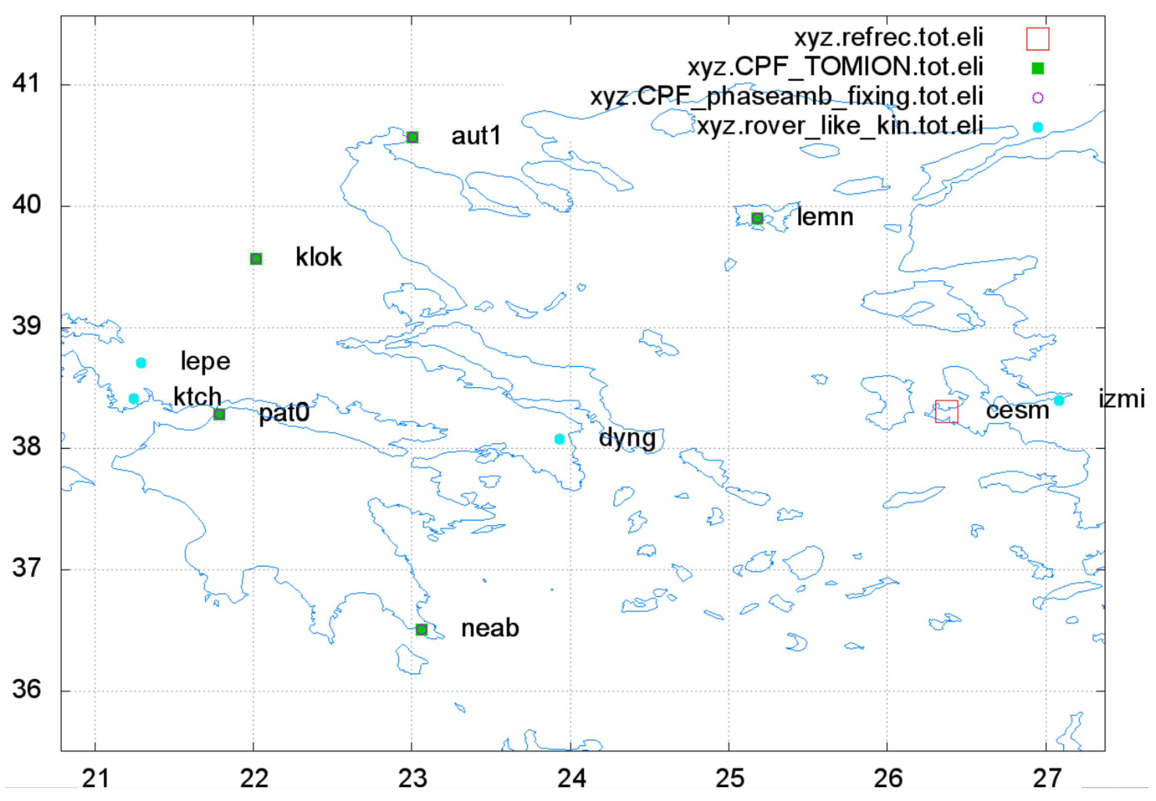
3.1. Data Set

The assessment of the WARTK corrections was carried out with data collected from NOANET GNSS network in Greece on 12 June 2018. The ionospheric-geodetic WARTK model is solved emulating real-time conditions from the GPS observations of a limited number (five) of permanent receivers: AUT1, KLOK, LEMN, NEAB and PAT0 separated a few hundreds of km; and the reference station: CESM. This separation can be as large as around 900 km between close receivers at mid latitude in an approximately uniformly distributed network (see [12]). Three additional permanent receivers were treated as rovers: LEPE, KTCH and DYNG. The locations of all GNSS receivers are shown in Figure 1.

Figure 1. GNSS receivers from NOANET GNSS network in Greece.

KLOK, LEMN and NEAB are permanent stations of NOANET GNSS Network in Greece (please refer to [13]). In addition, we have access to the CESM station of the Turkish RTK CORS network (TNPGN-Active), which complements the circular distribution of permanent GNSS receivers at more than 100 km distance from the receiver DYNG, treated as a roving user.

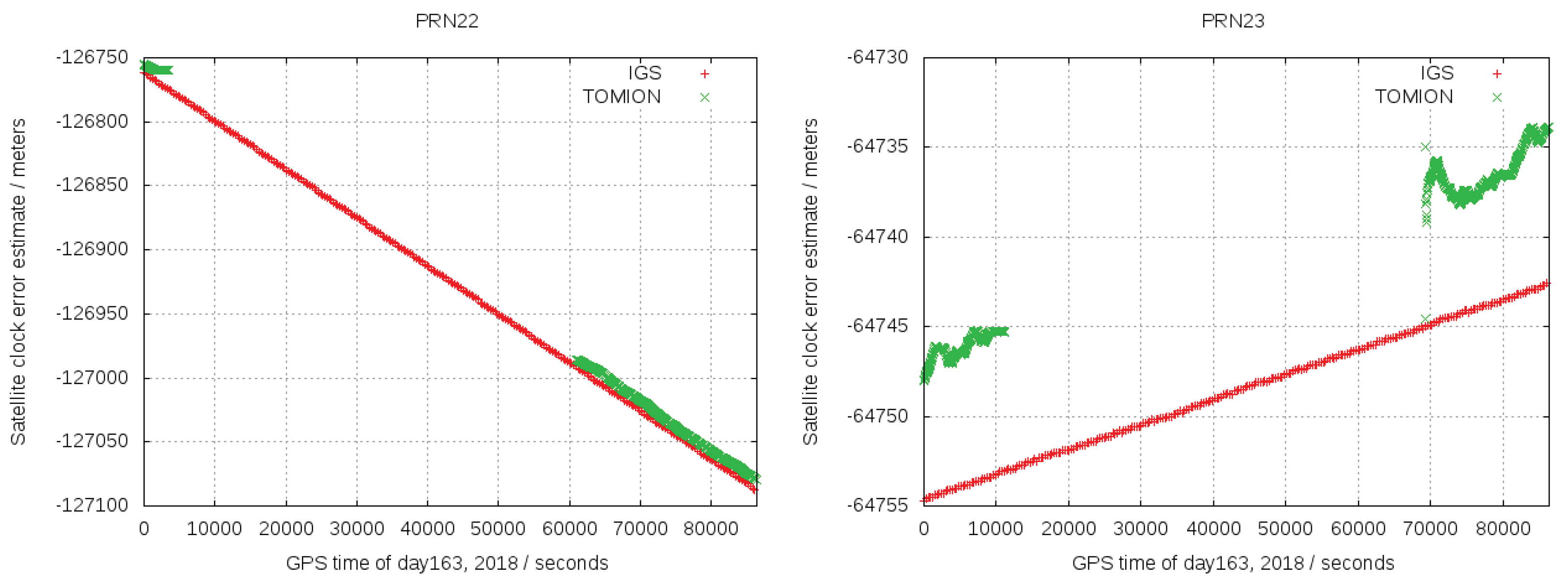
3.2. Satellite Clock Assessment

The real-time satellite clock estimates from the WARTK network were compared with the final values estimated globally by the IGS analysis centers. Figure 2 shows two typical examples of satellite clocks estimated by WARTK and IGS, green and red, respectively. It has to be noted that the WARTK solution is based on the GNSS data of the corresponding wide-area network, then providing satellite clocks estimations for each given satellite when it is in view only. Consequently, when the satellite clock error correction is needed by the roving user, then there is no need of external satellite clock estimations.The plots in Figure 2 are representative of the agreement between TOMION solutions for the WARTK model and IGS corrections, left and right plots for PRN22 and PRN23, respectively. In both cases, the clock errors show the same trend and a similar positive offset (of around 7 m for PRN23). TOMION solutions were computed by emulating real-time conditions, as opposed to the IGS final post-processed measurements, having hence a higher variability in the solutions from TOMION. Moreover, the wide-area network is not able to simultaneously observe and estimate all the satellite clock errors, differently from the global IGS network used for computing the final IGS satellite clocks, as it can be appreciated on the figure. Therefore, it was not possible to apply the same datum, and the sum of all simultaneously estimated satellite clock errors was equal to zero. This fact explained a common offset. Another reason for the differences regarding the stability of the clock errors was that the IGS network is world-wide and contains higher numbers of receivers with common satellites in view, thereby increasing the stability of these errors with respect to regional networks.

Figure 2. GPS clock errors for PRN22 (left) and PRN23 (right) from WARTK TOMION (green) and IGS (red).

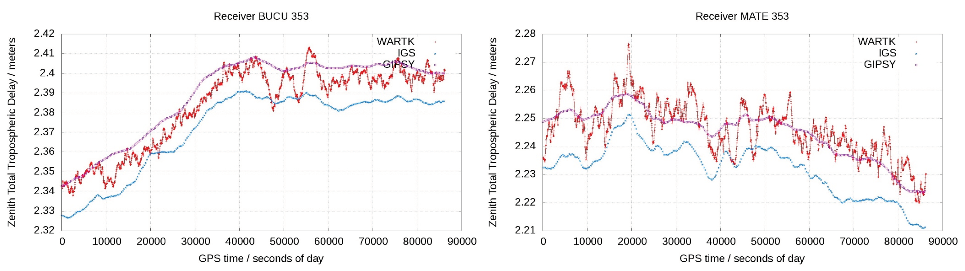
3.3. Zenith Tropospheric Delay Assessment

Another real-time positioning error source, very sensitive to the quality of the CPF processing, is the Zenith Tropospheric Delay (ZTD), estimated as random walk in the TOMION CPF filter. This assessment was carried out by using data from two IGS receivers (BUCU in Romania and MATE in Italy) close to NOANET. Figure 3 shows the ZTD computed by TOMION (red), GIPSY (see [14], magenta), and IGS (blue), for both receivers. The real-time WARTK TOMION solution was noisier for both receivers but with a positioning error of +1 cm (ca. also for next values) for BOCU and +2 cm for MATE, both with respect to the post-processed IGS solution. Similarly to the clock errors, one potential reason for such difference in stability is that IGS tropospheric products are also post-processed. However, the post-processed GIPSY solution also shows a positioning error with respect to the IGS solution of about 2 cm [15], whereas its difference with TOMION is kept lower than 1 cm for both receivers.

Figure 3. ZTD computed by WARTK TOMION (red), GIPSY (magenta) and IGS (blue) for BUCU (Romania) and MATE (Italy) GNSS receivers from IGS GNSS network.

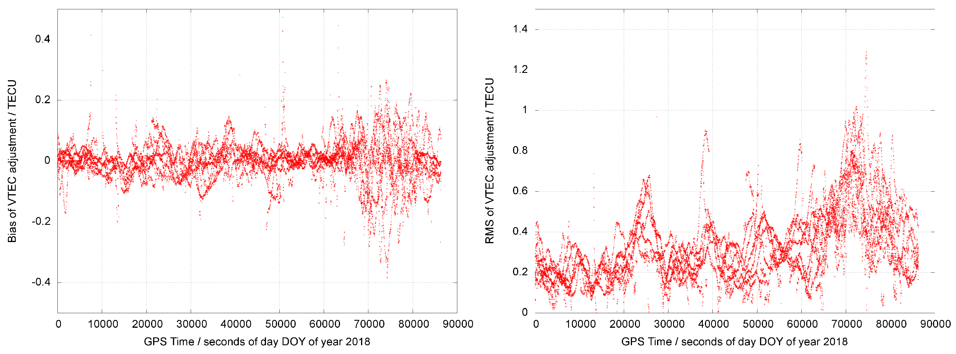
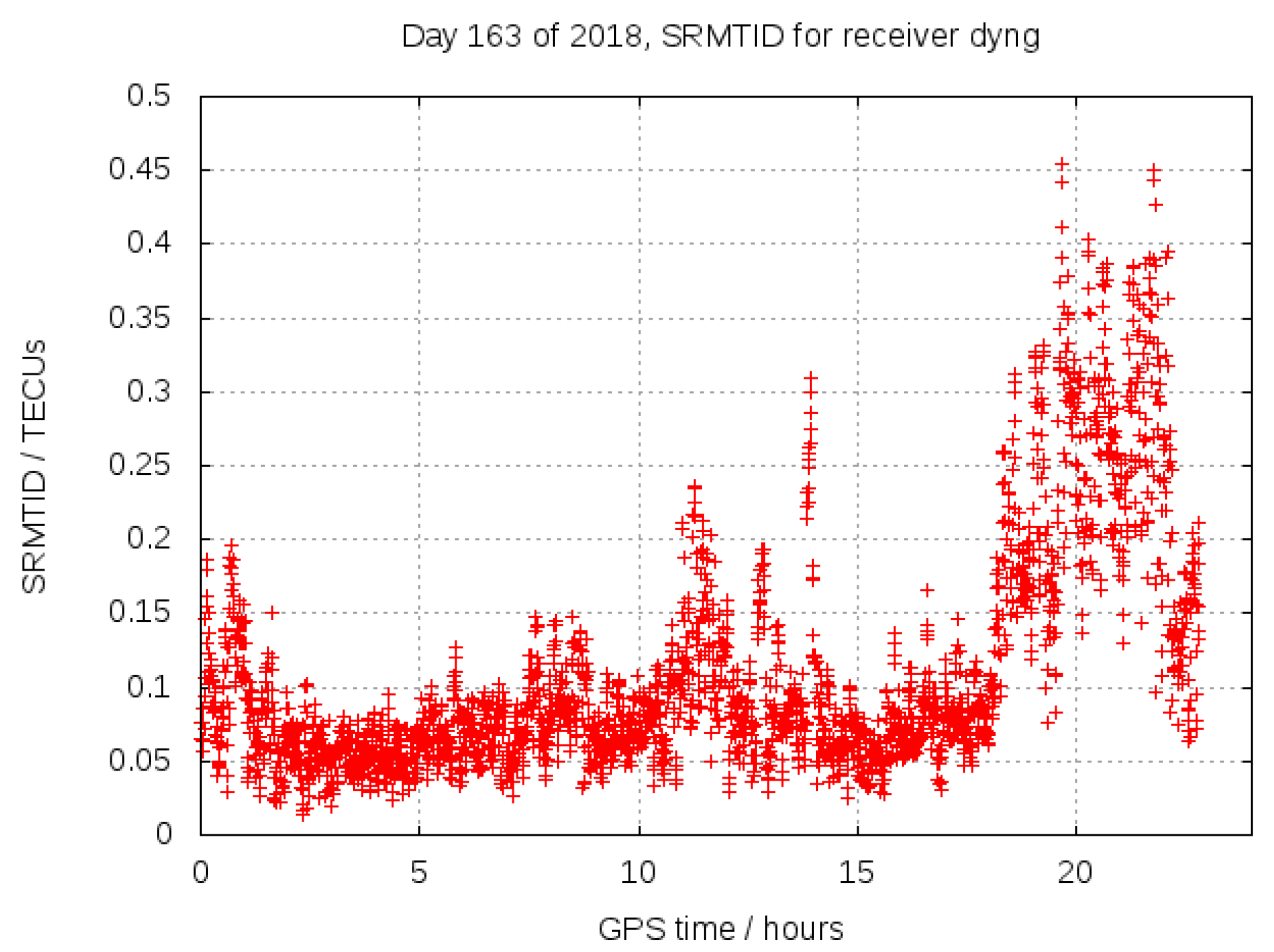
3.4. Ionospheric Corrections Assessment

TOMION ionospheric corrections were broadcast (by means of an in-house message format for corrections developed in the AUDITOR project) to the users in terms of an independent linear fit of the VTEC per satellite and epoch. They are typically distributed in the same ionospheric region and with a similar ionospheric mapping function, and the fitting is performed from the STECs determined for the permanent receivers by the WARTK model (see previous section). Once such an interpolated VTEC was computed by the user, then the STECs could be computed by means of the following formula, involving the standard ionospheric mapping function ${\left(M_I\right)}_r^s$ and the VTEC, V:

$$S_r^s={\left(M_I\right)}_r^s·V={\left[1-{\left(\frac{R_{r}cos{E}_r^s}{R_e+h}\right)}^2\right]}^{-1/2}·V,$$

(7)

where $R_e$ is the average Earth’s radius, $R_r$ is the receiver geocentric distance, h is the effective height, set up to 450 km, where all the ionospheric electron content is supposed to be located (thin-shell approach), and $E_r^s$ is the elevation angle of the satellite s above the local horizon of receiver r. For each given GNSS satellite in view, the VTEC was obtained from a linear combination of all the VTECs computed from the reference network by the CPF.

The error bias and RMS of such fitting, as well as the residuals, are shown in Figure 4 for the considered day. For the most part of the day, VTEC error bias and RMS were within $0.2TECU$ and $1TECU$, respectively. However, the results were significantly affected by Traveling Ionospheric Disturbances (TIDs) during the last hours of the day (around 70,000–80,000 s), as expected for the local spring–summer, and can be seen in terms of the Single Receiver MSTID index (SRMTID) evolution on DYNG shown in Figure 5 (see [16] for more details on SRMTID).

Figure 4. The bias (left) and RMS (right) of the residuals of the VTEC fitting per satellite (vertical axis in TECU) vs. time (horizontal axis in seconds of the day) is represented during the day 12 June 2018.

Figure 5. SRMTID index for roving receiver DYNG, versus GPS time in hours of day 12 June 2018.

4. Impact of WARTK Corrections in Navigation of Roving GNSS Users

The final WARTK assessment was focused on the analysis of the performance of the navigation solutions for GNSS receivers roving within the WARTK permanent network. WARTK provided corrections for satellite clock errors, satellite DCBs and ionospheric corrections (not for ZTD for the time being), which were then used by any rover within the network, in order to increase the positioning and navigation accuracy, as well as the convergence speed of their estimates in Equation (6), by means of the WARTK ambiguity constraint. This test was carried out in two scenarios: two fixed receivers treated as a rover (to quantify) and a real moving rover, a tractor doing spraying tasks in agriculture (to confirm). In both cases, the ambiguities were not fixed but loosely constrained (via Equation (3)), so that it was less risky, thereby avoiding sudden errors associated with biased positions. This results in a clear reduction of the convergence time and horizontal positioning error, as we will show in detail in the first scenario.

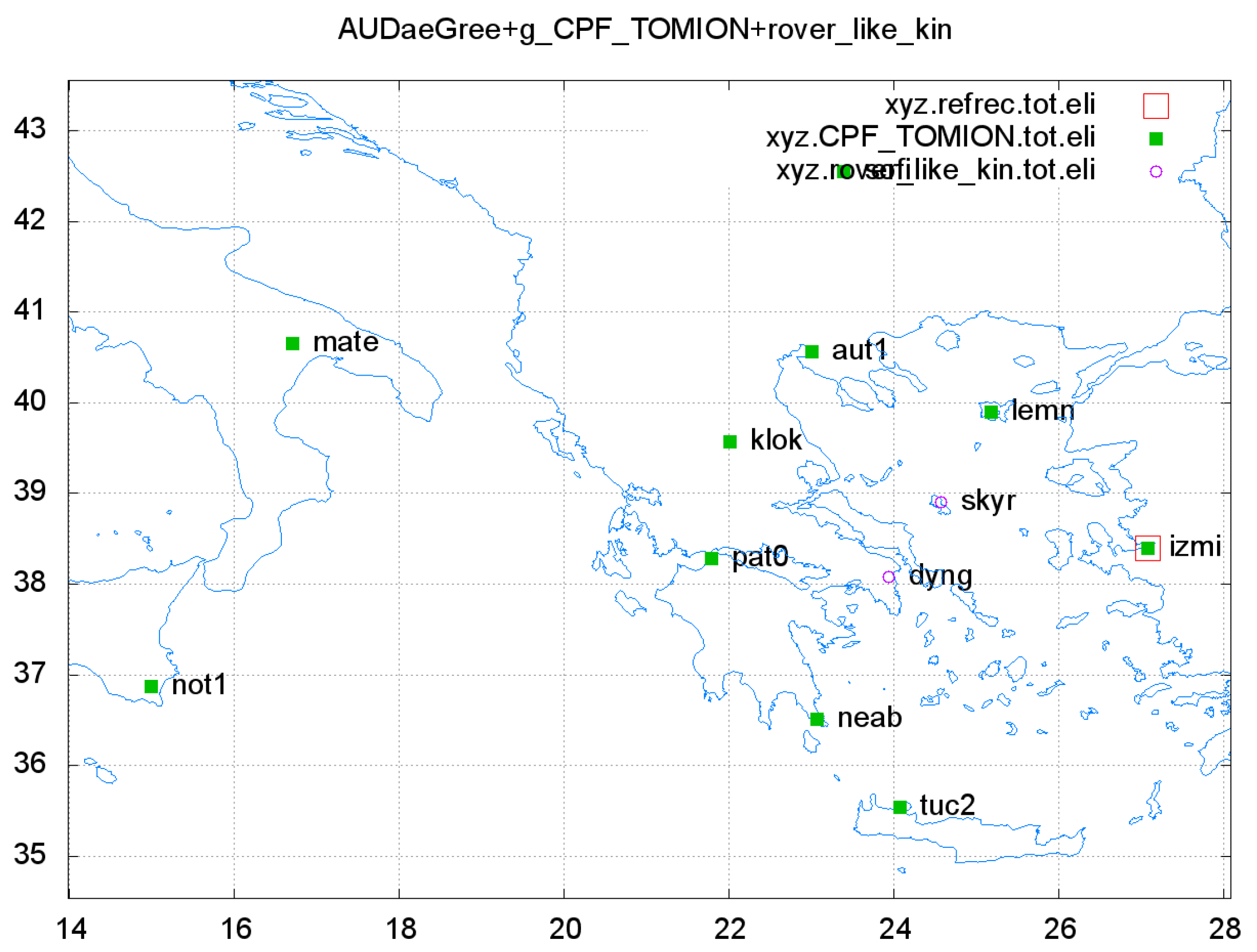
4.1. First Scenario: Static Rovers in NOANET

In order to characterize in detail the WARTK precision and convergence time, we have extended the study done in previous section from 2 to 11 days (11–21 June 2018). Moreover, we have focused on the horizontal positioning error, the one actually important for agriculture and ground applications, and on its convergence time. We have also explored different possibilities in ambiguity fixing and estimation, under a 30-second rate, to facilitate the different intensive computations.

4.1.1. Wide-Area Networks of Receivers

One main network was defined to extend the wide-area RTK study, with receivers available for the whole period: 10 permanent GPS receivers and two additional permanent ones (DYNG and SKYR) treated as roving users, switching on and off each 2 h (cold starts), and at more than 100 km and almost 200 km from the nearest permanent site, respectively (see Figure 6; and with IZMI as reference receiver).

Figure 6. The baseline network of GNSS receivers used in the extensive WARTK study since 11 to 21 June 2018, where the permanent receivers DYNG and SKYR are treated as rovers, and the permanent receiver IZMI is taken as reference for WARTK.

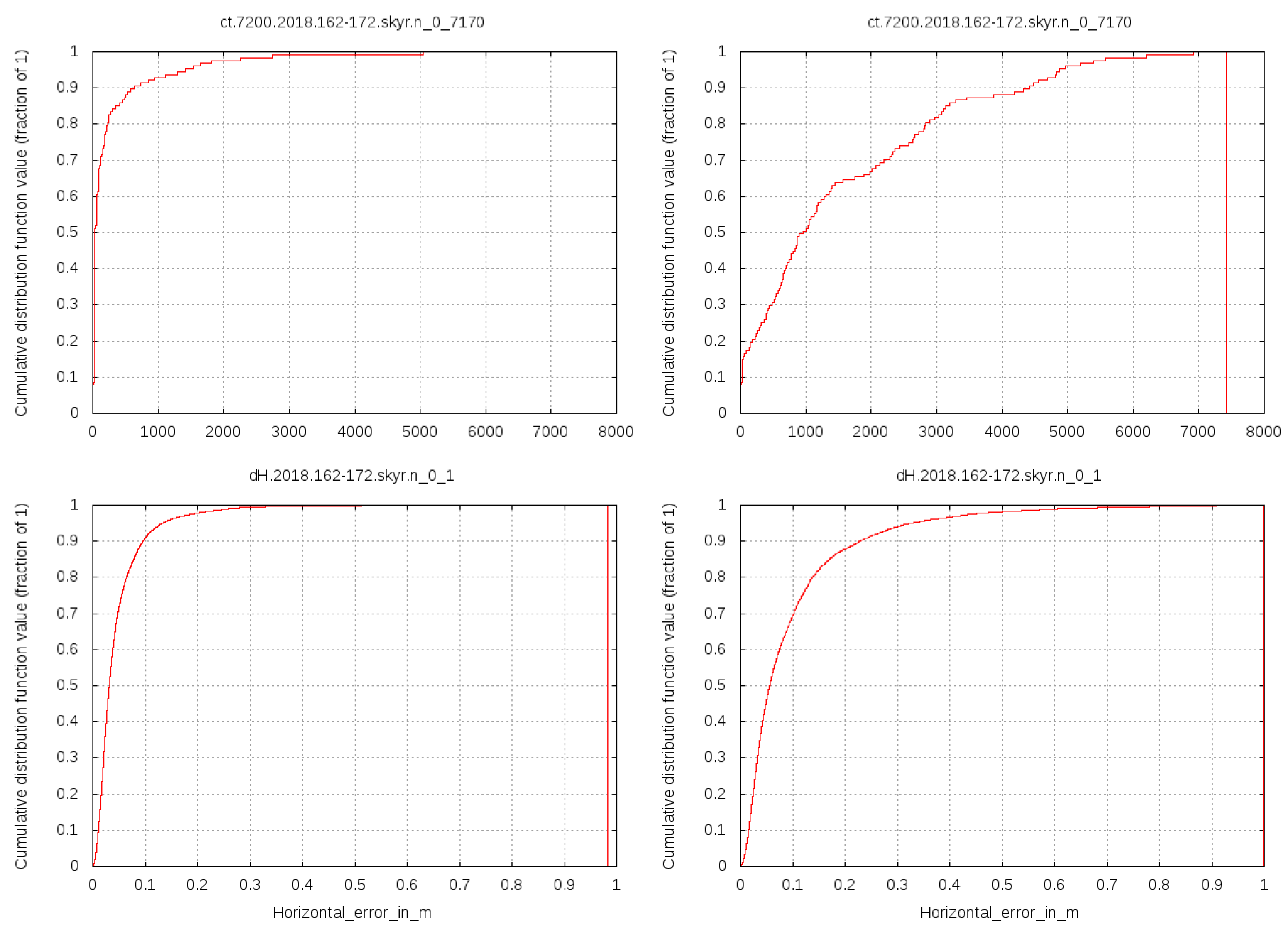
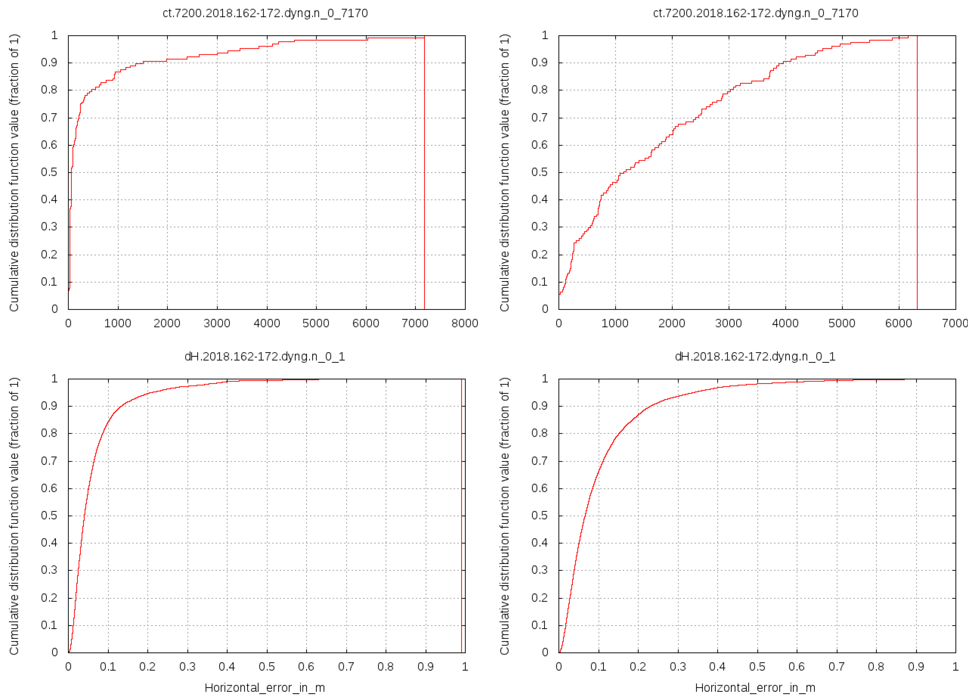
4.1.2. Convergence Time below 10 cm of Horizontal Positioning Error

Different strategies were compared in terms of convergence time and final horizontal positioning accuracy; in spite of that, we will only focus on the main ones, those representing different categories in the quality of the solution.

The convergence time is defined in this work as the time required to reach a horizontal positioning error below 10 cm. In our case, for receivers DYNG and SKYR treated as rovers, and since day 162 to 172 of year 2018, we introduced one complete cold start for both receivers every 2 h (the initial WARTK CPF convergence time during first day is also included).

Indeed, in the first row of Figure 7, the roving receiver SKYR shows convergence times for the 50%, 75% and 95% of cases equal or below 30 s (single-epoch), 150 s and 600 s approximately, vs. 1000 s, 2750 s and 4850 s without ambiguity constraining with WARTK in the same daytime scenario. A significant reduction in the horizontal real-time roving positioning error has also been confirmed (second raw of Figure 7) in spite of it being not so strong such as in the convergence time, up to more than one order of magnitude of reduction in such a case. Indeed, the real-time horizontal position errors for SKYR during the daytime are up to 3 cm, 5 cm and 12 cm for 50%, 75% and 95% of cases, respectively, by constraining and continuously updating the ambiguities without updating the permanent receiver coordinates, vs. the 6 cm, 12 cm and 32 cm, respectively, in the same conditions but without constraining the ambiguities.

Figure 7. Summary of results for roving user SKYR. First row: Percentage of cumulative cases, over the 132 roving user resets between days 162 to 172, 2018, vs. convergence time for horizontal positioning error, in seconds. Second row: Corresponding final horizontal positioning error, in meters. First column: WARTK, constraining ambiguities updating them at every chance, and slightly estimating the permanent receivers coordinates; second column: no ambiguity constraining (i.e., without using the WARTK ionospheric corrections).

The results obtained with WARTK on DYNG are quite similar, just slightly worse than the ones for SKYR. This is coinciding with the almost double of distance (more than 200 km) of this roving user to the nearest reference site (see Figure 6). Indeed it can be seen in top-left plot of Figure 8 a convergence time smaller than 75 s for 50% of 132 cold user starts, each 2 h in 11 days, smaller than 250 s for 75% of the cases and smaller than 3400 s for the 95% of the cases approximately. When no ionospheric correction and hence no ambiguity constraint is applied (top-right plot of Figure 8), the convergence time is slightly smaller than 1100 s for 50% of cold user starts, smaller than 2700 s for 75% of the cases and smaller than 4600 s for 95% of the cases approximately.

Figure 8. Summary of results for roving user DYNG. First row: Percentage of cumulative cases, over the 132 roving user resets between days 162 to 172, 2018, vs. convergence time for horizontal positioning error, in seconds. Second row: Corresponding final horizontal positioning error, in meters. First column: WARTK constraining ambiguities, updating them at every chance; second column: no ambiguity constraining.

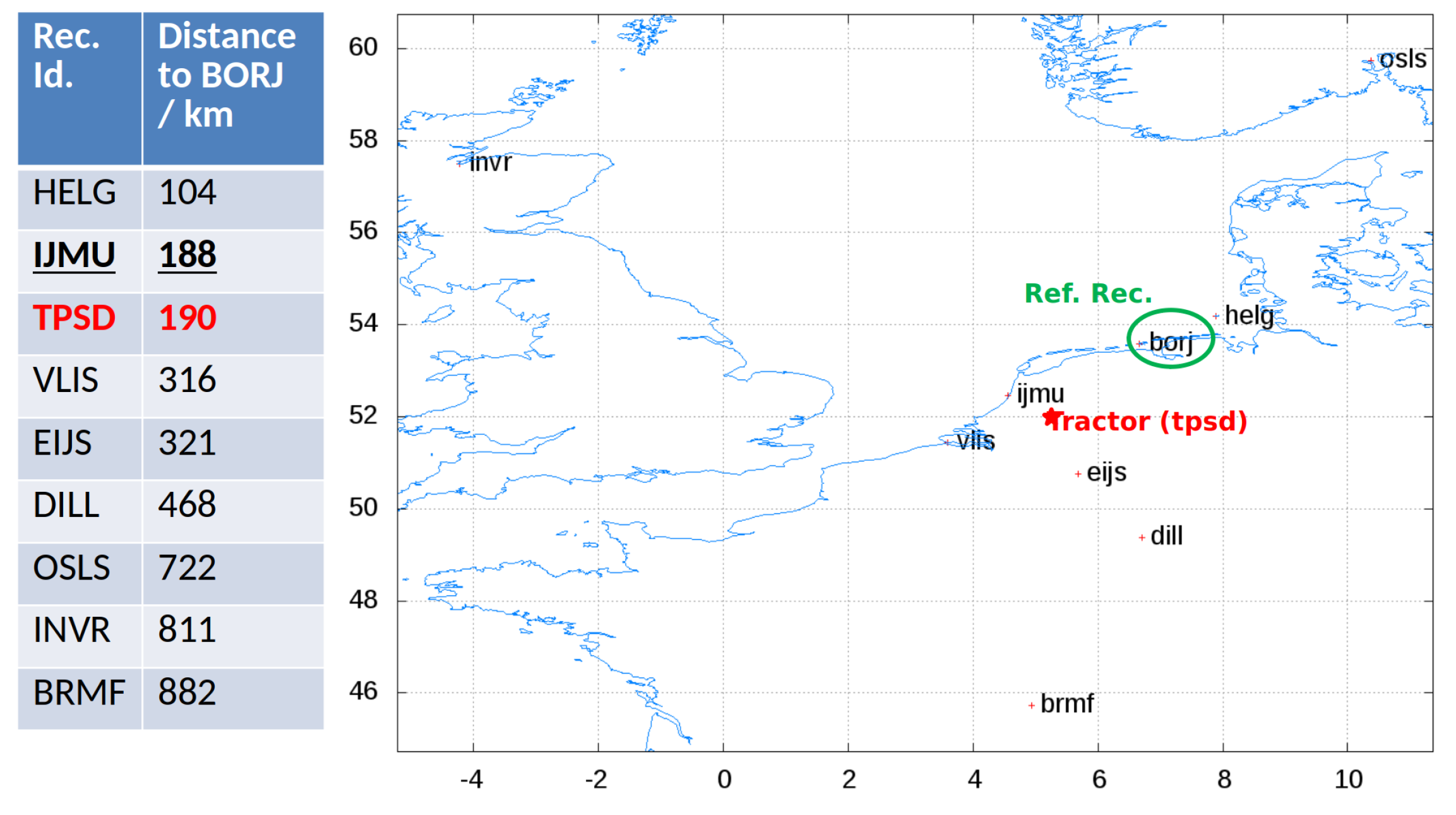
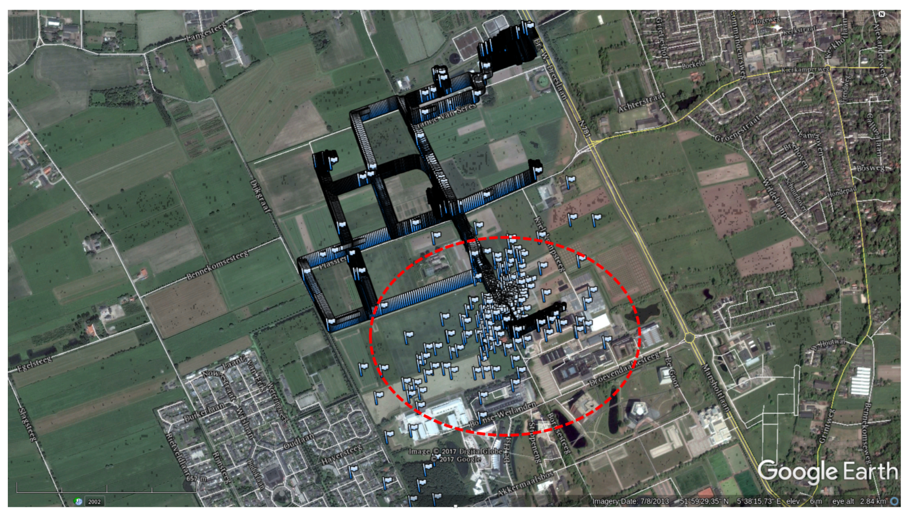
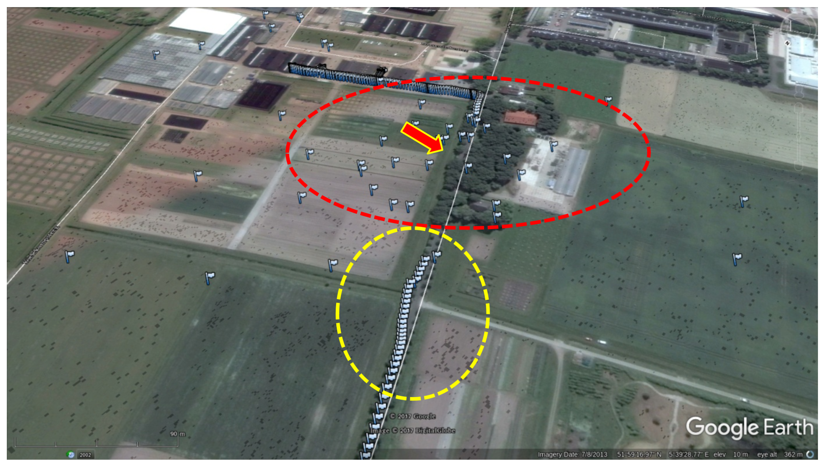
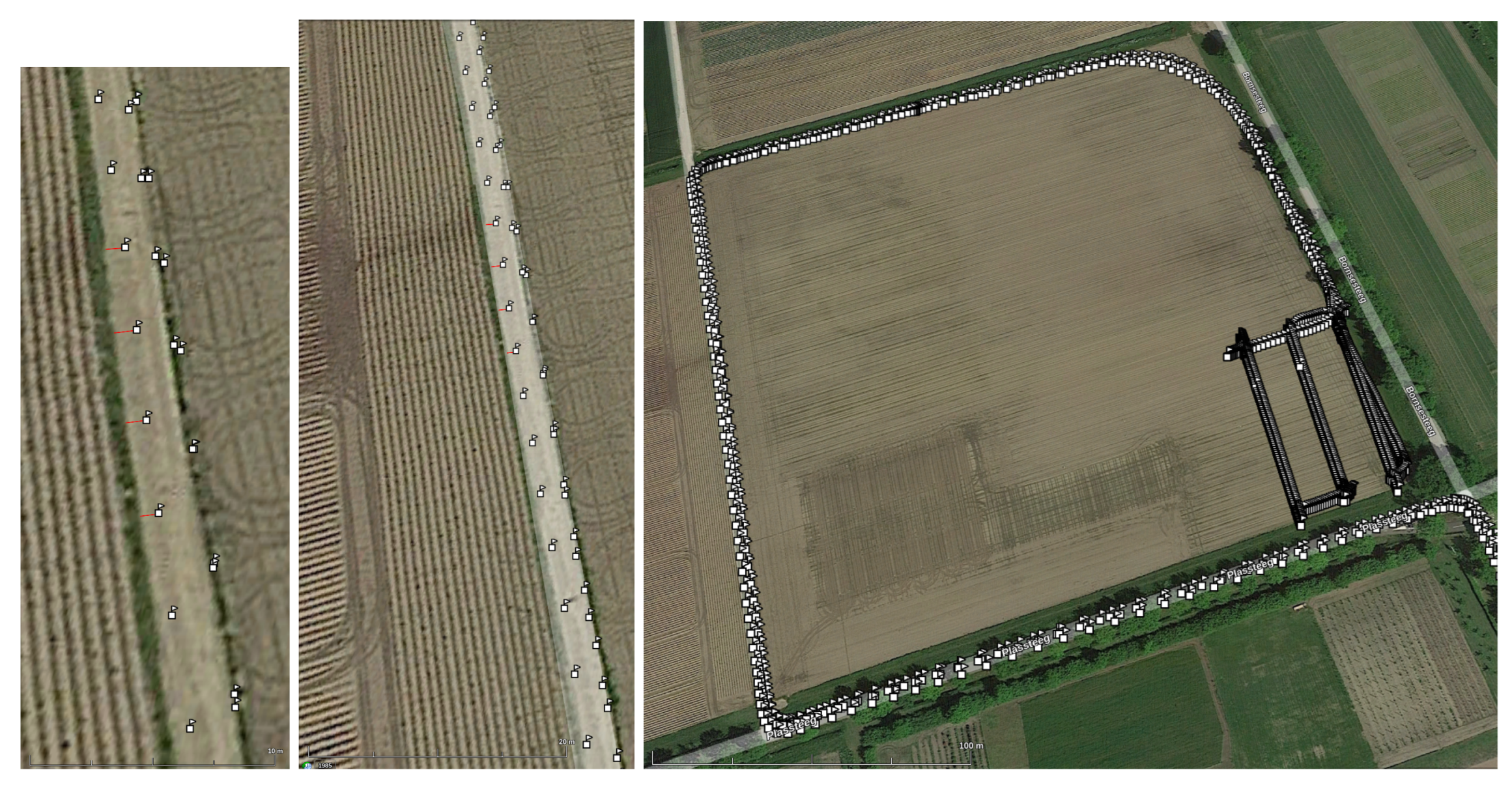
4.2. Second Scenario: Spraying Tractor Mounted Rover

A real kinematic case was also considered to show the impact of external WARTK corrections in high-accuracy positioning and navigation, consistently with the detailed characterization of the convergence time and horizontal accuracy studied, summarized in the previous section. The test was carried out by using a spraying tractor for agriculture applications at an experimental farm of the Wageningen University (WUR), the Netherlands, for the day 164 (13 of June) of year 2017. The GPS measurements, gathered by a TOPCON GP-DX1 GNSS receiver, were processed with TOMION at 1 Hz emulating WARTK real-time conditions, with reference receiver BORJ and seven additional permanent receivers (see Figure 9).

Figure 9. Right: Figure containing the location of the spraying tractor (TPSD) vs. the reference (BORJ) and permanent WARTK receivers (the remaining ones, excepting IJMU); Left: the table of distances to BORJ.

We can see in Figure 10 the overall trajectory at 1 Hz provided by TOMION emulating WARTK in real-time (RT) conditions, during the almost 7 h of work, showing two clearly different regions: the one at the bottom (inside the red ellipse) where the positioning error is huge, associated to the existing dense canopy and consequent huge number of cycle-slips; and the remaining part (most part of the trajectory), well aligned with the existing paths.

Figure 10. Trajectory obtained with WARTK for the spraying tractor TPSD during the whole agriculture activity (from 06 h 11 m to 13 h, day 164, 2017).

The dense canopy (see red arrow in Figure 11) has provided us the opportunity to observe, right afterwards, the convergence time of the actual WARTK roving user in emulated RT conditions. Indeed, as can be seen in Figure 11, a total of around 20 one-hertz consecutive epochs are needed to get the positioning fully consistent with the path (within the yellow ellipse) right after leaving the canopy. This time of around 20 s is in full agreement with the WARTK results quantified in the previous scenario (for instance for SKYR).

Figure 11. Detail of TPSD WARTK trajectory: convergence (under yellow ellipse) of the rover position after leaving the canopy (red ellipse).

The same experiment, thanks to the georeference provided by the map, gives us as well the opportunity to directly observe the precision, and likely the accuracy due to the well fitting on the way, by comparing consecutive positions with the border of the path. Indeed, in Figure 12, in a part of the track far from the canopy, it can be seen a distance to the path border varying at the level or below the decimeter, consistently with the accuracy quantified in the previous scenario.

Figure 12. Detail of TPSD WARTK trajectory, showing (with a zoom from the right to the left) the consistency of the tractor distance to the path border (representative red segments at the left-hand plot with lengths of 97 cm, 96 cm, 91 cm and 83 cm) with the expected WARTK accuracy at decimeter level.

5. Conclusions

This paper has introduced the WARTK equations for the network (CPF) and the rover. The CPF provides corrections for satellite clocks and DCBs, as well as ionospheric corrections that then any rover within the network can use to increase the convergence time and accuracy in precise positioning and navigation. In order to assess the quality of the corrections, it was possible to compare the satellite clock errors and ZTD computed, emulating real-time conditions with their counterparts computed by IGS from global data and in post-processing mode. The difference between satellite clocks from WARTK and IGS results in being biased within the GPS constellation, as the different datum of addition of simultaneously estimated satellite clock errors is constantly equal to zero. Moreover, the difference between WARTK and GIPSY ZTD corrections was found within 1 cm, whereas the IGS ZTD product was up to 2–3 cm away from the two formers. The assessment on the ionospheric corrections was carried out through the comparison of the correction with the observed VTEC for each satellite in view. Differences resulted within $0.2TECU$, and the RMS error is usually much lower than 1 m. However, at the end of the day, it has been observed that the seasonal activity of TIDs may increase the positioning error and the RMS higher than the aforementioned values. Finally, we have presented the results of using the WARTK corrections computed by the CPF in two scenarios in the Mediterranean basin: Greece and the Netherlands. The results of the field test carried out in Greece showed that the ionospheric corrections reduces the convergence time to achieve horizontal positioning errors below 10 cm up to 30 s (single-epoch), 150 s and 600 s for the 50%, 75% and 95% of cases, in front of 1000 s, 2750 s and 4850 s without ionospheric corrections, respectively. Furthermore, this experiment also showed the horizontal accuracy of the kinematic solutions reached up to 3 cm, 5 cm and 12 cm with WARTK for the 50%, 75% and 95% of cases in front of 6 cm, 12 cm and 32 cm without, affected all of them by the MSTIDs occurrence. The second test carried out in the Netherlands assessed the performance of the WARTK corrections through the observations of the kinematic solution consistency for the spraying tractor mounted rover with the georeference provided by the map and the cold-starts produced by the canopy. Both solutions achieved a positioning error at decimeter level, with a convergence time of few tens of seconds, consistently with the results in the first scenario of Greece. Although the WARTK model proved to perform well for kinematic users in sparse networks, in order to achieve, at any time after few observation epochs, decimeter error level accuracy in positioning and navigation, it is also necessary to implement algorithms for mitigation of the impact of MSTIDs [17,18].

References

- Hernández-Pajares, M.; Juan, J.; Sanz, J.; Colombo, O.L. Application of ionospheric tomography to real-time GPS carrier-phase ambiguities Resolution, at scales of 400–1000 km and with high geomagnetic activity. Geophys. Res. Lett. 2000, 27, 2009–2012. [Google Scholar] [CrossRef]
- Zumberge, J.; Heflin, M.; Jefferson, D.; Watkins, M.; Webb, F. Precise point positioning for the efficient and robust analysis of GPS data from large networks. J. Geophys. Res. 1997, 102, 5005–5017. [Google Scholar] [CrossRef]
- Olivares-Pulido, G.; Terkildsen, M.; Arsov, K.; Teunissen, P.; Khodabandeh, A.; Janssen, V. A 4 D tomographic ionospheric model to support PPP-RTK. J. Geod. 2019, 93, 1673–1683. [Google Scholar] [CrossRef]
- Olivares-Pulido, G.; Hernández-Pajares, M.; Lyu, H.; Gu, S.; García-Rigo, A.; Graffigna, V.; Tomaszewski, D.; Wielgosz, P.; Rapiński, J.; Krypia-Gregorczyk, A.; et al. Ionospheric tomographic common clock model of undifferenced uncombined GNSS measurements. J. Geod. 2021, 95, 122. [Google Scholar] [CrossRef]
- Teunissen, P.; Khodabandeh, A. Review and principles of PPP-RTK methods. J. Geod. 2015, 89, 217–240. [Google Scholar] [CrossRef]
- Odijk, D.; Khodabandeh, A.; Nadarajah, N.; Choudhury, M.; Zhang, B.; Li, W.; Teunissen, P.J. PPP-RTK by means of S-system theory: Australian network and user demonstration. J. Spat. Sci. 2017, 62, 3–27. [Google Scholar] [CrossRef]
- Teunissen, P.; Montenbruck, O. Springer Handbook of Global Navigation Satellite Systems; Springer: Berlin/Heidelberg, Germany, 2017; p. 1327. [Google Scholar] [CrossRef]
- Hernández-Pajares, M.; Aragón-Ángel, À.; Defraigne, P.; Bergeot, N.; Prieto-Cerdeira, R.; García-Rigo, A. Distribution and mitigation of higher-order ionospheric effects on precise GNSS processing. J. Geophys. Res. Solid Earth 2014, 119, 3823–3837. [Google Scholar] [CrossRef]
- Hernandez-Pajares, M.; Juan, J.; Sanz, J. Neural network modeling of the ionospheric electron content at global scale using GPS data. Radio Sci. 1997, 32, 1081–1089. [Google Scholar] [CrossRef]
- Hernández-Pajares, M.; Juan, J.; Sanz, J. New approaches in global ionospheric determination using ground GPS data. J. Atmos. Sol.-Terr. Phys. 1999, 61, 1237–1247. [Google Scholar] [CrossRef]
- Boehm, J.; Schuh, H. Vienna mapping functions in VLBI analyses. Geophys. Res. Lett. 2004, 31. [Google Scholar] [CrossRef]
- Hernández-Pajares, M.; Juan, J.; Sanz, J.; Aragon-Angel, A.; Ramos-Bosch, P.; Samson, J.; Tossaint, M.; Albertazzi, M.; Odijk, D.; Teunissen, P.; et al. Wide-area RTK: High precision positioning on a continental scale. Inside GNSS 2010, 5, 35–46. [Google Scholar]
- Ganas, A.; Drakatos, G.; Rontogianni, S.; Tsimi, C.; Petrou, P.; Papanikolaou, M.; Argyrakis, P.; Boukouras, K.; Melis, N.; Stavrakakis, G. NOANET: The new permanent GPS network for Geodynamics in Greece. Geophys. Res. Abstr. 2008, 10, 1. [Google Scholar]
- Bertiger, W.; Bar-Sever, Y.; Dorsey, A.; Haines, B.; Harvey, N.; Hemberger, D.; Heflin, M.; Lu, W.; Miller, M.; Moore, A.W.; et al. GipsyX/RTGx, a new tool set for space geodetic operations and research. Adv. Space Res. 2020, 66, 469–489. [Google Scholar] [CrossRef]
- Graffigna, V. Consistency of Different Tropospheric Models and Mapping Functions for Precise GNSS Processing. Master’s Thesis, Universitat Politècnica de Catalunya, Barcelona, Spain, 2017. [Google Scholar]
- Hernández-Pajares, M.; Juan, J.; Sanz, J.; Aragón-Àngel, A. Propagation of medium scale traveling ionospheric disturbances at different latitudes and solar cycle conditions. Radio Sci. 2012, 47, 1–22. [Google Scholar] [CrossRef]
- Hernández-Pajares, M.; Wielgosz, P.; Paziewski, J.; Krypiak-Gregorczyk, A.; Krukowska, M.; Stepniak, K.; Kaplon, J.; Hadas, T.; Sosnica, K.; Bosy, J.; et al. Direct MSTID mitigation in precise GPS processing. Radio Sci. 2017, 52, 321–337. [Google Scholar] [CrossRef]
- Yang, H.; Monte-Moreno, E.; Hernández-Pajares, M. Multi-TID detection and characterization in a dense GNSS receiver network. J. Geophys.Res. Space Phys. 2017, 122, 9554–9575. [Google Scholar] [CrossRef]
Publisher’s Note: MDPI stays neutral with regard to jurisdictional claims in published maps and institutional affiliations. |
© 2022 by the authors. Licensee MDPI, Basel, Switzerland. This article is an open access article distributed under the terms and conditions of the Creative Commons Attribution (CC BY) license (https://creativecommons.org/licenses/by/4.0/).
Share and Cite
Hernández-Pajares, M.; Olivares-Pulido, G.; Graffigna, V.; García-Rigo, A.; Lyu, H.; Roma-Dollase, D.; de Lacy, M.C.; Fernández-Prades, C.; Arribas, J.; Majoral, M.; et al. Wide-Area GNSS Corrections for Precise Positioning and Navigation in Agriculture. Remote Sens. 2022, 14, 3845. https://doi.org/10.3390/rs14163845
Hernández-Pajares M, Olivares-Pulido G, Graffigna V, García-Rigo A, Lyu H, Roma-Dollase D, de Lacy MC, Fernández-Prades C, Arribas J, Majoral M, et al. Wide-Area GNSS Corrections for Precise Positioning and Navigation in Agriculture. Remote Sensing. 2022; 14(16):3845. https://doi.org/10.3390/rs14163845
Chicago/Turabian StyleHernández-Pajares, Manuel, Germán Olivares-Pulido, Victoria Graffigna, Alberto García-Rigo, Haixia Lyu, David Roma-Dollase, M. Clara de Lacy, Carles Fernández-Prades, Javier Arribas, Marc Majoral, and et al. 2022. "Wide-Area GNSS Corrections for Precise Positioning and Navigation in Agriculture" Remote Sensing 14, no. 16: 3845. https://doi.org/10.3390/rs14163845
APA StyleHernández-Pajares, M., Olivares-Pulido, G., Graffigna, V., García-Rigo, A., Lyu, H., Roma-Dollase, D., de Lacy, M. C., Fernández-Prades, C., Arribas, J., Majoral, M., Tisropoulos, Z., Stamatelopoulos, P., Symeonidou, M., Schmidt, M., Goss, A., Erdogan, E., van Evert, F. K., Blok, P. M., Grosso, J., ... Hriscu, A. (2022). Wide-Area GNSS Corrections for Precise Positioning and Navigation in Agriculture. Remote Sensing, 14(16), 3845. https://doi.org/10.3390/rs14163845