LiDAR Reveals the Process of Vision-Mediated Predator–Prey Relationships

Abstract

Exploring the processes of interspecific relationships is crucial to understanding the mechanisms of biodiversity maintenance. Visually detecting interspecies relationships of large mammals is limited by the reconstruction accuracy of the environmental structure and the timely detection of animal behavior. Hence, we used backpack laser scanning (BLS) to reconstruct the high-resolution three-dimensional environmental structure to simulate the process of a predator approaching its prey, indicating that predator tigers would reduce their visibility by changing their behavior. Wild boars will nibble off about 5m of branches around the nest in order to create better visibility around the nest, adopting an anti-predation strategy to detect possible predators in advance. Our study not only points out how predator–prey relationships are affected by visibility as the environment mediates it, but also provides an operable framework for exploring interspecific relationships from a more complex dimension. Finally, this study provides a new perspective for exploring the mechanisms of biodiversity maintenance.

1. Introduction

A rising body of evidence supports the effects of direct and indirect species interactions on biodiversity [1,2,3,4,5], which are critical mechanisms for biodiversity maintenance [6,7,8,9,10]. Almost all species interactions research is based on non-process observational data or is completely simulated by models [3,11,12]. Several studies have made an attempt to explore the process of interaction, such as how landscape heterogeneity influences species dispersal, which affects species coexistence and ultimately community diversity [13]. This suggests a need for empirical testing of species interactions based on process data to advance the understanding of how they affect biodiversity. Unfortunately, we know little about how this process happens at spatial-temporal scales and what factors determine or dominate the process.

Predator–prey interactions have been extensively researched to better understand species relations [4,14,15]. Extensive literature has used changes in population indexes to characterize the effects of interspecific interactions [16]. Population indexes perform well in describing interspecific relationships on temporal scales. However, result-oriented changes in population indexes can be radical for interactions on a fine scale. Key environmental features play important roles in species interactions as they emerge and even determine this process [17,18,19]. The majority of existing research is focused on a broad two-dimensional landscape, which helps us to better comprehend the process of species interactions. Environmental features, on the other hand, operate on a much finer scale and may be more precise in revealing the process of species interactions [20]. For example, in contrast to significant spatial avoidance [21], the primary anti-predation strategy of wild dogs (Lycaon pictus) is to select fine-scale environmental features that can provide good shelter and evade detection by lions (Panthera leo) [22]. Feedbacks between extremely fine-scale data and prey–predation interactions may elucidate the game strategy of predation and anti-predation, but quantitative data are scarce. Therefore, process-oriented predator–prey interactions need to be revealed on a fine scale to assist in the elucidation of this largely uncharted but exciting aspect of community ecology.

The core behaviors of a predator–prey interaction are concealment and exposure [23,24,25], which are emergent properties of the tradeoff behavior in predation and anti-predation interactions, especially for large terrestrial mammals with vision [26,27]; indeed, this challenges us to quantify changes in visibility. The lack of an objective method makes it difficult to quantify vision because visual-based environmental heterogeneity changes are continuous and occur on a three-dimensional (3D) fine scale [28]. The emerging approach of LiDAR (light detection and ranging) can measure the 3D environmental structure at a high resolution, allowing the 3D structure of forest stands to be represented in great detail [29,30]. This technical attribute of LiDAR meets the fundamental need for quantified vision. LiDAR data can be used to explore the vision-based game strategy of predation and anti-predation in a fine-scale 3D forest.

Here, we present results from process-oriented predator–prey relationships at a fine-scale forest to investigate the effects of forest structure on animal vision, which mediates predator–prey interspecific relationships.

2. Materials and Methods

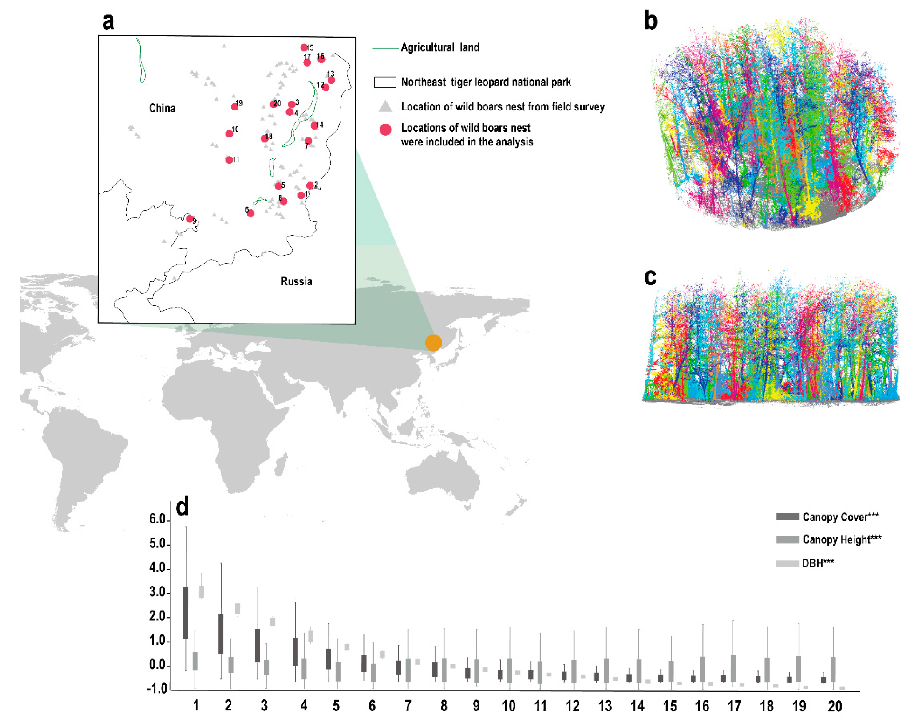
2.1. Study Area

In northeast China, the Amur tiger (Panthera tigris altaica) feeds primarily on wild boar (Sus scrofa) [31,32]. As a structural modifier [33], wild boar builds a nest for neonatal survival [34] and to reduce thermal losses (Video S1). From April to November 2020, a total of 241 wild boar nests were found in an area of 6501 km² (130.165609°E–131.317653°E and 42.614041°N–43.553505°N) (Figure 1), all of which followed the same pattern: the material for building the nest was obtained by biting off the bushes around the nest (Figure 1, Video S1). This pattern is perplexing; when wild boars use the nest, they also choose to aggressively expose themselves, increasing the risk of predation by the Amur tiger, which prefers to be as close to the prey as possible through ambush behavior to enhance prey ‘catchability’ [35]. The Amur tiger–wild boar relationship is a typical predation and anti-predation interaction dependent on vision. The primary game strategy is concealment and detection of each other, which is mediated by the 3D forest structure. Therefore, the interaction between a tiger and wild boar around the nest is an ideal model system for studying the effects of the 3D forest structure on animal vision, which mediates interspecific relationships of predator and prey. As such, we hypothesized that a tiger could reduce its visibility through ambush as a predation strategy, coming as close to the prey as possible to enhance prey ‘catchability’. However, wild boars have to use or modify the 3D forest structure around the nest as an anti-predation strategy to reduce ‘catchability’.

The 3D forest structure data acquisition at the nest scale is the key for this study. Taking the nest site as the center of an area with a radius of 25 m, the 3D forest structure data were obtained by backpack laser scanning (BLS) (Green Valley, LiBackpack 50) from 20 nests (Figure 1, Tables S1 and S2). We randomly assigned the nest selection from 241 nest sites (Table S3), while the high environmental heterogeneity of the forest was considered in the selection of nest sites to increase the robustness of the results (Table S4). Analysis of traditional forest structure traits (canopy cover, canopy height, and diameter at breast height) indicated that the forest structures of 20 nests were highly heterogeneous (analysis of K-W test, p < 0.05, Figure 1, Table S4). In a subsequent analysis, we quantified the visibility based on the 3D forest structure data.

2.2. Data Collection

2.2.1. Location Data of Wild Boar Nests

The study area was divided into 500 × 500 m grids and investigated grid by grid. Once a wild boar’s nest was found, rangers recorded the location with a global positioning system (GPS) (Table S3) and took a picture of the nest. This work provided us with 241 boar nesting sites (Figure 2a). The 241 nests were made up of 84 nests built in 2020, and 157 nests built before 2020 (Table S3). Nests in 2020 had branches with leaves, and nests before 2020 had no branches with leaves. Before 2020, the structure of the environment around the nest may have changed due to plant growth. Thus, we collected point cloud data from 20 nests randomly selected from 84 nests in 2020 (Table S1).

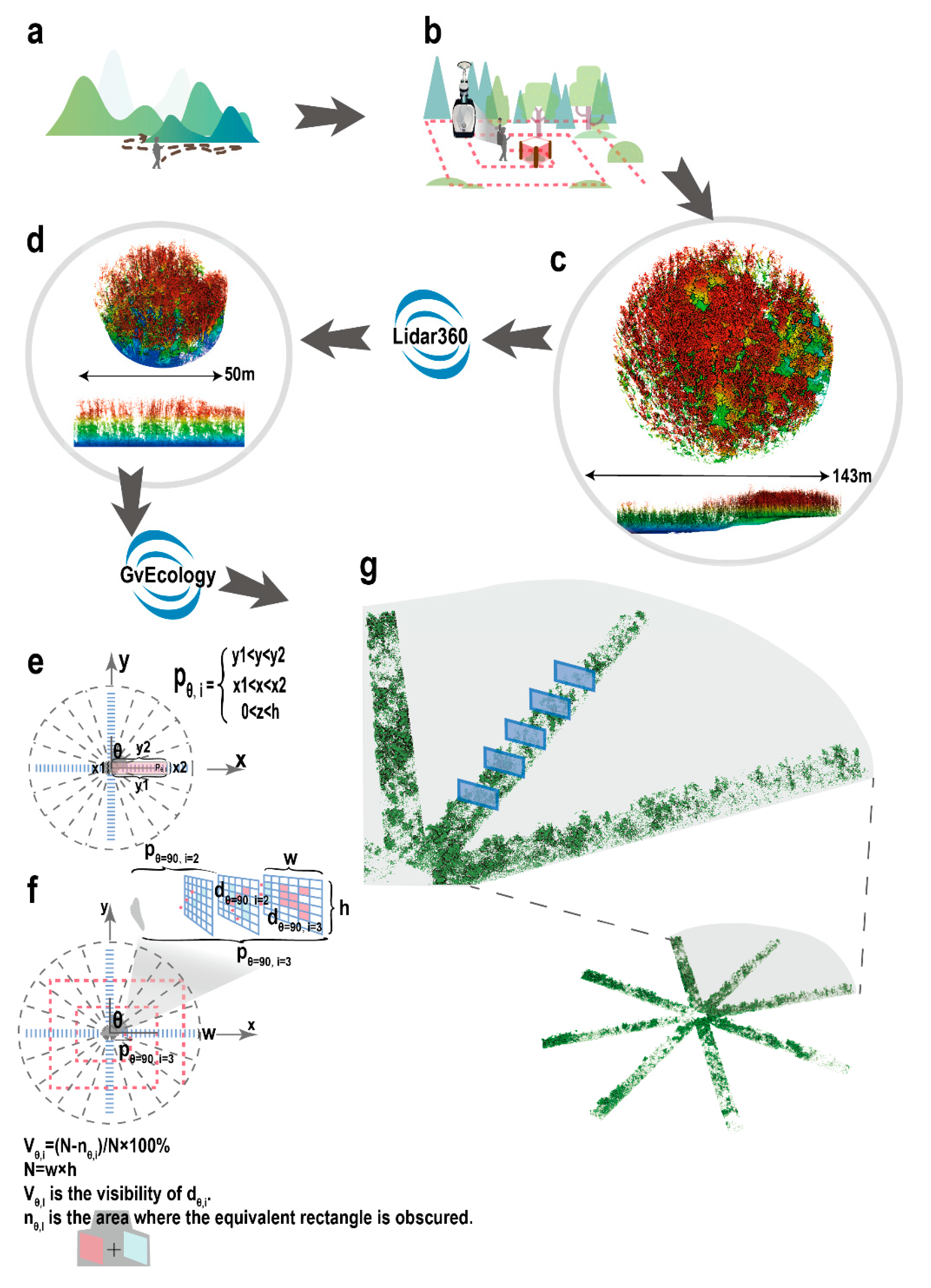
2.2.2. Point Cloud Data of the Environment Surrounding the Wild Boar Nests

We set a circular sample with a radius of 25 m around each nest (Tables S1 and S2). To make the location of the nest easier to visually identify in the massive point cloud data, we set up eye-catching fences at the nest location (Figure 2b). The fences consisted of four sides, each measuring 0.5 m high and 1.5 m long, covered with reflective stickers. Reflective stickers have higher reflective intensity, and when visualized in the form of point clouds, they are starkly different from the surrounding objects, making them easy to read visually. Within the sample, we collected environmental data using backpack laser scanning (Green Valley, LiBackpack 50), and followed the trajectory (Figure 2b). The difference is that the spiral expands outward according to a curved trajectory, while we expand outward according to a rectangular trajectory. With this trajectory, we were able to collect point cloud data covering a larger surface area of the target object horizontally. Then, we obtained fine point cloud data that could characterize the understory structure [36,37]. The BLS data were collected from 2 m above ground level, using a scan angle of 360° (horizontal) ± 15° (vertical). The BLS velocity was 1–2 m/s using the VLP-16 sensor (300,000 pts/s), resulting in an average accuracy of ±3 cm. The BLS data provided 3D vegetation structure at <3 cm spatial resolution. The only function of the fence was to effectively read the location of the nest in the big point cloud data to avoid the identification error of the location of the nest. In the subsequent analysis, the point cloud representing the fence was deleted to restore the real environmental point cloud.

2.3. Data Processing

2.3.1. Point Cloud Data Pre-Processing

After obtaining the point cloud data of the environment around 20 nests, we distinguished the ground point cloud, and used the ground point cloud to normalize the environmental point cloud, so that the lowest point cloud of the environment was at the same horizontal height (Figure 2c,d). Next, we identified the location of the nest through visual interpretation, deleted the point cloud representing the fence, and restored the real environmental point cloud. The scanning distance of BLS can reach 100 m, which means that the range of point cloud data obtained exceeded the sample range. Therefore, we cut the pre-processed point cloud data into a circular area with a radius of 25 m centered on the nest. After pre-processing, we obtained the point cloud data of 20 samples with the same range and lowest point in the same horizontal height (Figure 2d). This pre-processing was based on GreenValley Suite V5.0 (www.lidar360.com) (accessed on 15 July 2021).

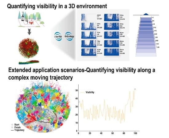
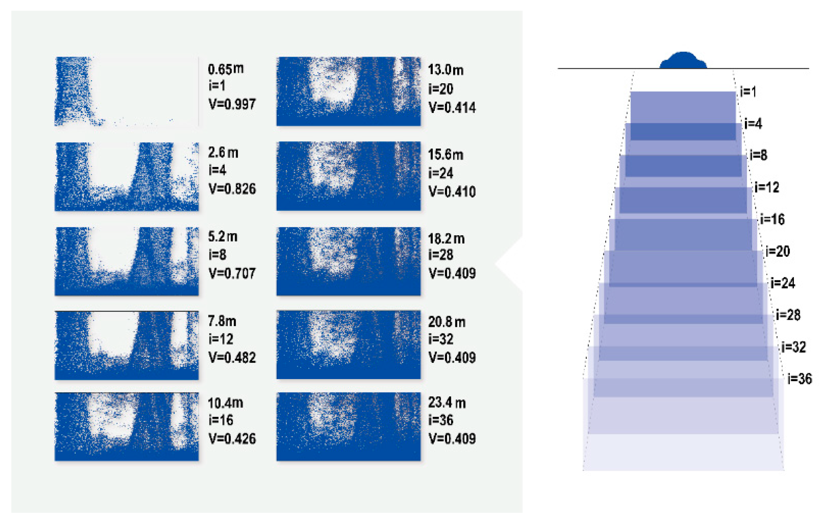
2.3.2. Calculation of the Visibility Index

From an animal perspective, visibility is ecologically significant when it reflects the area exposed to predator or prey. Guided by target detection, we developed the visibility calculation process. The complex shapes and fine details of natural objects pose a huge challenge to our computational process. Therefore, we simplified the target contour and replaced it with the minimum enclosing rectangle of the target (Figure 2e–g). According to the morphological characteristics of a tiger, shoulder height (h) and body length (w) formed the minimum enclosing rectangle (d_θ,i) (θ: angle between the minimum enclosing rectangle and the boar’s nest; i: the distance between the minimum enclosing rectangle and the boar’s nest) (Figure 2f). Visibility was expressed as the exposed area of the target object (Figure 2f). The obscured area formed by the point cloud (p_θ,i) surrounded by a cuboid (D_θ,i × w × h) projection onto the minimum enclosing rectangle (parallel to the ground and along the θ direction) (Figure 2e). The exposed area (N − n_θ,i) was related to the area (n_θ,i) obscured by the projection of the point cloud to the minimum enclosing rectangle (Figure 2f). We calculated the visibility of each minimum enclosing rectangle and generated a visibility picture for wider application. Although the pattern on the surface of the tiger was presumed to be conducive to hiding, it was not included in our analysis because we could not objectively quantify how disturbing the pattern was to the wild boar. The exact description of the point cloud projected to the minimum enclosing rectangle is given in the following formula (Table S10):

$${\mathrm{V}}_{\mathsf{\theta },\mathrm{i}}=\frac{\mathrm{N}-{\mathrm{n}}_{\mathsf{\theta },\mathrm{i}}}{\mathrm{N}}\times 100\%$$

(1)

$$\mathrm{N}=\mathrm{w}\times \mathrm{h}$$

(2)

V_θ,i is the visibility of d_θ,i.; N is the area of the minimum enclosing rectangle; and n_{θ, i} is the area where the minimum enclosing rectangle was obscured by the point cloud.

The range of point clouds projected to the minimum enclosing rectangle (Table S10):

$${\mathrm{p}}_{\mathsf{\theta },\mathrm{i}}=\{\begin{array}{c}\mathrm{y}1<\mathrm{y}<\mathrm{y}2\\ \mathrm{x}1<\mathrm{x}<\mathrm{x}2\\ 0<\mathrm{z}<\mathrm{h}\end{array}$$

(3)

where x, y, z represents the coordinates of the point cloud projected to the minimum enclosing rectangle.

x1 represents the nearest boundary of the point cloud.

x2 represents the farthest boundary of the point cloud.

y1 and y2 represent the leftmost and rightmost boundaries of the point cloud.

2.3.3. Simulated Scene Showing the Tiger Near the Nest

The occurrence of interspecific interaction is a dynamic process, so calculating the visibility of a single position cannot reflect the change of visibility when interspecific interaction occurs. A complete record of the tiger’s approach to the nest would be almost impossible in the wild. Therefore, we simulated the change in visibility as the tiger approached the boar by calculating the visibility at any location and then sampling the visibility by distance. In the sample range, we set the equivalent rectangle (d_θ,i) at different distances (D_θ,i) in all directions (θ = 1–360°) (Figure 2e). In the same direction, we graded (i) the distance with the interval determined by the step length of the tiger.

2.4. Statistical Analysis

To test whether the ambush behavior of the tigers affected visibility, we performed two visibility scenes—one at 1 m (h) and one at 0.5 m (h). After obtaining the visibility, we divided the visibility into a total of 10 gradients from 0 to 9, and extracted the distance (D) within each visibility gradient in different scene groups (1 m and 0.5 m). We used the Kruskal–Wallis to test whether there was a difference in distance between scene groups with the same visibility gradient [38]. If there was a difference, it indicated that tigers can affect visibility by ambush.

To visualize the changing process of visibility, we extracted the visibility and distance indicators in all directions (θ) and explored the changing pattern of visibility with distance. We assumed that the variation pattern of visibility with distance was nonlinear, so we tested the fitting effect with R² and p-value. We also calculate the derivative of the curve to evaluate the rate of change in visibility. Kruskal–Wallis test and nonlinear fitting were based on IBM SPSS statistics 26 (IBM, Armonk, NY, USA). Derivative calculations were based on R 3.6.3 (R Core Team).

3. Results

3.1. Visibility Calculation

We used the perpendicular to the ground minimum enclosing rectangle to represent a predator, and then we verified that the shielding effects of forest structure components on this minimum enclosing rectangle have a cumulative effect with the change of distance in the horizontal direction (Figure 3). As the distance from the boar’s nest decreased from 23.4 m to 0.65 m, the visibility increased from 0.409 to 0.997. The minimum enclosing rectangles with visibility information turn visibility changes into a continuous and observable process (Figure 3).

We hypothesized that the Amur tigers could hunt the wild boar from any direction around the nest; we simulated the process of tigers appearing around the nests in 360° directions (θ = 1–360°), and the exposed area within the minimum enclosing rectangle in any direction represented the tiger visibility. The minimum enclosing rectangle was 2.1 m wide (average body length of the Amur tiger, w), and 1 m/0.5 m high (average shoulder height of the Amur tiger while standing and in ambush behavior, respectively, h) [39], while the distance between the minimum enclosing rectangle in the same direction was 0.65 m (average step length of Amur tigers) [40]. Thus, for any nests, we obtained 14,040 minimum enclosing rectangles (i = 39 for each direction) for each height of 1 m and 0.5 m, corresponding to each behavior (Figure 4, Tables S5 and S6).

We took each sample as an object and fitted the pattern of visibility change with the distance to the nest in two scenarios (h = 1 m and 0.5 m) to explore the general pattern of visibility change in 3D forest (Figure 4, Tables S7 and S8). The results indicated that the relationship between the change in visibility and distance conformed to logarithmic functions (p < 0.01, R² > 0.7) for all objects (Figure 4, Tables S7 and S8). Visibility had a cumulative effect; it rapidly declined at the initial stage, was stable at a relatively low level, and it gradually approached the lowest value. The derivative of the curves also showed that the visibility changed rapidly over a range of 0–5 m for 40 samples, after which the rate of change flattened out.

3.2. 3D Forest Structure Mediated Predation Strategy

Our results verify that the ambush behavior of tigers does affect visibility (Figure 5, Table S9). Ambush behavior makes the tiger move closer to the nest than standing behavior (Figure 5, Table S9). Within the same visibility gradient, the distance from the nest to the ambush behavior was significantly shorter than that to the standing behavior (Figure 5, Table S9). The Amur tiger is an opportunist stalk-and-ambush solitary hunter, relying on a combination of 3D forest structure and stalking behavior to enhance the concealment ability to overcome their prey. Thus, our result also indicated that, before exposing itself to the wild boar, the Amur tiger adopts the optimal concealment strategy as a predation strategy.

3.3. 3D Forest Structure and Predation Mediated Anti-Predation Strategy

Our findings indicate that wild boars bite off the shrubs around their nests to expose themselves as a possible game strategy of predation and anti-predation between the tiger and wild boar (Figure 5, Table S9). Although the ambush behavior allows the tiger to approach the wild boar, we found that within 0–5 m of the nest, ambush behavior had lost its advantage in making the tiger move closer to the wild boar since the visibility maintained the tiger at a high level, exposing the tiger and wild boar to each other (Figure 4 and Figure 5). Modifications to the 3D forest structure may provide a safer environment for wild boar to avoid predation through early detection. Early detection could allow the wild boar to employ appropriate anti-predation strategies that increase their probability of survival [41]. Wild boars used a passive anti-predation approach to enhance concealment within >5 m of the nest; however, within 0–5 m of the nest, exposure and early detection as an active anti-predation strategy could lower the risk of predation.

4. Discussion

We discovered that the pattern of visibility change with distance in wildlife was accumulated by the 3D forest structure and conformed to the logarithmic function (Figure 4, Tables S7 and S8). For the first time, we quantified wildlife visibility in the 3D environment as the exposed area of the minimum enclosing rectangle at any angle and distance, which is a useful process-oriented method that reflects predation and anti-predation. A realistic application scenario of our paradigm is to quantify changes in visibility along a complex moving trajectory (the trajectory has multiple inflection points) (Figure 6). When we apply our paradigm to similar problems, we first need to capture the complex animal movement trajectory. Second, we register the trajectory and the environmental point cloud to the same coordinate system (Figure 6a; simulated animal trajectories in environment point clouds). Third, we use our workflow to generate visibility at any angle and distance within the sample. Fourth, we extract the coordinates of points of interest on the trajectory and use the extracted coordinates to screen the visibility index. Finally, we obtain the change in visibility along the trajectory (Figure 6b; on the trajectory, 100 interest points are extracted along the moving direction to form the change of visibility; we also preliminarily explore the relationship between the distance from the target and the change of visibility). When our paradigm is combined with graphic processing, feature recognition can be performed on the point cloud image in the minimum enclosing rectangle.

One of the important findings from this study was that Amur tigers take advantage of forest features on a fine scale and adopt an ambush behavior to significantly reduce their visibility (Figure 5). Before this study, researchers assumed that ambush was related to visibility, but none had quantified the relationship between ambush and visibility [22,42]. Passive remote sensing techniques have been used to analyze visibility in open landscapes [42]. However, due to canopy occlusion in a forest ecosystem, remote sensing images cannot obtain the data under the canopy to carry out visibility analysis. Quantifying changes in visibility at a fine scale from BLS data, we created an opportunity to test the ambush-habitat hypothesis [42] in a forest ecosystem. Amur tigers crawl to conceal themselves in forest habitats and minimize their visibility and ambush prey species at the nearest distance to enhance prey ‘catchability’. We objectively established that ambush behaviors can diminish visibility through simulation. Our method could be used to investigate the ambush-habitat hypothesis in forests. Therefore, our research framework can help understand how to simulate ambush predator habitat, how precise details of a specific habitat affect predator–prey interactions, and also how environmental factors mediate wildlife coexistence in a forest ecosystem.

The other important finding of our study is that wild boar, an excellent structural modifier [24,33], constructs nests not only to enhance fitness, but also as an anti-predation strategy in the forest ecosystem. Wild boars only bite off the shrubs within about a 5 m-radius around their nests. Consequently, wild boar visibility is maintained at a high level in this area, but beyond 5 m, it is maintained at a low level (Figure 4). In the ‘visibility fortress’—within 5 m radius around the nest—wild boars are relatively safe because the ambush behavior of the tiger is defeated; an emergent response of wild boar will reduce the ‘catchability’ (Figure 4 and Figure 7). Combined with field investigations and tiger ambush behavior [43], it is reasonable to speculate that the ‘visibility fortress’ is an anti-predation strategy similar to the one of ‘early detection’ [22,41]. Habitats with good cover and camouflage are not conducive to the detection of concealing predators; therefore, prey species have to expose themselves and increase the visibility of the predator by choosing more open areas [22,44]. At a fine-scale forest ecosystem, it might often be necessary to study the behavior of predators [45] before the environmental factor-mediated behavioral response of prey species; for example, in our study, the ‘visibility fortress’ is the response of wild boars to the ambush behavior of tigers and the landscape heterogeneity.

Amur tiger–wild boar interactions or the predation/anti-predation behavior in this study can indeed be evolutionary ‘arm races’, with the specific form of coevolutionary traits depending on forest structure. In this study, elements of both tigers’ and wild boars’ strategies correspond to each other. Their main purposes are to take advantage of landscape heterogeneity. Game strategies of predation and anti-predation in the forest made tigers evolve into ambush hunters to get closer to wild boars; in response, wild boars developed a ‘visibility fortress’ to detect tigers in advance. There is a little tradeoff between concealment and exposure [20,22,24,44]. Our results about predation and anti-predation between tigers and wild boars provide new empirical evidence for this game strategy.

5. Conclusions

In conclusion, our research framework (Figure 2) provides a new perspective for exploring the role of vision in the process of interspecific relationships on a fine scale. Our research framework revealed novel results. Through the reconstruction of the spatial structure of the forest and simulating the appearance of tigers around the wild boars, the visibility index was used to explore ambush hunting. Tigers and boars use the environment to change their visibility to their own advantage. Our framework may provide guidance for exploring the process of interspecific relationships in three-dimensional space.

References

1. Letten, A.D.; Stouffer, D.B. The mechanistic basis for higher-order interactions and non-additivity in competitive communities. Ecol. Lett. 2019, 22, 423–436. [Google Scholar] [CrossRef] [PubMed]
2. Gallien, L.; Zimmermann, N.E.; Levine, J.M.; Adler, P.B. The effects of intransitive competition on coexistence. Ecol. Lett. 2017, 20, 791–800. [Google Scholar] [CrossRef]
3. Terborgh, J.W. Toward a trophic theory of species diversity. Proc. Natl. Acad. Sci. USA 2015, 112, 11415. [Google Scholar] [CrossRef] [PubMed] [Green Version]
4. Chase, J.M.; Abrams, P.A.; Grover, J.P.; Diehl, S.; Chesson, P.; Holt, R.D.; Richards, S.A.; Nisbet, R.M.; Case, T.J. The interaction between predation and competition: A review and synthesis. Ecol. Lett. 2002, 5, 302–315. [Google Scholar] [CrossRef]
5. Chesson, P.; Kuang, J.J. The interaction between predation and competition. Nature 2008, 456, 235–238. [Google Scholar] [CrossRef] [PubMed]
6. Vázquez, D.P.; Lomáscolo, S.B.; Maldonado, M.B.; Chacoff, N.P.; Dorado, J.; Stevani, E.L.; Vitale, N.L. The strength of plant–pollinator interactions. Ecology 2012, 93, 719–725. [Google Scholar] [CrossRef] [PubMed] [Green Version]
7. Zhang, Q.; Buckling, A. Antagonistic coevolution limits population persistence of a virus in a thermally deteriorating environment. Ecol. Lett. 2011, 14, 282–288. [Google Scholar] [CrossRef]
8. Allesina, S.; Levine, J.M. A competitive network theory of species diversity. Proc. Natl. Acad. Sci. USA 2011, 108, 5638. [Google Scholar] [CrossRef] [PubMed] [Green Version]
9. Bairey, E.; Kelsic, E.D.; Kishony, R. High-order species interactions shape ecosystem diversity. Nat. Commun. 2016, 7, 12285. [Google Scholar] [CrossRef]
10. Bastolla, U.; Fortuna, M.A.; Pascual-Garcia, A.; Ferrera, A.; Luque, B.; Bascompte, J. The architecture of mutualistic networks minimizes competition and increases biodiversity. Nature 2009, 458, 1018–1020. [Google Scholar] [CrossRef]
11. Pringle, R.M.; Kartzinel, T.R.; Palmer, T.M.; Thurman, T.J.; Fox-Dobbs, K.; Xu, C.C.Y.; Hutchinson, M.C.; Coverdale, T.C.; Daskin, J.H.; Evangelista, D.A.; et al. Predator-induced collapse of niche structure and species coexistence. Nature 2019, 570, 58–64. [Google Scholar] [CrossRef]
12. Stachowicz, J.J.; Fried, H.; Osman, R.W.; Whitlatch, R.B. Biodiversity, invasion resistance, and marine ecosystem function: Reconciling pattern and process. Ecology 2002, 83, 2575–2590. [Google Scholar] [CrossRef]
13. Zhang, H.; Bearup, D.; Nijs, I.; Wang, S.; Barabás, G.; Tao, Y.; Liao, J. Dispersal network heterogeneity promotes species coexistence in hierarchical competitive communities. Ecol. Lett. 2021, 24, 50–59. [Google Scholar] [CrossRef]
14. Eklöv, P.; VanKooten, T. Faciliation among piscivorous predators: Effects of prey habitat use. Ecology 2001, 82, 2486–2494. [Google Scholar] [CrossRef] [Green Version]
15. Dröge, E.; Creel, S.; Becker, M.S.; M’soka, J. Risky times and risky places interact to affect prey behaviour. Nat. Ecol. Evol. 2017, 1, 1123–1128. [Google Scholar] [CrossRef]
16. Stier Adrian, C.; Samhouri Jameal, F.; Novak, M.; Marshall Kristin, N.; Ward Eric, J.; Holt Robert, D.; Levin Phillip, S. Ecosystem context and historical contingency in apex predator recoveries. Sci. Adv. 2016, 2, e1501769. [Google Scholar] [CrossRef] [Green Version]
17. Smith, J.G.; Tomoleoni, J.; Staedler, M.; Lyon, S.; Fujii, J.; Tinker, M.T. Behavioral responses across a mosaic of ecosystem states restructure a sea otter–urchin trophic cascade. Proc. Natl. Acad. Sci. USA 2021, 118, e2012493118. [Google Scholar] [CrossRef] [PubMed]
18. Molnár, P.K.; Bitz, C.M.; Holland, M.M.; Kay, J.E.; Penk, S.R.; Amstrup, S.C. Fasting season length sets temporal limits for global polar bear persistence. Nat. Clim. Chang. 2020, 10, 732–738. [Google Scholar] [CrossRef]
19. Creel, S.; Winnie, J.; Maxwell, B.; Hamlin, K.; Creel, M. Elk alter habitat selection as an antipredator response to wolves. Ecology 2005, 86, 3387–3397. [Google Scholar] [CrossRef]
20. Loarie, S.R.; Tambling, C.J.; Asner, G.P. Lion hunting behaviour and vegetation structure in an African savanna. Anim. Behav. 2013, 85, 899–906. [Google Scholar] [CrossRef] [Green Version]
21. Swanson, A.; Caro, T.; Davies-Mostert, H.; Mills, M.G.L.; Macdonald, D.W.; Borner, M.; Masenga, E.; Packer, C. Cheetahs and wild dogs show contrasting patterns of suppression by lions. J. Anim. Ecol. 2014, 83, 1418–1427. [Google Scholar] [CrossRef]
22. Davies, A.B.; Tambling, C.J.; Marneweck, D.G.; Ranc, N.; Druce, D.J.; Cromsigt, J.P.G.M.; le Roux, E.; Asner, G.P. Spatial heterogeneity facilitates carnivore coexistence. Ecology 2021, 102, e03319. [Google Scholar] [CrossRef] [PubMed]
23. Schmitz, O.J. Predators avoiding predation. Proc. Natl. Acad. Sci. USA 2008, 105, 14749. [Google Scholar] [CrossRef] [PubMed] [Green Version]
24. Manicom, C.; Schwarzkopf, L.; Alford, R.A.; Schoener, T.W. Self-made shelters protect spiders from predation. Proc. Natl. Acad. Sci. USA 2008, 105, 14903. [Google Scholar] [CrossRef] [Green Version]
25. Olsoy, P.J.; Forbey, J.S.; Rachlow, J.L.; Nobler, J.D.; Glenn, N.F.; Shipley, L.A. Fearscapes: Mapping Functional Properties of Cover for Prey with Terrestrial LiDAR. BioScience 2015, 65, 74–80. [Google Scholar] [CrossRef] [Green Version]
26. Muto, A.; Lal, P.; Ailani, D.; Abe, G.; Itoh, M.; Kawakami, K. Activation of the hypothalamic feeding centre upon visual prey detection. Nat. Commun. 2017, 8, 15029. [Google Scholar] [CrossRef] [PubMed] [Green Version]
27. Mugan, U.; MacIver, M.A. Spatial planning with long visual range benefits escape from visual predators in complex naturalistic environments. Nat. Commun. 2020, 11, 3057. [Google Scholar] [CrossRef]
28. Aben, J.; Signer, J.; Heiskanen, J.; Pellikka, P.; Travis, J.M.J. What you see is where you go: Visibility influences movement decisions of a forest bird navigating a three-dimensional-structured matrix. Biol. Lett. 2021, 17, 20200478. [Google Scholar] [CrossRef] [PubMed]
29. Vierling, K.; Vierling, L.; Gould, W.; Martinuzzi, S.; Clawges, R. LiDAR: Shedding new light on habitat characterization and modeling. Front. Ecol. Environ. 2008, 6, 90–98. [Google Scholar] [CrossRef] [Green Version]
30. Davies, A.B.; Asner, G.P. Advances in animal ecology from 3D-LiDAR ecosystem mapping. Trends Ecol. Evol. 2014, 29, 681–691. [Google Scholar] [CrossRef]
31. Yang, H.; Dou, H.; Baniya, R.K.; Han, S.; Guan, Y.; Xie, B.; Zhao, G.; Wang, T.; Mou, P.; Feng, L.; et al. Seasonal food habits and prey selection of Amur tigers and Amur leopards in Northeast China. Sci. Rep. 2018, 8, 6930. [Google Scholar] [CrossRef] [PubMed]
32. Hailong, D.; Haitao, Y.; James, L.D.S.; Limin, F.; Tianming, W.; Jianping, G. Prey selection of Amur tigers in relation to the spatiotemporal overlap with prey across the Sino–Russian border. Wildl. Biol. 2019, 2019, 1–11. [Google Scholar]
33. Luskin, M.S.; Brashares, J.S.; Ickes, K.; Sun, I.F.; Fletcher, C.; Wright, S.J.; Potts, M.D. Cross-boundary subsidy cascades from oil palm degrade distant tropical forests. Nat. Commun. 2017, 8, 2231. [Google Scholar] [CrossRef] [PubMed] [Green Version]
34. Fernández-Llario, P. Environmental correlates of nest site selection by wild boar Sus scrofa. Acta Theriol. 2004, 49, 383–392. [Google Scholar] [CrossRef]
35. Hayward, M.W.; Jędrzejewski, W.; Jêdrzejewska, B. Prey preferences of the tiger Panthera tigris. J. Zool. 2012, 286, 221–231. [Google Scholar] [CrossRef]
36. Van der Zande, D.; Hoet, W.; Jonckheere, I.; van Aardt, J.; Coppin, P. Influence of measurement set-up of ground-based LiDAR for derivation of tree structure. Agric. For. Meteorol. 2006, 141, 147–160. [Google Scholar] [CrossRef]
37. Henning, J.; Radtke, P. Ground-based Laser Imaging for Assessing Three-dimensional Forest Canopy Structure. Photogramm. Eng. Remote Sens. 2006, 72, 1349–1358. [Google Scholar] [CrossRef]
38. Li, C.; Gan, Y.; Zhang, C.; He, H.; Fang, J.; Wang, L.; Wang, Y.; Liu, J. “Microplastic communities” in different environments: Differences, links, and role of diversity index in source analysis. Water Res. 2021, 188, 116574. [Google Scholar] [CrossRef] [PubMed]
39. Yudakov, A.G.; Nikolaev, I.G. Winter ecology of the Amur tiger: Based upon observations in the west-central Sikhote-Alin Mountains 1970–1973, 1996–2010. J. Wildl. Manag. 2014, 1–2. [Google Scholar] [CrossRef]
40. Pikunov; Mitchell; Dunishe; Li, B. A Guide to Wildlife Tracks in the Far East; Northeast Forestry University Press: Harbin, China, 2008. [Google Scholar]
41. Samia, D.S.M.; Nomura, F.; Blumstein, D.T. Do animals generally flush early and avoid the rush? A meta-analysis. Biol. Lett. 2013, 9, 20130016. [Google Scholar] [CrossRef] [PubMed] [Green Version]
42. Hopcraft, J.G.C.; Sinclair, A.R.E.; Packer, C. Planning for success: Serengeti lions seek prey accessibility rather than abundance. J. Anim. Ecol. 2005, 74, 559–566. [Google Scholar] [CrossRef]
43. Yudakov, A.G.; Nikolaev, I.G. Winter Ecology of the Amur Tiger; Dalnauka: Vladivostok, Russia, 2012. [Google Scholar]
44. Iason, G.R.; Prins, H.H.T. Dangerous Lions and Nonchalant Buffalo. Behaviour 1989, 108, 262–296. [Google Scholar] [CrossRef]
45. Lima, S.L. Putting predators back into behavioral predator–prey interactions. Trends Ecol. Evol. 2002, 17, 70–75. [Google Scholar] [CrossRef]
Figure 1. Study system and experimental design. (a) Study area. The type of land cover in the study area consisted mainly of Taiga Forest. The 241 gray triangles represent the locations of boar nests obtained during our field survey, and the 20 red circles represent the locations of boar nests used to collect point cloud data in this study. (b,c) Sample internal point cloud data display. Point cloud data from the sample of 2021-05-19-09-47-40. (b) Top view of point cloud data. (c) Flat view of point cloud data. (d) The purpose of our study was to find a more general rule, which required that the environmental conditions of 20 samples were different. We used three indicators—canopy height, diameter at breast height, and canopy cover—to represent the environmental conditions. The Kruskal–Wallis test shows that the environmental conditions of the 20 quadrats were significantly different (p < 0.001 ***). The data are z-scaled to be presented in the same dimension.
Remotesensing 14 03730 g001
Figure 2. Workflow of the research framework. (a) Initial field survey to obtain the location of wild boar nests. (b) Point cloud data collection. The red cube is an artificial fence that represents the location of the wild boar’s nest to accurately identify it when processing the point cloud data. The red line is the trajectory when the point cloud data are collected by backpack laser scanning (BLS).This trajectory can improve the consistency of point cloud data with real things. (c,d) LiDAR 360 was used to preprocess point cloud data. (c) Original point cloud data. The range is larger than the sample range, and the lowest point cloud is not on the same horizontal plane. (d) Pre-processed point cloud data. The sample range is a circular area with the wild boar’s nest as the center and a radius of 25 m. The lowest point cloud is in the same horizontal plane. (e,f) Calculation of the visibility using the minimum enclosing rectangle (e), and positioning of the minimum enclosing rectangle to simulate the tiger near the nest (f), using GvEcology. We set up a minimum enclosing rectangle in 1–360 directions (θ) around the nest and 39 distance gradients (i) in each direction (θ) (f). (g) Use of (ef) with point cloud data and mapping of an actual scene.
Remotesensing 14 03730 g002
Figure 3. A sample of the minimum enclosing rectangle used to calculate visibility. Data were obtained from sample 2021-05-18-12-01-28, θ = 4. The blue portion of each minimum enclosing rectangle indicates the area (nθ,i) obscured by the projection of the point cloud. The white portion indicates the exposed area, which indicates visibility.
Remotesensing 14 03730 g003
Figure 4. Pattern of visibility change with distance. Within each sample, the change pattern between distance and visibility conforms to a logarithmic curve (Visibility= a – b × log (Distance), p < 0.05, R2 > 0.7). The gray line perpendicular to the X axis is 5 m.
Remotesensing 14 03730 g004
Figure 5. Ambush behaviors can be closer to the wild boar than the standing behaviors. Blue represents the standing behaviors; red represents the ambush behaviors. Gray shade indicates that the two groups of data are not significantly different (p > 0.05). The red line is 5 m, the blue line is 10 m. Within 5 m, ambush behaviors no longer brought tigers closer to the nest.
Remotesensing 14 03730 g005
Figure 6. Changes in visibility along the simulated animal trajectories. Point cloud data from the sample of 2021-05-19-09-47-40. (a) Simulated animal trajectories in environment point clouds. (b) The relationship (R = −0.646, p < 0.01 **) between the distance from the target and the change of visibility.
Remotesensing 14 03730 g006
Figure 7. ‘Visibility fortress’ hint. Visibility data from sample 2021-05-17-11-08-33. The center of the ‘visibility fortress’ is the location of the boar’s nest. The original visibility ranges from 0 to 1. To clearly show the spatial distribution of the visibility on a 50-m scale, we scaled the visibility to 0–10. We used a triangular irregular network surface to display the visibility surface to completely preserve the distribution details of the visibility in the 3D space. We did not use the model to fit the visibility surface because we were not sure if those details were important in the 3D space.
Remotesensing 14 03730 g007
Publisher’s Note: MDPI stays neutral with regard to jurisdictional claims in published maps and institutional affiliations.