Shuffle-CDNet: A Lightweight Network for Change Detection of Bitemporal Remote-Sensing Images

Abstract

Change detection is an important task in remote-sensing image analysis. With the widespread development of deep learning in change detection, most of the current methods improve detection performance by making the network deeper and wider, but ignore the inference time and computational costs of the network. Therefore, this paper proposes a lightweight change-detection network called Shuffle-CDNet. It accepts the six-channel image that concatenates the bitemporal images by channel as the input, and it adopts the backbone network with channel shuffle operation and depthwise separable convolution layers. The classifier uses a lightweight atrous spatial pyramid pooling (Light-ASPP) module to reduce computational costs. The edge-information feature extracted by a lightweight branch is integrated with the shallow and deep features extracted by the backbone network, and the spatial and channel attention mechanisms are introduced to enhance the expression of features. At the same time, logit knowledge distillation and data augmentation techniques are used in the training phase to improve detection performance. Experimental results showed that the proposed method achieves a better balance in computational efficiency and detection performance compared with other advanced methods.

1. Introduction

With the continuous increase in the world’s population and the accelerated urbanization process, the global surface has also undergone significant changes, and the study of the interaction between urbanization and environmental change has received more attention. Given that the change detection based on remote-sensing images has come into being, change detection is one of the important research directions of remote-sensing technology, which uses registered remote-sensing images of the same area at different times to obtain change information. It assigns binary classification labels (changed or unchanged) to each pixel of images. Change detection of remote-sensing images is widely used in many fields such as monitoring urban change and development, assessing earthquake and flood disasters, and monitoring crop growth status.

In the early stage of the development of change-detection technology, traditional methods are generally adopted. It can be divided into two steps. First, the difference map is generated by appropriate methods. For example, the difference map is obtained by using arithmetic operations of difference calculation and ratio calculation. Kasischke et al. [1] proposed change vector analysis (CVA). Change vectors are calculated by subtracting pixel vectors of bitemporal images. Principal component analysis (PCA) is applied to bitemporal images separately and the difference map is generated by comparing the results [2]. Second, the binary change map is obtained by using the threshold method, clustering method (such as K-means clustering [3] and fuzzy C-means clustering [4]) or using support vector machines [5], Markov random field models [6], etc. For example, the change map is achieved by partitioning the feature vector space into two clusters using K-means clustering with k = 2 and then assigning each pixel to one of the two clusters [3]. Nemmour et al. [5] utilized binary SVM to obtain change information, which considered the changed pixels as positive and considered the unchanged pixels as negative. These traditional methods are generally designed with the help of manual feature selection and extraction, which are susceptible to noise interference and often perform poorly in the complex scenarios, especially on high-spatial-resolution remote-sensing images.

Recently, deep-learning technology, especially convolutional neural networks (CNN), has achieved excellent performance and has been extensively applied in remote sensing with its computing power to change detection tasks. Many deep-learning-based change-detection methods have demonstrated better performances than traditional methods. Some attempts use CNN to extract change information based on siamese network structure. For example, Zhang et al. [7] utilized the siamese CNN to extract the spectral-spatial joint representation. Then, the change map was generated through feature fusion and discrimination learning. Daudt et al. [8] proposed two siamese architectures, FC-Siam-conc and FC-Siam-diff, for change detection. The former concatenated the two skip connections during the decoding steps and the latter concatenated the absolute value of their difference. Zhang et al. [9] proposed a deeply supervised image fusion network (IFN). The extracted deep features by a two-stream siamese backbone network were fed into a deeply supervised difference discrimination network. Other methods use CNN based on the early converged network by concatenating the two images before passing them through the network. Nakamura et al. [10] proposed a U-net-based network to detect the new construction of buildings in developing areas based on the early converged network. The skip connections help generate good results without losing information. Zheng et al. [11] proposed an early converged network based on an encoding–decoding structure named CLNet, which incorporated multiscale features and multilevel contextual information by embedding cross-layer blocks (CLBs) in the encoder. Peng et al. [12] proposed an early converged network based on UNet++. It utilized both global and fine-grained information to generate feature maps. Then, the fusion strategy of multiple side outputs was adopted to combine change maps from different semantic levels.

With the continuous improvement of the spectral and spatial resolution of remote-sensing images, recurrent neural networks (RNN) and self-attention mechanisms have been widely used in the process of change detection to capture long-range contextual information. Wang et al. [13] proposed the SiamCRNN to fuse time-space-spectral information. However, the input of SiamCRNN is small neighborhood blocks, which are difficult to use to obtain global relevant information. To solve this problem, Chen et al. [14] proposed the STANet network, which inputs the global features extracted by the ResNet18 network into the self-attention mechanism module, and captures the long-range spatial-temporal dependencies for learning better representations. Some methods also introduce spatial attention or channel attention mechanisms to improve feature expression [9,15,16,17]. For example, Song et al. [15] proposed AGCDetNet, which added the learned spatial attention to the deep features to promote discrimination between the changed objects and the background. It utilized the channel-wise attention-guided interference filtering unit to enhance the representation of multilevel features, and the transformer had powerful and robust performance in various computer vision tasks after being proposed. Chen et al. [18] proposed Bit-CD, which expressed the bitemporal image to a few tokens and used a transformer encoder to model contexts in the compact token-based space-time. The tokens were fed back to the pixel space for refining the original features via a transformer decoder. Other transformer-based and swin-transformer-based methods also show good performance in change detection tasks [19,20,21]. For example, Zhang et al. [21] proposed SwinSUNet, which contains an encoder, fusion, and decoder, and all of them use swin transformer blocks as basic units. However, these methods are not dominant in terms of computation efficiency.

It can be seen that to enhance the expression ability of features, some attempts have been made to solve the problem by using deeper or wider networks, and the integration of more attention mechanism modules or transformer-based structures. However, these strategies also increase computational costs and are extremely unfriendly to the inference time. At present, many works have begun to pay attention to the design of lightweight networks, such as directly manual design [22,23,24,25,26], including the ShuffleNet series [27,28]. For example, Howard et al. [24] utilized depthwise separable convolutions to build MobileNets, which factorize a standard convolution into a depthwise convolution and a 1 × 1 convolution called a pointwise convolution. Meanwhile, knowledge distillation [29,30,31] can also reduce the computational costs of models. Knowledge distillation is a procedure for model compression, in which a small (student) model is trained to match a large pre-trained (teacher) model. Knowledge is transferred from the teacher model to the student by minimizing a loss function, aimed at matching softened teacher logits as well as ground-truth labels [29]. Although various studies have focused on increasing the accuracy in change detection tasks, few studies focus on increasing the computational efficiency. Chen et al. [32] proposed a lightweight multiscale spatial pooling network to detect changes in SAR images. Multiscale pooling kernels were equipped in a convolutional network to exploit the spatial information. Wang et al. [33] proposed a lightweight network that replaces the regular convolutional layers with bottlenecks and employs convolutional kernels with some non-zero entries, but it does not give specific network parameters and operation metrics, making it difficult to evaluate the efficiency of the network. Song et al. [34] proposed 3M-CDNet and its lightweight network 1M-CDNet used for change detection tasks. Deformable convolution is integrated into the residual network and shallow and deep features are fused. 1M-CDNet is simpler than the 3M-CDNet in the classifier, but the application of deformable convolution cannot further reduce the inference time. In these lightweight networks, the down-/upsampling is used to increase the receptive field, resulting in spatial-detail information loss and perhaps a failure to precisely depict boundaries. To solve this problem, some methods attempt to integrate edge information or combine edge detection with contextual aggregation. For example, Guo et al. [35] proposed an edge-preservation network named SG-EPUNet, which designs the edge-detection branch based on residual networks and fuses with contextual information to refine fuzzy boundaries. Liu et al. [36] utilized the edge-constraint loss to constrain the differences between the boundaries of the predicted mask and the ground truth, which were extracted by the Sobel filters. Yang et al. [37] composed the backbone network and edge-perception network and utilized an edge-aware loss to obtain accurate results. Inspired by this spirit, this paper designs a lightweight network named Shuffle-CDNet for the change-detection task and a lightweight edge-information feature-enhancement branch is involved. Shuffle-CDNet better balances computing costs, inference time and detection performance compared with 1M-CDNet and other methods.

The main contributions of this paper are summarized as follows. A lightweight network named Shuffle-CDNet is proposed, which uses a lightweight backbone network and a concise classifier. The backbone consists of the building blocks of ShuffleNet v2 [28], which adopts channel shuffle, depthwise separable convolutions, and other operations to reduce computational costs. The classifier uses the Light-ASPP module to classify the features extracted by the backbone and generate a binary change map. To improve the edge detection in the changed regions, especially for small objects, the lightweight edge-information feature-enhancement branch of the changed regions is designed and integrated with the shallow and deep features of the backbone network, and to enhance the feature-expression ability, the spatial and channel attention mechanism are introduced in the backbone. At the same time, the logit knowledge-distillation technology is used to distill the student network Shuffle-CDNet with 3M-CDNet [34] as the teacher network. 3M-CDNet can provide supervision information and improve the detection performance of Shuffle-CDNet. In addition, the online data-augmentation strategy is used in the training phase, and the Tversky loss function is introduced to balance the accuracy and recall of the detection. Without sacrificing the detection performance of the network, the computational costs and inference time of Shuffle-CDNet are better than most other advanced networks. The balance between the detection performance and the computational costs is well-realized.

2. Proposed Methods

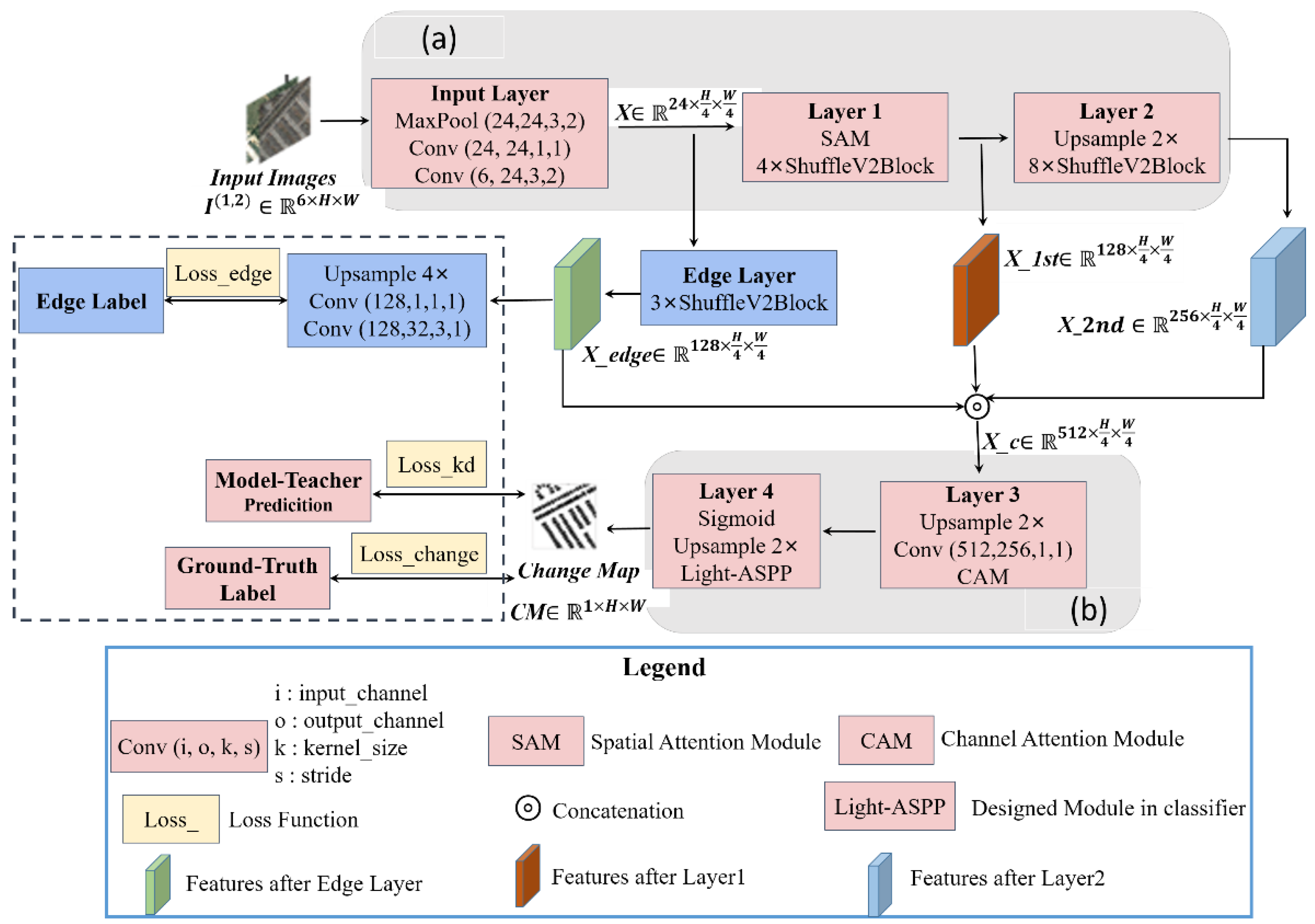
The proposed network named Shuffle-CDNet mainly consists of the backbone and the classifier. A lightweight edge-information feature-enhancement branch is also involved. The workflow of the Shuffle-CDNet with a flexible modular design is shown in Figure 1.

The input of Shuffle-CDNet is a six-channel image $I^{\left(1,2\right)}\in {ℝ}^{6\times H\times W}$ obtained by contacting the bitemporal images in the channel dimension. It passes through the Input Layer, Layer 1 and Layer 2 to obtain the low-dimensional features $X\in {ℝ}^{24\times \frac{H}{4}\times \frac{W}{4}}$, $X\_1st\in {ℝ}^{128\times \frac{H}{4}\times \frac{W}{4}}$, and $X\_2nd\in {ℝ}^{256\times \frac{H}{4}\times \frac{W}{4}}$, respectively. A lightweight edge-information feature-enhancement branch of the changed regions is designed; that is, shallow feature $X$ passes through the Edge Layer module to obtain edge-information feature $X\_edge\in {ℝ}^{128\times \frac{H}{4}\times \frac{W}{4}}$. The $X\_1st$, $X\_2nd,$ and $X\_edge$ are contacted in the channel dimension and output through Layer 3 and Layer 4. The extracted pixel features are classified into two categories: changed and unchanged. Layer 3 consists of a channel attention module (CAM), a 1 × 1 convolution layer, and a upsample layer. The upsample layers involved in the network are implemented by bilinear interpolation. Layer 4 consists of a Light ASPP module, an upsample layer, and a sigmoid layer. Finally, a binary change map $CM\in {ℝ}^{1\times H\times W}$ is output by a fixed threshold segmentation. It is worth noting that the part inside the dashed box in Figure 1 can be removed when in the test phase, reducing the inference time.

The proposed method is applied to three public datasets. Quantitative and qualitative results are shown to evaluate the method. As for quantitative results, overall accuracy, IoU, and F1 metrics are shown. As a result, the proposed method can better balance the computational efficiency and detection performance.

2.1. Backbone

As shown in Figure 1, the backbone network of Shuffle-CDNet is mainly composed of Input Layer, Layer 1, and Layer 2. Among them, the Input Layer is composed of two convolutional layers connected by a maximum pooling layer, of which the first is 3 × 3 convolution and the second is 1 × 1 convolution. ‘Conv (6, 24, 3, 2)’ in Figure 1 indicates input channels, output channels, kernel size, and stride of the layer, and the same is true for other similar symbols. The input image is downsampled by 4 times through the Input Layer to obtain a shallow feature map $X$, reducing the computational costs for the post-sequence network. Layer 1 and Layer 2 are mainly composed of 4 and 8 ShuffleV2Block base blocks, respectively. The ShuffleV2Block base block adopts the idea of the ShuffleNet V2 network [28] to reduce the computational costs, expressed by Equation (1) as:

$$X_{out}^l=\xi \left(X_A^l\right)⊚H\left(X_B^l\right)$$

(1)

The main idea of the ShuffleV2Block base block is to first divide the input feature $X_{out}^{l-1}$ for the lth base block into two subfeatures $X_A^l$ and $X_B^l$ with the same channel dimension. The two subfeatures pass through the left branch $\xi \left(·\right)$ and the right branch $H\left(·\right)$ of the base block, respectively. $⊚$ Indicates that the processed subfeatures are contacted in the channel dimension. The stride of all base blocks in Layer 1 is 1; that is, the spatial resolution of the feature map is not changed through Layer 1. The stride of the first base block in Layer 2 is 2; that is, the spatial resolution of the feature map is reduced to half. The stride of the remaining base blocks in Layer 2 is 1. Its architecture is shown in Figure 2.

To maintain the spatial resolution of feature maps (stride = 1), as shown in Figure 2a, the left branch $\xi \left(·\right)$ represents the identity function and the right branch $H\left(·\right)$ is cascaded by three convolution layers. Among them, the 3 × 3 convolution layer uses depthwise convolution. To double-downsample in the spatial dimension (stride = 2), as shown in Figure 2b, $X_{out}^{l-1}=X_A^l=X_B^l$, and the left branch $\xi \left(·\right)$ is a depthwise separable convolution, modeled sequentially by 3 × 3 and 1 × 1 convolution layers. The 3 × 3 convolution layer uses depthwise convolution and the stride is 2. The right branch $H\left(·\right)$ is also cascaded by three convolution layers, where the 3 × 3 convolution layer is a depthwise convolution and the stride is 2. The channel dimension of the feature is doubled after the base block of stride 2, and the spatial resolution becomes one-half of the original. Batch normalization (BN) and ReLU activation function are cascaded after the 1×1 convolution layer to improve the stability of model training; only the BN layer is cascaded after the 3 × 3 convolution layer, and there is no activation function layer to reduce computational costs. BN can accelerate the training by reducing internal covariate shift [38], and ReLU can avoid the gradient disappearance and alleviate overfitting [39].

To enhance the information exchange between different parts of channels in the network, channel shuffle [27] is used. That is, the features obtained through the right branch are inserted into the features obtained through the left branch according to the channel. The number of groups is set to 2, assuming that the channel dimension of the feature $X_{out}^l$ is n, the channel dimension is first reshaped to (2, $\frac{2}{n}$). Then, the channel dimension is transposed to ($\frac{2}{n}$, 2). Finally, the channel dimension is reshaped to n, which realizes the purpose of the channel-shuffle operation.

To improve the distinction between the changed regions and the background in the semantic features, a SAM module [9] is introduced at the end of Layer 1. The implementation details are introduced in Section 2.3.

2.2. Classifier

As shown in Figure 1, the classifier of the Shuffle-CDNet consists mainly of Layer 3 and Layer 4. The input feature of the classifier $X_c\in {ℝ}^{512\times \frac{H}{4}\times \frac{W}{4}}$ is obtained by contacting $X\_edge$,$X\_1st$, and $X\_2nd$ in the channel dimension. For the high-dimensional features obtained after contact, a CAM module is introduced. The implementation details are introduced in Section 2.3. 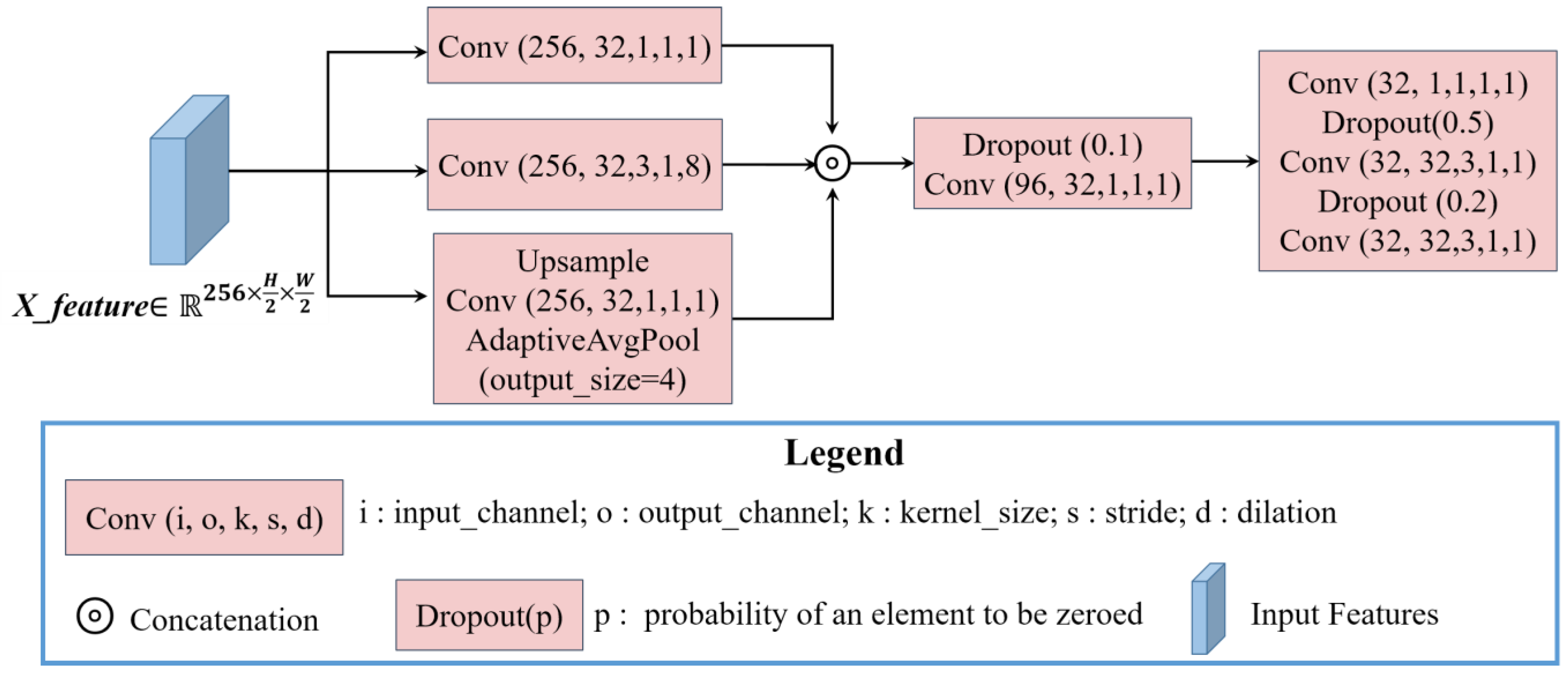Then, the channel dimension of $X_c$ is reduced from 512 to 256 by a 1 × 1 convolution layer to further reduce the computational costs for the subsequent network. The Light-ASPP module is based on ASPP in the Deeplabv3 series [40]. It takes into account the different scales of changed regions and reduces the computational costs. The architecture of the Light-ASPP module is shown in Figure 3.

In the Light-ASPP module, three parallel feature-extraction branches are formed. The input feature of the Light-ASPP module is $X\_feature\in {ℝ}^{256\times \frac{H}{2}\times \frac{W}{2}}$. The first branch is a 1 × 1 convolution layer, which retains the original information of the feature and reduces the channel dimension from 256 to 32. The second branch is a 3 × 3 atrous convolution layer with a dilation rate of 8 to capture semantic features at different scales. The third branch obtains image-level global features through an adaptive average pooling layer, a 1×1 convolution layer, and the upsample layer. After three parallel feature-extraction branches, the feature dimension is ${ℝ}^{32\times \frac{H}{2}\times \frac{W}{2}}$, and is ${ℝ}^{96\times \frac{H}{2}\times \frac{W}{2}}$ after contacting three features. Then, the output of the Light-ASPP module is obtained by three convolution layers. In addition, the dropout regularization strategy is introduced in the Light-ASPP module during training. Each convolutional layer in the Light-ASPP module is cascaded with a BN layer and a hard-swish activation function [26], which ensures detection performance and reduces computational costs. The expression of the hard-swish function is shown in Equation (2), where ReLU6 refers to the clipping of the output value of the ReLU function so that its maximum output value is 6.

$$\mathrm{hard}\_\mathrm{swish}\left(\mathrm{x}\right)=\mathrm{x}·\frac{\mathrm{ReLU}6\left(\mathrm{x}+3\right)}{6}$$

(2)

The output of the Light-ASPP module is double-upsampled, and then the pixelwise change probability map is obtained after the sigmoid layer. $CM\in {ℝ}^{1\times H\times W}$ is obtained by a fixed threshold of 0.5 during the test stage. When the pixelwise change probability is greater than 0.5, it is judged as a changed pixel. Otherwise, it is judged as unchanged.

2.3. Attention Mechanism

To enhance features of high correlation with change-detection tasks, the channel and spatial attention modules are used [9], as shown in Figure 4.

The expression of CAM is shown in Equation (3):

$$F_{out\_c}=\left[\sigma \left(\mathrm{MLP}\left(\mathrm{AvgPool}\left(F_{in\_c}\right)\right)+\mathrm{MLP}\left(\mathrm{MaxPool}\left(F_{in\_c}\right)\right)\right)\right]\times F_{in\_c}$$

(3)

$F_{in\_c}$ represents the input feature, AvgPool (∙) represents average pooling, MaxPool (∙) represents maximum pooling, MLP represents multilayer perceptron, and $\sigma \left(·\right)$ represents the hard_swish activation function. Suppose $F_{in\_c}\in {ℝ}^{C\times H\times W}$, then the dimension of $M_c^F$ is ${ℝ}^{C\times 1\times 1}$, assigning weights to each channel. The CAM is shown in Figure 4a, which is mainly divided into two steps: (1) aggregating the information of each channel and calculating the channel attention distribution of the features, that is, $M_c^F$; (2) combining $M_c^F$ with the original feature $F_{in\_c}$. The module is used after contacting $X\_edge$, $X\_1st$, and $X\_2nd$ to enhance the discriminative ability of features.

The SAM-used expression is shown in Equation (4):

$$F_{out\_s}=\left[\sigma \left(f^{7\times 7}\left(\left[AvgPool\left(F_{in\_s}\right)⊚MaxPool\left(F_{in\_s}\right)\right]\right)\right)\right]\times F_{in\_s}$$

(4)

$F_{in\_s}$ represents the input feature, $f^{7\times 7}$ represents a 7 × 7 convolutional layer, $\left[⊚\right]$ indicates a concatenation operation in the channel dimension, and the rest is the same as the CAM. Assuming that the input feature dimension $F_{in\_s}\in {ℝ}^{C\times H\times W}$, the dimension of $M_s^F$ is ${ℝ}^{1\times H\times W}$. The pixel values of each channel are assigned weights. The SAM is shown in Figure 4b, which is mainly divided into two steps: (1) aggregating the information of each pixel in the channel dimension and calculating the spatial attention distribution $M_s^F$; (2) combining $M_s^F$ with the original feature $F_{in\_s}$. SAM is applied in Layer1 to enhance the distinction between the changed area’s information and the unchanged area’s information.

2.4. Edge-Information Feature Enhancement

In the change-detection task, the performance of the edge detection of the changed areas is poor, especially for the small targets. Therefore, to pay more attention to the edge detail information and reduce the occurrence of missed detection, especially for small targets, the lightweight edge-information feature-enhancement module of the changed area is designed to improve the detection performance.

As can be seen in Figure 1, for the shallow feature $X\in {ℝ}^{24\times \frac{H}{4}\times \frac{W}{4}}$ obtained by the Input Layer, the edge-information feature $X\_edge\in {ℝ}^{128\times \frac{H}{4}\times \frac{W}{4}}$ is obtained after passing through the Edge Layer. $X\_edge$ is then used to enhance the semantic features. The Edge Layer is cascaded by three ShuffleNetV2Block basic blocks, and to avoid excessive downsampling and information loss, the spatial resolution is maintained in the Edge Layer. The edge-information feature $X\_edge$ is successively a 3 × 3 convolution layer, a 1 × 1 convolution layer, a 4 × upsample layer, and the sigmoid activation function to obtain the edge-detection output map of the changed areas. The canny operator [41] is used to process the change-detection ground truth label to obtain the edge label of changed areas, to perform supervised learning on the module.

2.5. Logit Knowledge Distillation

For the deep-learning network which is a black-box model, the “knowledge” of network learning is abstract; that is, learning how to map from the input to the output. For the change-detection task, the probability of classification as the changed class is learned by the model. The probability is a soft label relative to the 0/1 hard truth label, which reflects the probability relationship between the model to classify the image pixel into changed and unchanged classes. Therefore, the change probability generated by the large model can be used as a soft label in the training to guide the small model. That is, the large model can be used as the teacher model to transmit the learned knowledge information to the small model [29]. It helps achieve better detection performance with a smaller model.

3M-CDNet [34] is used as the teacher network to distill Shuffle-CDNet. Because of the difference in the structure of the two networks, logit distillation is used. That is, the probability distribution of the outputs of the two networks is directly matched. The activation function of both networks’ output layers is the sigmoid function, and the expression is shown in Equation (5):

$$f\left(x\right)=\frac{1}{1+e^{-x}}$$

(5)

The output of the teacher network and the student network through the sigmoid function are “softened” during the training process; that is, the temperature coefficient $T$ is introduced. The modified nonlinear activation function is shown in Equation (6):

$$f_T\left(x\right)=\frac{1}{1+e^{-\frac{x}{T}}}$$

(6)

$T$ is set to 1 during the student network test, so that the results learned by the student network are as close as possible to the results of the teacher network.

In the experiment, the knowledge distillation strategy was used on the LEVIR-CD dataset and the season-varying dataset to distill the student network Shuff-CDNet with the teacher network 3M-CDNet for training. On the SYSU-CD dataset, the detection performance of the Shuffle-CDNet is already better than that of the 3M-CDNet after the adoption of the specific data-augmentation strategy, so the knowledge-distillation strategy is no longer used.

3. Experiment Settings

3.1. Training Datasets

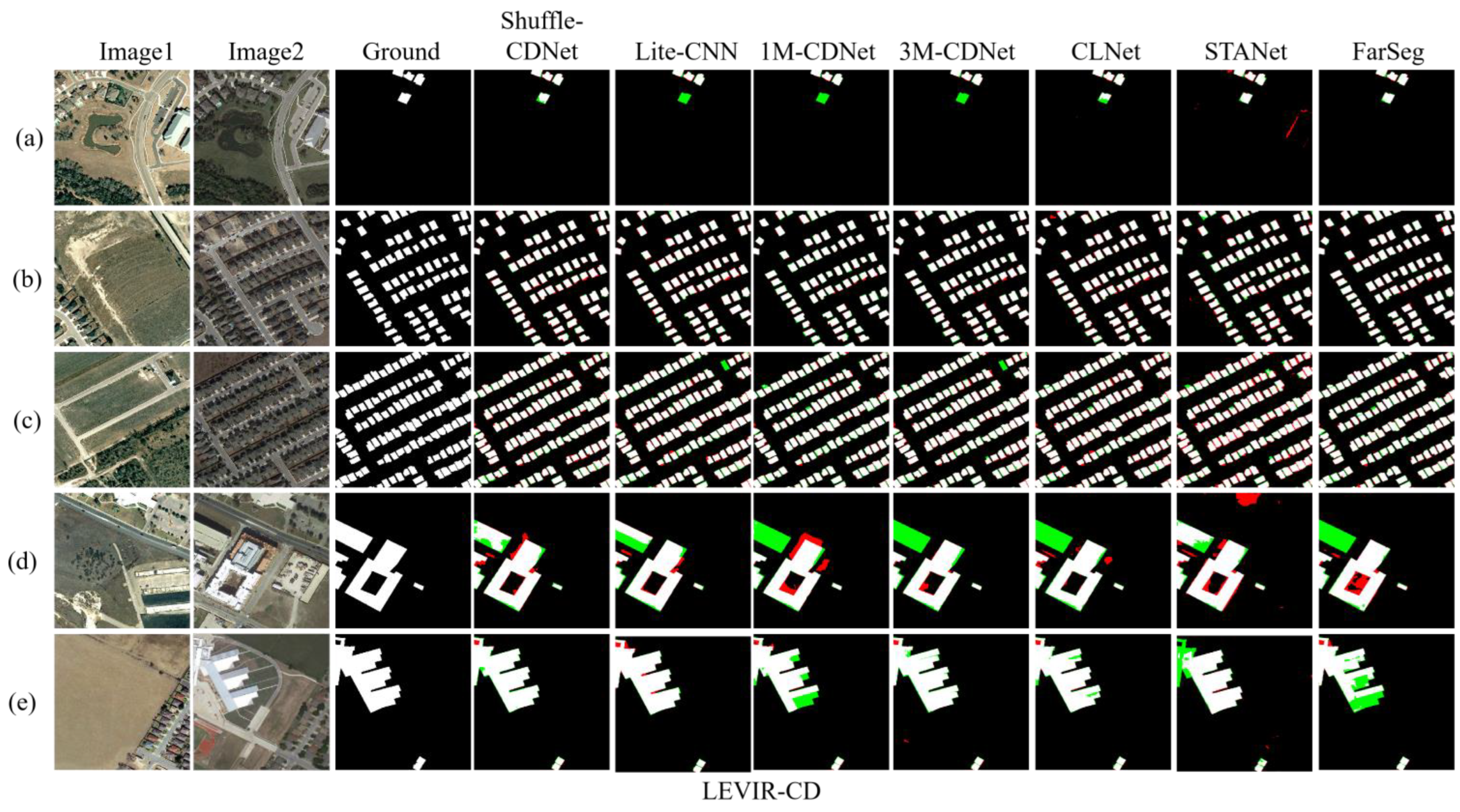
In the experiment, Shuffle-CDNet was evaluated on three publicly available change-detection remote-sensing image datasets, including LEVIR-CD [14], season-varying [42], and SYSU-CD [43] datasets.

(1) LEVIR-CD dataset: It contains 637 pairs of two-phase optical satellite remote-sensing images of building changes collected from the Google Earth platform. Each remote-sensing image contained three bands of RGB, with a spatial resolution of 0.5 m/pixel, and the period of the two phases of images ranged from 5 to 14 years. The types of building changes mainly involve the new construction and demolition of buildings. It is randomly divided into three parts: 70% for the training set, 10% for the validation set, and 20% for the test set. The 512 × 512 sliding windows with a stride of 256 are used to crop the original image to 512 × 512 image slices.

(2) Season-varying dataset: It contains 7 pairs of remote-sensing images of seasonal changes taken from Google Earth, each with an original size of 4725 × 2700. The spatial resolution ranges from 3–100 cm/pixel. The seasonal differences between the two phases of the image are significant, mainly reflecting the changes in buildings, roads, vehicles, and other features, ignoring the changes brought about by seasonal changes (e.g., vegetation growth and wilting, snow-covered ground). The dataset author cropped the original image into image slices of 256 × 256, enhanced by random rotation within 360°, resulting in a total of 16,000 pairs of image slices. Ultimately, it is divided in a way consistent with the original paper: 10,000 pairs of samples as the training set, 3000 pairs as the validation set, and the remaining 3000 pairs as the test set.

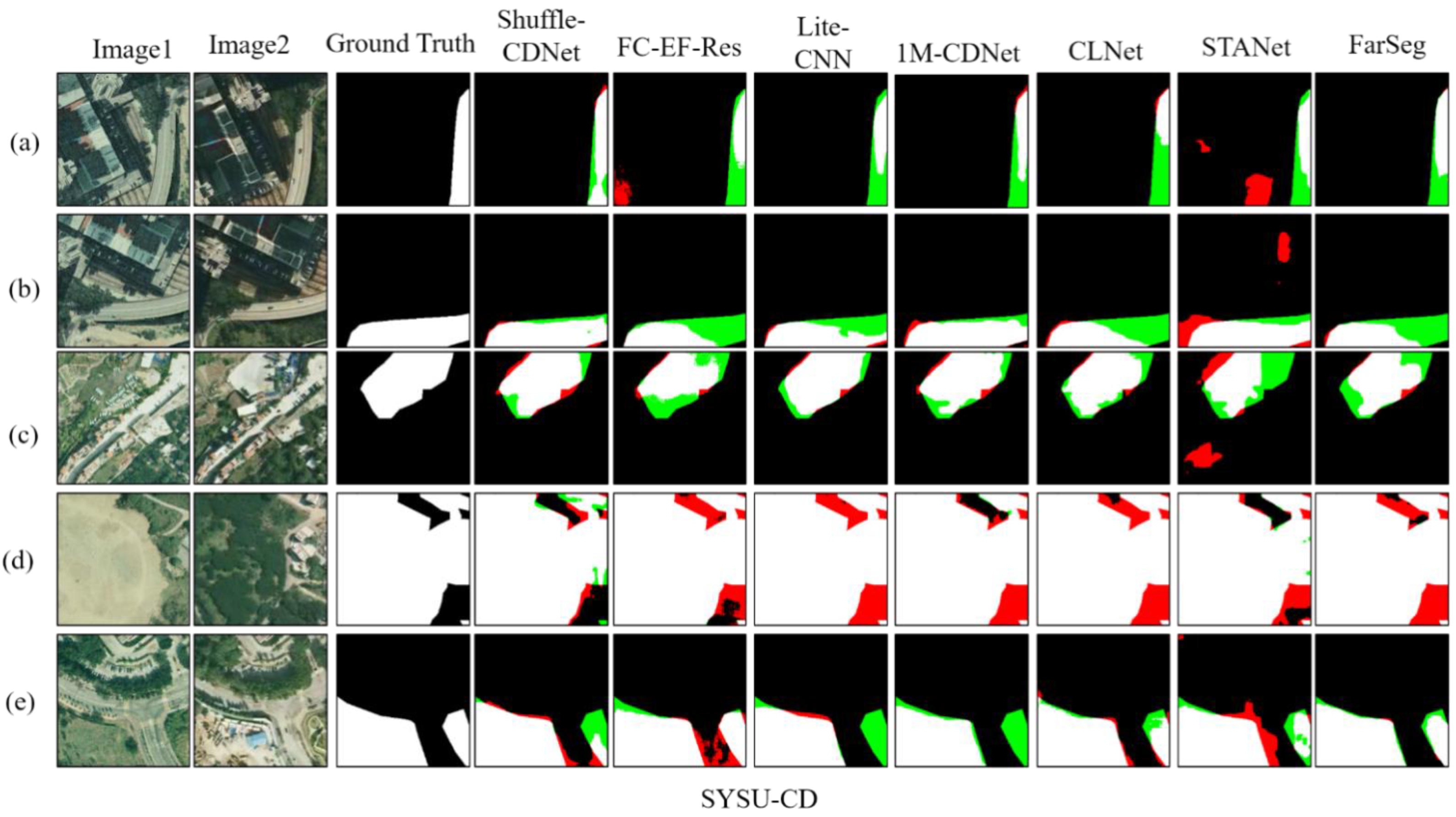
(3) SYSU-CD dataset: It contains 20,000 pairs of aerial images with a resolution of 0.5m, reflecting the rich changes in buildings, especially high-rise buildings in Hong Kong, China, and port-related change information between 2007 and 2014. The main types of changes include new urban buildings, suburban expansion, preconstruction foundations, vegetation changes, road expansion, and offshore construction. The 20,000 pairs of datasets are randomly divided into training, validation, and testing sets in a 6:2:2 ratio.

3.2. Implementation Details

Shuffle-CDNet was implemented based on the Pytorch framework [44]. The model training was performed using the AdamW optimizer [45] with ${\beta }_1=0.9$ and ${\beta }_2=0.99$, of which the initial learning rate and weight decay were empirically set to 0.000125 and 0.0005, respectively. It was trained without pretrained models on a single NVIDIA RTX 3090 GPU. The batch size of the training was set to 16. The training epochs were set to 400, 900, and 250 for LEVIR-CD, season-varying, and SYSU-CD datasets, respectively.

3.3. Data Augmentation

Online data augmentation (DA) was used to simulate scale changes, light changes, and pseudo-variations. After loading each batch of data, online DA is applied randomly with a probability of 0.8 through random movement, rotation, scaling, horizontal and vertical flipping, and changing the spectral feature strategy. Each DA method is randomly applied with a probability of 0.5.

Moreover, according to the qualitative analysis of the datasets, the spectral difference between the prephase and postphase images of the LEVIR-CD dataset and the season-varying dataset is relatively large, but it is relatively small for the SYSU-CD dataset. Therefore, the specific DA strategy of switching the channel order when contacting the prephase and postphase images as the input $I^{\left(1,2\right)}\in {ℝ}^{6\times H\times W}$ is adopted with a probability of 0.25 for the SYSU-CD dataset.

3.4. Loss Function

The loss function consists of three parts weighted, and the expression is shown in Equation (7):

$$L_{total}=\alpha L_{cd}+\beta L_{edge}+\gamma L_{kd}$$

(7)

The first part of the loss function $L_{cd}$ consists of the standard binary cross-entropy loss function and the Tversky loss function weighted, as shown in equations (8).

$$\begin{array}{cc}& L_{cd}={\alpha }_1{l}_{bce}+{\alpha }_2{l}_{tversky}\\ & l_{bce}=-\frac{1}{N}{\displaystyle {\displaystyle \sum }_{n=1}^N}\left(y_n\log \left({\widehat{y}}_n\right)+\left(1-y_n\right)\log \left(1-{\widehat{y}}_n\right)\right)\\ & l_{tversky}=1-\frac{1}{N}{\displaystyle {\displaystyle \sum }_{n=1}^N}\frac{y_n{\widehat{y}}_n}{y_n{\widehat{y}}_n+{\alpha }_{21}(1-y_n){\widehat{y}}_n+{\alpha }_{22}{y}_n\left(1-{\widehat{y}}_n\right)}\end{array}$$

(8)

$y_n$ (1/0) represents a changed pixel or an unchanged pixel in the truth label, and ${\widehat{y}}_n$ represents the probability that the pixels in the prediction image belong to the changed class. When ${\alpha }_{21}={\alpha }_{22}=1$, the Tversky loss is the Jaccard loss [34]. Due to the problem of sample imbalance in the change-detection task, the number of unchanged pixels is much greater than the number of changed pixels. Therefore, to avoid some changed pixels being mistakenly judged as unchanged pixels, the Tversky loss hyperparameter ${\alpha }_{21}=0.3$ and ${\alpha }_{22}=0.7$ are set in the experiments. That is, the weight ratio of false negative (FN) is increased. The goal is to balance the recall and the precision rate and improve the F1 coefficient of the detection results. The hyperparameters ${\alpha }_1$ and ${\alpha }_2$ in $L_{cd}$ are set to 0.3 and 0.7, respectively. It increases the weight ratio of the Tversky loss in the $L_{cd}$ loss function.

The second part of the loss function $L_{edge}$ is the standard binary cross-entropy loss function. It is aimed at the edge-information feature-enhancement module. The prediction is the edge-detection output map of the changed areas, and the true label is the edge label of the changed areas extracted by the canny operator. The third part of the loss function $L_{kd}$ is the standard binary cross-entropy loss function, which is for the logit distillation module. The prediction is the prediction output of the student network Shuffle-CDNet, and the true label is the prediction output of the teacher network 3M-CDNet. The hyperparameters of the loss weights of each part are set in the $L_{total}$ $\alpha =1$,$\mathsf{\beta }=0.5$, and $\mathsf{\gamma }=25$, respectively. It is worth noting that for the SYSU-CD dataset, the $L_{total}$ does not contain $L_{kd}$ because no knowledge-distillation strategy was used.

3.5. Evaluation Metrics

F1-Score (F1), intersection over union (IoU), precision rate (Pr), recall rate (Re), and overall accuracy (OA) are mainly used as evaluation metrics, as shown in Equation (9):

$$\begin{array}{cc}\mathrm{Pr}=\frac{\mathrm{TP}}{\mathrm{TP}+\mathrm{FP}}& \\ \mathrm{Re}=\frac{\mathrm{TP}}{\mathrm{TP}+\mathrm{FN}}& \\ \mathrm{OA}=\frac{\mathrm{TP}+\mathrm{TN}}{\mathrm{TP}+\mathrm{FP}+\mathrm{TN}+\mathrm{FN}}& \\ \mathrm{IoU}=\frac{\mathrm{TP}}{\mathrm{TP}+\mathrm{FP}+\mathrm{FN}}& \\ \mathrm{F}1=\frac{2\times \mathrm{Pr}\times \mathrm{Re}}{\mathrm{Pr}+\mathrm{Re}}& \end{array}$$

(9)

TP, TN, FP, and FN, respectively, mean true positive, true negative, false positive, and false negative. IoU and F1 are comprehensive evaluation metrics. The larger the evaluation metric value, the better the comprehensive performance of the model.

4. Results

In order to compare with the proposed Shuffle-CDNet on different datasets, several state-of-the-art deep-learning-based methods were selected for comparative experiments. These methods includes pure convolutional-network-based approaches: FC-Siam-Diff [8], FC-Siam-Conc [8], FC-Siam-Res [46], and CLNet [11]; Attention-based approaches: STANet [14] and FarSeg [47], Transformer-based approaches: BIT-CD [18], and lightweight networks for remote-sensing images: MSPP-Net [32], Lite-CNN [33], 1M-CDNet, and 3M-CDNet [34].

4.1. Computational Efficiency

Table 1. Comparison of network parameters, computational costs, and inference time.

Method	Number of Parameters (M)	Computational Costs (GFLOPs) w/bs = 1		Inference Time (ms) w/bs = 16
		512 × 512	256 × 256	512 × 512	256 × 256
FC-Siam-Diff	1.35	20.74	5.18	130.75	32.05
FC-Siam-Conc	1.55	20.75	5.19	133.09	32.12
FC-EF-Res	1.10	6.94	1.73	92.35	23.54
MSPP-Net	6.25	66.16	16.54	190.85	47.09
Lite-CNN	3.88	19.17	4.79	117.98	29.38
1M-CDNet	1.26	18.43	4.61	128.76	33.62
3M-CDNet	3.12	94.83	23.71	336.87	55.28
CLNet	8.53	35.65	8.91	130.87	33.01
STANet	16.93	206.68	32.42	-	-
FarSeg	31.38	47.45	11.86	171.14	44.38
BIT-CD	3.05	62.68	15.67	264.56	64.67
Shuffle-CDNet	0.71	12.52	3.13	123.10	31.60

lists the number of parameters (M), the computational costs (GFLOPs), and the inference time (ms) of different methods. FLOPs represent the number of floating-point operations and $1\mathrm{GFLOPs}={10}^9\mathrm{FLOPs}$. Tests based on Table 1 were performed on an NVIDIA RTX 2080Ti GPU with 11 GB of memory. The fixed 1 × 6 × 512 × 512 and 1 × 6 × 256 × 256 image sizes were used as inputs when testing the computational costs. The fixed 16 × 6 × 512 × 512 and 16 × 6 × 256 × 256 image sizes were used as inputs to make full use of GPU memory capacity when testing the inference time and improve the inference efficiency. The average time of 1000 forward inferences using randomly generated test samples was used as the inference time to reduce the test error. “-” indicates that the STANet requires a large amount of memory and cannot be run on a single GPU.

As can be seen from Table 1, the parameters of Shuffle-CDNet are only 0.71 M, which is 0.55 M lower than 1M-CDNet. It is the lowest among all networks. For the computational costs, Shuffle-CDNet has 12.52 GFLOPs and 3.13 GFLOPs in the input image size of 1 × 6 × 512 × 512 and 1 × 6 × 256 × 256, respectively, which is 5.91 G and 1.48 GFLOPs lower than 1M-CDNet. It is second only to the FC-EF-Res in all comparison networks. However, the computational costs cannot directly reflect the inference time. The latter is also affected by other factors such as the degree of parallelism and the memory access cost [28], so the inference time should be directly tested on the target computing platform. For the inference time, the inference time of Shuffle-CDNet is 123.10 ms and 31.60 ms for the input size of 16 × 6 × 512 × 512 and 16 × 6 × 256 × 256, respectively. It is 5.56 ms and 2.02 ms lower than 1M-CDNet, respectively, which has a clear advantage in inference time after FC-EF-Res and Lite-CNN in all comparison networks. Compared with Lite-CNN, the computational costs of Shuffle-CDNet are significantly lower than that of the former, but the inference time is greater, because the degree of parallelism of Lite-CNN is better than that of Shuffle-CDNet. Shuffle-CDNet uses edge-information feature enhancement and two-stage feature-fusion strategy to balance the degree of network parallelism and detection performance.

4.2. Comparisons on LEVIR-CD Dataset

(a)

Quantitative evaluation

Table 2. Comparison results on the LEVIR-CD dataset.

Method	Pr (%)	Re (%)	OA (%)	IoU	F1
FC-Siam-Diff	91.25	88.18	98.97	81.30	89.69
FC-Siam-Conc	89.49	89.18	98.92	80.72	89.33
FC-EF-Res	91.48	88.04	98.97	81.37	89.73
MSPP-Net	89.65	86.73	98.81	78.83	88.16
Lite-CNN	90.77	89.96	99.02	82.42	90.36
1M-CDNet	92.32	90.06	99.11	83.79	91.18
3M-CDNet	91.99	91.24	99.15	84.52	91.61
CLNet	90.85	90.53	99.05	82.97	90.69
STANet	85.01	91.38	98.74	78.69	88.08
FarSeg	91.04	90.22	99.05	82.86	90.63
BIT-CD	90.38	89.69	98.99	81.87	90.03
Shuffle-CDNet	91.41	91.08	99.11	83.90	91.25

lists the experimental results for quantitative comparison of the LEVIR-CD dataset. Compared with 1M-CDNet, Shuffle-CDNet increased by 0.07% on the F1 metric and 0.11% on the IoU metric. As available from Table 1, the Shuffle-CDNet has computational costs of 12.52 GFLOPs when the input image size is 1 × 6 × 512 × 512, which is only about 68% of 1M-CDNet. Compared with the teacher model 3M-CDNet in the logit distillation training, F1 and IoU metrics of the student model Shuffle-CDNet are a little lower than the former, but the computational costs of the latter are only about 13% of the former, and the inference time of the latter is only about 36% of the former, which greatly improves the detection efficiency. Compared with the baseline STANet and BIT-CD, Shuffle-CDNet increased by 3.17% and 1.22% on the F1, respectively, and by 5.21% and 2.03% on the IoU, respectively. As available from Table 1, Shuffle-CDNet has only about 20% of the computational costs of the BIT-CD. For other lightweight networks, Shuffle-CDNet increased the computational costs and inference time a little higher than that of the FC-EF-Res, but the former increased by 1.52% and 2.53% respectively in F1 and IoU; Shuffle-CDNet increased by 3.09% and 0.89% on F1 compared with MSPP-Net and Lite-CNN networks, respectively. The IoU also improves by 5.07% and 1.48%, respectively. Combined with the metrics, it can be seen that the Shuffle-CDNet has the best balance between computational costs and detection performance.

(b)

Qualitative evaluation

For visual comparison, Figure 5 shows the detection results on the LEVIR-CD test sets. Black, white, red, and green pixels represent TN, TP, FP, and FN, respectively. It can be seen that Shuffle-CDNet can reduce missing detection of small changed objects, mainly due to the edge-information feature-enhancement module. For example, in Figure 5a–c, Shuffle-CDNet is clearly improved with regard to the missed detection phenomenon of small objects compared with other CNN-based networks such as Lite-CNN and 1M-CDNet. Attention-based networks such as STANet and FarSeg, as well as CLNet, take contextual information into account and perform well in small-object detection. However, for the detection of large-range changed areas, as shown in Figure 5d,e, Shuffle-CDNet can generate a change map with better changed regional internal compactness compared to other networks including 3M-CDNet. It can be seen that the qualitative results are consistent with the analysis of the quantitative results, and Shuffle-CDNet performs better than other advanced networks on the LEVIR-CD dataset.

4.3. Comparisons on Season-Varying Dataset

(a)

Quantitative evaluation

Table 3. Comparison results on the season-varying dataset.

Method	Pr (%)	Re (%)	OA (%)	IoU	F1
FC-Siam-Diff	93.98	81.05	97.02	77.05	87.04
FC-Siam-Conc	91.94	82.06	96.90	76.56	86.72
FC-EF-Res	89.91	87.37	97.25	79.56	88.62
MSPP-Net	92.95	85.93	97.46	80.67	89.30
Lite-CNN	96.58	89.76	98.34	87.00	93.05
1M-CDNet	95.05	98.61	99.19	93.79	96.80
3M-CDNet	95.88	99.16	99.37	95.10	97.49
CLNet	98.62	94.46	99.15	93.23	96.50
STANet	93.13	93.59	98.36	87.55	93.36
FarSeg	95.12	98.13	99.15	93.43	96.60
BIT-CD	98.49	92.34	98.88	91.05	95.31
Shuffle-CDNet	95.54	98.01	99.19	93.73	96.76

lists results on the season-varying dataset, which has some pseudo-variational interference due to seasonal variations. Shuffle-CDNet still performs well on comprehensive metrics such as F1 and IoU compared to most other detection networks. For example, compared with the FarSeg, Shuffle-CDNet has increased by 0.16% and 0.30% on the F1 and IoU, respectively. It can be obtained from Table 1 that when the network input image size is 1 × 6 × 256 × 256, the computational costs of Shuffle-CDNet are only 26% of FarSeg. Compared with lightweight networks, Shuffle-CDNet is superior to FC-Siam-Conc, FC-Siam-Diff, and MSPP-Net in terms of computational costs, inference time, and metrics F1 and IoU. Compared with FC-EF-Res and Lite-CNN, although it is slightly better than shuffle-CDNet in terms of computational costs or inference time, Shuffle-CDNet is 8.14% and 3.71% higher than the FC-EF-Res and Lite-CNN networks on F1 metric, and the IoU metric is increased by 14.17% and 6.73% respectively, which is a significant improvement. Compared to 1M-CDNet, Shuffle-CDNet achieves nearly equal detection performance with lower computational costs and faster inference time.

(b)

Qualitative evaluation

Figure 6 shows the results of different methods on the season-varying test sets. In terms of test results, Shuffle-CDNet is significantly superior to CNN-based networks such as FC-EF-Res and Lite-CNN networks. From Figure 6d,e, it can be seen that for the change detection of dense small objects or slender areas, Shuffle-CDNet has better performance than 1M-CDNet, STANet, and FarSeg networks, especially with better boundary-detection performance. Shuffle-CDNet can better maintain the independence of the detected area and can achieve a detection effect similar to that of the 1M-CDNet network with lower computational costs. The qualitative analysis is consistent with the quantitative results.

4.4. Comparisons on SYSU-CD Dataset

(a)

Quantitative evaluation

Table 4. Comparison results on the SYSU-CD dataset.

Method	Pr (%)	Re (%)	OA (%)	IoU (%)	F1 (%)
FC-Siam-Diff	89.13	61.08	89.06	56.84	72.48
FC-Siam-Conc	81.95	77.05	90.59	65.87	79.42
FC-EF-Res	81.08	78.33	90.58	66.22	79.68
MSPP-Net	75.86	78.40	89.02	62.75	77.11
Lite-CNN	79.80	82.18	90.89	68.03	80.98
1M-CDNet	80.73	81.55	91.06	68.26	81.14
3M-CDNet	80.78	82.16	91.18	68.73	81.47
CLNet	82.64	79.08	91.15	67.81	80.82
STANet	73.53	82.49	88.87	63.60	77.75
FarSeg	84.03	78.45	91.40	68.28	81.15
BIT-CD	83.18	72.92	90.14	63.56	77.72
Shuffle-CDNet	80.93	82.14	91.22	68.82	81.53

lists the results of the SYSU-CD dataset. It can be seen that the F1 and IoU metrics of Shuffle-CDNet are better than other methods. For example, compared with the FarSeg network, Shuffle-CDNet improves by 0.38% and 0.54% on F1 and IoU metrics, respectively. Compared with the 1M-CDNet method, Shuffle-CDNet improves by 0.39% and 0.56% on the F1 and IoU. Especially for 3M-CDNet, Shuffle-CDNet also improves by 0.06% and 0.09% on the F1 and IoU indicators, respectively. From Table 1, when the input image size is 1 × 6 × 256 × 256, the computational costs and inference time of the Shuffle-CDNet network are also much smaller than that of 3M-CDNet.

(b)

Qualitative evaluation

Figure 7 shows the detection results of different methods on the SYSU-CD test sets.

The SYSU-CD dataset has more large-scale variation areas, such as Figure 7d,e images; it can be seen that in the test results of the Shuffle-CDNet network compared to other CNN-based networks such as FC-EF-Res and 1M-CDNet, as well as lightweight networks Lite-CNN, more false detections are clearly avoided. At the same time, CLNet and STANet also perform relatively well on the Figure 7d,e images, but there are more missed detections on the Figure 7a–c images compared with the Shuffle-CDNet network. In particular, the STANet network has more false detections. Therefore, overall, Shuffle-CDNet has better detection performance on the SYSU-CD dataset, which is consistent with the quantitative-analysis results.

4.5. Ablation Studies

The effects of the two-level feature-fusion strategy, edge-information feature-enhancement module, logit distillation module, Tversky loss, and attention mechanism on the performance of Shuffle-CDNet were verified by ablation experiments.

Table 5. Effects of two-level feature-fusion strategy.

Methods	LEVIR-CD			Season-Varying			SYSU-CD
	OA	IoU	F1	OA	IoU	F1	OA	IoU	F1
w/o two-level	99.09	83.52	91.02	99.14	93.32	96.54	90.93	67.86	80.86
w/two-level	99.11	83.90	91.25	99.19	93.73	96.76	91.22	68.82	81.53

,

Table 6. Effects of edge-information feature-enhancement module.

Methods	LEVIR-CD			Season-Varying			SYSU-CD
	OA	IoU	F1	OA	IoU	F1	OA	IoU	F1
w/o edge	99.09	83.60	91.07	99.10	93.06	96.41	91.10	68.85	81.55
w/edge	99.11	83.90	91.25	99.19	93.73	96.76	91.22	68.82	81.53

,

Table 7. Effects of logit distillation.

Methods	LEVIR-CD			Season-Varying
	OA	IoU	F1	OA	IoU	F1
w/o kd	99.08	83.36	90.93	98.94	91.98	95.82
w/kd	99.11	83.90	91.25	99.19	93.73	96.76

,

Table 8. Effects of Tversky loss.

Datasets	Methods	Pr	Re	OA	IoU	F1
LEVIR-CD	w/o Tversky loss	91.99	90.12	99.10	83.56	91.04
	w/Tversky loss	91.41	91.08	99.11	83.90	91.25
Season-Varying	w/o Tversky loss	94.68	98.34	99.11	93.18	96.47
	w/Tversky loss	95.54	98.01	99.19	93.73	96.76
SYSU-CD	w/o Tversky loss	82.53	79.41	91.18	67.99	80.94
	w/Tversky loss	80.93	82.14	91.22	68.82	81.53

and

Table 9. Effects of attention mechanism.

Methods	LEVIR-CD			Season-Varying			SYSU-CD
	OA	IoU	F1	OA	IoU	F1	OA	IoU	F1
w/o attention	99.09	83.47	90.99	99.04	92.57	96.14	90.92	67.86	80.86
w/attention	99.11	83.90	91.25	99.19	93.73	96.76	91.22	68.82	81.53

list the results of ablation experiments on the LEVIR-CD, season-varying, and SYSU-CD datasets, where “w/” and “w/o” mean “with” and “without”, respectively. All data in the tables are in percentage form.

4.5.1. Effectiveness of Two-Level Feature-Fusion Strategy

Table 5 shows that when the two-stage fusion strategy is adopted, the fusion of edge-information features $X\_edge$, low-level features $X\_1st$, and high-level features $X\_2nd$ (w/two-level) is used to achieve better detection performance on three datasets than only the use of $X\_edge$ and $X\_2nd$. feature fusion (w/o two-level). F1 increases by 0.23%, 0.22%, and 0.67% on the LEVIR-CD, season-varying, and SYSU-CD datasets, respectively. IoU increases by 0.38%, 0.41%, and 0.96%, respectively. It can be seen that this strategy can improve detection performance, supply more detailed information, and balance the computational costs and detection performance.

4.5.2. Effectiveness of Edge-Information Feature-Enhancement Module

Table 6 shows that the introduction of the edge-information feature-enhancement module (w/edge) achieved better detection performance than without introduction (w/o edge) on the LEVIR-CD and the season-varying datasets. F1 increases by 0.18% and 0.35% on the LEVIR-CD and season-varying datasets, respectively, and IoU increases by 0.30% and 0.67%, respectively. However, on the SYSU-CD dataset, it can be seen that this module cannot work well, because there are many dense small changed areas for the LEVIR-CD and season-varying datasets, but the labeled changed areas of the SYSU-CD dataset are mostly large-scale, while this module can mainly help to improve the detection performance of the small-scale changed areas and especially improve missed detection for small targets.

The qualitative results of the ablation experiment of this on LEVIR-CD and season-varying datasets are shown in Figure 8. It can be seen that especially for the detection of the small changed targets, this module can improve the detection performance for small targets and edge areas of changed regions and improve the detection performance. It is consistent with the quantitative-analysis results in Table 6.

4.5.3. Effectiveness of Logit Distillation

Table 7 shows that the introduction of the logit knowledge-distillation module (w/kd) has achieved a significant improvement in quantitative metrics compared with direct training (w/o kd) on the LEVIR-CD and season-varying datasets. F1 increases by 0.32% and 0.94% on the LEVIR-CD and season-varying datasets, respectively, and IoU increases by 0.54% and 1.75%, respectively. When the logit distillation module is introduced, in the process of training Shuffle-CDNet as the student network, the information learned by 3M-CDNet is introduced, which improves the training effect.

4.5.4. Effectiveness of Tversky Loss

As can be seen from Table 8, after the introduction of the Tversky loss (w/Tversky loss), compared with the use of only the binary cross-entropy loss function in $L_{cd}$ (w/o Tversky loss), the performance improvement was achieved in metrics. F1 increases by 0.21%, 0.29%, and 0.59% on the LEVIR-CD, season-varying, and SYSU-CD datasets, respectively, and IoU increases by 0.34%, 0.55%, and 0.83%, respectively. After the introduction of Tversky loss, the Pr and Re metrics are relatively more balanced, which is why the F1 metric can be improved.

4.5.5. Effectiveness of Attention Mechanism

As can be seen from Table 9, when CAM and SAM (w/attention) are introduced, F1 increases by 0.26%, 0.62%, and 0.67% on the LEVIR-CD, season-varying, and SYSU-CD datasets, respectively. IoU increases by 0.43%, 1.16%, and 0.96%, respectively. When the attention mechanism module is introduced, the features with high correlation with the change-detection task are enhanced, and the distinction between the changed area information and the unchanged area information is enhanced. As a result, the performance of Shuffle-CD is significantly improved.

5. Discussion

In this study, we proposed the lightweight network named Shuffle-CDNet for change-detection tasks. The quantitative and qualitative results on three datasets have confirmed that Shuffle-CDNet can achieve a better balance in computational efficiency and detection performance. The lightweight network meets the current practical application requirements [48].

The proposed method mainly consists of the backbone network and the classifier. The building blocks of ShuffleNet v2 [28] are adopted to form the backbone network. It introduces channel shuffle and depthwise separable convolution operations to reduce the computational costs without sacrificing network accuracy. The idea of the ShuffleNet v2 is also used in other applications such as forest-fire recognition [49], which also adopts channel-shuffle operation. At the same time, the depth and width of the proposed network are reduced greatly, with the channels of the final output feature of the proposed backbone being 256 but 512 for 3M-CDNet [34]. Compared with other advanced methods, for example, BIT-CD [18] and SwinSUNet [21] adopt transformers in the backbone network, 3M-CDNet [34] adopts the deformable convolution, STANet [14] adopts complex attention mechanisms, and Peng et al. [12] proposed the method based on UNet++ with dense skip connections. These operations increase computational costs. We can see from Table 1 that the inference time of Shuffle-CDNet is about 47% of BIT-CD and about 37% of 3M-CDNet. But from Table 2, Table 3 and Table 4, Shuffle-CDNet performs better than BIT-CD. For example, it increases F1 (1.22%) and IoU (2.03%) metrics on the LEVIR-CD dataset compared to BIT-CD. Shuffle-CDNet achieves nearly equal detection performance compared to 3M-CDNet with lower computational costs and faster inference time. It even improves the F1 (0.06%) and IoU (0.09%) metrics on the SYSU-CD dataset compared to 3M-CDNet. The Light-ASPP module is adopted to utilize the multilevel features in the classifier. Multilevel feature aggregation is important for change detection such as AGCDetNet [15], which introduces the attention module in the ASPP module. Some operations are also adopted to balance computational efficiency and performance. The lightweight edge-information feature-enhancement module is introduced and edge constraint is adopted in the loss function since downsampling operations could lose spatial details. It helps to improve the edge detection, especially for small changed regions, which is consistent with other studies such as EANet [37] and EPUNet [35]. Compared with EPUNet, which adopts UNet architecture, Shuffle-CDNet adopts the building block of ShuffleNet v2 as the basic block in this module, which can reduce the computational costs. The edge information is rarely considered in lightweight missions such as MSPP-Net [32], Lite-CNN [33] and 1M-CDNet [34]. From Table 1, Table 2, Table 3 and Table 4, Shuffle-CDNet improves performance greatly compared to MSPP-Net and Lite-CNN with even faster inference time than MSPP-Net. Compared with these lightweight methods, Shuffle-CDNet adopts concise channel attention and spatial attention modules to enhance the features associated with the changed areas. It can capture long-range contextual information. This idea is consistent with other methods such as CLNet [11], FarSeg [47] and IFN [9], but it is different from IFN [9] and AGCDetNet [15], in that Shuffle-CDNet does not use dense attention modules to improve the computational efficiency while the former two methods use attention modules in more positions. From Table 1, Table 2, Table 3 and Table 4, Shuffle-CDNet improves F1 and IoU metrics compared to CLNet and FarSeg with lower computational costs on three datasets. For example, Shuffle-CDNet improves F1 (0.56%) and IoU (0.93%) metrics on the LEVIR-CD dataset compared to CLNet. Furthermore, the proposed method introduces knowledge distillation in change-detection tasks, which was almost absent in previous research and could effectively improve detection performance. However, knowledge distillation is used widely in speech recognition [50], scene classification [51], and other tasks. It is a general idea and we have migrated well to the change-detection tasks. Because of those operations, the Shuffle-CDNet still perform well under the condition of lower computation costs. As we can see in Table 2, Table 3 and Table 4, Shuffle-CDNet obtains a better performance than most of other methods with better computational efficiency.

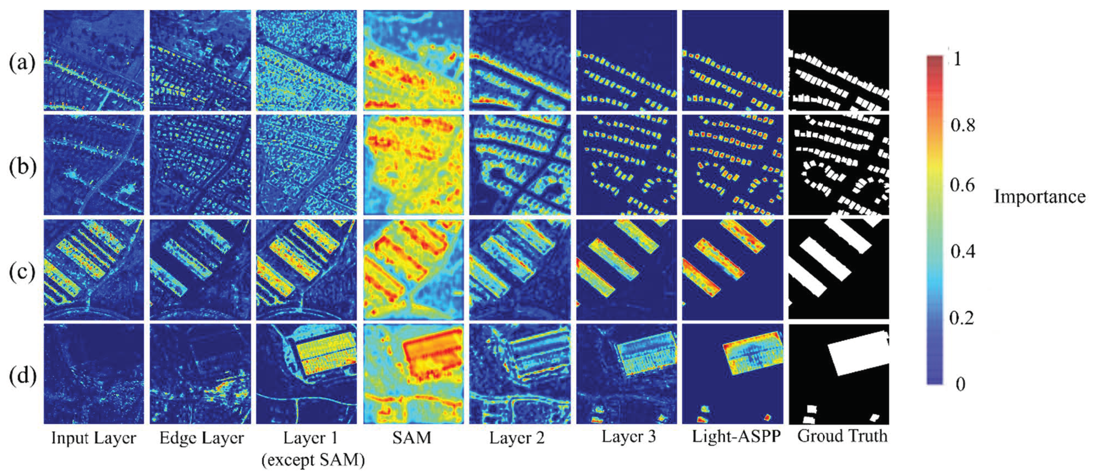
Taking the LEVIR-CD dataset as an example, the Grad-CAM visualization method [52,53] is used to visually analyze the key layers and modules of the Shuffle-CDNet network. The Grad-CAM method uses the gradients of the changed regions to produce heatmaps showing the relevance for the decision of individual pixels and highlighting the important regions. The results are shown in Figure 9.

If the area is closer to red, it means that the area of the features generated by the modules is more important to the change-detection task. If the area is closer to blue, the opposite is true. It can be seen that the shallow features of Shuffle-CDNet can be obtained through the Input Layer, and then the edge-information features can be obtained through the Edge Layer. The SAM module can enhance the pixel-level features related to change detection in the spatial domain, and then the deep features of the network can be gradually obtained. As can be seen from Figure 9d, for some large-scale changed areas, the relevant features cannot be well-extracted after passing through the Input Layer, so the edge information of the large-scale changed areas cannot be featured after the Edge Layer. This is also the reason why the edge-information feature-enhancement module has a poor effect on the SYSU-CD dataset containing more large-scale changed areas. The network visualization also reflects the rationality and effectiveness of the Shuffle-CDNet structure. In the future, it will be necessary to solve the problem of edge-information fusion in large-scale changed areas. Moreover, a neural architecture search (NAS) [54] and model pruning [55] will be tried to further reduce the computational costs and the inference time of the network, and improve the detection performance.

6. Conclusions

In order to reduce computational costs and reduce the inference time of the network, a lightweight network structure Shuffle-CDNet is proposed for the change-detection task of remote-sensing images in this paper. In the backbone, the building blocks of ShuffleNet v2 are adopted. The channel shuffle and depthwise separable convolution operation are integrated, and the depth and width of the backbone network are greatly reduced. In addition, the Light-ASPP module is designed to consider the global information and local context information to detect the binary change-detection output. In addition, to balance the network computation, inference time, and detection performance, the lightweight edge-information feature-enhancement module is designed to integrate with the shallow and deep features of the backbone network. This can improve the edge-detection performance of Shuffle-CDNet, especially for the small changed targets. The SAM and CAM are introduced to improve the feature expression ability and suppress the feature information unrelated to the change-detection task. The logit knowledge-distillation strategy is adopted on the LEVIR-CD and season-varying datasets. 3M-CDNet was used as the teacher network to provide more supervisory information for Shuffle-CDNet during the training phase. The data-augmentation strategy of randomly switching the channel order of the original image is adopted on the SYSU-CD dataset to improve the detection performance

A large number of comparative experiments have verified the effectiveness of Shuffle-CDNet. Experimental results show that compared with other current advanced methods, Shuffle-CDNet greatly reduces the computational costs without sacrificing network accuracy, even if comprehensive metrics F1 and IoU are higher than most other networks. Additionally, the inference time of Shuffle-CDNet also occupies an advantage, improving efficiency. For example, the F1 and IoU metrics of Shuffle-CDNet reached 0.9125 and 0.8390 on the LEVIR-CD dataset, 0.9676 and 0.9373 on the season-varying dataset, and 0.8153 and 0.6882 on the SYSU-CD dataset, respectively. The ablation studies and network visualization results also illustrate the effectiveness and rationality of the design of the Shuffle-CD network. On the whole, Shuffle-CDNet balances the computational costs and detection performance well and improves the detection efficiency of the network.