Ensemble Machine Learning of Random Forest, AdaBoost and XGBoost for Vertical Total Electron Content Forecasting

Abstract

Space weather describes varying conditions between the Sun and Earth that can degrade Global Navigation Satellite Systems (GNSS) operations. Thus, these effects should be precisely and timely corrected for accurate and reliable GNSS applications. That can be modeled with the Vertical Total Electron Content (VTEC) in the Earth’s ionosphere. This study investigates different learning algorithms to approximate nonlinear space weather processes and forecast VTEC for 1 h and 24 h in the future for low-, mid- and high-latitude ionospheric grid points along the same longitude. VTEC models are developed using learning algorithms of Decision Tree and ensemble learning of Random Forest, Adaptive Boosting (AdaBoost), and eXtreme Gradient Boosting (XGBoost). Furthermore, ensemble models are combined into a single meta-model Voting Regressor. Models were trained, optimized, and validated with the time series cross-validation technique. Moreover, the relative importance of input variables to the VTEC forecast is estimated. The results show that the developed models perform well in both quiet and storm conditions, where multi-tree ensemble learning outperforms the single Decision Tree. In particular, the meta-estimator Voting Regressor provides mostly the lowest RMSE and the highest correlation coefficients as it averages predictions from different well-performing models. Furthermore, expanding the input dataset with time derivatives, moving averages, and daily differences, as well as modifying data, such as differencing, enhances the learning of space weather features, especially over a longer forecast horizon.

1. Introduction

Space weather is recognized as the greatest risk to the Global Navigation Satellite System (GNSS) [1]. As our society is heavily dependent on GNSS applications that require high-precision positioning, navigation, and timing, it is urgently necessary to develop advanced forecasting methods of the space weather impact on GNSS in order to mitigate the catastrophic consequences of this hazard. The impact of space weather and ionosphere on GNSS signals can be estimated from GNSS observations in the form of the Slant Total Electron Content (STEC) [2,3,4], which is proportional to the relative ionospheric delay of GNSS signals. STEC is usually mapped to the vertical TEC (VTEC) by approximating the ionosphere as a single layer model, assuming that all free electrons are concentrated within a shell of infinitesimal thickness. VTEC exhibits latitudinal and longitudinal variations, diurnal, seasonal, semi-annual, and sunspot cycle variations, as well as coupling effects [5,6,7]. Furthermore, space weather can produce intense, irregular ionosphere variabilities, which can be difficult to model with traditional mathematical approaches and to properly minimize in positioning solutions, degrading positioning and navigation performances [8,9,10,11]. A complex chain of physical and dynamical space weather processes between the Sun, the interplanetary space, the Earth’s magnetic field, and the ionosphere must be taken into account when modeling and forecasting these disturbances in the ionosphere. However, we have a limited understanding of these coupled processes and often do not have defined functions that can describe them precisely. On the other hand, artificial intelligence and machine learning offer a new possibility to learn these relationships directly from data, discover the hidden relationships and find functions that describe space weather processes.

Machine learning is today one of the most rapidly growing areas [12]. It is suitable for problems that are too complex or vast for traditional approaches, or for which there is no known solution at all, by offering a new possibility of learning directly from data, as opposed to traditional modeling approaches of explicitly defining rules/functions to describe relationships and patterns in data [13]. Recently, machine learning methods have been attracting considerable interest in many technical and scientific fields, including space weather research [14] with a focus on modeling the nonlinear relations that can describe the underlying physical behavior of the system. The previous machine learning applications to the VTEC mostly include deep learning with artificial neural network (ANN). Different ANN architectures were proposed such as feed-forward ANN [15,16,17], recurrent ANN such as popular Long Short-Term Memory (LSTM) [18,19,20] and combined with convolution (LSTM-CNN) [21,22], Encoder-Decoder LSTM Extended (ED-LSTME) [23], neural network autoregressive with external input (NARX) [24,25], conditional Generative Adversial Network (cGAN) [26], as well as Adaptive Neuro-Fuzzy Inference System (ANFIS) [27,28]. Only a few of the earlier work applied machine learning methods outside of deep learning, such as Gradient Boosting Decision Tree (GBDT) [27], eXtreme Gradient Boosting (XGBoost) [29], Support Vector Machine (SVM) [30] and nearest neighbour [31].

To represent the impact of solar activity on VTEC, the solar radio flux F10.7 is usually used as an input to a machine learning model, while less often sunspot number or EUV index. Some studies also introduced the solar zenith angle alongside the F10.7 index. Geomagnetic activity is usually represented with Kp index and/or Ap index, Dst index and auroral electrojet indices, or time-weighted Ap, Kp and Dst indices. Diurnal VTEC variations are commonly modeled with hour of day, while day of year is used for extracting seasonal VTEC variations. Additionally, input data include information on previous VTEC values. Furthermore, geographic coordinates and geomagnetic latitude are also incorporated when developing a single model for different VTEC grids/regions. However, some studies have different approaches, for instance, using spherical harmonics [18], Taylor series expansion [16] or principal components of VTEC as input [28]. Moreover, there are models developed solely on VTEC input and output data, such as [31]. VTEC data were usually extracted from Global Ionosphere Maps (GIM) such as CODE [15,30], IGS [24,32], UPC-IonSAT [31] or calculated directly from raw GNSS observations, such as from the CORS (Continuous Operating Reference Stations) observations [16]. Previous studies demonstrate that the input data selection for a machine learning model significantly influences the model prediction, and consequently its accuracy. The temporal resolution of VTEC machine learning models is often 1 h.

Current state of research is mostly related to short-time forecasting from 1 h forecasting, such as in [15], to 1-day, such as in [24,33], and 2 day forecasting [31].

Regarding the spatial extent of the studies, forecasting was mostly performed for a single or few GNSS stations or grids. In addition, some studies have been done for regional, such as [16,17], and global modeling, such as [31]. For the training, various data lengths were used, from less than 1 year, several years until covering one or two solar cycles. However, most of the discussed studies used 2 to 3 years of data length. Ruwali et al. [22] and Srivani et al. [19] observed that deep learning VTEC models increase their accuracy significantly with increasing training dataset length.

Regarding the VTEC model performance, the RMSE for 1 h VTEC forecast in low-latitudes ranges from 2 to 5 TECU with different learning algorithms and different levels of solar activity [21,25,27,30]. For the mid-latitude 1 h VTEC forecast, RMSE is about 1.5 TECU in 2018 [30], while 1 day VTEC forecast has an RMSE of 4 TECU in high solar activity and 2 TECU in low solar activity [32]. Accuracy of the 1 day VTEC forecast globally is about 3 to 5 TECU depending on the models and level of solar activity [24,26,31]. The machine learning VTEC models outperform the traditional linear methods, such as the empirical orthogonal function (EOF) [34] and the autoregressive integrated moving average (ARIMA) method [20]. Moreover, the global XGBoost VTEC model provides a lower RMSE of around 1 TECU than the ANN model in 2017 [29]. The GBDT VTEC model outperforms ANN and LSTM VTEC models by about $6\%$ during high solar activity [27]. The largest errors in machine learning VTEC models have been observed for the equatorial anomaly region and space weather events. Overall, the results of previous studies demonstrate that machine learning can find nonlinear patterns in the data and outperforms traditional linear modeling methods.

Previous Research Gaps and Our Contribution

A review of previous work reveals that most machine learning VTEC approaches have been proposed for different types of ANN, i.e., deep learning methods. However, there are many other methods in the field of machine learning which has either not been investigated or have been limited discussed. The probable reason for this gap is that deep learning methods have been widely known as the ground-breaking methods today in various fields such as automotive driving, speech-recognition. However, as a matter of fact, it can be claimed that other machine learning methods have significantly good performance in the analysis of small datasets, whereas deep learning is often incapable of performing this task and tend to easily overfit the data [35]. The capabilities of different types of machine learning methods have not been so far explored nor used widely for VTEC modeling. Previous results [27,29] confirm remarkably well performance of such machine learning methods for VTEC forecast, much better than neural networks. This is probably due to the issue of the limited training dataset, where other machine learning methods outperform deep learning methods. These machine learning methods have been less commonly discussed in the overall previous VTEC studies, which are predominantly based on deep learning. In addition, we realized that this limited number of studies was restricted to a few machine learning methods. On the other hand, deep learning methods are already studied in detail in numerous papers, and they also require “big data” in order to exploit their full potential, as already reported [19,22], as they are often overparametrized, which tends to overfit the data [35]. As a result, a model can correspond too closely to the training data to the extent that it negatively impacts the model performance on new data, i.e., reducing its ability to generalize. Moreover, the complexity of using deep learning methods was another motivation for selecting a more simple approach to the problem of VTEC forecasting.

Therefore, we want to bridge this gap and perform studies in direction of exploring new learning algorithms for VTEC forecast. In this context, we introduce new methods for VTEC forecast such as Random Forest and Adaptive Boosting (AdaBoost) (Section 2.3.2), while GBDT and XGBoost have been so far reported in only one paper each [27,29]. Moreover, we combine different models into a meta-ensemble via Voting Regressor to produce a model of higher accuracy with improved generalization (

Table 1. Overview of input and output data for machine learning models.

Input Data (Time Moment: i)	Output Data (i + 1 h, i + 24 h)
Day of year (DOY)
Hour of day (HOD)
Sunspot number (R)
Solar radio flux (F10.7)
Solar wind (SW) plasma speed
Interplanetary magnetic field (IMF) Bz index	VTEC
Geomagnetic field (GMF) Dst index	(10°70°, 10°40°, 10°10°)
GMF Kp index·10
AE index
VTEC (10°70°, 10°40°, 10°10°)
EMA of VTEC over previous 30 days
EMA of VTEC over previous 4 days (96 h)
First VTEC derivative (VTEC′)
Second VTEC derivative (VTEC″)

).

The way the data are partitioned and the model is validated can introduce additional bias into the machine learning model as it influences its architecture and parameter selection. Previous studies implemented simple hold-out validation or the classic k-fold validation technique. In the hold-out procedure, the data are divided into subsets of fixed data points: training data (mainly comprising 70% to 90% of the dataset), while the remaining part of the data is equally divided into validation and test datasets. On the other hand, in the k-fold cross-validation data are randomly partitioned into k equally sized folds containing different training and validation data points in each iteration. K-fold cross-validation is shown to be more accurate than the simple holdout method, because it can reduce variance and hence, decrease the overfitting problem [36]. However, if observations are temporally dependent, the simple k-fold cross-validation can be problematic and should be modified [37], since the training and validation samples are no longer independent. Ghaffari Razin and Voosoghi [28], however, used different testing method of splitting 24 VTEC values each day in 12 values for training $(1,3,5,\cdots ,23$ UT) and 12 for testing $(2,4,6,\cdots ,24$ UT). This approach is also problematic for temporally dependent VTEC, leading to simple interpolation of VTEC values, and furthermore, dataset contamination, when training data are not carefully distinguished from validation or testing data. Because of these reasons, we are not following previous approaches.

We propose a more appropriate approach for time-series forecasting by modifying classic k-fold cross-validation into time series cross-validation. In the modified version, we apply rolling cross-validation to VTEC forecasting, which is more suitable for a time-series problem, by following [38]. Contrary to the standard k-fold cross-validation, here the VTEC model is not trained on subsequent observations and forecasted on previous (past) observations. This would result in past data being predicted using the model that is trained on future (i.e., subsequent) data. It makes no sense to use the values from the future to forecast values in the past. In addition, we want to avoid looking into the future when training the model. Furthermore, when using the classic k-fold method for VTEC forecasting, the models are trained on observations prior to and after specific time periods and then forecasting is performed for time periods in between. This represents also the interpolation of datapoints between the time frames for which the model was trained. It can lead to more optimistic results and introduce bias in model selection and architecture, as already mentioned. In VTEC forecasting, there is a temporal dependency between observations, and this relationship needs to be preserved during validation/testing. Time series cross-validation preserves a temporal dependency, where a model is evaluated on a rolling basis using many data folds (Section 2.4.1).

Furthermore, a new set of input data is introduced. Reviewing previous work we noticed that a similar set of input features has been mostly used. In this study, the input data are expanded with new observations, such as solar wind plasma speed, index of the interplanetary magnetic field, as well as derived features of first and second derivatives and moving averages (Table 1). Since the machine learning model accuracy is highly dependent on the data, we gave special attention and consideration to the selection and derivation of appropriate input features that can precisely describe complex VTEC variations. In addition, systematic analysis, selection and preparation of input data, and selection of data timeframes in a way to enhance machine learning model performance are addressed and pointed out in the paper, especially for learning rare space weather events (Section 3.1). Furthermore, daily differences of input and output data are estimated and machine learning models for VTEC forecast have been trained for the first time on differences, besides the original data (Section 2.1). Machine learning performance on differences (de-trended data) is discussed compared to the original dataset (Section 3). This study also discusses the contributions of input predictors to the VTEC forecast.

To sum up, this paper presents a novel approach for forecasting VTEC and space weather impact, with the following main contributions and innovations:

• Machine learning methods of bagging and boosting are introduced for the VTEC forecasting problem.
• Tree-based learning algorithms are applied to overcome the deficiencies of the commonly used deep learning approaches to VTEC forecasting in terms of complexity, “big data” requirements, and highly parameterized model (prone to overfitting the data). Here, we adopted learning algorithms for VTEC forecasting that are simple, fast to optimize, computationally efficient, and usable on a limited dataset.
• Moreover, we introduce an ensemble meta-model that combines predictions from multiple well-performing VTEC models to produce a final VTEC forecast with improved accuracy and generalization than each individual model.
• Time series cross-validation method is proposed for VTEC model development to preserve a temporal dependency.
• Additional VTEC-related features are added, such as first and second derivatives, and moving averages. Special attention is also paid to time period selection and relations within the data to have more space weather examples and near-solar maximum conditions, as well as to enable learning and forecasting of complex VTEC variations, including space weather-related ones.
• Machine learning models are trained and optimized solely using daily differences (de-trended data) along the models with original data.
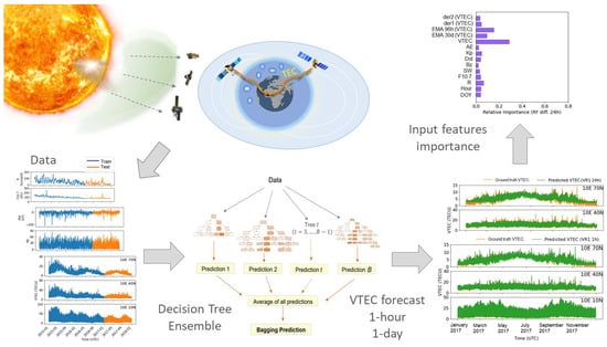
• The relative contribution of the input data to the VTEC forecast is analyzed to provide an insight into what the model has learned, and to what extent our physical understanding of important predictors has increased.

During this study, the following questions were raised:

• Can other, simpler learning algorithms than ANN capture diverse VTEC variations for 1 h and 24 h VTEC forecasts?
• Can ensemble meta-model achieve better performance than a single ensemble member?
• How can VTEC models be improved in terms of data and input features? Also, does the new input dataset bring new information to the VTEC model?
• Can data modification, such as differencing, enhance the VTEC model learning and generalization?

2. Methodology

The VTEC model based on machine learning “learns” directly from the historical data or given examples, which can be understood as past experiences. Learning is achieved by optimizing the performance of a machine learning algorithm for a task of VTEC prediction, which presents the prediction of a continuous variable, commonly referred to as regression in machine learning.

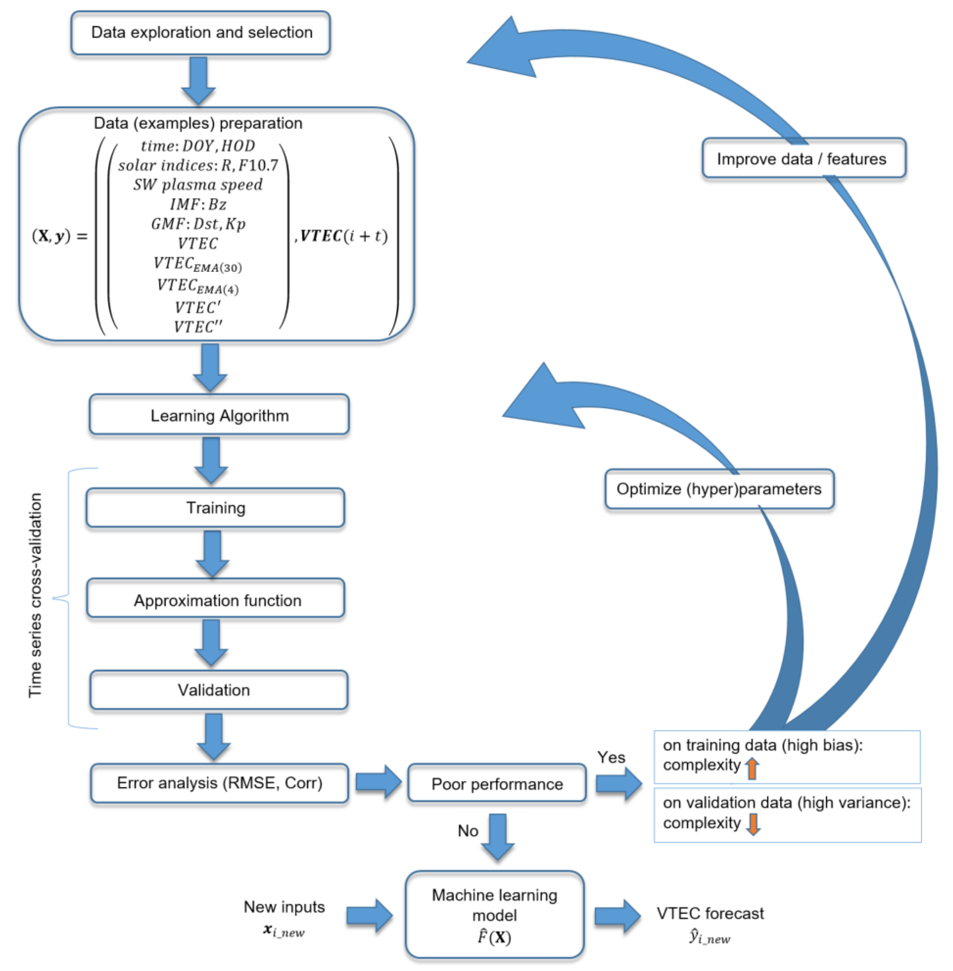
2.1. Data Selection and Preparation

Machine learning is based on data. Therefore, they are impacting the performance of machine learning algorithms to a big extent. Thus, when developing a machine learning model, it is essential to select and prepare data in a way that enables model learning. In addition, the data have to be representative of new cases that may arise in practice in order to generalize well.

In this paper we use supervised learning, where the set of measurements of both input and output data need to be clearly specified and prepared, known as training data, in order to construct the prediction function. Let us define a training sample of vector ${\mathbf{x}}_i$ and an output $y_i=F\left({\mathbf{x}}_i\right)$ at time stamp i with $i=1,2,\dots ,N$ as in Equation (2). Whereas, the vectors ${\mathbf{x}}_i$ can be interpreted as the rows of the $N\times P$ predictor matrix $\mathbf{X}$, the columns represents the input variables ${\tilde{\mathbf{x}}}_p$ with $p=0,1,2,\dots ,P-1$. The components $x_{i,p}$ of the $N\times 1$ column vector ${\tilde{\mathbf{x}}}_p={[x_{1,p},x_{2,p},\cdots ,x_{N,p}]}^T$ represent a time series of the pth input variable. A series of N observations $({\mathbf{x}}_i,y_i)$ was prepared for the training and the cross-validation, from January 2015 to December 2016, while the test dataset covers the period from January 2017 to December 2017. The VTEC values for three grid points at high-latitude (10°, 70°), mid-latitude (10°, 40°), and low-latitude (10°, 10°) were extracted from the Global Ionosphere Maps (GIM) of CODE (Center for Orbit Determination in Europe), while data of solar and magnetic activity were obtained from NASA/GSFC’s OMNIWeb [39]. Therefore, VTEC from GIM CODE was assumed to be the ground truth in this study. Three grid points for VTEC values were selected along the same longitude (10°) in order to represent latitudinal VTEC variations corresponding to different ionosphere regions (low- mid- and high-latitude), alongside other VTEC variabilities. In addition, the hour of the day (HOD) and the day of the year (DOY) were added as input to model the VTEC temporal dependencies. In addition, new input quantities were calculated, such as the exponential moving average (EMA), and first and second time derivatives of VTEC, denoted as VTEC′ and VTEC″. Forecasting is performed for 1 h and 24 h in the future (Equation (2)). Table 1 provides an overview of the data. Separate models were developed for each grid point and each forecast horizon. The dataset for training and cross-validation (January 2015–December 2016) comprises of totally 17,544 examples, while the test dataset (January–December 2017) contains 8760 examples. Datasets were prepared with 1 h temporal resolution.

$$\begin{array}{cc}\hfill & \mathbf{X}=\left[\begin{array}{c}{\mathbf{x}}_1^T\\ {\mathbf{x}}_2^T\\ \cdots \\ {\mathbf{x}}_N^T\end{array}\right]=\left[\begin{array}{c}{x}_{0,1},x_{1,1},\cdots ,x_{P-1,1}\\ x_{0,2},x_{1,2},\cdots ,x_{P-1,2}\\ \cdots \\ x_{0,N},x_{1,N},\cdots ,x_{P-1,N}\end{array}\right]=\left[\begin{array}{c}DO{Y}_1,HO{D}_1,\cdots ,VTE{C}_1^{″}\\ DO{Y}_2,HO{D}_2,\cdots ,VTE{C}_2^{″}\\ \cdots \\ DO{Y}_N,HO{D}_N,\cdots ,VTE{C}_N^{″}\end{array}\right],\hfill \\ \hfill & \mathbf{X}=\left[\begin{array}{c}{\tilde{\mathbf{x}}}_0,{\tilde{\mathbf{x}}}_1,\cdots ,{\tilde{\mathbf{x}}}_{P-1}\end{array}\right],\hfill \\ \hfill & \mathbf{y}=\mathbf{VTEC}(i+t)=\left[\begin{array}{c}{y}_1\\ y_2\\ \cdots \\ y_N\end{array}\right]=\left[\begin{array}{c}{VTEC}_{1+t}\\ {VTEC}_{2+t}\\ \cdots \\ {VTEC}_{N+t}\end{array}\right],\hfill \end{array}$$

(1)

where $t=1$ for the 1 h forecasting and $t=24$ for the 24 h forecasting, for abbreviations see Table 1.

Firstly, the data were preprocessed and prepared with an 1 h time sampling. A few missing values encountered are replaced with the average value of a previous and subsequent value. Some data were not provided as 1 h samples, such as F10.7 and R (24 h samples) and Kp (3 h samples). There, values were interpolated with the previous one, as it is done at the OMNIWeb. Afterwards, two approaches followed:

• After preprocessing, the data $({\mathbf{x}}_i,y_i)$ for $i=1,2,\dots ,N$ are used for the machine learning algorithm. In this paper this dataset is referred as non-differenced data.
• Data (except HOD, DOY, EMA and the time derivatives) are time-differenced $(\Delta {\mathbf{x}}_i,\Delta y_i)$ by calculating the difference between an observation at time $t+24$ h and an observation at time step i, i.e., $\Delta {\mathbf{x}}_i={\mathbf{x}}_{i+24}-{\mathbf{x}}_i$ and $\Delta y_i=y_{i+24}-y_i$. Differencing was used to reduce temporal dependence and trends, as well as, stabilize mean of the dataset [38], by reducing daily variations. In this paper this dataset is referred as differenced data. Values of EMA and time derivatives were calculated from differenced VTEC. At the end, predicted VTEC differences were reconstructed by adding up the VTEC values from the previous day.

2.2. Supervised Learning

Supervised learning can be seen as the function estimation or predictive learning problem. The learning task can be stated as follows: given the values of an input vector ${\mathbf{x}}_i$ (predictor or the independent variable) the aim is to find an approximation $\widehat{F}\left({\mathbf{x}}_i\right)$ of the function $F\left({\mathbf{x}}_i\right)$ which maps the input ${\mathbf{x}}_i$ to the output $y_i$ (response or the dependent variable) and provides a prediction denoted by ${\widehat{y}}_i$ as

$$\begin{array}{cc}\hfill & y_i+e_i={\widehat{y}}_i={\widehat{VTEC}}_{(i+t)}=\widehat{F}\left({\mathbf{x}}_i\right)\hfill \\ \hfill & {\mathbf{x}}_i=[DO{Y}_i,HO{D}_i,R_i,F10.7_i,S{W}_i,B{z}_i,Ds{t}_i,K{p}_i,A{E}_i,\hfill \\ \hfill & VTE{C}_i,VTE{C}_{EMA\left(30\right)}i,VTE{C}_{EMA\left(4\right)}i,VTE{C}_i^{\prime },VTE{C}_i^{″}{]}^T\hfill \end{array}$$

(2)

where $e_i$ is an error. $\widehat{F}(·)$ refers to the approximation function of the nonlinear relationship between the output value of the VTEC forecast and the input vector considering solar, interplanetary and geomagnetic indices, as well as the previous VTEC values. This function is unknown, and is therefore, approximated by optimizing learning algorithms for the task of VTEC forecasting. Using prepared training samples of input and an output in Equation (2), an approximation $\widehat{F}\left({\mathbf{x}}_i\right)$ of the function $F\left({\mathbf{x}}_i\right)$ is estimated by minimizing the value of objective (loss) function L. Employed objective function in this study is the squared error

$$L=\frac{1}{N}\sum _{i=1}^N{e}_i^2=\frac{1}{N}\sum _{i=1}^N{(y_i-{\widehat{y}}_i)}^2.$$

(3)

In this way, the function that describes the input/output relationship is modified as a response to differences between the real VTEC value $y_i$ and generated VTEC prediction ${\widehat{y}}_i$. This represents learning by examples commonly referred as learning or training phase [35].

2.3. Tree-Based Machine Learning Algorithms

Tree-based algorithms are conceptually simple, but powerful machine learning methods that can perform well on both small and large datasets to solve linear and nonlinear modeling problems. Several tree-based machine learning algorithms have been applied in this study, namely Regression tree and ensemble learning such as Random Forest, eXtreme Gradient Boosting (XGBoost), and Adaptive Boosting (AdaBoost).

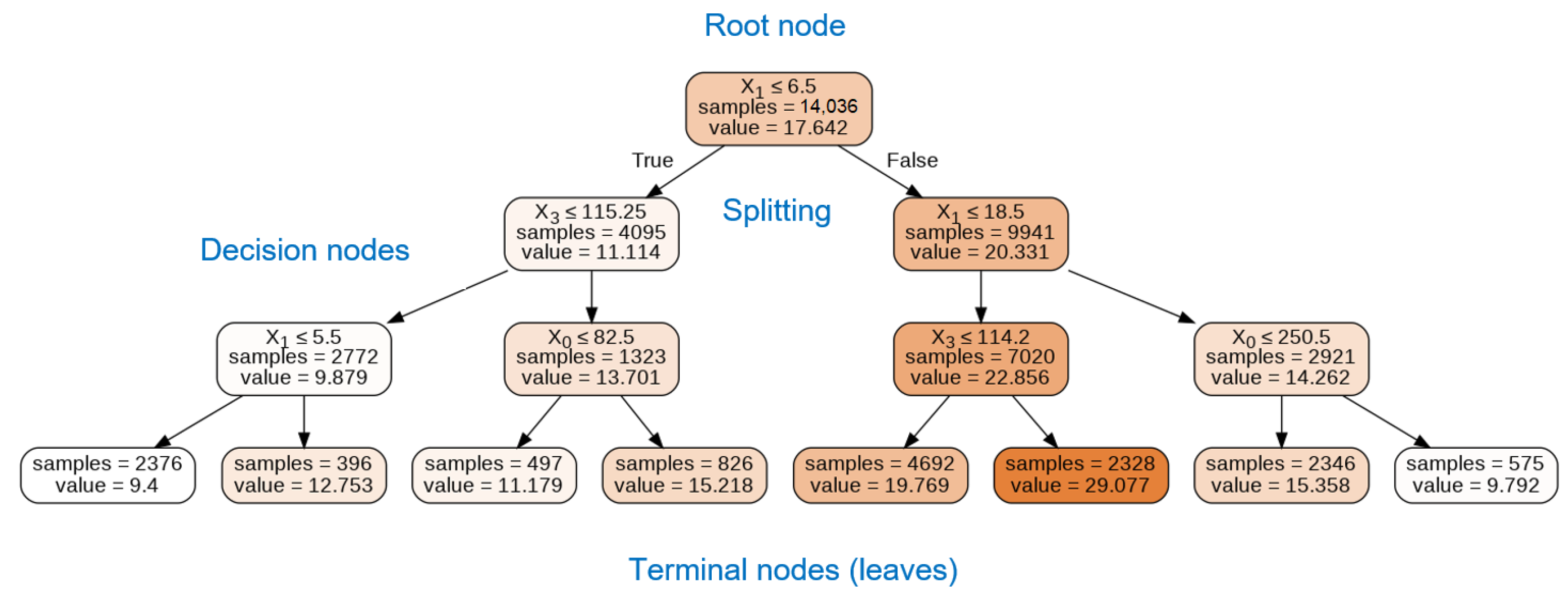
2.3.1. Regression Trees

Decision trees can be classified based on the type of output variable as classification (categorical output) and regression (numerical output) trees. Within this study, the regression tree was grown on the training data using recursive binary splitting. A small regression tree with a depth of 3 is shown in Figure 1 for ease of illustration. There, the tree for VTEC nowcasting was grown using time information, solar and geomagnetic indices as input, and VTEC as output.

Each regression tree model can be formally expressed as

$$T(\mathbf{X};\Theta )=\sum _{j=1}^J{\gamma }_j(\mathbf{X}\in R_j)$$

(4)

with a set of parameters $\Theta ={\{{\gamma }_j,R_j\}}_{j=1}^J$. ${\left\{R_j\right\}}_1^J$ are disjoint regions that collectively cover the space of all joint values of the input variables $\mathbf{X}$ from Equation (4). The regions represent nodes in Figure 1. The parameters of a single tree are the coefficients ${\left\{{\gamma }_j\right\}}_1^J$ and the quantities that define the boundaries of the regions ${\left\{R_j\right\}}_1^J$ such as the splitting variables ${\mathbf{x}}_l$ and the values of those variables (split points) s that splits the nodes of the tree. Since the regions are disjoint, Equation (4) is equal to

$$T\left(\mathbf{X}\right)={\gamma }_j.$$

(5)

The approach begins at the top of the tree, called the root node, as presented in Figure 1. At this point all observations belong to a single region R. The root node in Figure 1 contains 14,036 observation samples. The mean VTEC value $\gamma$ of all observations within the region R is 17.642 TECU. The decision splitting in the rote node is given as ${\tilde{\mathbf{x}}}_1\le 6.5$, which represents the split point, while input variable ${\tilde{\mathbf{x}}}_1$, representing HOD, is splitting variable of the region R. The input space is then divided into two distinct and non-overlapping regions $R_1$ (where the condition is True, i.e., ${\tilde{\mathbf{x}}}_1\le 6.5$) and $R_2$ (where condition is False, i.e., ${\tilde{\mathbf{x}}}_1>6.5$). Therefore, considering a splitting variable ${\tilde{\mathbf{x}}}_p$ with $p=1,2,\cdots ,P-1$ and split point s, two splitting regions can be defined, based on a decision splitting, as [35]

$$\begin{array}{c}\hfill R_1(p,s)=\left\{\mathbf{X}\mid {\tilde{\mathbf{x}}}_p\le s\right\},R_2(p,s)=\left\{\mathbf{X}\mid {\tilde{\mathbf{x}}}_p>s\right\}.\end{array}$$

(6)

The splitting variable $\left({\tilde{\mathbf{x}}}_p\right)$ and split point s are found in a way to solve [35]

$$\underset{l,s}{min}[\underset{{\gamma }_1}{min}\sum _{{\mathbf{x}}_{p,i}\in R_1(p,s)}{(y_i-{\gamma }_i)}^2+\underset{{\gamma }_2}{min}\sum _{{\mathbf{x}}_{p,i}\in R_2(p,s)}{(y_i-{\gamma }_i)}^2]$$

(7)

for any choice ${\mathbf{x}}_l$ and s, the inner minimization is solved by

$${\gamma }_1=\frac{1}{N}\sum _{{\mathbf{x}}_i\in R_1(p,s)}{y}_i,{\gamma }_2=\frac{1}{N}\sum _{{\mathbf{x}}_i\in R_2(p,s)}{y}_i.$$

(8)

The procedure continues further down on the tree, so that the input space, which covers all joint values of the predictor variable $\mathbf{X}$, is divided into J distinct and non-overlapping regions $R_1$,$R_2$, …, $R_J$. This means that the space of the input variables is successively split, i.e., a node is divided into two sub-nodes or regions further down on the tree. A sub-node that is divided into further sub-nodes is called a decision node. The values in each of rectangle (Figure 1) represent the mean VTEC output ${\gamma }_j$ of the $y_i$ falling into region $R_j$ as in Equation (8). A tree stops growing when a node has fewer than a minimum number of observations needed for splitting. This node represents the terminal node or leaf. As can be seen, a decision tree is a simple and highly interpretable method, easily visualized by a two-dimensional graphic, representing an example of a white-box model.

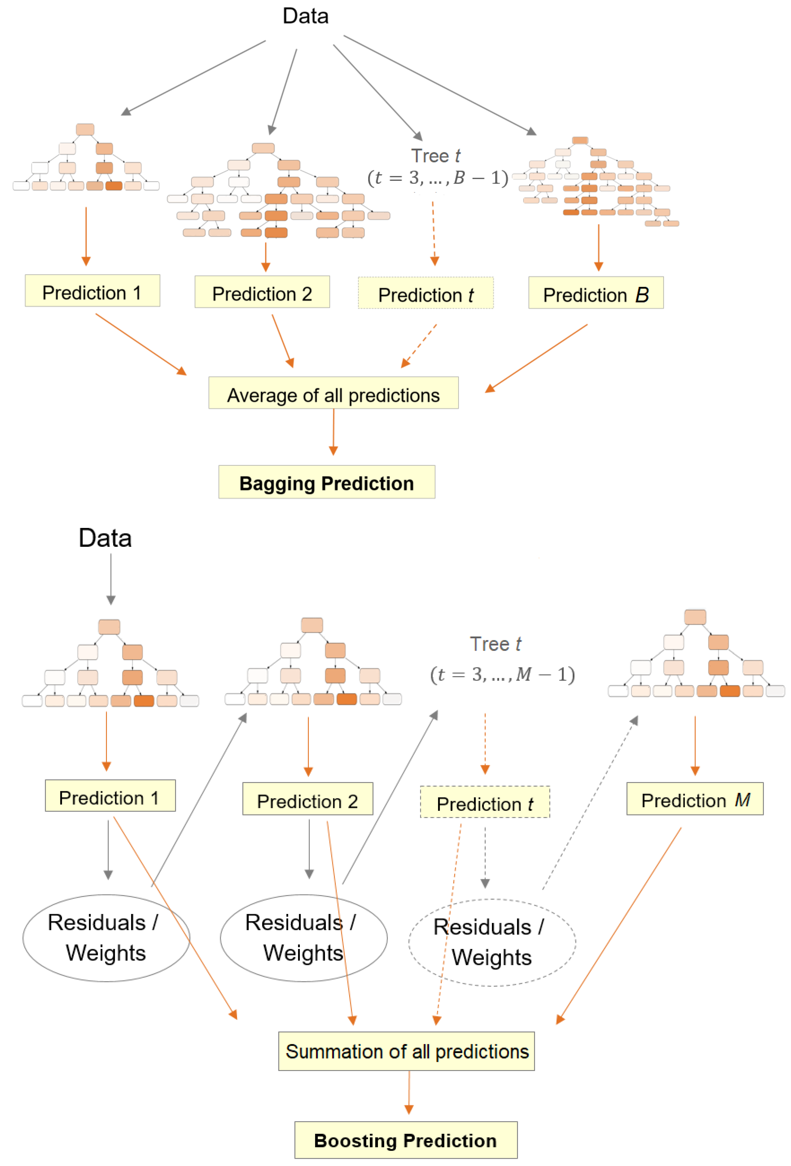
2.3.2. Ensemble Learning

The goal of ensemble learning is to combine predictions of several simple models or base learners, such as an J-node regression tree, to improve generalizability and robustness over a single model. Popular ensemble methods include bagging and boosting.

Random Forest [40] represents a modification of the so-called bagging or bootstrap aggregation technique, which builds a large collection of de-correlated trees and then averages them (Figure 2). When building each tree, a random sample of v input variables is considered as split candidates from a full set of p inputs. Since the forecasting of time series is performed, each new training set is drawn without replacement from the original training set. Thus, a single regression tree $T_b$ (for $b=1,2,\cdots ,B$) is grown by recursively repeating the following steps for each tree node until the minimum node size is reached:

• Select random sample of v input variables from the full set of p variables;
• Find the best splitting variable and split point among the v input variables;
• Split the node into two sub-nodes.

This procedure is applied to all B trees. The function can be expressed as an average of all B trees

$$\widehat{F}\left({\mathbf{x}}_i\right)=\frac{1}{B}\sum _{b=1}^{B}T({\mathbf{x}}_i;{\Theta }_b),$$

(9)

where ${\Theta }_b$ characterizes the bth tree in terms of splitting variables, cutpoints at each splitting node and terminal node values. Breiman [40] demonstrated that randomness and diversity in trees construction lead to lower generalization error and an overall better model with reduced variance.

In the boosting method, the trees are grown sequentially using the information from previously grown trees with modified version of the training data (Figure 2). Each boosted tree can be expressed as

$$F_m\left({\mathbf{x}}_i\right)=F_{m-1}\left({\mathbf{x}}_i\right)+\sum _{y=1}^{J_m}{\gamma }_{jm}({\mathbf{x}}_i\in R_{jm}),$$

(10)

while the final model can be represented as a sum of such trees

$$\widehat{F}\left({\mathbf{x}}_i\right)=F_M\left({\mathbf{x}}_i\right)=\sum _{m=1}^{M}T({\mathbf{x}}_i;{\Theta }_m)=F_{M-1}\left({\mathbf{x}}_i\right)+\sum _{y=1}^{J_M}{\gamma }_{jM}({\mathbf{x}}_i\in R_{jM})$$

(11)

for the set of regions and constants ${\Theta }_m={\{R_{jm},{\gamma }_{jm}\}}_1^{J_m}$. $F_{m-1}\left({\mathbf{x}}_i\right)$ represents the previous model, while left side of Equation (11) represents the current tree.

In the AdaBoost [41], the data are modified by applying weights $w_1,w_2,\cdots ,w_N$ to each of the training examples $({\mathbf{x}}_i,y_i)$ (Figure 2). In the first step, all weights are initialized to $w_i=\frac{1}{N}$, i.e., the data are trained in the usual manner. For each successive step $m=2,3,\cdots ,M$, weights are modified individually and the training is repeated using the weighted observations. More specifically, at step m, the weights increase for the wrongly predicted observations in the previous step, while the weights for correctly predicted observations decrease. Therefore, observations that are difficult to predict receive increasing attention as iterations proceed. In the end, weighted predictions from all trees, i.e., steps, are combined to produce the final prediction as in Equation (11).

Gradient boosting offers a generalization of boosting to an arbitrary differentiable objective function in Equation (3). In the first step, a tree is trained on the original training data. Then for $i=1,2,\cdots ,N$ the gradient is computed as [35]

$$-g_{im}=-\left[\frac{\partial L}{\partial F({\mathbf{x}}_i)}\right]{}_{F=F_{m-1}}.$$

(12)

For the squared error loss, the negative gradient represents the residual between the original and the estimated output $-g_{im}=y_i-F_{m-1}\left({\mathbf{x}}_i\right)$. For each successive iteration ($m=2,\cdots ,M$), a regression tree is fitted to the residuals $g_{im}$ (from the previous iteration) within terminal regions $R_{jm}$ ($j=1,2,\cdots ,J_m$) (Figure 2). Afterwards, the function is updated as in Equation (10). XGBoost [42] is an optimized gradient boosting algorithm that applies shrinkage technique as the regularization strategy to avoid overfitting. This is implemented by scaling the contribution of each tree by a factor $0\le \nu <1$ in Equation (10) as

$$F_m\left({\mathbf{x}}_i\right)=F_{m-1}\left({\mathbf{x}}_i\right)+\nu ·\sum _{y=1}^{J_m}{\gamma }_{jm}({\mathbf{x}}_i\in R_{jm}),$$

(13)

where the parameter $\nu$ represents the learning rate of the boosting procedure.

Voting Regressor is an ensemble meta-estimator that comprises several machine learning models and averages their individual predictions across all models to form a final prediction. This method is useful for a set of well performing models to compensate for their individual weaknesses in order to build a single model that can better generalize.

It is often useful to provide information about the underlying relationships between the inputs and the outputs of the model to improve understanding of what the model has learned. Using tree-based methods, it is possible to easily estimate the relative importance or contribution of each input variable to forecasted VTEC. Proposed by [43], it is calculated as the improvement in minimization of the objective function as a result of using input variable ${\mathbf{x}}_l$ to split the node within a tree. The relative importance of a variable ${\mathbf{x}}_l$ is then calculated as the sum of such improvements overall all internal nodes, for which it was chosen as the splitting variable. For a collection of decision trees ${\left\{T_m\right\}}_1^M$, the relative importance is averaged over all trees.

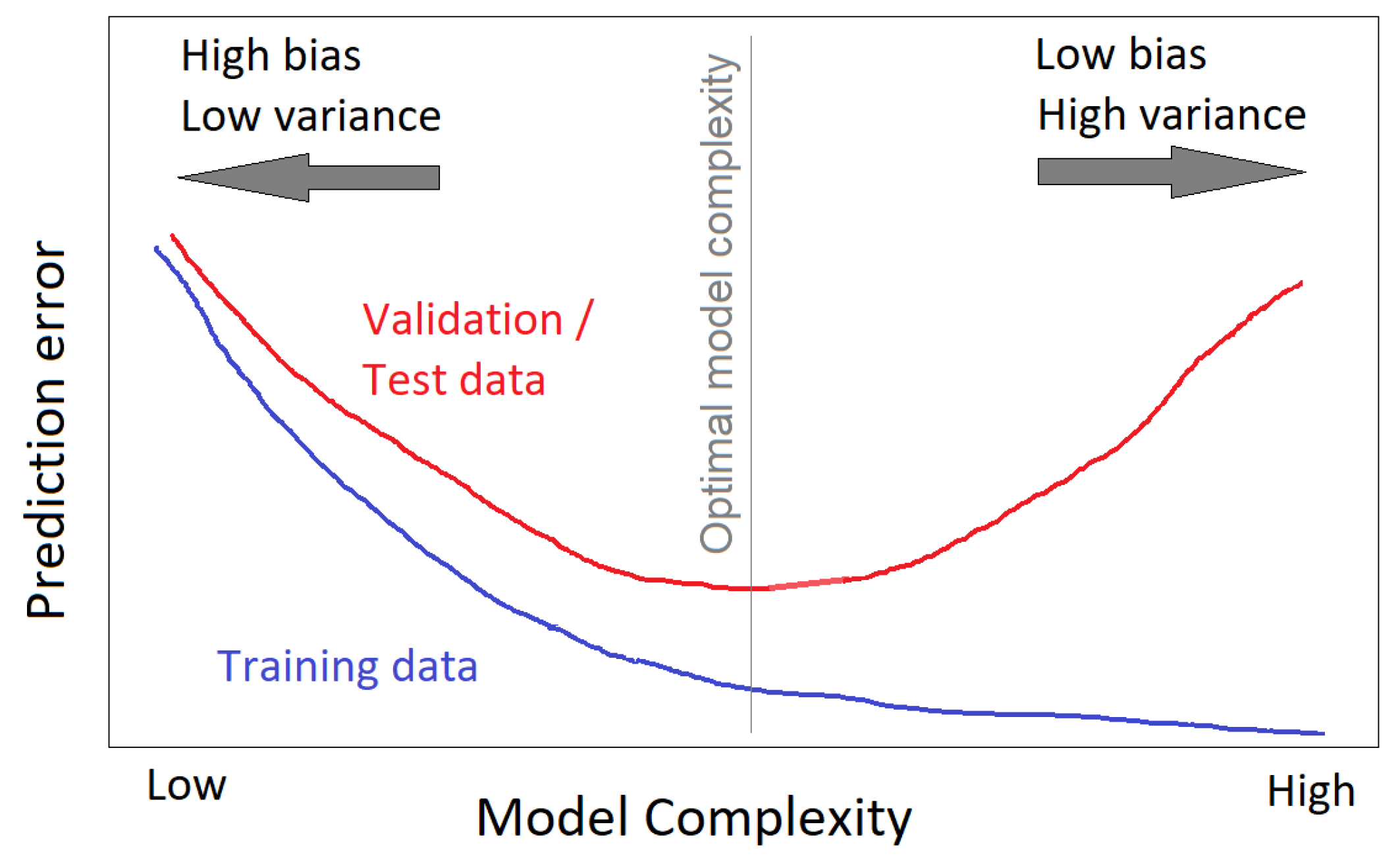
2.4. Model Selection and Validation

Parameters, such as the splitting variable and the value of the splitting point, are estimated from data during the learning phase using an optimization algorithm, as already discussed. However, every learning algorithm has certain parameters, known as hyperparameters, that cannot be estimated from data, but need to be tuned for a given modeling problem. Hyperparameters determine the model architecture and control the model complexity. Their optimal values depend on the data and the problem. They are typically found by trying different combinations and evaluating the performance of each model. However, the residual sum of squares on the training data cannot be used to determine their values, since that would reduce the ability of a model to generalize future data. Therefore, we used three sets of data, namely the training set (to train the model), validation (to measure the model performance and optimize its parameters/hyperparameters), and test set (used only at the end to estimate the generalization error). In this way, we selected the most optimal (hyper)parameters and provided a measure of the overall reliability and accuracy of the proposed machine learning models.

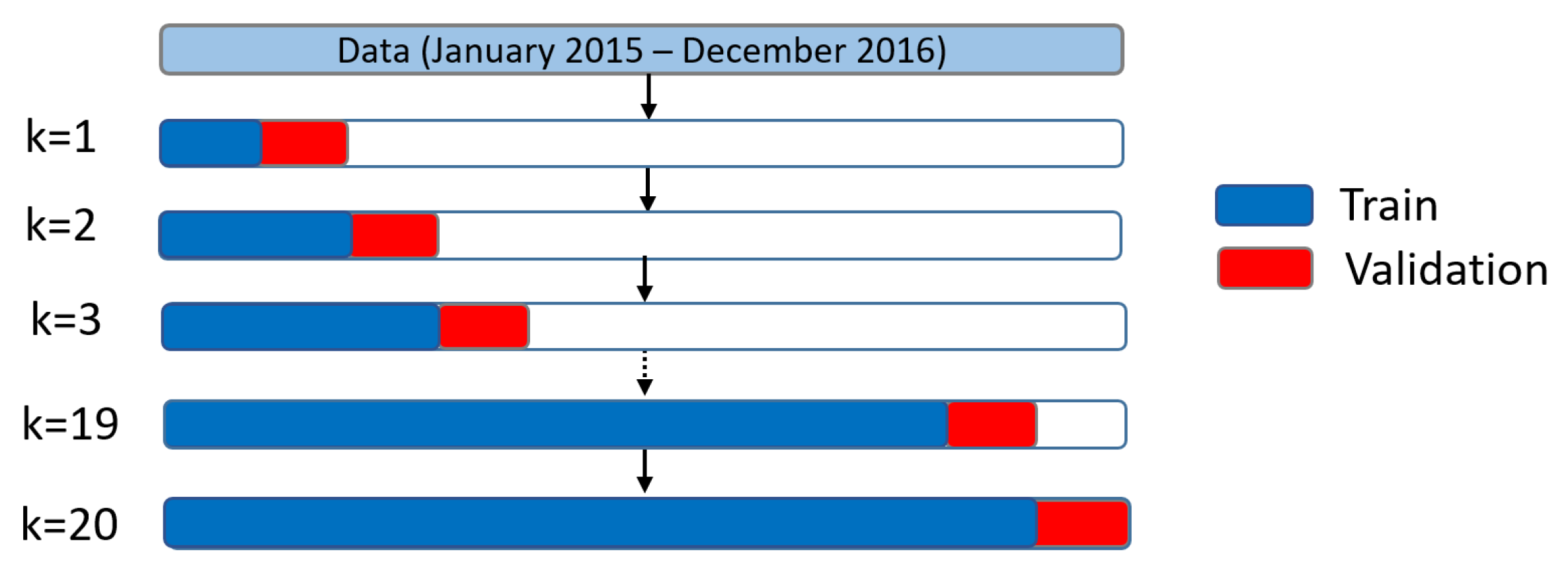
2.4.1. Time Series Cross-Validation

Since observations are temporally dependent, we applied the time series cross-validation technique to preserve a temporal dependency, where a model is trained, optimized, and evaluated on a rolling basis using many data folds. For reliable performance evaluation, a large number of folds should be adopted [44]. The data are divided into two folds at each iteration: a training set and cross-validation set (Figure 3). The model is trained on the training set, while the (hyper)parameters, that minimize the RMSE, are found using the cross-validation set. The training set consists only of observations that occurred prior to observations that form the cross-validation set. The cross-validation data from the previous iteration are included as part of the next training data set and subsequent data points are forecasted. The final metric is calculated as the average of the RMSE obtained in each cross-validation iteration.

2.4.2. Model Architecture

Hyperparameters of tree-based models, that commonly need to be optimized, are the maximum depth of the tree (max_depth), number of trees in ensemble learning (n_estimators), the value of learning rate (in boosting), etc. The size of a tree controls the complexity of the model. Too large tree results in a more complex model that can overfit the training data, and consequently may not generalize well. The size $v=6$ (max_features) of the random subsets of input variables is considered when splitting a node to introduce randomness in tree construction in order to improve the accuracy and reduce the overfitting problem. The lower size of v reduces the correlation between any pairs of trees in Random Forest and hence, reduces overfitting. However, if there are only a few relevant variables out of many, v should be set to a higher value, so that the algorithm can find the relevant variables. For XGBoost, smaller values of learning rate $\nu$ (more shrinkage) result in a lower test error but require a larger number of iterations m [45]. Moreover, data are subsampled for every tree to further prevent overfitting. Optimal hyperparameters and the range of values used to search optimal values for hyperparameters are provided in

Table 2. Hyperparameters of developed machine learning models.

Model	Selected Hyperparameters	Range of Search
	max_depth = 5–8	[4, 5, 6, 7, 8, 9, 10, 15, 20]
Decision Tree	min_samples_split = 10–20	[2, 5, 10, 15, 20]
	min_samples_leaf = 10	[2, 5, 10, 15, 20]
	max_features = 6	[4, 5, 6, 7, 8]
	max_depth = 8–10	[4, 6, 8, 10, 12, 15, 20]
Random Forest	min_samples_split = 10	[2, 5, 10, 15, 20]
	min_samples_leaf = 5	[2, 5, 10, 15, 20]
	n_estimators = 300	[50–500] interval of 50
AdaBoost	max_depth = 6–8	[3, 4, 5, 6, 7, 8, 9, 10, 15]
	n_estimators = 50	[50, 100, 150, 200, 300]
	max_depth = 4–6	[3, 4, 5, 6, 7, 8, 9, 10, 15]
XGBoost	n_estimators = 100	[50, 100, 150, 200, 300]
	learning_rate = $0.1$	[0.01, 0.05, 0.1, 0.15, 0.2, 0.25, 0.3]
	subsample = $0.5$	[0.3, 0.5, 0.7, 1]

, where min_samples_split and min_samples_leaf are the minimum number of samples required in an internal node and leaf node, respectively. Similar values for hyperparameters were found for the global XGBoost VTEC model in [29], namely 100 trees, a maximum tree depth of 6, and a learning rate of 0.1.

Individual models were trained for each grid point and each forecast window, i.e., six models were developed for each machine learning method in

Table 3. Overview of developed VTEC machine learning models.

Abbreviation	Machine Learning Model	Approach
DT	Decision (Regression) Tree	Single tree
RF	Random Forest	Bagging ensemble
AB	AdaBoost	Boosting ensemble
XGB	XGBoost	Boosting ensemble
VR1	Random Forest, AdaBoost & XGBoost	Meta-ensemble
VR2	Random Forest & XGBoost	Meta-ensemble

. A total of 72 models were developed: 36 for non-differenced data and 36 for differenced data. Learning algorithms were implemented in the Python programming language using Scikit-learn library [46].

Figure 4 depicts a flowchart of the VTEC machine learning model development. Based on its performance on training and validation data, the model was optimized in terms of hyperparameters and data. In the case of high bias, the model with an approximation function is not complex enough, and therefore, it underfits the data. As the model complexity increases, the variance tends to increase, while the bias tends to decrease, which results in a decrease in training error (Figure 5). However, too much complexity leads to an increase in the validation error and consequently to a large test error due to overfitting (high variance). The aim is to find a balanced model that neither learns from the noise (data overfitting) nor makes poor assumptions about the data (data underfitting). The final model complexity is chosen in a way to trade off bias with variance, i.e., balance bias with variance to minimize the validation error and, consequently, the test (generalization) error. High bias was fixed by adding new input features and increasing the values for max_depth, max_features, n_estimators. The high variance was addressed by decreasing the values for max_depth, max_features, n_estimators, learning_rate, subsample, as well as increasing the values for min_samples_split and min_samples_leaf (Table 2).

The training and validation time with 20-folds for the single Decision Tree model is under 5 s, while it increases for the ensemble learning models from 30 s for XGBoost to about 5 min for Random Forest (

Table 4. Execution time in seconds of the VTEC models using NVIDIA Tesla P100 GPU with 16 GB memory.

Machine Learning Model	Training and Validation (s)	Testing (s)
DT	2–4	<0.01
RF	300–330	∼0.30
AB	65–85	∼0.10
XGB	30–40	∼0.05
VR1	∼250	∼0.35
VR2	∼200	∼0.25

). Overall, their execution time is under 5 min, while the testing time is less than one second for each of the models, demonstrating the computational efficiency of the proposed models.

3. Results

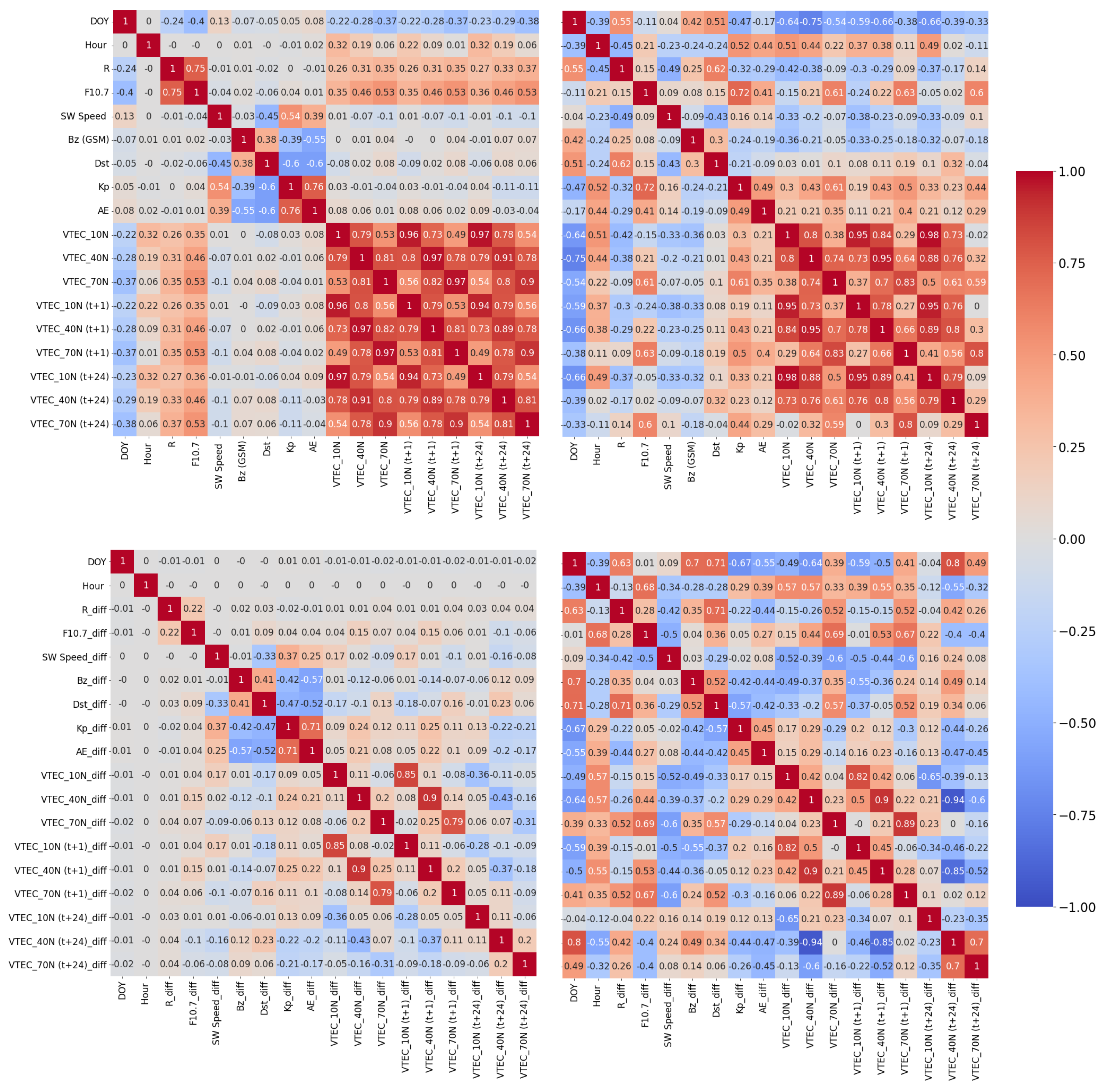
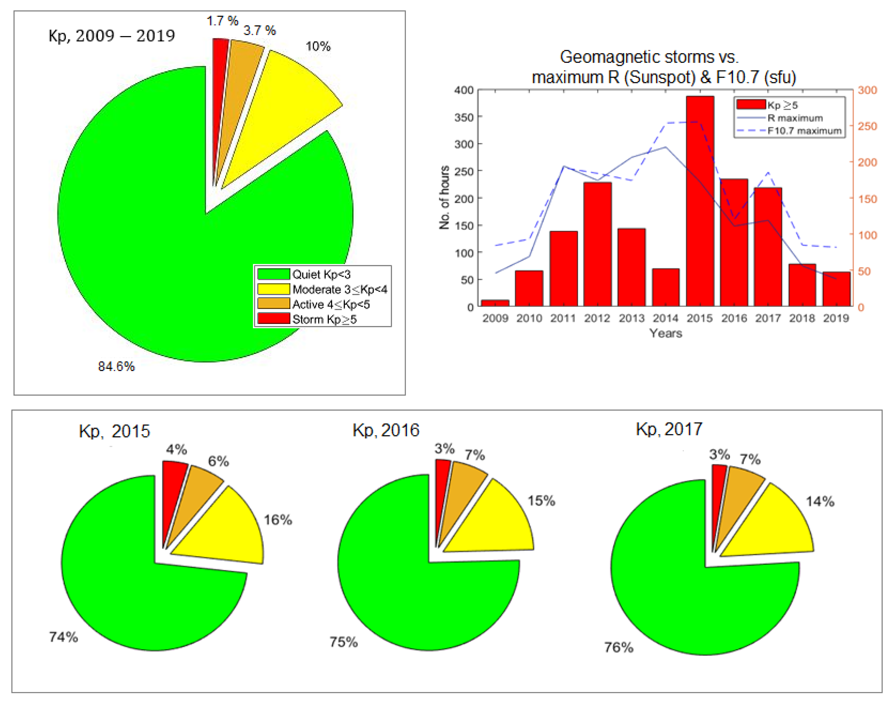
3.1. Exploratory Data Analysis

Exploratory data analysis is performed to identify significant patterns and correlated data, as well as to summarize their properties to support the selection of input data for the machine learning model. It is important to prepare a suitable dataset for learning algorithms to enable the learning of important features for VTEC forecasting. Our goal was to create training data with enough relevant and not too many irrelevant inputs and also not too much correlated input data. These properties can be verified with the correlation matrix between the input and the output data (Figure 6).

Using the non-differenced data (Figure 6, top left), a weak positive and negative linear relationship between VTEC and the time information, hour and DOY, respectively, can be noticed. A weak to a moderate positive relationship can be seen between VTEC and solar indices (R and F10.7). The relationship to the solar wind and magnetic activity data (Bz, Dst, AE) indicates a very weak to no relationship at all. On the other hand, the relationship between differenced VTEC and the time information disappears and there is a very weak relationship with solar indices (Figure 6, bottom left). However, the relationship between differenced VTEC and differenced data of solar wind and magnetic activity increased. The relationship between VTEC(t) with VTEC(t + 1 h) and VTEC(t + 24 h) is very high positive for non-differenced data, while for differenced data is high positive for VTEC(t + 1 h) and low positive for VTEC(t + 24 h). The heatmap for periods of strong and severe geomagnetic storms (Kp ≥ 7) reveals a weak to moderate relationship between VTEC and all input data (Figure 6, right). The relationship to data of solar wind speed, Bz, Kp, and AE is significantly increased. These relationships are not visible in the heatmap over the entire training period (Figure 6, left) as these events are rare and unrepresented in the dataset (Figure 7). However, during the space weather event, it becomes apparent that these data are relevant and should be taken into account. The VTEC prediction during space weather events is clearly a case of unrepresented classes, i.e., data imbalance, where space weather events are in minority compared to the quiet period.

As highlighted in Figure 7 (top left), $85\%$ of the 3 h Kp data from 2009 to 2019 indicates quiet conditions in the geomagnetic field, while only $2\%$ of the Kp data have reached an index of 5 or higher. This indicates that geomagnetic storms are strongly underrepresented and occur rather rarely, leading to imbalanced examples. On the other hand, these examples are of special interest as they contain useful knowledge and important information for forecasting purposes. Machine learning boosting algorithms have been shown to be suitable for applications with imbalanced data [47]. The number of geomagnetic storm conditions (Kp $\ge 5$) was the highest in the years after the solar maximum (reached in April 2014), i.e., from 2015 to 2017, and in 2012, before the solar maximum (Figure 7, top right). Years 2015 and 2016 have more of these events than other years (Figure 7, bottom). In addition, they are near the solar maximum. Therefore, they have been chosen for training and cross-validating the models to have more examples of storm events and near-solar maximum conditions. The subsequent year 2017 is selected for testing as it includes the strongest storm of solar cycle 24 (in September 2017). In the training dataset, there are 99 days with reported Kp $\ge 5$, with 56 days in 2015 and 43 days in 2016. In the test dataset, Kp $\ge 5$ applies for 37 days.

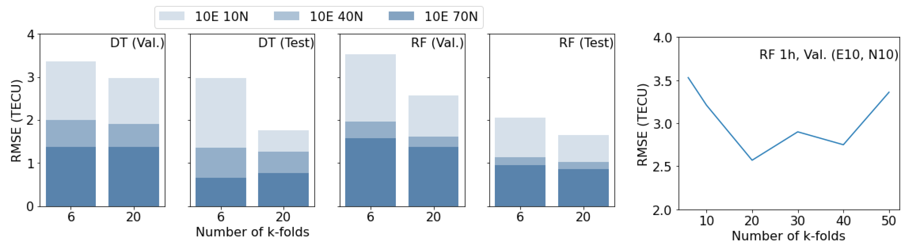
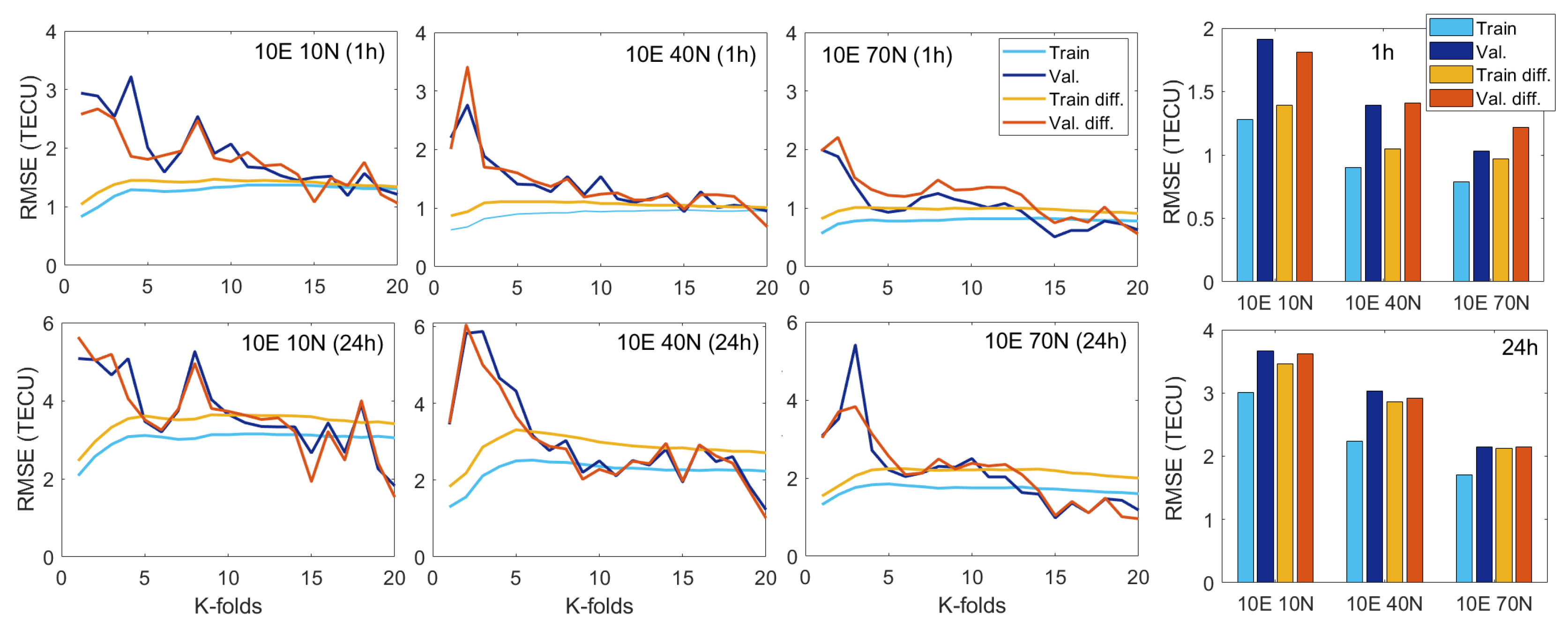
3.2. K-Fold Selection for Cross-Validation

To achieve optimal results, the appropriate k-fold size was analyzed with respect to the accuracy of two machine learning models, namely Decision Tree and Random Forest. For the analysis VTEC is predicted for high-latitude, mid-latitude and low-latitude ionospheric regions using the varying k-fold sizes: $k=(6,10,20,30,40,50)$ (Figure 8). The graph to the left presents the RMSE for cross-validation and test datasets with Decision Tree and Random Forest for 6 and 20 folds. The low-latitude VTEC forecast (RMSE) is improved for about 1 TECU by increasing the k-fold size from 6 to 20, while the RMSE for the high and mid-latitude VTEC is similar for both k-folds. Only for Decision Tree, a slight RMSE degradation for the high-latitude VTEC is observed for test data with 20 folds, which may be due to overfitting as a single tree tends to overfit the data. However, the improvement in the low-latitude VTEC is significantly higher. The graph to the right illustrates the RMSE as a function of the number of k-folds for the low-latitude VTEC, where $k=20$ folds appear to be optimal. The low-latitude VTEC has more complex variations, such as those due to the equatorial anomaly. Using a smaller k-fold size, the model is trained and cross-validated with larger data samples in a single k-fold with a smaller number of iterations. In that case, it may overlook some VTEC variations that are not much represented in the single split. By increasing the k-folds size, the model is trained on smaller data subsets with more iterations. Thus, the signal can be learned better. However, too large k-fold will result in very small data subsets that can lead to overfitting during training, resulting in higher RMSE on the cross-validation set, as for $k=50$. Similar behavior is observed for the boosting models. However, the goal is to neither overfit nor underfit the data. From Figure 8 it is apparent that $k=20$ folds are optimal for a 2-year cross-validation period (2015–2016).

RMSE on training and cross-validation data sets is presented for each k-fold for the model VR1 in Figure 9. Training curves are mostly constant after the 5th fold, while cross-validation curves are changing more significantly. The training set is small in the first folds, which results in lower RMSE during training, as it is easier to fit the smaller dataset. On the other hand, the larger RMSE values are for cross-validation, as such a small training data set is not representative. While increasing the number of k-folds, the training data set becomes larger, which slightly increases RMSE during training, while decreasing RMSE during cross-validation. Thus, the largest errors for the cross-validation are mostly in the first 5 folds. After the 10th fold, RMSE values of cross-validation are similar to RMSE values of training or even smaller as k further increases. The average RMSE values for training and cross-validation for all k-folds are summarized in the bar graphs in Figure 9. Differences in RMSE between training and cross-validation are larger for non-differenced data than for differenced data. Differenced data have a lower training RMSE, while the cross-validation RMSE is mostly similar between differenced and non-differenced data.

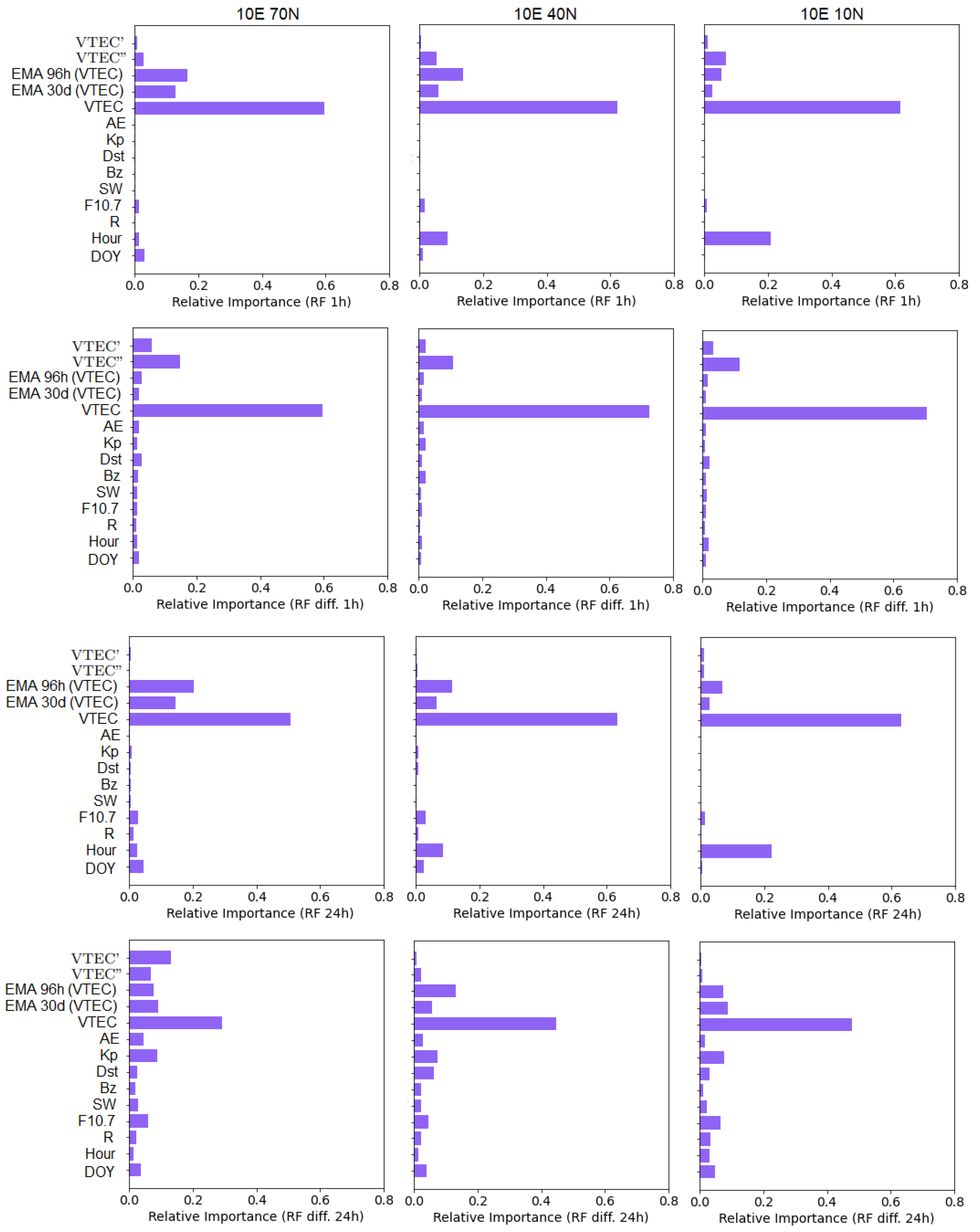
3.3. Relative Importance of Input Variables to VTEC Forecast

Relative importance of the input variables for the 1 h and 24 h VTEC forecasts using non-differenced and differenced data for the period 2015 - 2016 is estimated (Figure 10), including an analysis for geomagnetic activity conditions (Kp $\ge 5$) (Figure 11).

The results demonstrate that the previous VTEC information as an input variable has the largest contribution to the VTEC prediction. Its significance for non-differenced data is about $60\%$, while for differenced data it is from $60\%$ to $70\%$ for 1 h and $30\%$ to $50\%$ for 24 h forecasts (Figure 10). Another important input variables for non-differenced data are exponential moving averages, especially over the last four days (96 h). On the other hand, time-derivatives of VTEC are more important for 1 h forecast with differenced data, in particular the first derivative. For 24 h forecast with differenced data, exponential moving averages have higher importance. For the high-latitude ionospheric region (10°70°), the second derivative has also a higher contribution. For models with non-differenced data, other dominant input variables are temporal information (hour and DOY), followed by solar activity data (F10.7 index), while other variables (solar wind and magnetic field) have little or no influence on the VTEC forecast. In the case of differenced data, on the other hand, the contribution of the temporal information decreased. At the same time, the contribution of other input variables increased, namely solar wind speed (SW) and indices of magnetic field (AE, Kp, Dst, Bz). Their significance is larger for 24 h forecasts.

During geomagnetic storm conditions, the relative importance of input variables, describing the solar activity, solar wind, and magnetic activity, increased for almost all ionospheric regions, especially for non-differenced data, while the contribution of previous VTEC value mostly decreased (Figure 11). In addition, the contribution of the first time derivative for non-differenced data increased. It is especially interesting to see the higher significance of the AE index for high-latitude, the Kp index for mid-latitude, and the Dst index for low-latitude ionospheric regions for differenced data, having in mind that these indices are measured in those regions.

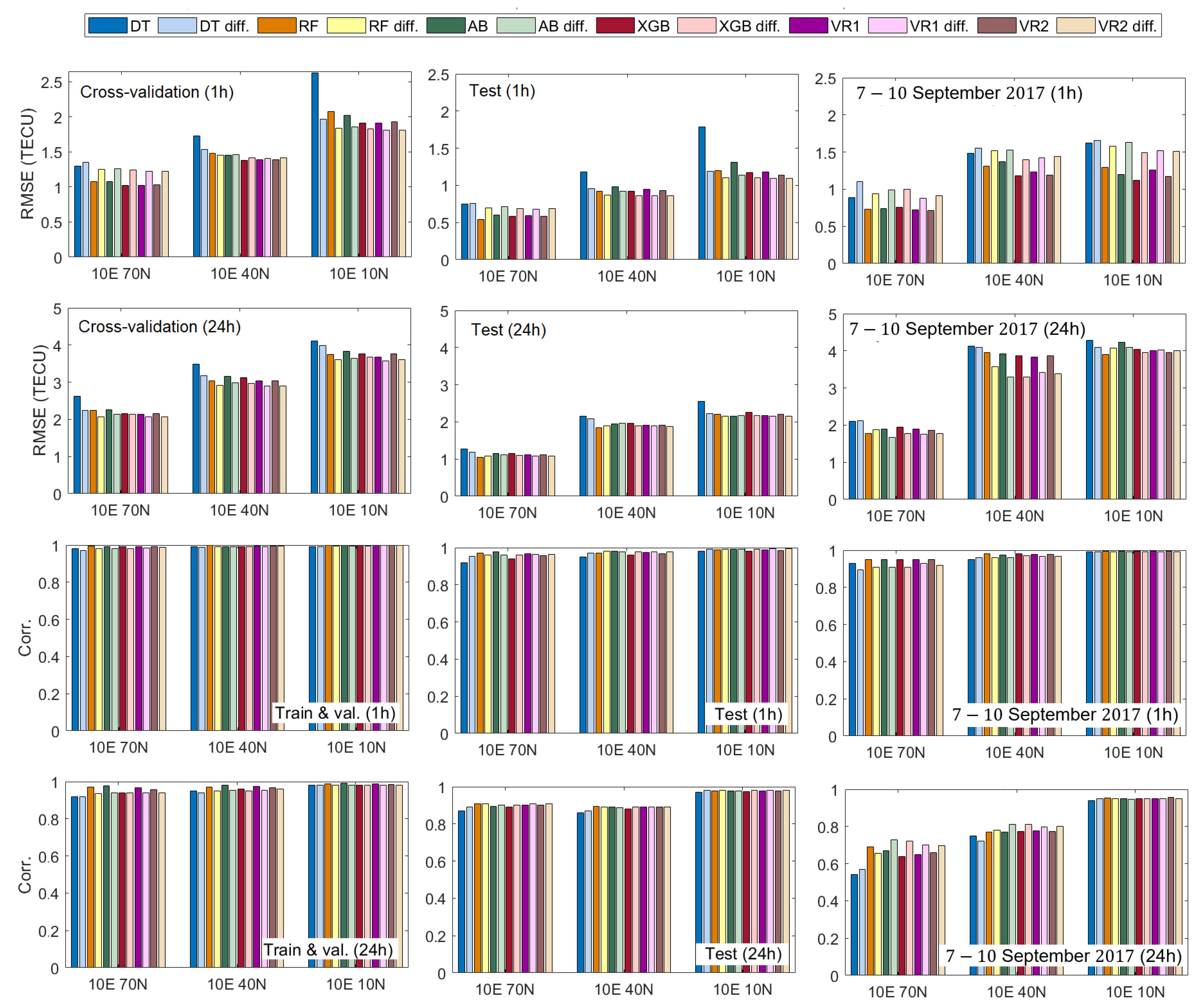
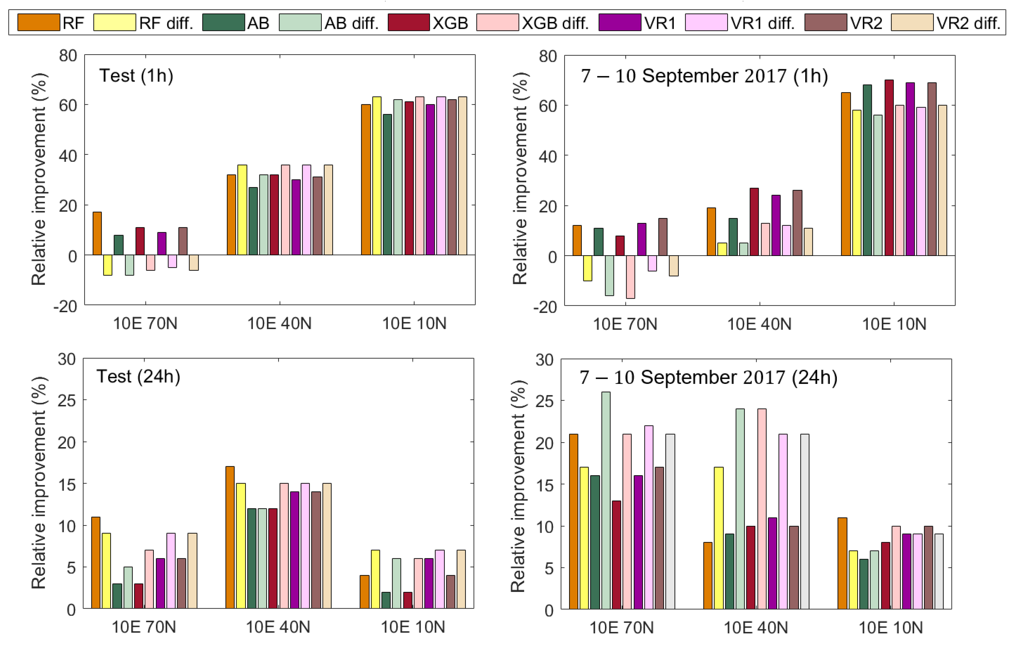
3.4. Accuracy Performance of Machine Learning Models

The RMSE and correlation coefficients for cross-validation, test, and geomagnetic storm (7–10 September 2017) datasets for the 1 h and 24 h forecasts with different machine learning models, namely Decision Tree and ensemble learning (Random Forest, AdaBoost, XGBoost and Voting Regressors), using two types of data (non-differenced and differenced) are presented in Figure 12. The period of the severe geomagnetic storm (7–10 September 2017) covers the main and recovery phase of the storm. In addition, an overview of the RMSE for the year 2017 and for the storm in September 2017 is shown in

Table 5. Overview of RMSE for different machine learning models for test period of year 2017 and severe geomagnetic storm 7–10 September, 2017 for high-latitude (10E 70N), mid-latitude (10E 40N) and low-latitude (10E 10N) VTEC. The subscript diff. indicates models trained on differenced data. The maximum and minimum values of the RMSE are marked in red and green, respectively.

	DT	RF	AB	XGB	VR1	VR2
	70N, 40N, 10N	70N, 40N, 10N	70N, 40N, 10N	70N, 40N, 10N	70N, 40N, 10N	70N, 40N, 10N
2017	RMSE (TECU)	RMSE (TECU)	RMSE (TECU)	RMSE (TECU)	RMSE (TECU)	RMSE (TECU)
1 h	0.75, 1.18, 1.79	0.54, 0.92, 1.20	0.60, 0.98, 1.31	0.59, 0.92, 1.17	0.59, 0.95, 1.18	0.58, 0.93, 1.14
1 hdiff.	0.76, 0.96, 1.19	0.70, 0.87, 1.10	0.71, 0.92, 1.14	0.69, 0.86, 1.10	0.68, 0.86, 1.09	0.69, 0.86, 1.09
24 h	1.28, 2.15, 2.55	1.06, 1.86, 2.20	1.15, 1.95, 2.26	1.15, 1.96, 2.25	1.11, 1.91, 2.17	1.11, 1.92, 2.21
24 hdiff.	1.18, 2.08, 2.22	1.08, 1.89, 2.15	1.12, 1.96, 2.17	1.10, 1.89, 2.17	1.08, 1.89, 2.15	1.08, 1.88, 2.15
7–10 September
1 h	0.89, 1.48, 1.62	0.73, 1.31, 1.29	0.74, 1.37, 1.20	0.76, 1.18, 1.12	0.72, 1.23, 1.16	0.71, 1.19, 1.17
1 hdiff.	1.10, 1.55, 1.66	0.94, 1.52, 1.58	0.99, 1.53, 1.63	1.00, 1.40, 1.49	0.88, 1.42, 1.52	0.91, 1.44, 1.51
24 h	2.10, 4.12, 4.29	1.77, 3.95, 3.95	1.89, 3.92, 4.23	1.95, 3.87, 4.04	1.90, 3.84, 4.01	1.86, 3.87, 3.96
24 hdiff.	2.12, 4.09, 4.10	1.87, 3.57, 4.08	1.67, 3.29, 4.09	1.77, 3.29, 3.96	1.76, 3.41, 4.02	1.78, 3.39, 4.00

.

The RMSE for the cross-validation dataset is higher than for the test dataset because the training period (2015–2016) includes larger absolute VTEC values as it is closer to the solar maximum (in April 2014). The RMSE is about twice higher for 1 day forecast than for 1 h forecast for all the models. The VTEC forecast with a single Decision Tree tends to have the highest RMSE and the lowest correlation coefficients for all datasets. Ensemble learning improved the accuracy. The lowest RMSE is mostly achieved with the Random Forest, XGBoost and Voting Regressor models. During the severe geomagnetic storm in September 2017, the RMSE is about 0.3 to 0.5 times higher for the 1 h forecast and 0.7 to 1 times higher for the 24 h forecast than for the entire test year 2017 (Table 5). The boosting method provided the lowest RMSE during the space weather event (XGBoost in particular), demonstrating its usefulness for predicting rare events. From the cross-validation and test results (Figure 12) it can be seen that the lower RMSE for the mid- and low- latitudinal ionospheric regions for 1 h and 24 h forecasts mainly have models trained on differenced data. This can be also observed for the high-latitude ionosphere for the 24 h forecast. The correlation coefficients are above $90\%$ for the 1 h and 24 h forecast horizons for the training and cross-validation dataset (2015–2016), while the correlation coefficients for the test dataset (2017) are above $90\%$ for the 1 h and above $85\%$ for the 24 h forecast horizons. For the year 2017, the lowest RMSE for the high-latitude VTEC is 0.54 TECU and 1.6 TECU for the 1 h forecast (non-differenced data) and the 24 h forecast (differenced data), respectively (Table 5). The lowest RMSE for VTEC in the mid-latitude is 0.86 TECU and 1.86 TECU for the 1 h (differenced data), and the 24 h (non-differenced data) forecast horizons, respectively. The highest accuracy of the VTEC forecast for the low-latitude region is the RMSE of 1.09 TECU and 2.15 TECU for the 1 h and 24 h forecast horizons, respectively, both with differenced data.

On the other hand, during the storm, models trained on non-differenced data have a smaller RMSE and a higher correlation coefficient for the 1 h forecast, while for the 24 h forecast the smallest RMSE and the highest correlation coefficients are mostly for models with differenced data. Correlations between the ground-truth VTEC and predicted VTEC for the storm test period are from $90\%$ for the 1 h forecast, while for the 24 h forecast they are from $55\%$ (the highest $73\%$), $72\%$ (the highest $81\%$) and $94\%$ (the highest $95\%$) for the high-latitude, mid-latitude, and low-latitude ionospheric regions, respectively. For the 1 h forecast, the highest correlation coefficients are achieved with Voting Regressor and non-differenced data, while for the 24 h forecast the highest correlation coefficients are with boosting methods (AdaBoost and XGBoost) and differenced data. The lowest RMSE for the high-latitude VTEC is 0.71 TECU and 1.67 TECU for the 1 h (non-differenced data) and 24 h (differenced data) forecast, respectively (Table 5). In terms of the mid-latitude VTEC, the lowest RMSE is 1.18 TECU and 3.29 TECU for the 1 h (non-differenced data) and 24 h (differenced data) forecast, respectively. The low-latitude VTEC forecast achieved the lowest RMSE of 1.12 TECU and 3.96 TECU for the 1 h (non-differenced data) and 24 h (non-differenced and differenced data) forecast, respectively.

The relative RMSE change with respect to the persistence (naive) forecast is presented in Figure 13. The persistence model considers that the VTEC(i + t) is equal to the VTEC(i), where t takes values of 1 and 24 for the 1 h and 24 h forecasting, respectively, i.e., we assume the state of the frozen ionosphere with respect to the previous hour or previous day. Persistence forecast is the most common baseline method to measure the forecast performance in supervised machine learning, as well as, in data-driven, physics-based and traditional statistical VTEC forecasting [24,31,48,49,50]. The models for the 1 h forecast of the low-latitude VTEC have reduced RMSE of about 60% for the test period and about 70% during the geomagnetic storm with respect to the baseline. The relative RMSE reductions with respect to the persistence forecast are up to 20%, near 40%, and around 60% for the high-, mid-, and low- latitude VTEC points, respectively, for the 1 h forecast with a non-differenced RF model. For the 24 h forecast, the machine learning models have a lower RMSE by 10–25%, 15–25%, and 5–10% for the high-, mid-, and low- latitude VTEC points, respectively. For the 1 h forecast of the high-latitude VTEC, the RMSE is increased when using differenced data. However, in the case of the 24 h forecast, the models with differenced data mostly forecast the high-latitude VTEC by 5% to 10% lower RMSE than the models with non-differenced data. In addition, they improve the 1 h and 24 h mid- and low-latitude VTEC forecasts by about 2–5% with respect to the models with non-differenced data in 2017. For the storm period, models with non-differenced data provide 1 h forecast for the VTEC points at high-, mid-, and low-latitudes with an RMSE of about 10–15% lower than the models with differenced data. On the other hand, for the longer (24-h) forecast, the models with differenced data mostly outperform the models with non-differenced data, especially during the storm, when the relative RMSE decrease is up to 10% for the high-latitude VTEC and 10% to 15% for the mid-latitude VTEC. The differences in the low-latitude 24 h VTEC forecast are smaller (<4%) between different models and data.

Machine learning performance depends highly on data and, therefore, data should be prepared in a way to enhance learning. Figure 14 shows the VR1 model improvement by including the inputs such as exponential moving averages and time derivatives of VTEC. First, models were trained with the first ten input data in Table 1, i.e., without exponential moving averages and time derivatives, denoted as Data1. Later those inputs are added to improve learning, referred to as Data2. For both non-differenced and differenced data, the RMSE is reduced (by 0.2 to 0.5 TECU) as additional inputs of moving averages and time derivatives are added.

Further, differenced and undifferenced data were combined, where exponential moving averages and time derivatives were calculated from non-differenced VTEC, to forecast non-differenced VTEC (Figure 15). The analysis was done for the XGBoost model, because it is fast compared to other models (Table 4), while accuracy is comparable between the models (Table 5). The RMSE for the 1 h VTEC forecast for test data including the severe geomagnetic storm is similar for models with non-differenced data and data combination. For the 24 h forecast, the RMSE for mid- and low-latitude VTEC with data combination is lower than for the non-differenced data, while more similar to the RMSE for differenced data (Figure 15). Data combination for forecasting non-differenced VTEC improved the model accuracy compared to the non-differenced data for the 24 h forecast and during the space weather event.

Values of VTEC from machine learning models and GIM CODE VTEC were analyzed in more detail for the severe space weather event in September 2017 (Figure 16, left) including their differences (Figure 16, right).

The CMEs with earthward trajectories were emitted from the Sun on 4 and 6 September 2017 [51]. The first CME arrived on 6 September at about 23:43 UT leading to moderate geomagnetic conditions on 7 September (Figure 16). The solar wind shock from the second CME, originating from the intense X9.3 solar flare of September 6, caused a sudden storm commencement (SSC) at about 23 UT on 7 September. This led to severe geomagnetic storms in September with the maximum value of Kp = 8. The main phase of the storm was characterized by the two pronounced minima of Disturbance storm time (Dst) index at about 1:00 and 14 UT on 8 September. Afterward, the recovery phase started and lasted for about 3 days until 11 September [51]. Shortly after SSC, there is a sudden VTEC increase in high latitude. This peak is reproduced in a 1 h forecast and slightly in a 24 h forecast with differenced data. The largest differences are visible for the 1 day forecast for low-latitude VTEC on 8 September, i.e., during the maximum intensity of geomagnetic storms. On the other hand, 1 h forecast much better adapts to rapid changes in the ionosphere and can reproduce sudden intense variations during this space weather event. On 10 September, both 1 h and 1 day forecasts stabilize and have much lower differences from the ground truth during the recovery storm phase and a decrease in VTEC values. Overall, differences for the 1 h forecast are up to about 5 TECU, while for the 24 h forecast they are about twice as high, i.e., up to 10 TECU for all three latitudinal regions during sudden and intense irregular VTEC variations resulting from the space weather event. Figure 17 presents the scatter plot of the predicted and ground truth (GIM CODE) VTEC for the datasets from January 2015 to December 2016 (training) and January-December 2017 (testing) for the VR1 model. The highest correlations between predicted and GIM VTEC in test data mostly have the models with differenced data, while having lower correlation coefficients for training data than models with non-differenced data. This suggests that models with non-differenced data show a slightly better fit during training than models with differenced-data, resulting in a slightly lower correlation for test data. VTEC forecast (green) from the VR1 model for 1 h and 24 h are shown as time series in Figure 18, and as 2D maps as a function of $DOY$ and $HOD$ in Figure 19 for year 2017. It is interesting to observe that the models trained on non-differenced data overestimate the lowest VTEC values, particularly for the high-latitude grid point (Figure 18). In contrast, the models trained with differenced data are able to predict the lowest VTEC values. Sudden VTEC peaks are better captured with the 1 h forecast models than 24 h forecast models (Figure 18 and Figure 19). Daily, seasonal and semi-annual VTEC variations are well predicted with the VR1 model (Figure 19). The maximum absolute differences between the GIM CODE and VR1 model are about 4 TECU for high-latitude and 7 TECU for the mid- and low-latitude points for the 1 h forecast, while for the 24 h forecast they are up to 8 TECU for high-latitude and to 12 TECU for the mid- and low-latitude points. However, most of the time, the differences are within 1 and 2.5 TECU for the 1 h forecast and within 2.5 and 5 TECU for the 1 day forecast for the high-latitude and mid-/low-latitude grid points, respectively. 1 day predicted GIM CODE (C1PG) provides VTEC with mostly lower values than the final GIM CODE and VR1 model (Figure 19). In addition, the GIM C1PG is mostly unable to predict VTEC peaks with the maximum absolute differences from the final GIM CODE up to 9 TECU, 17 TECU, and 14 TECU for high-, mid-, and low-latitude grid points.

4. Discussion

The relative importance of the input variables shows that the VTEC forecast with non-differenced data is mostly based on previous VTEC values, temporal information (h), and solar index (F10.7), especially for mid- and low- latitude VTEC. The contribution of other variables (solar wind speed, Bz, AE, Kp, Dst) is extremely small in those models or is not represented at all. The reason can be the strong correlations of VTEC(t) with VTEC(t + 1 h) and VTEC(t + 24 h) and with temporal information. In addition, the correlation between solar activity indices (F10.7 and R) and VTEC is much higher for non-differenced data than for differenced data. On the other hand, the correlations between VTEC, and solar wind, and magnetic activity increase for differenced data, leading to their higher contributions to the VTEC forecast. As a result, the models trained on differenced data use almost all of the input data for forecasting VTEC, especially during storm periods.

The performance of machine learning models is slightly different for non-differenced and differenced data. Using differenced data, the RMSE for cross-validation and test datasets are mostly consistent between different ensemble models. On the other hand, the differences between the models with the non-differenced data are more pronounced. Models with differenced data provided mostly better results on the test dataset for both the 1 h and 24 h forecast. During space weather events, improvements are observed over the longer forecasting horizon.

Ensemble learning improved the VTEC forecast from about $25\%$ to $50\%$ over the single tree. Larger improvements are visible for models with non-differenced data. Using differenced data there is less disagreement between Decision Tree and ensemble models. This suggests that differentiation facilitated learning of structural patterns in the data even using less optimal models such as Decision Tree. During the storm event, ensemble learning majorly improves forecast, especially over the 24 h forecasting horizon.

Regarding different machine learning models, Voting Regressor meta-ensemble models provided the lowest RMSE and the highest correlation coefficients. The lowest RMSE values provided are 0.6, 0.9, and 1.1 TECU for the high-, mid-, and low-latitude VTEC, respectively, for the 1 h forecast. For the 24 h forecast, the RMSE is about twice higher, resulting in 1.1, 1.9 and 2.1 TECU for the high-, mid- and low-latitude VTEC, respectively. During the severe storm in September 2017, the lowest RMSE is 0.7, 1.2 and 1.2 TECU for the high-, mid-, and low-latitude 1 h VTEC forecast, respectively, with Voting Regressor models. For the 24 h forecast horizon, the RMSE is higher, reaching 1.8, 3.4 and about 4 TECU for the high-, mid- and low-latitude VTEC, respectively. During the storm, the RMSE for the 24 h mid-latitude VTEC forecast with AdaBoost and non-differenced data is 3.9 TECU, while for the differenced data is 3.3 TECU. This shows an improvement of more than 0.50 TECU during the severe storm when the model is trained on the differenced data. Other ensemble models show similar results. Our ensemble learning models provide the high-latitude VTEC forecast (10°, 70°) with a lower RMSE than the LSTM model in [20], i.e., around 1 TECU and 2 TECU for the 1 h and 24 h forecast, respectively, during the September 2017 storm. The LSTM model [20] for the high-latitude VTEC forecast (138°, 57°) resulted in an RMSE of about 5 TECU during storm events $(-150$ nT $\le Dst\le -100$ nT). The feed-forward ANN provides a mid-latitude VTEC forecast with an average RMSE of about 5 TECU during geomagnetic storms [34], while our best performing Voting Regressor model provides the 1 h and 24 h mid-latitude VTEC forecasts with an RMSE of 1.20 and 3.40 TECU, respectively, during the severe geomagnetic storm. In 2017, its mid-latitude VTEC forecast is below 1 TECU, being better than the SVM model in 2018 (RMSE 1.5 TECU) [30]. The 1 day mid-latitude VTEC forecast values with our models have RMSE below 2 TECU which is in line with the LSTM model performance in 2016 [32]. The 1 h low-latitude VTEC forecast from the Voting Regressor model has twice lower RMSE (about 1.1 TECU) in 2017 than the LSTM-CNN models in 2016 [22] and in 2018 [21] and slightly better (for 0.4 TECU) than the SVM model in 2018 [30]. The GBDT model provides 1 h low-latitude VTEC forecasting with an RMSE of about 3 TECU in 2015 and 3–4 TECU during the geomagnetic storm [27]. Our XGBoost model has RMSE below 1.5 TECU for the 1 h low-latitude VTEC forecast during severe storm. Moreover, our XGBoost model provides the VTEC forecast for three ionospheric grid points with the mean RMSE below 1 and 2 TECU for the 1 h and 24 h forecast horizons, respectively, in 2017, and about 3 TECU for 24 h forecast during the September 2017 storm. The XGBoost model [29] has a global average RMSE of around 2.5 TECU in 2017, while during the September storm has a higher RMSE of about 8 TECU. The autoregressive neural network model [24] provides the 1 day global VTEC forecast with an RMSE from 3.4 to 5.1 TECU from May 2017 to February 2018, while the cGAN model [26] has an RMSE of about 1.74 TECU from 2017 to 2018. The nearest neighbour [31] resulted in an RMSE of about 4 TECU in 2015 and 2 TECU in 2018. Our ensemble learning models have the average RMSE for three ionospheric regions below 2 TECU for the 1 day forecast from January to December 2017. It should be taken into account that the discussed studies use different datasets for forecasting VTEC for different locations or regions during similar or different time periods.

5. Conclusions

This paper presents the development of machine learning models for ionosphere VTEC forecasting exploiting different learning algorithms from single Decision Tree to ensemble learning. The approach is presented for three grid points of different latitudes along the same longitudinal band. Of course, the presented methodology can be extended to cover larger regions by training the models on VTEC data from different grid points. The models are data-driven, gaining insights and knowledge from the data describing the solar activity, solar wind speed, interplanetary and Earth’s magnetic field, and the ionosphere. In addition, a time series cross-validation method is implemented and the impact of the different sizes of k-folds on the VTEC forecasting is analyzed, especially for the low-latitude region. The study has further investigated the performance of machine learning models in terms of the data, where original and transformed data were used. The second approach was a differentiation with respect to values of the previous day to remove/reduce trends related to daily variations.

Looking at the different models, combining a large number of trees in an ensemble, such as Random Forest and boosting, significantly improve the accuracy and even outperform a single Decision Tree solution. The optimal accuracy and generalization are achieved by combining tree-based ensemble models in a meta-model of Voting Regressor. The use of differenced data instead of original data results in an RMSE improvement of more than 0.5 TECU for 24 h forecast during a severe storm. Such improvements are also visible for the 1 h and 24 h forecasts in 2017. Only in the case of the 1 h VTEC forecast during the storm, the models with non-differenced data perform clearly better, i.e., have a smaller RMSE value. Including additional input such as exponential moving averages and time derivatives further reduces the RMSE by up to 0.5 TECU. Relative RMSE decrease with respect to the persistence (naive) forecasting is from 15% to more than 70% for the 1 h forecast, and from 5% to 25% for the 24 h forecast. Differences to the final GIM CODE are mostly within 2.5 TECU for the 1 h forecast, and within 5 TECU for the 1 day forecast.

Based on these results, we can answer the questions raised at the beginning of this paper:

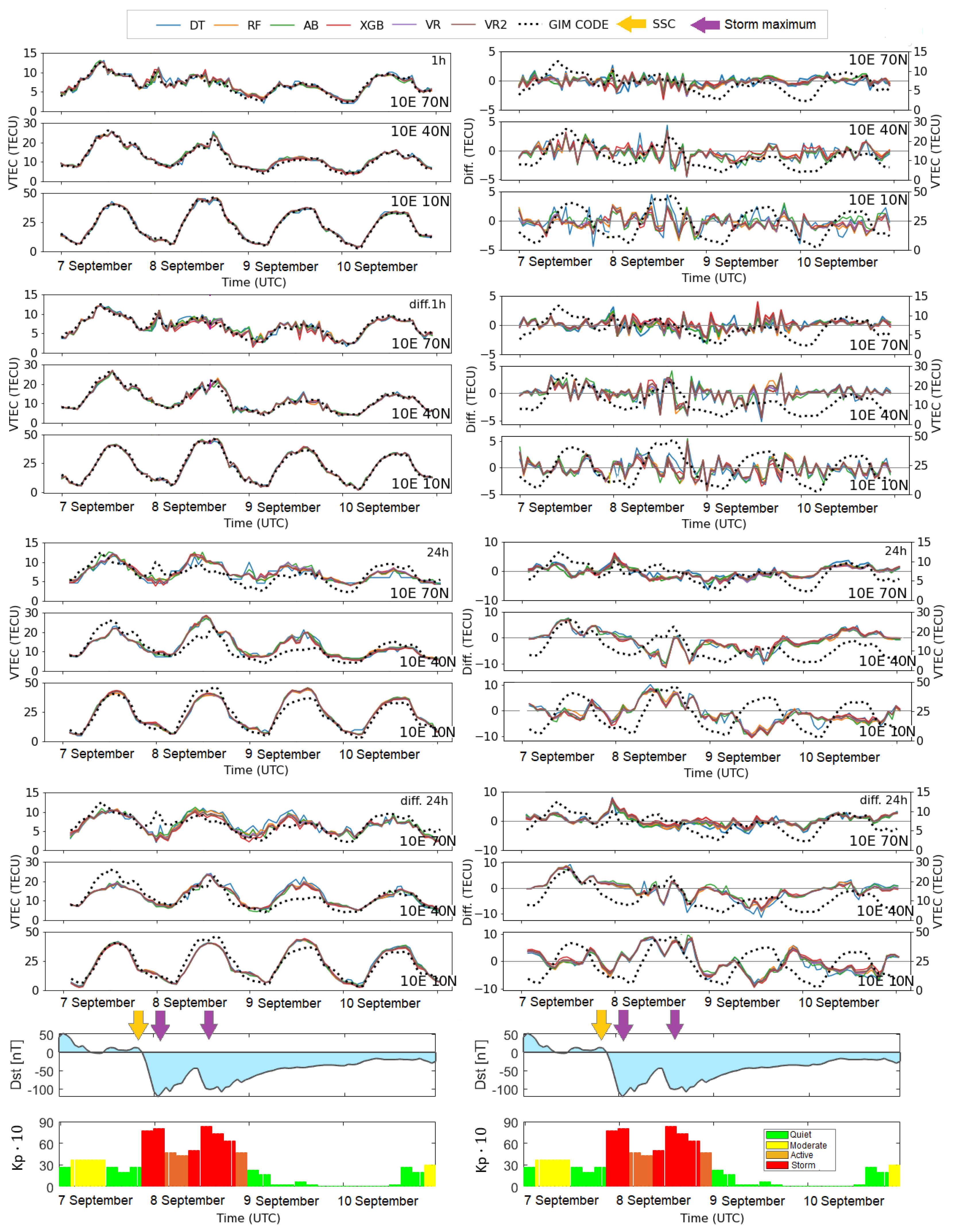
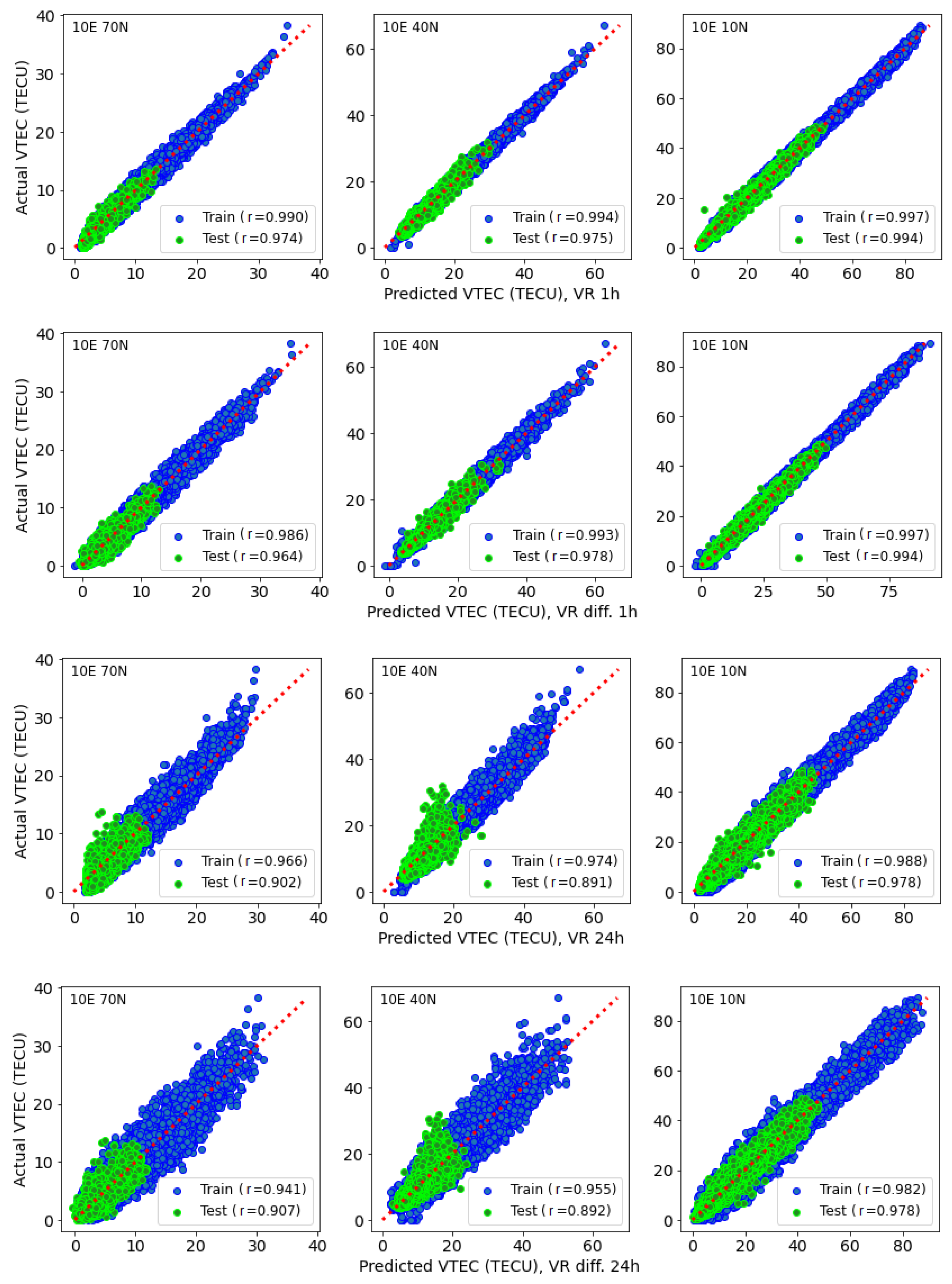
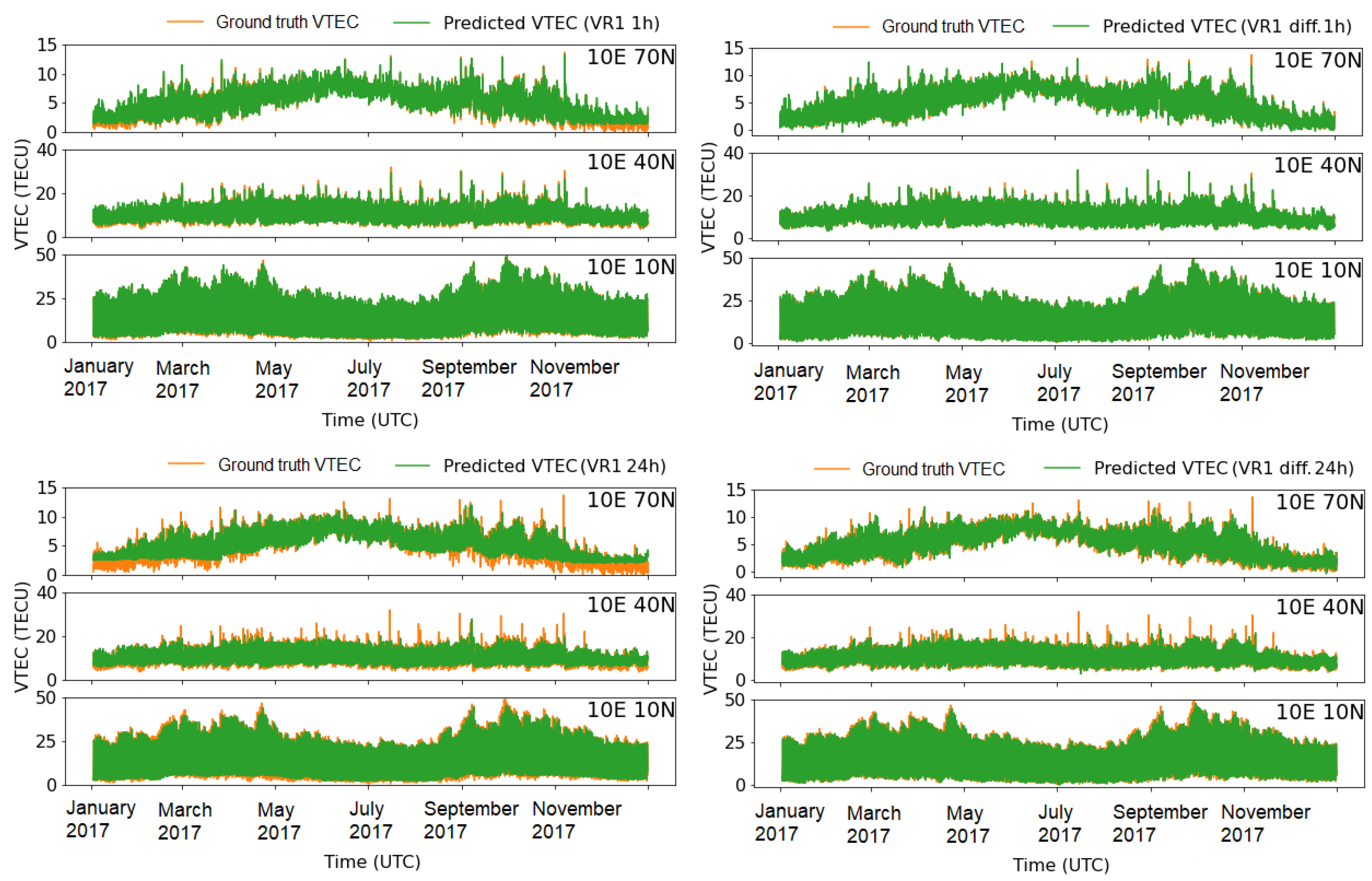
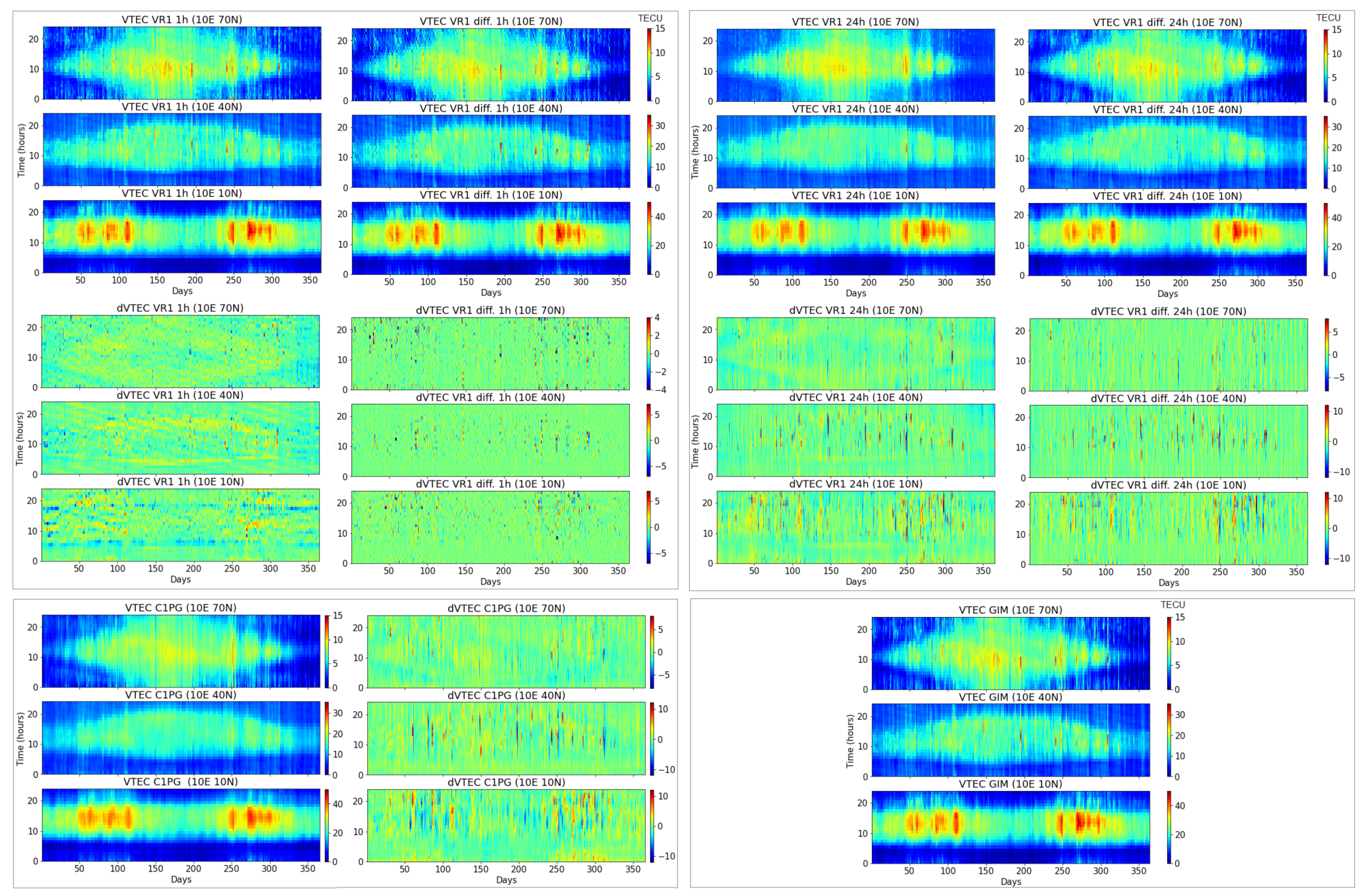
• The new, proposed learning VTEC models can capture variations in electron content consistent with ground truth for both 1 h and 1 day forecasts.
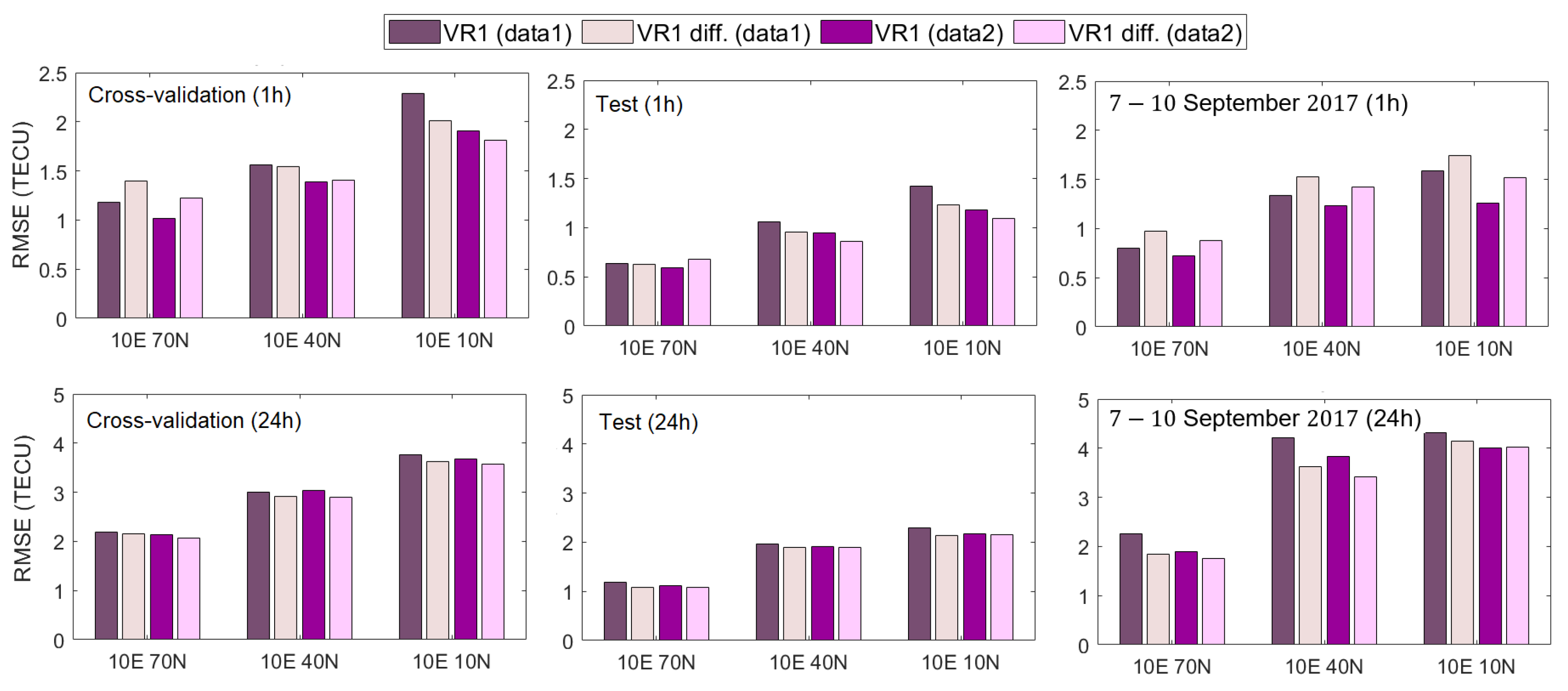
• The ensemble meta-models (VR1 and VR2) improve the VTEC forecasting over each individual model in the ensemble and deliver optimal results.
• Including additional input features, such as moving averages and time derivatives, is beneficial to increase the accuracy of the models.
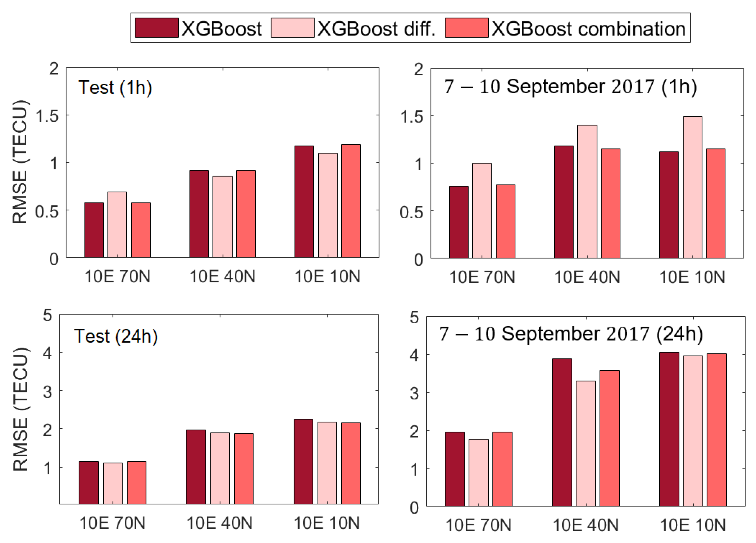
• Data modification in the form of differencing enhances the VTEC model performance for a longer (24-h) forecast, including a geomagnetic storm.

The proposed VTEC models have perspectives to be used as a useful source of information for single-frequency GNSS users to mitigate the ionospheric delay and thereby, directly reduce the ionospheric range error. For instance, the final GIM CODE improves 3D single-frequency position estimates by about 5.5 m, 1 m, and 2.5 m on average in high-, mid-, and low-latitude regions, respectively, compared to the real-time available Klobuchar model [52]. However, considering that the final GIMs are usually provided with a time delay of 1–2 weeks, and the rapid GIMs with 1–2 days [53], their application in real-time is not possible. There are also ultra-rapid GIMs provided with latency of 2–3 h [54] and real-time (RT) GIMs [53,55]. The accuracy of RT GIMs is typically worse than final, post-processed GIMs due to the shorter span of observations, higher noise in carrier-to-code leveling, and difficulty in carrier ambiguity estimation in real-time processing mode [53]. Considering that 1 TECU corresponds to 0.162 m in L1 signal delay, differences between our developed models and the GIM CODE of 1 and 2.5 TECU for the high-latitude, and 2.5 and 5 TECU for the mid-/low-latitude grid points for the 1 h and 1 day forecast, respectively, result in L1 delay difference of about 0.2 m to 0.8 m. This suggests that our 1 h and 1 day VTEC forecast models are expected to improve the GNSS position estimates much more than the Klobuchar model in the studied locations. Thus, forecasted VTEC information can be used to support positioning applications. For a regional or global application, the models should of course be spatially expanded. For operational purposes, the model needs to use VTEC input from the rapid or RT GIMs or estimate it directly from GNSS observations.

The study shows promising results for the application of tree-based ensemble machine learning for VTEC forecasts. This approach has the potential to forecast VTEC in different ionospheric regions during quiet and storm periods. In further work, we plan to extend the models to additional locations to forecast VTEC at the regional or global level. Furthermore, the results support the idea of data importance, which is the core of machine learning and one of the major drivers of machine learning performance. Therefore, future studies will concentrate on further data exploration and modification in order to find the most optimal dataset from which the model can learn, especially over longer forecasting horizons and during space weather. The integration of additional input data that can further characterize space weather in a form useful for learning is intended. In addition, models with longer forecast horizons and multi-epoch predictions are to be developed. An investigation that includes more space weather events will be undertaken and the results should be validated for the latest time period as a new solar cycle is progressing. Another point of interest is the comparison with the neural network-based approach that has so far mainly been used in the area of ionospheric VTEC forecasting. To achieve an objective comparison, the same datasets should be used, and testing should be carried out for the same time period and locations. In addition, the uncertainty of VTEC predictions needs to be quantified, such as in [33], in order to better define the efficiency of the models, provide trustworthy results, and increase the reliability of the VTEC predictions.

References

1. Coster, A.; Komjathy, A. Space Weather and the Global Positioning System. Space Weather 2008, 6, 1–6. [Google Scholar] [CrossRef]
2. Klobuchar, J.A. Ionospheric Time-Delay Algorithm for Single-Frequency GPS Users. IEEE Trans. Aerosp. Electron. Syst. 1987, AES-23, 325–331. [Google Scholar] [CrossRef]
3. Roma, D.; Pajares, M.; Krankowski, A.; Kotulak, K.; Ghoddousi-Fard, R.; Yuan, Y.; Li, Z.; Zhang, H.; Shi, C.; Wang, C.; et al. Consistency of seven different GNSS global ionospheric mapping techniques during one solar cycle. J. Geod. 2017, 92, 691–706. [Google Scholar] [CrossRef] [Green Version]
4. Yuan, Y.; Wang, N.; Li, Z.; Huo, X. The BeiDou global broadcast ionospheric delay correction model (BDGIM) and its preliminary performance evaluation results. Navigation 2019, 66, 55–69. [Google Scholar] [CrossRef] [Green Version]
5. Cander, L.R. Ionospheric Variability. In Ionospheric Space Weather; Springer: Berlin, Germany, 2019; pp. 59–93. [Google Scholar]
6. Nishimura, Y.; Verkhoglyadova, O.; Deng, Y.; Zhang, S.R. (Eds.) Cross-Scale Coupling and Energy Transfer in the Magnetosphere-Ionosphere-Thermosphere SYSTEM; Elsevier: Amsterdam, The Netherlands, 2021. [Google Scholar] [CrossRef]
7. Pulinets, S.; Ouzounov, D. Lithosphere–Atmosphere–Ionosphere Coupling (LAIC) model—An unified concept for earthquake precursors validation. J. Asian Earth Sci. 2011, 41, 371–382. [Google Scholar] [CrossRef]
8. Luo, X.; Du, J.; Lou, Y.; Gu, S.; Yue, X.; Liu, J.; Chen, B. A Method to Mitigate the Effects of Strong Geomagnetic Storm on GNSS Precise Point Positioning. Space Weather 2022, 20, e2021SW002908. [Google Scholar] [CrossRef]
9. Luo, X.; Gu, S.; Lou, Y.; Xiong, C.; Chen, B.; Jin, X. Assessing the Performance of GPS Precise Point Positioning Under Different Geomagnetic Storm Conditions during Solar Cycle 24. Sensors 2018, 18, 1784. [Google Scholar] [CrossRef] [Green Version]
10. Natras, R.; Horozovic, D.; Mulic, M. Strong solar flare detection and its impact on ionospheric layers and on coordinates accuracy in the Western Balkans in October 2014. SN Appl. Sci. 2019, 1, 1–14. [Google Scholar] [CrossRef] [Green Version]
11. Yuan, Y.; Ou, J. An improvement to ionospheric delay correction for single-frequency GPS users—The APR-I scheme. J. Geod. 2001, 75, 331–336. [Google Scholar] [CrossRef]
12. Jordan, M.I.; Mitchell, T.M. Machine learning: Trends, perspectives, and prospects. Science 2015, 349, 255–260. [Google Scholar] [CrossRef]
13. Natras, R.; Schmidt, M. Machine Learning Model Development for Space Weather Forecasting in the Ionosphere. In Proceedings of the CEUR Workshop, Gold Coast, Australia, 1–5 November 2021; Volume 3052. [Google Scholar]
14. Camporeale, E.; Wing, S.; Johnson, J. Machine Learning Techniques for Space Weather; Elsevier: Amsterdam, The Netherlands, 2018. [Google Scholar]
15. Adolfs, M.; Hoque, M.M. A Neural Network-Based TEC Model Capable of Reproducing Nighttime Winter Anomaly. Remote Sens. 2021, 13, 4559. [Google Scholar] [CrossRef]
16. Natras, R.; Goss, A.; Halilovic, D.; Magnet, N.; Mulic, M.; Schmidt, M.; Weber, R. Regional ionosphere delay models based on CORS data and machine learning. Navig. J. Inst. Navig. 2022; in review. [Google Scholar]
17. Tebabal, A.; Radicella, S.; Damtie, B.; Migoya-Orue’, Y.; Nigussie, M.; Nava, B. Feed forward neural network based ionospheric model for the East African region. J. Atmos. Sol.-Terr. Phys. 2019, 191, 105052. [Google Scholar] [CrossRef]
18. Liu, L.; Zou, S.; Yao, Y.; Wang, Z. Forecasting Global Ionospheric TEC Using Deep Learning Approach. Space Weather 2020, 18, e2020SW002501. [Google Scholar] [CrossRef]
19. Srivani, I.; Siva Vara Prasad, G.; Venkata Ratnam, D. A Deep Learning-Based Approach to Forecast Ionospheric Delays for GPS Signals. IEEE Geosci. Remote Sens. Lett. 2019, 16, 1180–1184. [Google Scholar] [CrossRef]
20. Tang, R.; Zeng, F.; Chen, Z.; Wang, J.S.; Huang, C.M.; Wu, Z. The Comparison of Predicting Storm-Time Ionospheric TEC by Three Methods: ARIMA, LSTM, and Seq2Seq. Atmosphere 2020, 11, 316. [Google Scholar] [CrossRef] [Green Version]
21. Kaselimi, M.; Voulodimos, A.; Doulamis, N.; Doulamis, A.; Delikaraoglou, D. Deep Recurrent Neural Networks for Ionospheric Variations Estimation Using GNSS Measurements. IEEE Trans. Geosci. Remote Sens. 2022, 60, 1–15. [Google Scholar] [CrossRef]
22. Ruwali, A.; Kumar, A.J.S.; Prakash, K.B.; Sivavaraprasad, G.; Ratnam, D.V. Implementation of Hybrid Deep Learning Model (LSTM-CNN) for Ionospheric TEC Forecasting Using GPS Data. IEEE Geosci. Remote Sens. Lett. 2021, 18, 1004–1008. [Google Scholar] [CrossRef]
23. Xiong, P.; Zhai, D.; Long, C.; Zhou, H.; Zhang, X.; Shen, X. Long Short-Term Memory Neural Network for Ionospheric Total Electron Content Forecasting Over China. Space Weather 2021, 19, e2020SW002706. [Google Scholar] [CrossRef]
24. Cesaroni, C.; Spogli, L.; Aragon-Angel, A.; Fiocca, M.; Dear, V.; De Franceschi, G.; Romano, V. Neural network based model for global Total Electron Content forecasting. J. Space Weather Space Clim. 2020, 10, 11. [Google Scholar] [CrossRef]
25. Sivavaraprasad, G.; Lakshmi Mallika, I.; Sivakrishna, K.; Venkata Ratnam, D. A novel hybrid Machine learning model to forecast ionospheric TEC over Low-latitude GNSS stations. Adv. Space Res. 2022, 69, 1366–1379. [Google Scholar] [CrossRef]
26. Lee, S.; Ji, E.Y.; Moon, Y.J.; Park, E. One day Forecasting of Global TEC Using a Novel Deep Learning Model. Space Weather 2020, 19, 2020SW002600. [Google Scholar] [CrossRef]
27. Han, Y.; Wang, L.; Fu, W.; Zhou, H.; Li, T.; Chen, R. Machine Learning-Based Short-Term GPS TEC Forecasting During High Solar Activity and Magnetic Storm Periods. IEEE J. Sel. Top. Appl. Earth Obs. Remote Sens. 2022, 15, 115–126. [Google Scholar] [CrossRef]
28. Ghaffari Razin, M.R.; Voosoghi, B. Ionosphere time series modeling using adaptive neuro-fuzzy inference system and principal component analysis. GPS Solut. 2020, 24, 1–13. [Google Scholar] [CrossRef]
29. Zhukov, A.V.; Yasyukevich, Y.V.; Bykov, A.E. Correction to: GIMLi: Global Ionospheric total electron content model based on machine learning. GPS Solut. 2021, 25, 21. [Google Scholar] [CrossRef]
30. Xia, G.; Liu, Y.; Wei, T.; Wang, Z.; Huang, W.; Du, Z.; Zhang, Z.; Wang, X.; Zhou, C. Ionospheric TEC forecast model based on support vector machine with GPU acceleration in the China region. Adv. Space Res. 2021, 68, 1377–1389. [Google Scholar] [CrossRef]
31. Monte-Moreno, E.; Yang, H.; Hernández-Pajares, M. Forecast of the Global TEC by Nearest Neighbour Technique. Remote Sens. 2022, 14, 1361. [Google Scholar] [CrossRef]
32. Wen, Z.; Li, S.; Li, L.; Wu, B.; Fu, J. Ionospheric TEC prediction using Long Short-Term Memory deep learning network. Astrophys. Space Sci. 2021, 366, 1–11. [Google Scholar] [CrossRef]
33. Natras, R.; Soja, B.; Schmidt, M. Machine Learning Ensemble Approach for Ionosphere and Space Weather Forecasting with Uncertainty Quantification. In Proceedings of the 2022 3rd URSI Atlantic and Asia Pacific Radio Science Meeting (AT-AP-RASC), Gran Canaria, Spain, 30 May–4 June 2022; pp. 1–4. [Google Scholar] [CrossRef]
34. Uwamahoro, J.C.; Habarulema, J.B. Modelling total electron content during geomagnetic storm conditions using empirical orthogonal functions and neural networks. J. Geophys. Res. Space Phys. 2015, 120, 11000–11012. [Google Scholar] [CrossRef]
35. Hastie, T.; Tibshirani, R.; Friedman, J. The Elements of Statistical Learning: Data Mining, Inference and Prediction, 2nd ed.; Springer: Berlin, Germany, 2009. [Google Scholar] [CrossRef]
36. Blum, A.; Kalai, A.; Langford, J. Beating the Hold-out: Bounds for K-Fold and Progressive Cross-Validation. In Proceedings of the Twelfth Annual Conference on Computational Learning Theory, Santa Cruz, CA, USA, 7–9 July 1999; Association for Computing Machinery: New York, NY, USA, 1999; pp. 203–208. [Google Scholar] [CrossRef]
37. Arlot, S.; Celisse, A. A survey of cross-validation procedures for model selection. Stat. Surv. 2010, 4, 40–79. [Google Scholar] [CrossRef]
38. Hyndman, R.J.; Athanasopoulos, G. Forecasting: Principles and Practice, 3rd ed.; OTexts: Melbourne, Australia, 2021. [Google Scholar]
39. King, J.H.; Papitashvili, N.E. Solar wind spatial scales in and comparisons of hourly Wind and ACE plasma and magnetic field data. J. Geophys. Res. Space Phys. 2005, 110, 1–9. [Google Scholar] [CrossRef]
40. Breiman, L. Random Forests. Mach. Learn. 2001, 45, 5–32. [Google Scholar] [CrossRef] [Green Version]
41. Freund, Y.; Schapire, R.E. A Decision-Theoretic Generalization of On-Line Learning and an Application to Boosting. J. Comput. Syst. Sci. 1997, 55, 119–139. [Google Scholar] [CrossRef] [Green Version]
42. Chen, T.; Guestrin, C. XGBoost: A Scalable Tree Boosting System. In Proceedings of the 22nd ACM SIGKDD International Conference on Knowledge Discovery and Data Mining, San Francisco, CA, USA, 13–17 August 2016; pp. 785–794. [Google Scholar]
43. Breiman, L.; Friedman, J.; Stone, C.; Olshen, R. Classification and Regression Trees; Taylor & Francis: Abingdon, UK, 1984. [Google Scholar]
44. Wong, T.T.; Yeh, P.Y. Reliable Accuracy Estimates from k-Fold Cross Validation. IEEE Trans. Knowl. Data Eng. 2020, 32, 1586–1594. [Google Scholar] [CrossRef]
45. Friedman, J.H. Greedy Function Approximation: A Gradient Boosting Machine. Ann. Stat. 2001, 29, 1189–1232. [Google Scholar] [CrossRef]
46. Pedregosa, F.; Varoquaux, G.; Gramfort, A.; Michel, V.; Thirion, B.; Grisel, O.; Blondel, M.; Prettenhofer, P.; Weiss, R.; Dubourg, V.; et al. Scikit-learn: Machine Learning in Python. J. Mach. Learn. Res. 2011, 12, 2825–2830. [Google Scholar]
47. Esposito, D. Introducing Machine Learning, 1st ed.; Microsoft Press: Redmond, WA, USA; Safari: Boston, MA, USA, 2020. [Google Scholar]
48. Badeke, R.; Borries, C.; Hoque, M.M.; Minkwitz, D. Empirical forecast of quiet time ionospheric Total Electron Content maps over Europe. Adv. Space Res. 2018, 61, 2881–2890. [Google Scholar] [CrossRef]
49. García-Rigo, A.; Monte, E.; Hernández-Pajares, M.; Juan, J.M.; Sanz, J.; Aragón-Angel, A.; Salazar, D. Global prediction of the vertical total electron content of the ionosphere based on GPS data. Radio Sci. 2011, 46, 1–3. [Google Scholar] [CrossRef] [Green Version]
50. Verkhoglyadova, O.; Meng, X.; Mannucci, A.J.; Shim, J.S.; McGranaghan, R. Evaluation of Total Electron Content Prediction Using Three Ionosphere-Thermosphere Models. Space Weather 2020, 18, e2020SW002452. [Google Scholar] [CrossRef]
51. Imtiaz, N.; Younas, W.; Khan, M. Response of the low- to mid-latitude ionosphere to the geomagnetic storm of September 2017. Ann. Geophys. 2020, 38, 359–372. [Google Scholar] [CrossRef] [Green Version]
52. Wang, G.; Yin, Z.; Hu, Z.; Chen, G.; Li, W.; Bo, Y. Analysis of the BDGIM Performance in BDS Single Point Positioning. Remote Sens. 2021, 13, 3888. [Google Scholar] [CrossRef]
53. Liu, Q.; Hernández-Pajares, M.; Lyu, H.; Goss, A. Influence of temporal resolution on the performance of global ionospheric maps. J. Geod. 2021, 95, 34. [Google Scholar] [CrossRef]
54. Goss, A.; Schmidt, M.; Erdogan, E.; Görres, B.; Seitz, F. High-resolution vertical total electron content maps based on multi-scale B-spline representations. Ann. Geophys. 2019, 37, 699–717. [Google Scholar] [CrossRef] [Green Version]
55. Erdogan, E.; Schmidt, M.; Goss, A.; Görres, B.; Seitz, F. Real-Time Monitoring of Ionosphere VTEC Using Multi-GNSS Carrier-Phase Observations and B-Splines. Space Weather 2021, 19, e2021SW002858. [Google Scholar] [CrossRef]
Figure 1. A small decision tree (maximum depth is 3) for VTEC nowcasting (10°10°) based on input data of temporal information, solar and magnetic activity, and output of VTEC. Inputs x ˜ p are denoted by the indices 0, 1 and 3, which correspond to DOY, HOD and F10.7 index, respectively. Since the tree is small, it takes into account only inputs that have the highest impact on VTEC. Growing a larger tree will result in more nodes that can consider other inputs as well.
Remotesensing 14 03547 g001
Figure 2. Diagrams of bagging and boosting methods.
Remotesensing 14 03547 g002
Figure 3. Evaluation of model performance using time series cross-validation with 20 folds to prevent overfitting and evaluate model performance in a robust way. The final metric is calculated as the average RMSE of every cross-validation iteration.
Remotesensing 14 03547 g003
Figure 4. Flowchart of VTEC machine learning model development from data exploration, selection, and preparation to training and cross-validation until the final machine learning model with the target approximation function is not found. The model is optimized in terms of its performance. Poor performance on training and validation data is the result of high bias, while poor performance on validation data is the result of high variance. They can be solved by increasing or decreasing the model complexity, respectively. The final machine learning model can be used to forecast VTEC on new input data.
Remotesensing 14 03547 g004
Figure 5. Training and validation/test errors as a function of model complexity. Optimal model complexity yields a balanced model that has neither large bias (data underfitting) nor large variance (data overfitting).
Remotesensing 14 03547 g005
Figure 6. Correlation matrix between the model input and ground-truth VTEC. Top: non-differenced data, bottom: differenced data. left: training data (2015–2016), right: training data for Kp ≥ 7.
Remotesensing 14 03547 g006
Figure 7. Percentage of Kp data with the values Kp < 3 , 3 Kp <   4 , 4 Kp <   5 , and Kp   5 denoting quiet, moderate, active and storm conditions, respectively, in the geomagnetic field, over solar cycle 24 (2009–2019) (top left) and for years 2015, 2016 and 2017 (bottom). Top right: Number of hours of the Kp data with values Kp   5 vs. the maximum values of the sunspot number R and the solar radio flux F10.7 (both referring to the right y-axis) from 2009 to 2019.
Remotesensing 14 03547 g007
Figure 8. Number of time series k-folds splits as function of RMSE. Left: RMSE for Decision Tree (DT) and Random Forest (RF) on cross-validation and test datasets for k = 6 and 20. Right: RMSE for the RF model on coss-validation data for k = 6, 10, 20, 30, 40, 50.
Remotesensing 14 03547 g008
Figure 9. RMSE on training and validation data from 1st to 20th k-fold (left). The bar graph represents the average RMSE for all 20 k-folds (right). Top: 1-h, bottom: 24 h forecast. Results are provided for the model VR1 for both non-differenced and differenced (diff.) data.
Remotesensing 14 03547 g009
Figure 10. Relative importance of input variables to VTEC forecast estimated from the Random Forest models. Results are presented for 1 h forecast with non-differenced data (first row) and differenced data (second row), and for 24 h forecast with non-differenced data (third row) and differenced data (fourth row) for high-latitude (left), mid-latitude (middle) and low-latitude (right) VTEC.
Remotesensing 14 03547 g010
Figure 11. Relative importance of input variables to VTEC forecast for geomagnetic storm conditions (Kp ≥ 5) estimated from the Random Forest models. Results are presented for 1 h forecast with non-differenced data (first row) and differenced data (second row), and for 24 h forecast with non-differenced data (third row) and differenced data (fourth row) for high-latitude (left), mid-latitude (middle) and low-latitude (right) VTEC.
Remotesensing 14 03547 g011
Figure 12. The RMSE and correlation coefficient (Corr.) for cross-validation (first column), test (second column) and geomagnetic storm (7–10 September 2017) (third column) datasets, for 1 h and 24 h forecast horizons for Decision tree (DT), Random forest (RF), Adaboost (AB), XGBoost (XGB) and two Voting regressor models (VR1 and VR2). Models trained of differenced data are marked with “diff” The evaluation on the test dataset is a measure of the models’ generalization to new examples.
Remotesensing 14 03547 g012
Figure 13. Relative RMSE change with respect to the persistence (naive) forecast. Top: 1 h forecast, bottom: 24 h forecast. Left: test data (2017), right geomagnetic storm (7–10 September 2017). Models trained of differenced data are marked with “diff.”.
Remotesensing 14 03547 g013
Figure 14. The RMSE for cross-validation (left), test (mid) and geomagnetic storm (right) datasets for 1 h (top) and 24 h (bottom) forecasts for the VR1 model. Models trained with differenced data are marked with “diff”. Data2 refers to data in Table 1, while Data1 comprises Data2 excluding inputs of EMA, VTEC′ and VTEC″.
Remotesensing 14 03547 g014
Figure 15. The RMSE for test dataset (right) and geomagnetic storm (7–10 September 2017) (left) for 1 h (top) and 24 h (bottom) forecasts for the XGBoost model. Models trained using differenced data are marked with “diff”, while “combination” denotes differenced and non-differenced data together, where exponantial moving averages and time derivatives are calculated from non-differenced VTEC, while the model output is non-differenced VTEC.
Remotesensing 14 03547 g015
Figure 16. Left: VTEC values from machine learning models and ground truth VTEC from GIM CODE for the severe geomagnetic storm (7–11 September 2017). Right: Differences between VTEC from machine learning models and GIM CODE VTEC. From top to bottom: 1 h forecast with non-differenced data, 1 h forecast with differenced data, 24 h forecast with non-differenced data, 24 h forecast with differenced data, Dst index, and Kp index ·10. The yellow arrow denotes the sudden storm commencement (SSC) time, while the purple arrows point to two Dst minima, which correspond to the maximum phase of the geomagnetic storms.
Remotesensing 14 03547 g016
Figure 17. Predicted VTEC by the VR1 models vs. ground truth VTEC for training and cross-validation (blue) and test (green) datasets. First row: 1 h forecast with non-differenced data, second row: 1 h forecast with differenced data, third row: 24 h forecast with non-differenced data, fourth row: 24 h forecast with differenced data for high-latitude (left), mid-latitude (middle) and low-latitude (right) VTEC grid points.
Remotesensing 14 03547 g017
Figure 18. Forecasted VTEC by the VR1 model (green) and ground truth VTEC (orange) during year 2017. Top: 1 h, bottom: 24 h forecast. Left: non-differenced data, right: differenced data.
Remotesensing 14 03547 g018
Figure 19. Upper panel left: VR1 model 1 h forecast (top) with non-differenced data (left) and differenced data (right), corresponding VTEC differences ( d V T E C = V T E C G I M V T E C V R 1 ) (bottom). Upper panel right: VR1 model 24 h forecast (top) with non-differenced data (left) and differenced data (right), d V T E C (bottom). Bottom panel left: 1 day predicted GIM CODE (C1PG) (left), d V T E C = V T E C G I M V T E C C 1 P G (right). Bottom panel right: GIM CODE.
Remotesensing 14 03547 g019