Abstract
Satellite hyperspectral remote sensing has gradually become an important means of Earth observation, but the existence of various types of noise seriously limits the application value of satellite hyperspectral images. With the continuous development of deep learning technology, breakthroughs have been made in improving hyperspectral image denoising algorithms based on supervised learning; however, these methods usually require a large number of clean/noisy training pairs, a target that is difficult to meet for real satellite hyperspectral imagery. In this paper, we propose a self-supervised learning-based algorithm, 3S-HSID, for denoising real satellite hyperspectral images without requiring external data support. The 3S-HSID framework can perform robust denoising of a single satellite hyperspectral image in all bands simultaneously. It first conducts a Bernoulli sampling of the input data, then uses the Bernoulli sampling results to construct the training pairs. Furthermore, the global spectral consistency and minimum local variance are used in the loss function to train the network. We use the training model to predict different Bernoulli sampling results, and the average of multiple predicted values is used as the denoising result. To prevent overfitting, we adopt a dropout strategy during training and testing. The results of denoising experiments on the simulated hyperspectral data show that the denoising performance of 3S-HSID is better than most state-of-the-art algorithms, especially in terms of maintaining the spectral characteristics of hyperspectral images. The denoising results for different types of real satellite hyperspectral data also demonstrate the reliability of the proposed method. The 3S-HSID framework provides a new technical means for real satellite hyperspectral image preprocessing.
1. Introduction
With the continuous development of satellite hyperspectral imagers, satellite hyperspectral remote sensing has gradually become an important means for Earth observation [1]. Satellite hyperspectral imagery not only has abundant spatial and spectral information but also an observation efficiency with which airborne or UAV hyperspectral imagery cannot compete. Therefore, satellite hyperspectral imagery has been widely used in smart agriculture [2], urban applications [3], water quality monitoring [4], ecological sustainability [5], and applications in other fields. Compared with natural images, hyperspectral images can simultaneously obtain ground scene information in multiple bands with a low signal-to-noise ratio (SNR), which leads to the inevitable influence of various noises in the process of hyperspectral image acquisition [6]; furthermore, satellite hyperspectral images are also affected by complex space and atmospheric environments [7]. Noise reduces the quality of satellite hyperspectral images and greatly limits their subsequent processing and application [8]. Therefore, denoising prior to satellite hyperspectral image analysis and interpretation is a task of primary importance.
In the past few decades, researchers have proposed a large number of RGB image denoising methods. A common denoising strategy involves directly applying an RGB denoising method to the hyperspectral image denoising task in a band-by-band manner, such as in block-matching and 3D filtering (BM3D) [9], non-local means (NLM) [10], and weighted nuclear norm minimization (WNNM) [11]. Although these methods are relatively simple, correlation between the bands of hyperspectral images is not fully considered, and the original spectral characteristics are often lost in the denoising results [12]. Therefore, denoising methods starting directly from the actual hyperspectral data are becoming increasingly popular for achieving denoising while preserving the spatial and spectral characteristics of hyperspectral data to the maximum possible extent. From this perspective, we can divide the current mainstream methods in the field of hyperspectral image denoising into model- and learning-based methods.
Model-based methods model the noise distribution in the hyperspectral image, and the modeled distribution is then regarded as a prior for accordingly realizing image denoising. Considering the above denoising strategy, it can be seen that the model-based method is highly dependent on the image prior information, including low-rank (LR) [13,14,15,16], total variation (TV) [17,18], and sparse [19,20] priors. Significant research has been conducted, for example, considering the low-rank characteristics of hyperspectral images, and the robust PCA method (RPCA) [21] has been proposed to recover low-rank matrix information. On this basis, low-rank matrix recovery (LRMR) models [13] and hyperspectral restoration (HyRes) [14] have been subsequently proposed. Based on the LR regularization, Xue et al. [15,16] made full use of nonlocal similarity/self-similarity and nonlocal global correlation across spectrum intrinsic priors in order to deal with the lack of spatial constraints for hyperspectral denoising. Similarly, TV regularization is also a common and effective constraint in HSI denoising, and the scientific classical total variation model has been expanded to HSI [17]. Structure tensor TV (STV) [22] has been proposed, which utilizes the low rank of gradient vectors in local regions. Then, spatial–spectral TV (SSTV) [18] has been proposed to preserve spatial–spectral information by applying TV regularization to the HSI gradient in the spectral direction. Furthermore, Fei et al. [23] integrated low-rank prior and spatial–spectral total variation with directional information (SSDTV) for HSI restoration.
In general, the spatial and spectral characteristics of hyperspectral images are essentially used by methods based on the model prior, in which the denoising performance is obvious. Most model-based approaches, however, still have unavoidable problems. On one hand, in the process of modeling the distribution of hyperspectral images or noise, there are complex mathematical derivation and optimization problems, resulting in a sharp increase in the calculation volume. This not only makes the denoising of hyperspectral images very inefficient but also often fails to adequately maintain the texture structure when the noise is relatively severe. On the other hand, prior models are often non-convex optimization problems that require a large number of numerical iterations and parameter adjustments when manually given parameters, which also limits further improvement of the denoising performance. More importantly, model-based methods are often trained and modeled concerning a specific type of noise, such that their application in actual hyperspectral image denoising tasks is limited.
In contrast to model-based methods, learning-based methods are not dependent on manual priors and learn the hyperspectral image features through data-driven, to realize hyperspectral image denoising. In other words, compared to the above traditional methods, different network designs can better adapt to the noise in real data to achieve a better denoising effect. Following their rapid development, the use of learning-based methods has become a mainstream hyperspectral image denoising strategy. Learning-based methods can be further divided into supervised learning denoising methods and unsupervised/self-supervised learning denoising methods, according to whether external training samples are needed.
The focus of supervised learning denoising methods is to learn the non-linear potential mapping between noisy and clean hyperspectral images in order to realize hyperspectral image denoising. Xie et al. [24] first introduced the trainable non-linear reaction diffusion (TNRD) model for hyperspectral image denoising based on the deep learning denoising strategy for gray images, and the proposed model was shown to effectively remove Gaussian noise. However, this method does not make full use of the correlation between the bands of hyperspectral images, and spectral details may be lost. To retain the spectral characteristics, Xie et al. [25] used a denoising convolutional neural network (CNN) model for hyperspectral image denoising. Through residual learning, the spectral information contour was effectively retained. Then, the strategy of using key bands for spatial initialization and assisting in denoising was designed [26], which further solved the problem of spectral distortion after denoising. However, deep learning denoising frameworks based on natural images cannot make good use of the inherent spatial–spectral advantage of hyperspectral data. Therefore, various deep learning denoising frameworks based on spatial–spectral characteristics have been proposed. Yuan et al. [27] proposed a denoising framework based on spatial–spectral learning, named HSID-CNN, which fuses the spatial characteristics of a single-band extracted using a 2D-CNN with the spectral characteristics of adjacent bands obtained by a 3D-CNN. To avoid the need for HSID-CNN to train different models for different noise intensities, Maffei et al. [28] proposed a new model, called HSI single denoising CNN (HSI-SDeCNN), which can consider both spatial and spectral correlations. To better preserve the spatial and spectral details of hyperspectral data, researchers have combined image and depth priors to give full play to their respective advantages, consequently achieving satisfactory denoising results. For example, by using the low-rank and local self-similarity priors of hyperspectral data in the spectral domain and combining them with the spatial depth prior extracted using a CNN, the mixed noise has been removed, thus providing an improved denoising performance [29,30,31,32]. Given the great success of attention mechanisms in the fields of image recognition, target detection, and other computer vision applications, researchers have proposed the use of a deep learning denoising framework based on an attention mechanism to further utilize the global dependence and correlation between spatial and spectral information in hyperspectral data. In this approach, the attention module is added to the spatial domain and spectral channel, such that the neural network is more focused on learning the noise characteristics, and the denoising effect with respect to mixed noise is obvious [33,34,35,36].
It can be seen from the above that supervised deep learning denoising methods perform better, both in terms of learning the noise characteristics and utilizing and maintaining the spatial–spectral characteristics. As such, they can be said to have achieved satisfactory denoising results. However, most supervised learning denoising methods require a significant amount of supervised training; that is, the denoising network must be trained using clean/noisy hyperspectral image pairs to achieve an optimal denoising performance. However, the acquisition of clean/noisy hyperspectral image pairs is very difficult, which greatly limits the generalization ability of supervised learning denoising methods and their robustness in denoising real data.
To solve this problem, some scholars have studied unsupervised/self-supervised learning methods based directly on the actual data. However, compared with the denoising methods based on supervised learning, only using single images for denoising poses many challenges, such as the automatic construction of training image pairs, high-quality feature learning, effective loss function construction, and so on. Scholars have made a series of attempts to address these issues. Deep image prior (DIP) [37] has been widely used in natural image denoising. Sidorov et al. [38] proposed deep hyperspectral prior (DHP) based on DIP without any external training samples, which can use a CNN to learn the image prior of hyperspectral image data for hyperspectral image denoising, restoration, and super-resolution tasks. To overcome the semi-convergence of the DIP method, Luo et al. [39] proposed the spatial–spectral constrained deep image prior (S2DIP) framework. Imamura et al. [40] proposed a self-supervised learning hyperspectral image restoration method based on the separable image prior (SIP), in which separable convolution is used to extract image prior from hyperspectral data, and constructed the training sample dataset needed for self-supervised learning. Fu et al. [41] combined a model-based method with a deep learning method, constructed clean/noisy training pairs using single hyperspectral image data, and trained a denoising network with an HSI denoising model based on sparse representation. To deal with real hyperspectral image denoising, Wang et al. [42] proposed a self-supervised hyperspectral image denoising network, named SHDN, which can extract a single HSI data noise sample through a noise estimator and form a clean/noisy training pair by combining the noise sample with the filtered clean band, which can then be used for CNN denoising network training. Qian et al. [43] proposed a two-stage self-supervised denoising network based on the similarity of adjacent bands of hyperspectral data.
The above works have provided many ideas for the study of unsupervised/self-supervised learning denoising. It can be seen, from these algorithms, that the spatial and spectral information of the hyperspectral image is still indispensable for unsupervised/self-supervised hyperspectral image denoising; however, we focus not only on the retention effect of spatial domain features but also on maintaining the spectral domain features after denoising. Inspired by the natural image denoising framework Self2Self [44], we make full use of the spectral characteristics of hyperspectral images and propose a self-supervised denoising method for real satellite hyperspectral imagery. Furthermore, a spectral consistency constraint is added to the model loss of 3S-HSID to maintain the spectral characteristics. The 3S-HSID framework can deal with the complex noise in real satellite hyperspectral images, including Gaussian noise, salt and pepper noise, and bad lines. We summarize the main contributions of the proposed algorithm as follows:
- The 3S-HSID framework is a strict self-supervised denoising method. A Bernoulli sampling of a single hyperspectral image can be used to construct the clean/noisy image pairs required for training. No external training data are needed, and the noise situation of the hyperspectral data is not estimated. No clean band is needed as a reference, and no spatial adjacent bands are needed for auxiliary denoising. All hyperspectral bands can be denoised at the same time, especially in the case of real satellite hyperspectral images;
- The 3S-HSID framework establishes a global spectral consistency constraint between the model input and output, which maximizes the recovery of spectral characteristics of ground objects while restoring spatial information;
- The 3S-HSID framework can be applied in different platforms, at different spatial resolutions, and in different spectral resolution satellite hyperspectral image denoising experiments, and the different types of noise removal effects are remarkable, thus providing a new solution for the denoising of real satellite hyperspectral images.
The remainder of this article is organized as follows. Section 2 introduces the experimental datasets, which include the simulated noisy HSI datasets and multi-resolution real satellite HSI datasets, and describes the proposed self-supervised satellite HSI denoising network. Section 3 analyzes the experimental results of the proposed method and the compared methods. Our conclusions are summarized in Section 4.
2. Materials and Methods
2.1. Datasets
To verify the robustness of 3S-HSID, we chose a public hyperspectral dataset named Pavia University as the simulated data. The common noises of satellite hyperspectral images, such as Gaussian noise, salt and pepper noise, and bad lines, were loaded into simulated hyperspectral data with different intensities, and 3S-HSID was used to denoise the simulated data. To verify the generalization ability of the 3S-HSID algorithm, satellite hyperspectral images with different sensors, spatial resolutions, and spectral resolutions were adopted in this paper, including GF-14, ZH-1, and PRISMA satellite hyperspectral datasets. All data were normalized to the range 0–1 before denoising. The details of the above datasets are described as follows:
- 1.
- The Pavia University dataset is a commonly used airborne hyperspectral dataset obtained by the ROSIS sensor with 115 bands. To increase the possibility of its application in all kinds of noise simulations, we used only 87 bands, and the data size was 256 × 256.
- 2.
- GF-14 is an optical stereo mapping satellite arranged by the National Science and Technology Major Project of the High-Resolution Earth Observation System, which was launched into orbit on 6 December 2020. The satellite hyperspectral imager carried by GF-14 can obtain hyperspectral images with a spatial resolution of 5 m in visible to near-infrared wavelengths and of 10 m in the short-wave infrared wavelength, with 70 and 30 bands, respectively. The data used in this paper were captured by GF-14 in 2021, and radiation and atmospheric corrections were carried out before denoising.
- 3.
- The Zhuhai-1 remote sensing micro–nanosatellite constellation is a commercial remote sensing micro–nanosatellite constellation constructed and operated by Zhuhai Obit Aerospace Science and Technology Co., Ltd., Zhuhai, Guangdong, China. The Zhuhai-1 constellation contains different types of micro- and nano-satellites, including video satellites, high-resolution optical satellites, hyperspectral satellites, SAR satellites, and infrared satellites. Among them, the hyperspectral satellite (ZH-1) was launched into orbit on 26 April 2018. Its orbit height is 500 km, the imaging width is 150 km, the spatial resolution is 10 m, the spectral resolution is 2.5 nm, the wavelength range is 400–1000 nm, and the number of bands is 32. The data used in this paper are OHS captures of Shenzhen, China, on January 31, 2021. Before denoising, radiation and atmospheric corrections were carried out.
- 4.
- The hyperspectral pioneer and application mission (PRISMA) satellite was launched into orbit by the Italian Space Agency on 21 March 2019. Its orbit height is 620 km, which allows complete coverage of Earth. The imaging width of PRISMA is 30 km. Hyperspectral images with a spatial resolution of 30 m can be obtained in orbit. The spectral resolution is lower than 12 nm, and the number of imaging bands in the visible and near-infrared ranges is 66 and 173, respectively. At present, PRISMA data can be freely downloaded, and the official hyperspectral data at L0–L2 levels are provided.
2.2. Satellite Hyperspectral Image Degradation
Although satellite hyperspectral images are affected by various types of noise during acquisition, the degradation model can be simply expressed as
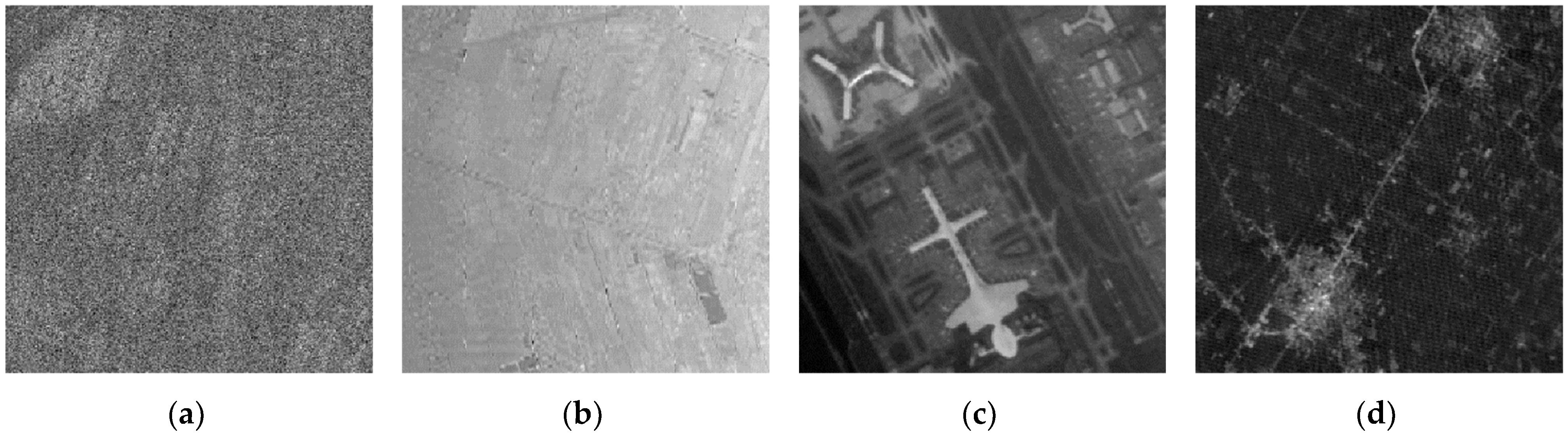
where represents a band containing noise in hyperspectral data, represents the band data that are not interfered with by noise, and represents the set of various types of noise. As shown in Figure 1, the bands of satellite hyperspectral images may be affected by different types of noise, such as Gaussian noise, salt and pepper noise, and bad lines. The noise pollution in different bands often differs in intensity and type, which poses great challenges and uncertainties when carrying out hyperspectral image denoising.

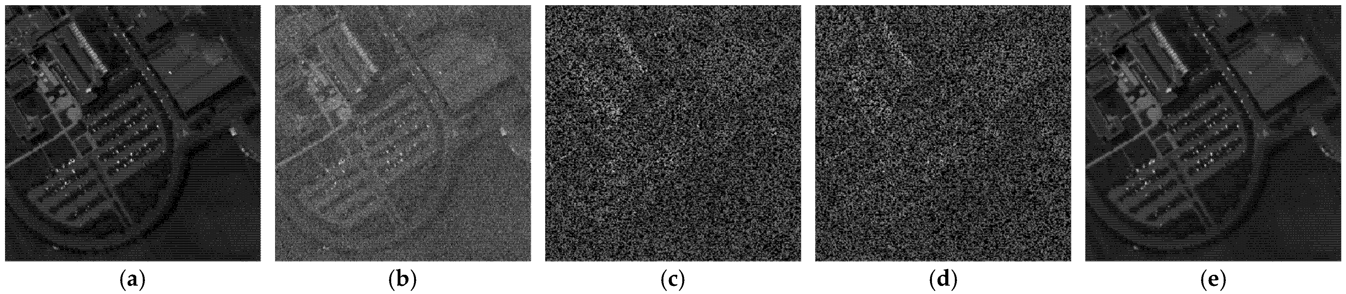
Figure 1.
Noise in real satellite hyperspectral imagery: (a) GF-14 visible to near-infrared HSI (band 5); (b) GF-14 short-wave infrared HSI (band 1); (c) ZH-1 HSI (band 1); and (d) PRISMA HSI (band 66).
2.3. 3S-HSID Network Framework
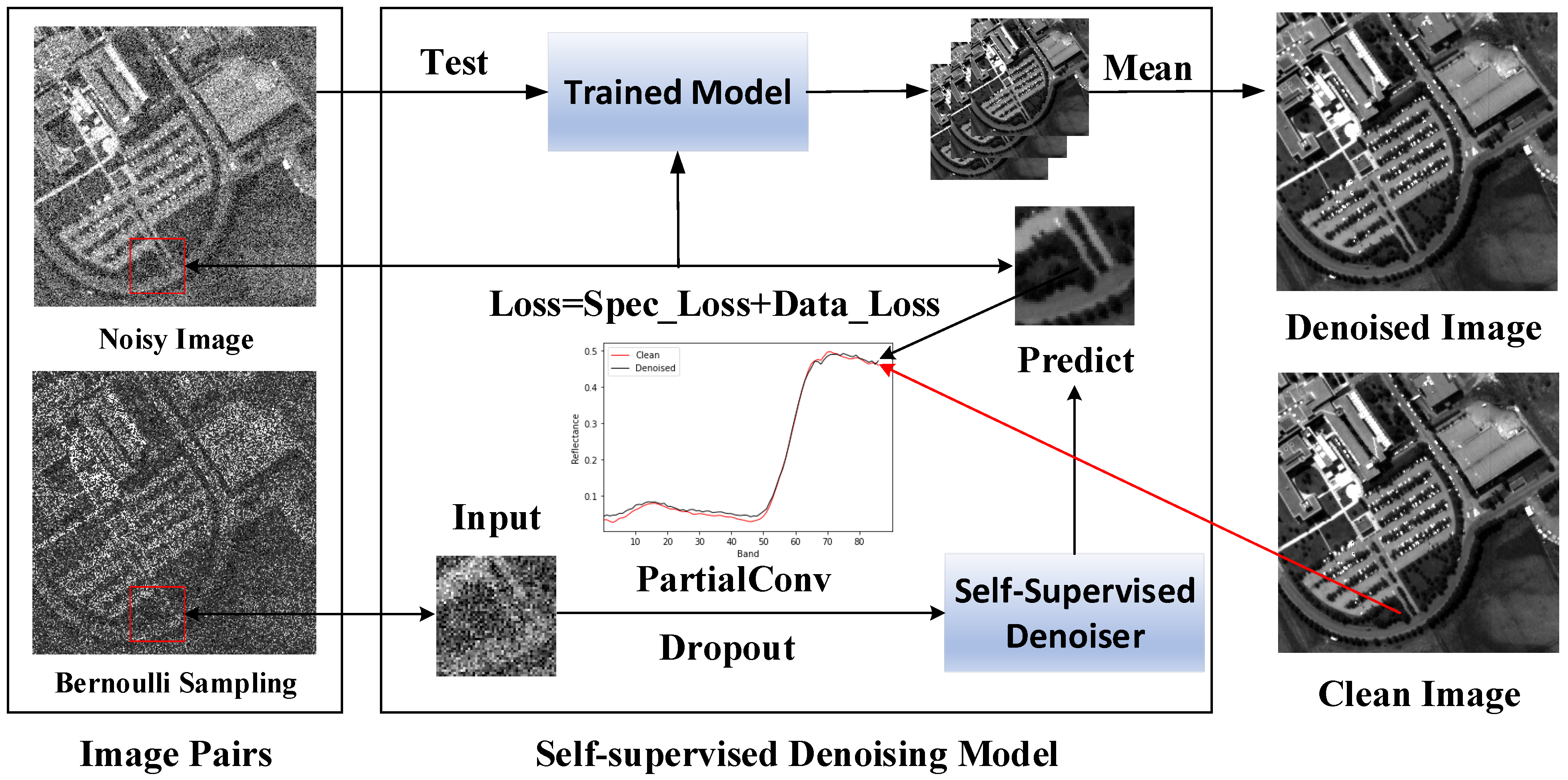
We propose a self-supervised learning-based denoising algorithm for satellite hyperspectral images, referred to as 3S-HSID. The framework is depicted in Figure 2. The 3S-HSID framework is a self-supervised learning strategy that does not require external training data support. The input data are used to directly construct a clean/noisy image pair in order to robustly denoise a single satellite hyperspectral image. The denoising framework details are explained individually in the following.
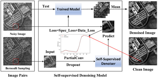
Figure 2.
Network architecture of 3S-HSID including constructed image pairs and self-supervised denoising model.
2.4. Dropout Strategy
In essence, denoising is a typical regression problem representing the inverse process of data contamination by noise. In deep learning, the mean squared error () is generally used to measure the prediction accuracy of a regression model. The can be simply expressed as
where is an element value in the sample, and is the model predicting value of the element . It can be seen that the is closely related to the sample. Furthermore, when we use sample statistics to predict some parameters of the population, we expect to obtain the sampling distribution of the sample statistics. At this time, any estimation of the is based on the function of sample data, such that the can be rewritten, in terms of the sample variance and bias, as
In the case of unbiased estimation, the is equivalent to the variance, which also reflects the difference between the predicted value and the real value in the model. In the process of supervised training, when there are too many model parameters and the training dataset is too small, the problem of model overfitting will occur. At this time, a large number of independent samples can be used to train the model. With an increase in sample size, the variance—and, thus, the —will continue to decrease, such that the predicted value becomes close to the real value. However, when we only use a single hyperspectral image to train the network, the problem of insufficient training data will be very obvious. A core issue in this case is how to minimize the and successfully predict its true value.
In deep learning, when the number of training samples is small, the neural network cannot fully describe the training problem, which will lead to overfitting of the model. Dropout [45] is a commonly used regularization method to address the overfitting problem. Dropout hides some neural network nodes in the training process, according to a certain probability, which is equivalent to introducing uncertainty in model training [46]. The predicted value of the model after dropout may also have some independent statistical characteristics, thus reducing the variance between the model prediction and the real value. Similarly, under the same training sample conditions, dropout can result in the predicted value of the model being closer to the real value. In other words, the will decrease as the training time increases.
2.5. Training Scheme
The 3S-HSID framework is a network architecture based on self-supervised learning. It is very important to construct clean/noisy image pairs for model training. For most deep learning denoising methods, the network is trained using a large number of clean/noisy image pairs, such that the network can learn the mapping relationship between noisy images and clean images to the maximum possible extent to realize denoising. In the case of 3S-HSID, the training data source is only the input single hyperspectral image data, for which there is no corresponding clean image. Inspired by Self2Self, we used Bernoulli sampling to process the input data and construct the clean/noisy image pairs required for self-supervised training. The Bernoulli matrix can be defined as
where a random matrix with the value range of is generated, and the Bernoulli probability is determined. According to the comparison between the element value of the random matrix and , the Bernoulli matrix is generated; and represent the width and height of the input hyperspectral image, respectively, and represents the number of bands. The matrix is generated according to the binary Bernoulli sampling principle and follows the Bernoulli distribution. Then, we can construct clean/noisy image pairs through Bernoulli sampling. However, the image pairs based on Bernoulli sampling are completely different from those in supervised learning. The noisy image in the image pair comes from the Bernoulli sampling example, while the clean image is the data discarded by sampling. We do not directly establish the mapping relationship between the two, but we take the noise data as the input and obtain the prediction results after denoising. The prediction results and the data discarded by sampling are used to establish a functional relationship. Here, the Bernoulli sampling instance and the part discarded by sampling are expressed as and , according to Equations (5) and (6), respectively:
where represents the point multiplication operation between matrices, represents the given input hyperspectral data, and represents the Bernoulli sampling matrix. The 3S-HSID process from input to output is shown in Figure 3.
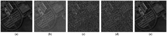
Figure 3.
HSI processing process: (a) clean HSI; (b) simulated noise HSI; (c) Bernoulli sampling results as model input; and (d) Bernoulli sampling discard result; and (e) output result.
A different Bernoulli sampling results from different noise data and for a series of noise hyperspectral image pairs (, ). Such image pairs are needed for self-supervised training; that is, the model takes as the input data, and the model recovers based on and obtains the model output .
With the increase in sampling, the number of training samples will be greatly enriched, and each Bernoulli sampling itself can also be regarded as a dropout operation in the network to further improve the model’s fitting ability. On this basis, we carry out data enhancement operations on the original input data, which mainly consist of multi-angle rotation and vertical/horizontal flip operations. Using different combinations, up to 14 transformation enhancements can be carried out on the original input data .
2.6. Model Structure
We proposed a self-supervised hyperspectral image denoising method, and the structure of this model is shown in Table 1.

Table 1.
Network structures of 3S-HSID.
It can be seen from Table 1 that the 3S-HSID network is an encoder–decoder network architecture based on the U-Net structure. The network encoding stage consists of nine encoder blocks, while the decoding stage consists of five decoder blocks. In the decoding stage, a residual connection is used to prevent the gradient of the deep network from disappearing. The input data are single hyperspectral image data affected by noise with dimensions of w × h × c. Before encoding, the input data are non-linearly mapped to -dimensional data by two partial convolution modules. The subsequent encoder blocks are composed of a partial convolutional layer, an unsaturated activation function (LeakyReLU), and a maximum pooling layer. The maximum pooling layer stride is 2, and the consistency of data size before and after convolution is ensured by adjusting the stride of the partial convolution. After all the encoder modules, the output high-dimensional feature data have dimensions of . Before each decoder module, the up-sampling operation doubles the size of the high-dimensional feature data. The first four decoder modules are composed of two 2D convolutional layers and two unsaturated activation functions (LeakyReLU). On this basis, the last decoder module adds a 2D convolutional layer and a saturated activation function (Sigmoid). The input data for each decoder module are connected by residuals.
To retain the original image information, the last decoder module connects the data from before the Bernoulli sampling with the output of the previous decoder module. Dropout is used in all convolutional layers of the decoder modules in order to prevent training overfitting due to the use of single hyperspectral image data training.
2.7. Loss Function
Combined with the previous analysis of in Section 2.4, when the between the predicted value and the data discarded by sampling is minimized, we believe that the model produces the most accurate prediction for the data discarded by sampling, and the loss function can be described by
where denotes the number of data points discarded by Bernoulli sampling. It can be seen from Equation (7) that 3S-HSID only uses the data discarded by Bernoulli sampling when calculating the loss function and reintroduces uncertainty into the model, which increases the model stability.
In the hyperspectral image denoising task, we focus not only on the retention effect of spatial domain features but also on maintaining the spectral domain features; that is, the spectral consistency between the prediction results and the input data should be maintained. Therefore, a spectral consistency constraint is added to the model loss of 3S-HSID, in which the spectral angle is used to measure the similarity between the predicted and original spectra, such that the spectral characteristics of the pixels corresponding to the model output and the original input data are consistent when restoring the spectral detail characteristics. We use the spectral angle chord as the spectral similarity measure to calculate , and the spectral loss function can be expressed as
The entire model loss function can be expressed as
where the calculation object of is all pixels, and that of is only on . Therefore, can be understood as a local optimum constraint, while is more similar to a global optimum constraint.
2.8. Denoising Scheme
We know that noise in real data is often a superposition of various types of noise. Each type of noise can be assumed to be a random variable subject to a certain probability distribution, such that the real noise can be expressed as
where is the noise we observe, and is random noise that obeys a certain probability distribution; notably, we assume the are independent and of mean zero. According to the central limit theorem, when different types of noise accumulate in large numbers, will tend to a normal distribution (i.e., a Gaussian distribution). When we use a deep neural network to denoise the noise data, the neural network model is usually regarded as a conditional distribution probability model, expressed as
where is the input noise data, is the data predicted by the network model, and denotes the network weights. However, the value predicted by the model, , contains Gaussian noise (with mean zero). A series of predicted values are obtained by multiple predictions, and some Gaussian distributions are then obtained. Therefore, the model actually predicts the mean values of these Gaussian distributions. The average value of the multiple prediction results is the final prediction result of the model:
where is the final prediction result, and denotes the number of predictions.
From the analysis in Section 2.5, it can be seen that the neural network model obtained by training is subject to the Bernoulli distribution. Therefore, in the test stage, the Bernoulli probability is still used to scale the neural network model obtained in the training stage in order to generate multiple denoising results with independent distributions. In the training stage, we use the network training model to predict different Bernoulli sampling examples many times. According to Equation (12), we can obtain the result of 3S-HSID denoising on input data using the obtained weights; that is, we expect a clean image.
The use of dropout, Bernoulli sampling, partial convolution, and other operations allowed us to achieve satisfactory results in the self-supervised denoising of a single natural image. Inspired by this, we comprehensively analyzed the characteristics of hyperspectral data. Based on the above strategies, we incorporated the spectral consistency prior to form a self-supervised denoising network for real satellite hyperspectral imagery. To the best of our knowledge, this is a novel hyperspectral image self-supervised learning denoising framework, especially for real satellite hyperspectral images with different platforms, spatial resolutions, and spectral resolutions. As it does not require additional training data, it has a high practical application value.
3. Results
3.1. Experimental Setup
In the process of 3S-HSID denoising, the relevant hyperparameters must first be set, which are detailed as follows. The input data were full-band hyperspectral data, and satisfactory denoising results could be obtained after one round of processing. When Bernoulli sampling the input data, the sampling probability was set to 0.5. All partial convolution and standard convolution kernel sizes in the 3S-HSID network framework were used with a stride of one and padded with zero to ensure that the size did not change before and after convolution. In the framework, LeakyReLU was selected as the activation function, and its hyperparameter value was 0.1. A BN layer is added before the LeakyReLU layer in the encoding stage in order to ensure the stability of the network. For dropout, the random discard probability was set to 0.5. We chose Adam as the optimizer for model training, for which the learning rate was set to 10−5. It should be noted that in the simulation experiment the iteration number of 3S-HSID in the training and testing process was adaptively determined according to the optimal denoising results, and the iteration number for real data was determined according to the iteration number in the simulation experiment. The 3S-HSID framework processes a single HSI without parallel computation. Suppose the iteration number of 3S-HSID is 10,000, the implementation takes around 50 min to process an HSI of size on average. Our computer hardware environment was an RTX 2080Ti GPU, and the software environment was Python 3.6 + PyTorch 1.8.1.
To simulate the noise in real satellite hyperspectral images as much as possible, we designed Gaussian noise, salt and pepper noise, bad line, and other noise types and simulated the complex noise in the PaviaU hyperspectral data through the fusion of different types of noise. The setting of the simulated noise is as follows:
- Case 1 (including Case 11 and Case 12): Adding Gaussian noise with the same mean intensity to each band of the original data, where the standard deviation of the Gaussian noise is ;
- Case 2: Adding Gaussian noise with a different mean intensity to each band of the original data, where the standard deviation range of the Gaussian noise is
- Case 3: Based on Case 2, salt and pepper noise of different proportions is added to 30% of the bands in the original data, where the proportion range of the salt and pepper noise is ;
- Case 4: Based on Case 2 and Case 3, bad lines of different proportions are added to 30% of the bands in the original data, where the proportion range of the bad lines is .
The mixed noise in real hyperspectral images was simulated through the random occurrence of concentrated noise, as shown in Figure 4.
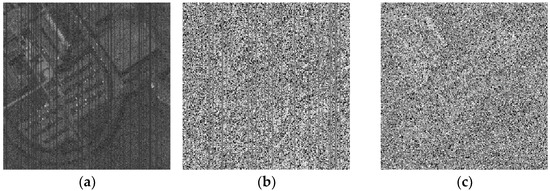
Figure 4.
Noise simulation in different bands of PaviaU hyperspectral data, such as: (a) Gaussian noise in band 19; (b) Gaussian noise, salt and pepper noise, and bad lines in band 30; and (c) Gaussian noise and salt and pepper noise in band 77. Different bands are affected by varying degrees of noise.
3.2. Simulation Denoising Experiment
To verify the performance of 3S-HSID denoising, we selected seven previously published hyperspectral image denoising algorithms that have relevant operating procedures for comparison, including the traditional block-matching and 4D filtering (BM4D) method [47]; model-based methods, including low-rank matrix recovery (LRMR) [13], parameter-free hyperspectral restoration (HyRes) [14], and L1HyMixDe [48]; and unsupervised/self-supervised learning-based single hyperspectral image denoising methods, including deep hyperspectral prior (DHP) [38], separable image prior (SIP) [40], and Stein’s unbiased risk estimate convolutional neural network (SURE-CNN) [49]. All algorithms used for comparison were applied according to the information published by their respective authors.
To evaluate the performance of 3S-HSID denoising and compare it with other state-of-the-art algorithms, we used several commonly used quantitative indicators to evaluate the denoising results. Due to the ideal reference data, the comparison between the different algorithms was considered very fair.
- PSNR, SSIM
Peak signal-to-noise ratio (PSNR) and structural similarity (SSIM) are commonly used indicators for evaluating the quality of image reconstruction in ordinary image processing. For hyperspectral images, we only need to calculate the PSNR and SSIM band-wise for two hyperspectral images, and then take the average values to obtain the overall PSNR and SSIM for hyperspectral images. The higher the PSNR and SSIM values, the better the denoising performance.
- SAM
Spectral angle mapper (SAM) is a unique evaluation index by which to measure the spectral consistency of hyperspectral data. By calculating the spectral distance between the spectral curves of the corresponding pixels of two hyperspectral images and then taking the average value of the calculation results of all pixels, the SAM value of the whole image can be obtained. The lower the SAM value, the better the denoising performance.
Based on the above experimental settings, we used the PaviaU hyperspectral data as the ideal data for testing different types of noise effects, and the various denoising algorithms were applied for their recovery. Table 2 provides the recovery results regarding the effect of various denoising algorithms under different noise types. The best results are marked with double underscores, and sub-optimal results are marked with a single underscore. It can be seen from the quantitative results that, in most cases, the lowest SAM value was achieved by 3S-HSID; that is, the recovery effect due to the spectral consistency constraint on spectral characteristics was obvious. In terms of PSNR and SSIM indicators, the proposed approach presented similar results to the model-based algorithms and had obvious advantages when compared to self-supervised learning algorithms, such as DHP-2D and SIP. SURE-CNN is one of the most advanced unsupervised denoising algorithms; our performance in PSNR and SSIM are close to SURE-CNN. Nonetheless, our algorithm is better than SURE-CNN in visual effects of denoising results.
Table 2.
Denoising results of PaviaU hyperspectral simulation data.
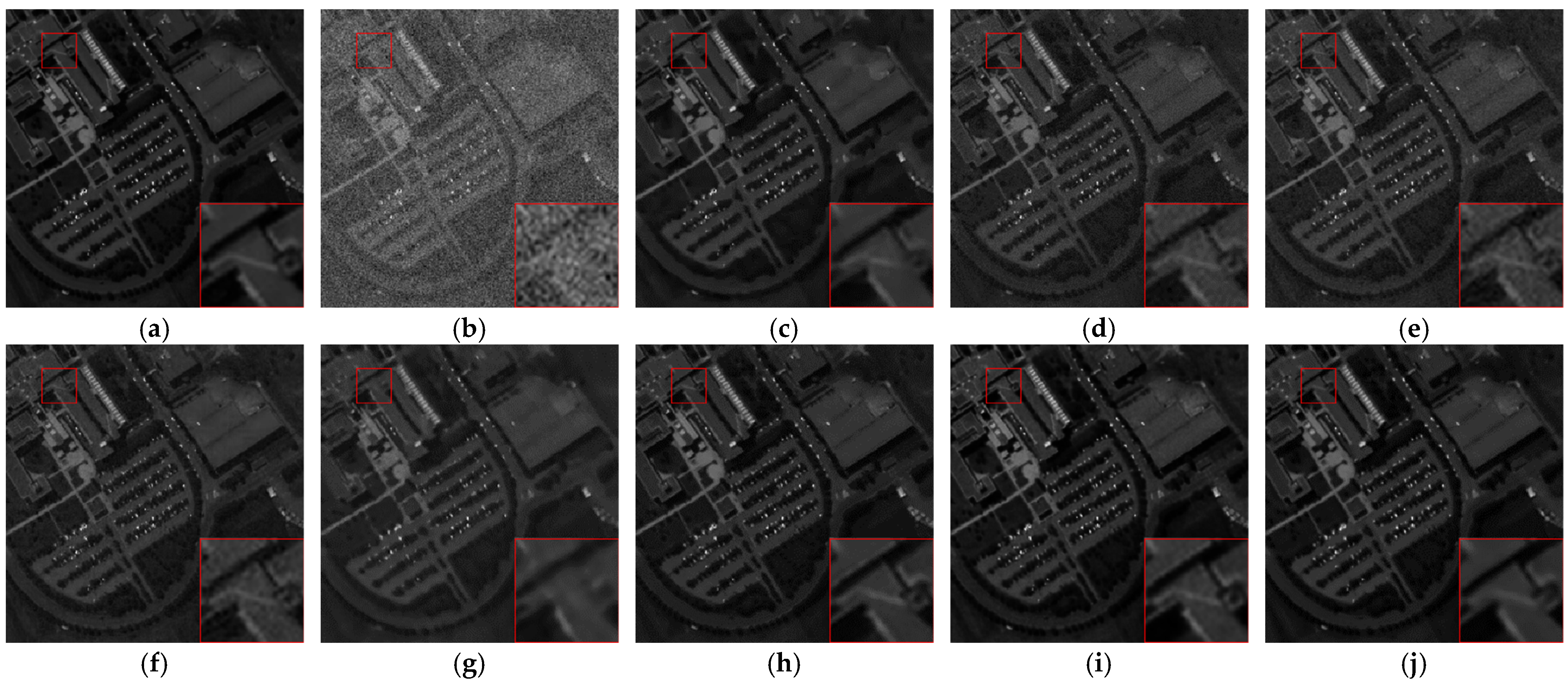
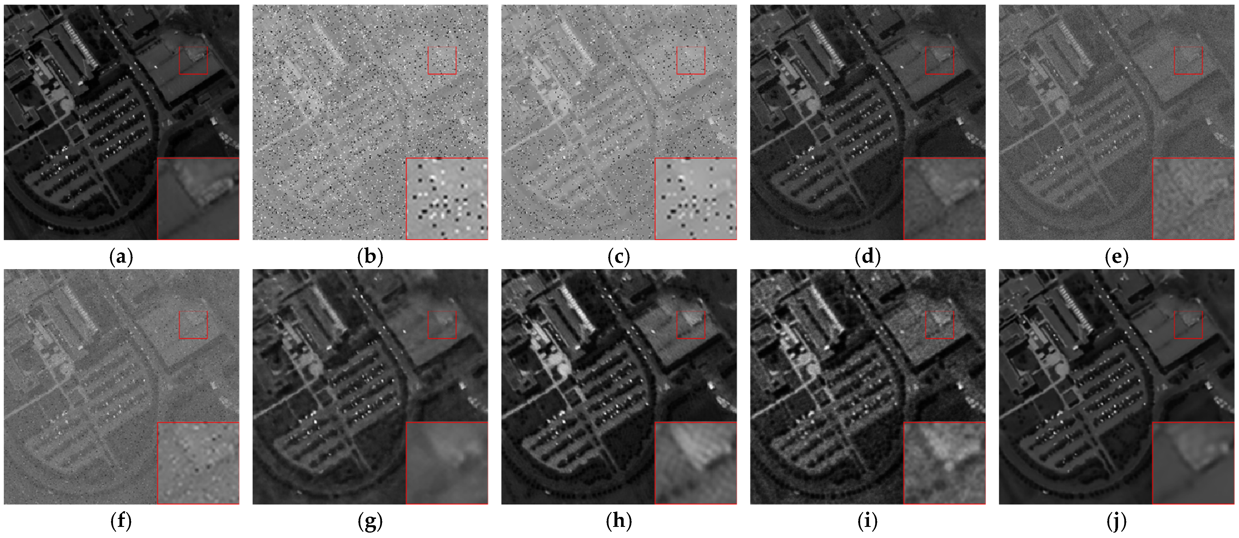
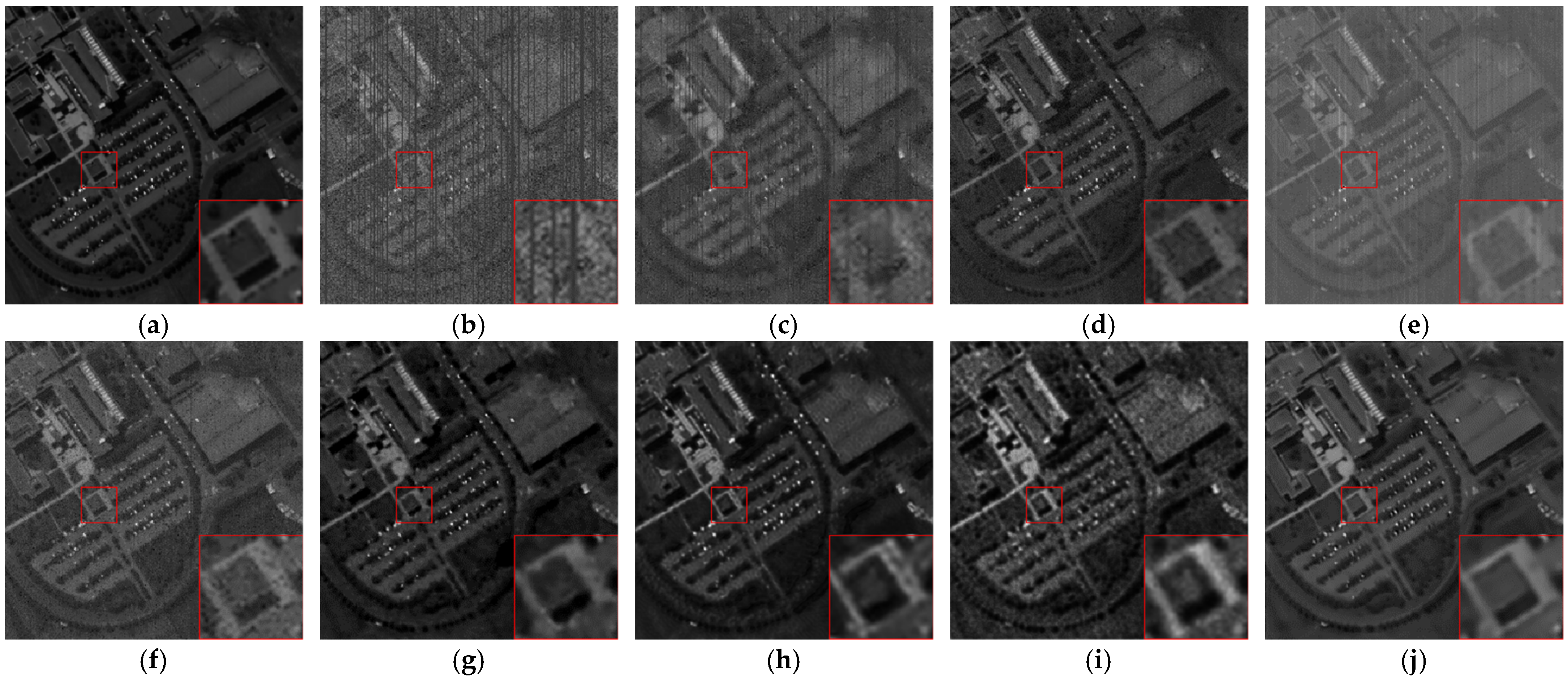
To assess the denoising performance of each algorithm more intuitively, as shown in Figure 5, Figure 6 and Figure 7, we selected the denoising results for Cases 12, 3, and 4 to demonstrate the denoising ability of each algorithm with respect to Gaussian noise and mixed noise.
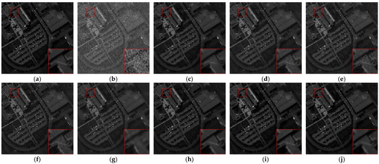
Figure 5.
Case 12—Denoising results of different algorithms in band 7: (a) clean band; (b) noisy band; (c) BM4D; (d) LRMR; (e) HyRes; (f) L1HyMixDe; (g) DHP-2D; (h) SIP; (i) SURE-CNN; and (j) 3S-HSID.
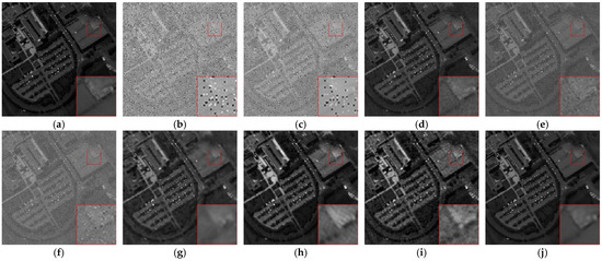
Figure 6.
Case 3—Denoising results of different algorithms in band 26: (a) clean band; (b) noisy band; (c) BM4D; (d) LRMR; (e) HyRes; (f) L1HyMixDe; (g) DHP-2D; (h) SIP; (i) SURE-CNN; and (j) 3S-HSID.
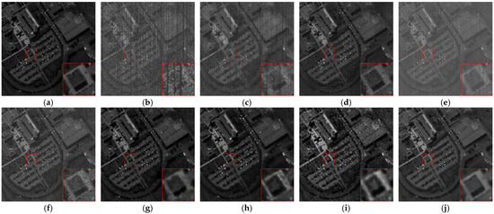
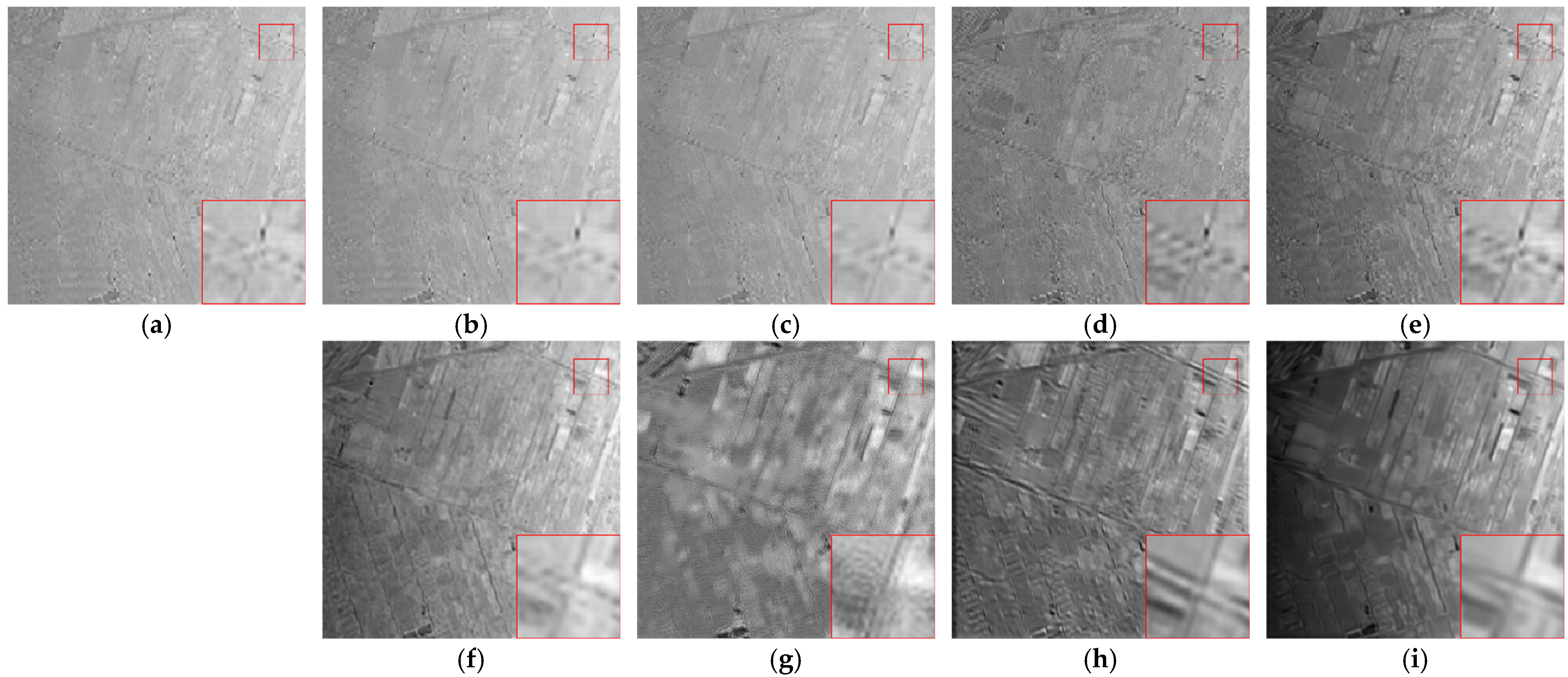
Figure 7.
Case 4—Denoising results of different algorithms in band 19: (a) clean band; (b) noisy band; (c) BM4D; (d) LRMR; (e) HyRes; (f) L1HyMixDe; (g) DHP-2D; (h) SIP; (i) SURE-CNN; and (j) 3S-HSID.
It can be seen, from Figure 5, that BM4D removed the Gaussian noise, but there was a serious loss of information for ground objects with small spatial size, and the image clarity was reduced, such as the road in the red box. LRMR, HyRes, and L1HyMixDe did not completely remove the Gaussian noise. DHP-2D removed the Gaussian noise, but its use resulted in the loss of some ground information and reduced the image clarity. SURE-CNN and SIP removed the Gaussian noise but lost some ground information. Considering the removal of Gaussian noise, 3S-HSID showed better retention of image details, which was also due to the global spectral constraints of 3S-HSID.
It can be seen from Figure 6 that BM4D only dealt with partial Gaussian noise; the removal effect of the salt and pepper noise was poor, and the recovery effect was not ideal. DHP-2D removed the salt and pepper noise from the image but caused a serious loss of image information. HyRes and L1HyMixDe removed most of the salt and pepper noise, but there was still a lot of residual noise in the whole image, which seriously affects the applicability of the image. LRMR, SIP, and SURE-CNN removed the salt and pepper noise, but there was still a lot of residual noise in the image. The 3S-HSID framework removed both the salt and pepper and Gaussian noise from the image. Although some details were lost, the image contour and clarity were better, as shown in the red box.
It can be seen from the noise image in Figure 7 that the original band was affected by Gaussian noise, salt and pepper noise, and bad lines to varying degrees. BM4D did not remove the bad lines from the image, and the denoising results were quite different from the original clean image, as shown in the red box. Although the bad lines in the image were removed by SURE-CNN, SIP, and DHP-2D, the restoration of image details was insufficient, which resulted in a decline in image quality. LRMR, HyRes, and L1HyMixDe did not eliminate the mixed noise, and there was a lot of residual noise. From the perspective of the visual effect, compared with other algorithms, denoising by 3S-HSID has the best effect on mixed noise with an adequate effect on the strip noise existing in the original image.
The denoising performance of the various algorithms cannot be fully evaluated from a single-band visualization analysis. Thus, we also analyzed the denoising results from different aspects, as shown in Figure 8, Figure 9, Figure 10 and Figure 11.
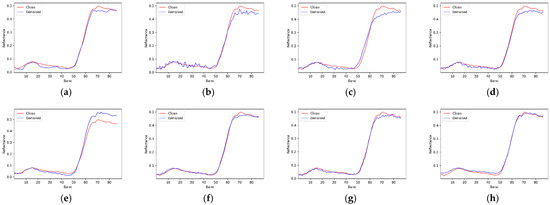
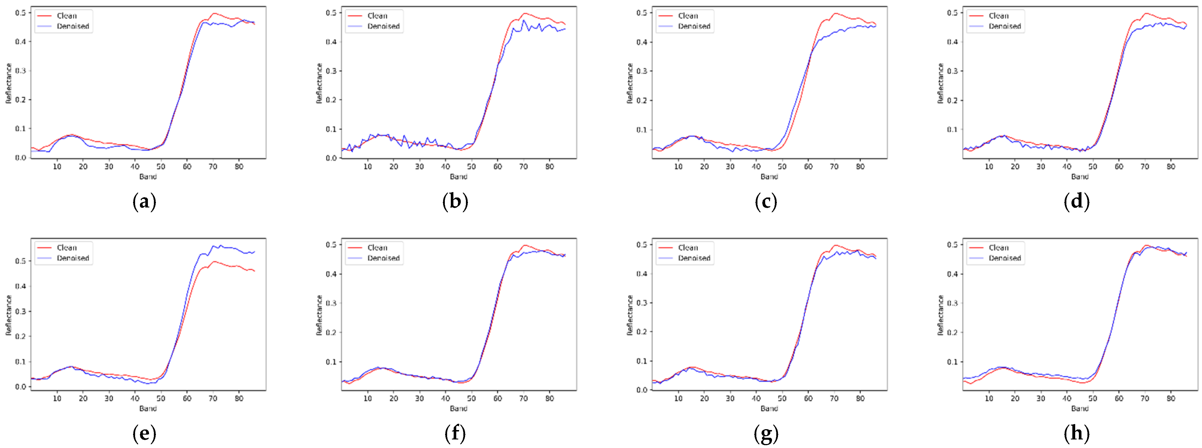
Figure 8.
Recovery of spectral features by different denoising algorithms: (a) BM4D; (b) LRMR; (c) HyRes; (d) L1HyMixDe; (e) DHP-2D; (f) SIP; (g) SURE-CNN; and (h) 3S-HSID.
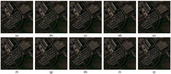
Figure 9.
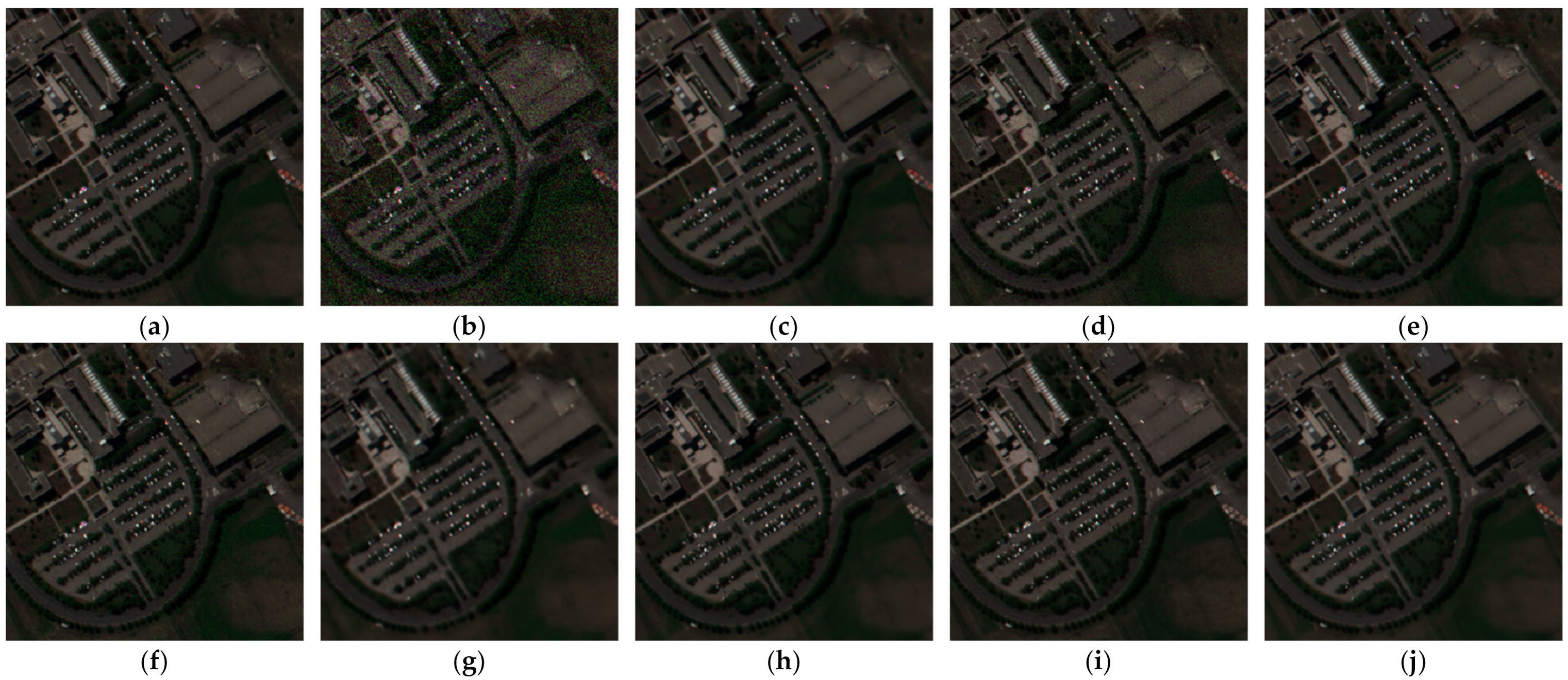
Case 2—Denoising results of different algorithms in RGB (45,15,5): (a) clean image; (b) noisy band; (c) BM4D; (d) LRMR; (e) HyRes; (f) L1HyMixDe; (g) DHP-2D; (h) SIP; (i) SURE-CNN; and (j) 3S-HSID.

Figure 10.
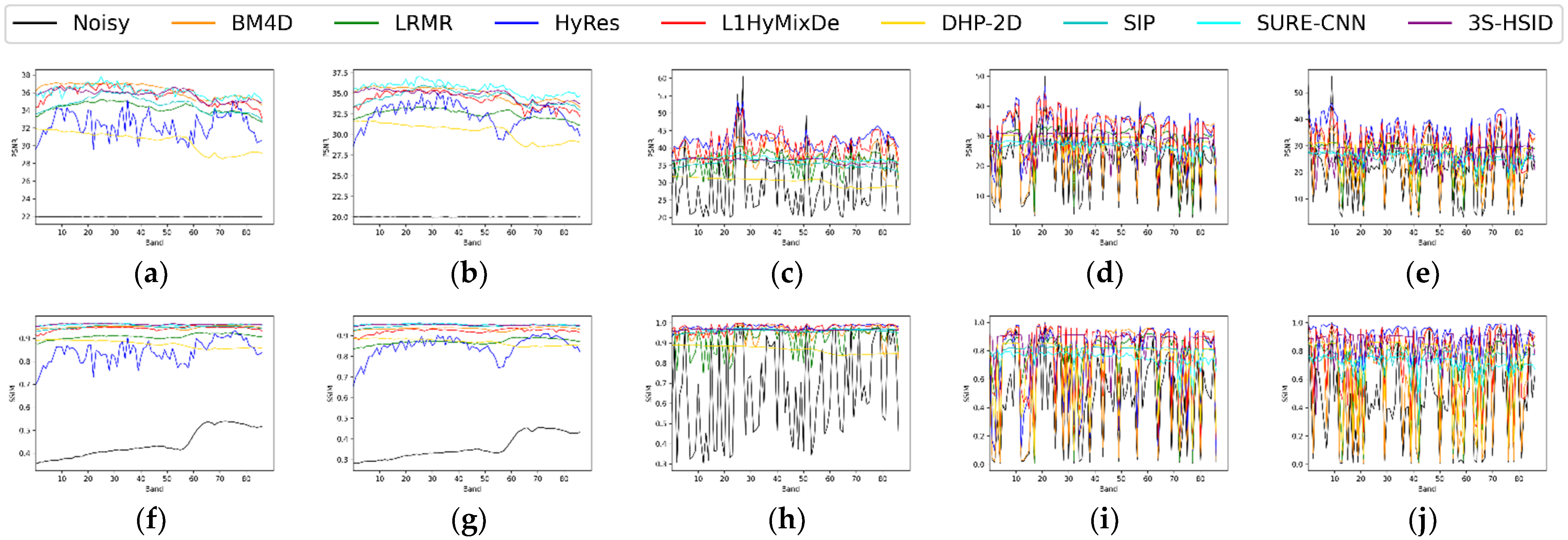
PSNR and SSIM values of different bands: (a) PSNR values of Case 11; (b) PSNR values of Case 12; (c) PSNR values of Case 2; (d) PSNR values of Case 3; (e) PSNR values of Case 4; (f) SSIM values of Case 11; (g) SSIM values of Case 12; (h) SSIM values of Case 2; (i) SSIM values of Case 3; and (j) SSIM values of Case 4.

Figure 11.
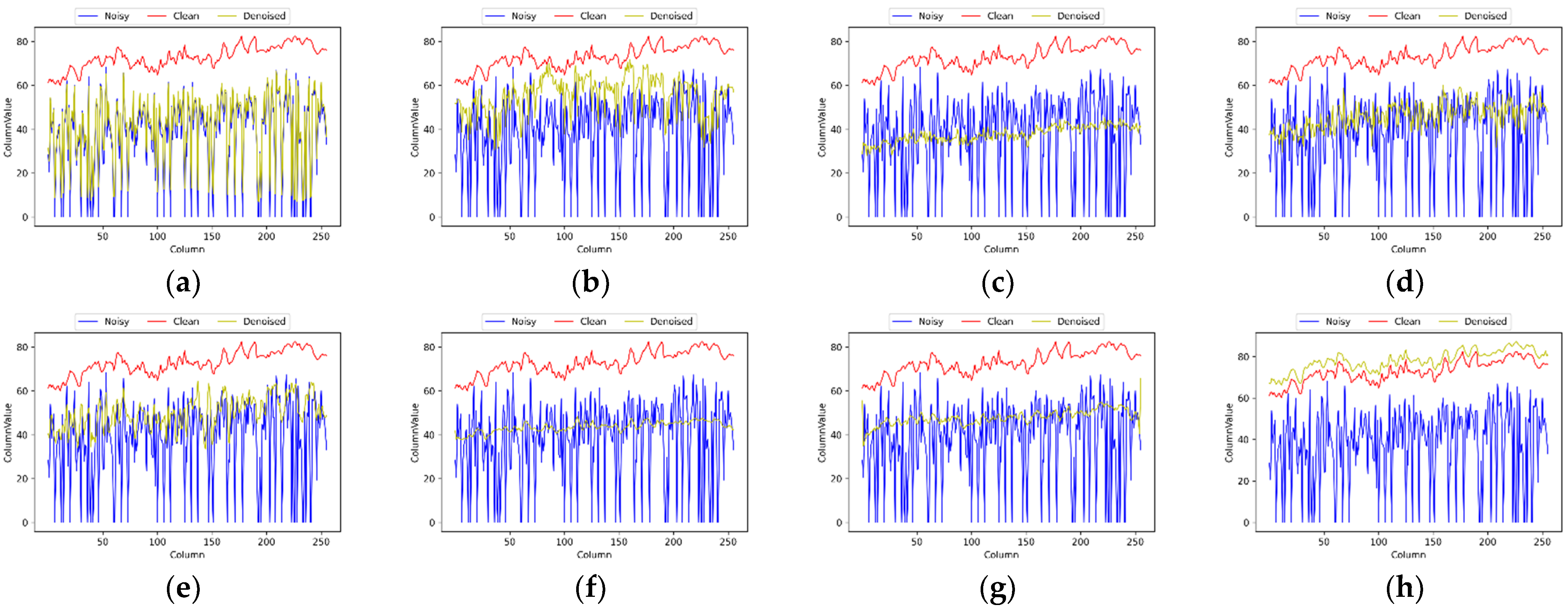
Recovery of bad lines by different denoising algorithms in band 83: (a) BM4D; (b) LRMR; (c) HyRes; (d) L1HyMixDe; (e) DHP-2D; (f) SIP; (g) SURE-CNN; and (h) 3S-HSID.
In Figure 8, we chose the simulated data case11 to extract the spectral curve of one pixel in the image (row = 220, column = 113) and analyzed the spectral recovery performance of each algorithm; the results are shown in Figure 8. From the figure, it can be seen that all of the denoising algorithms adequately restored the spectral characteristics of vegetation’s red-edge, and the spectral characteristics were satisfactorily maintained. However, other algorithms failed to restore the original spectral characteristics in the near-infrared high-reflection region, while 3S-HSID better restored the original spectral details. In the low-reflection region, the self-supervised denoising algorithms SIP, SURE-CNN, and 3S-HSID showed the best recovery effect on the spectral characteristics. Figure 9 shows the denoising results in Case 2. Based on the false-color images, HyRes, L1HyMixDe, and 3S-HSID showed a good performance in color maintenance, especially in the right red roof area.
The PSNR and SSIM values of hyperspectral images were obtained by calculating the PSNR and SSIM values for all bands, and the noise effects in different bands of the hyperspectral images varied. The denoising performance of the denoising algorithms for each band can be more intuitively seen in a band-by-band analysis. The PSNR and SSIM curves for the denoising results of various algorithms in different bands are shown in Figure 10. From the figure, it can be seen that the denoising performance of 3S-HSID was relatively stable in different bands when dealing with images dominated by Gaussian noise, indicating that the algorithm was robust and effective in removing Gaussian noise of different intensities. When dealing with the bands that have strong noise influence, such as salt and pepper noise and bad lines, the advantage of denoising by 3S-HSID was more obvious. In addition, by analyzing the PSNR and SSIM values of each band in the noise images, we found that the PSNR and SSIM values of some bands were very high. This is mainly because, when the noise was simulated, the bands to which the noise was applied were randomly selected, and not all bands had added noise. This led to a very small number of bands being unaffected by any noise, and no bands in the real images were completely clean. This is also the reason why HyRes and L1HyMixDe achieved higher PSNR and SSIM values for some data. By comparing the SAM values of different algorithms, it can be found that other algorithms took into account the denoising effect in the spectral direction while denoising in the spatial direction. From the visualization results, it can also be seen that HyRes and L1HyMixDe are not the best choice for band recovery in images affected by noise.
Mixed noise can be considered the closest case to real image noise, and the influence of bad lines on image quality is especially obvious. We selected the 77th band of Case 4 to analyze the recovery of bad line noise. In Figure 11, the pixel values are displayed in the direction of the band column. It can be seen from the distribution of the blue curve (noise image) that the bad lines had great influence on the quality of the original band. BM4D could not satisfactorily remove the bad lines, and other methods for bad line removal had a certain effect. Although the compared algorithms were able to process mixed noise, the difference between the denoising results and the sum of pixel values in the column direction of the original band was large, as can be seen when comparing the distribution position of the curve, while the difference between the 3S-HSID output and the sum of pixel values in the column direction of the original band was the smallest. The curve characteristics were consistent with those of the sum of pixel values in the column direction of the original band, indicating that 3S-HSID has a good denoising performance for mixed noise.
3.3. Real Satellite HSIs Denoising Experiment
To verify the universality and practicability of 3S-HSID, we conducted denoising experiments using real satellite hyperspectral images. Satellite hyperspectral data from different imaging spectrometers were used, which had varying spatial resolutions, spectral resolutions, and band numbers. As these data are real and have no noise-free reference, we compared the denoising performance of 3S-HSID with other algorithms based on the visual effects of the denoising results, as shown in Figure 12, Figure 13, Figure 14, Figure 15, Figure 16, Figure 17 and Figure 18, which depict the denoising results for the hyperspectral data of different satellite platforms, spatial resolutions, and spectral resolutions.
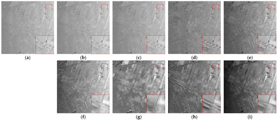
Figure 12.
GF-14 hyperspectral image (SWIR) denoising results with band 1: (a) real image; (b) BM4D; (c) LRMR; (d) HyRes; (e) L1HyMixDe; (f) DHP-2D; (g) SIP; (h) SURE-CNN; and (i) 3S-HSID.
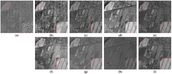
Figure 13.
GF-14 hyperspectral image (VNIR) denoising results with band 5: (a) real image; (b) BM4D; (c) LRMR; (d) HyRes; (e) L1HyMixDe; (f) DHP-2D; (g) SIP; (h) SURE-CNN; and (i) 3S-HSID.

Figure 14.
GF-14 hyperspectral image (VNIR) denoising results with false-color image (R: band 40, G: band 15, B: band 5): (a) real image; (b) BM4D; (c) LRMR; (d) HyRes; (e) L1HyMixDe; (f) DHP-2D; (g) SIP; (h) SURE-CNN; and (i) 3S-HSID.
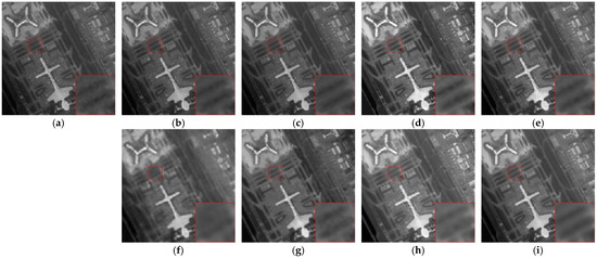
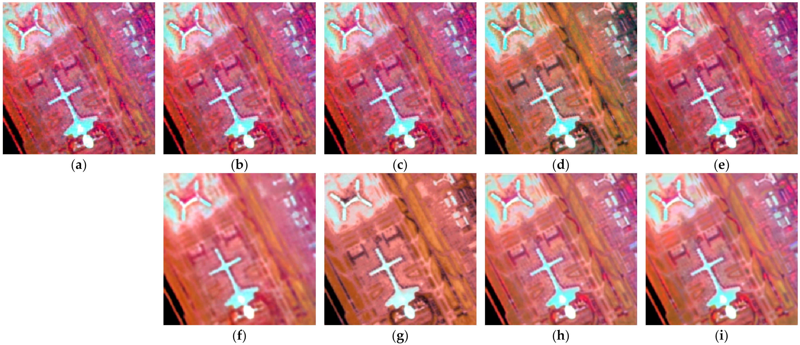
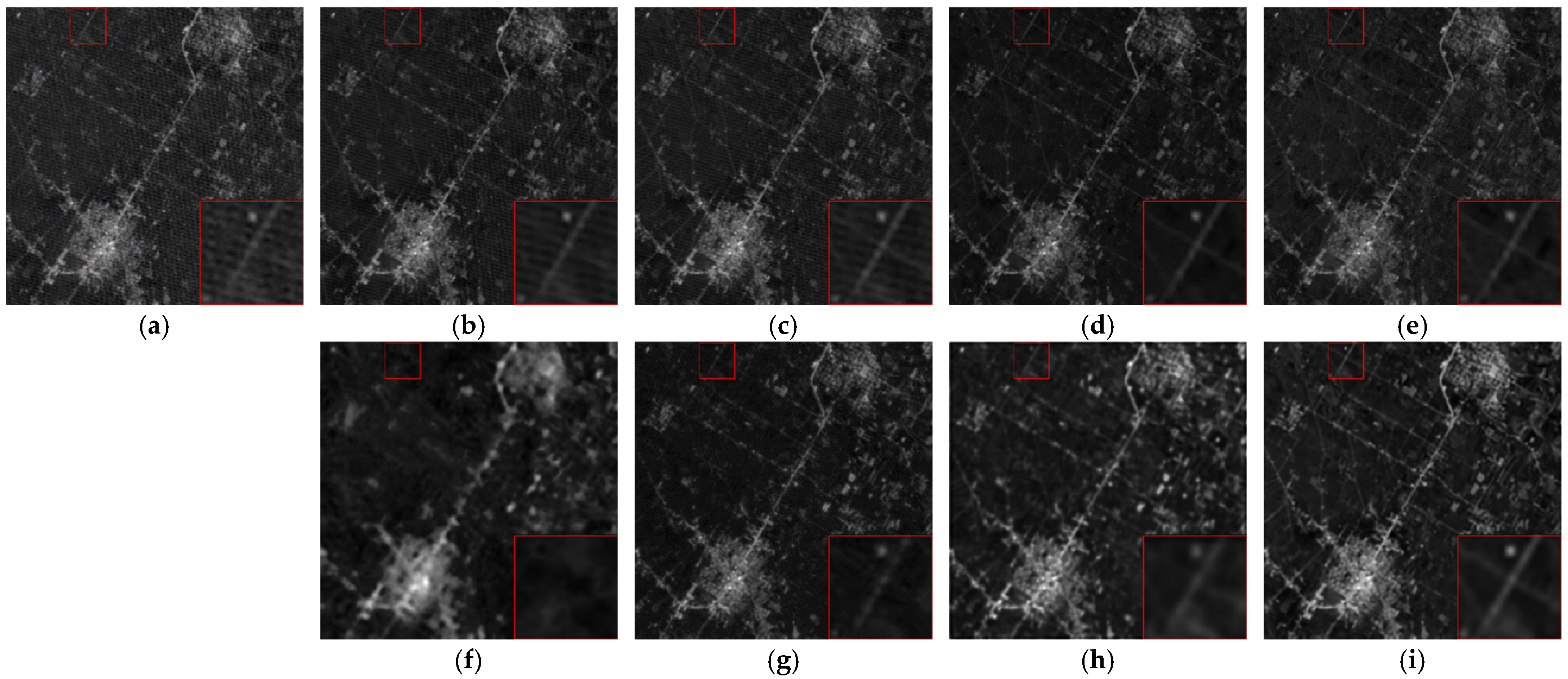
Figure 15.
ZH-1 hyperspectral image denoising results with band 1: (a) real image; (b) BM4D; (c) LRMR; (d) HyRes; (e) L1HyMixDe; (f) DHP-2D; (g) SIP; (h) SURE-CNN; and (i) 3S-HSID.

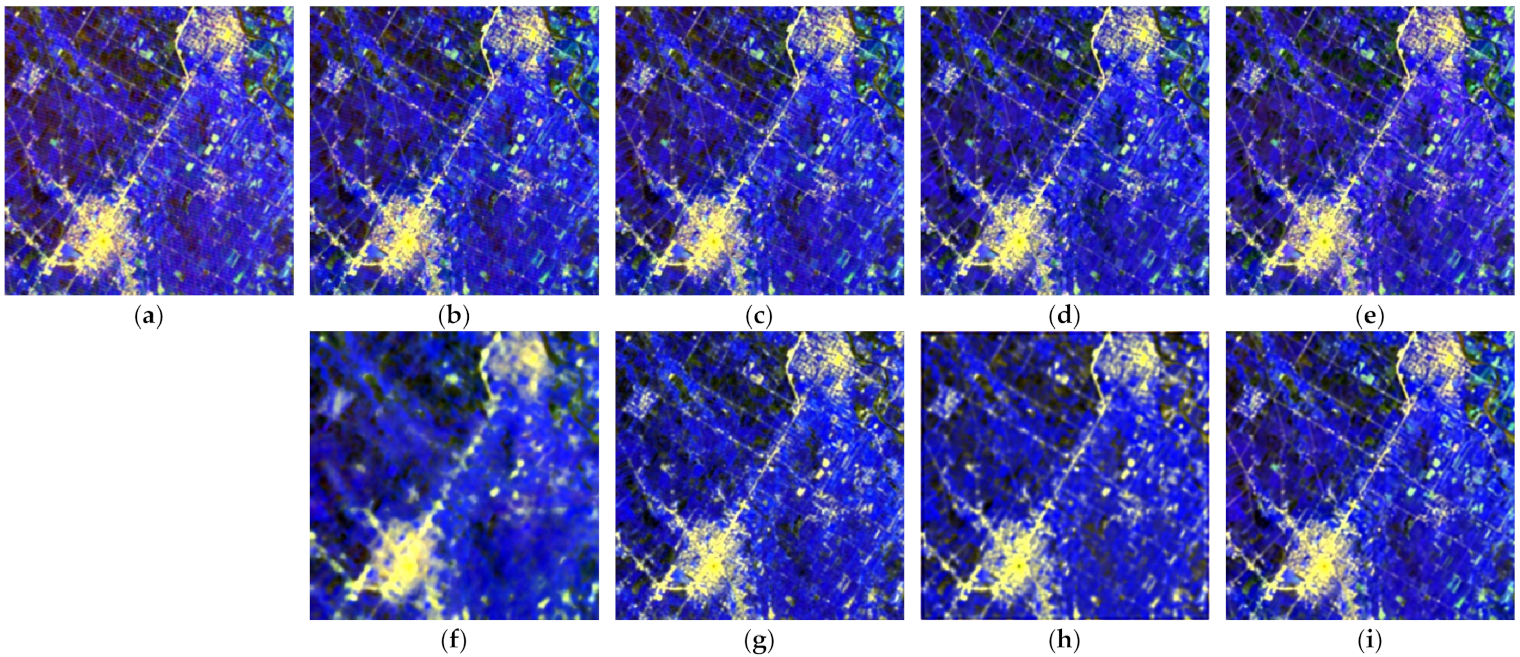
Figure 16.
ZH-1 hyperspectral image denoising results with false-color image (R: band 32, G: band 20, B: band 1): (a) real image; (b) BM4D; (c) LRMR; (d) HyRes; (e) L1HyMixDe; (f) DHP-2D; (g) SIP; (h) SURE-CNN; and (i) 3S-HSID.
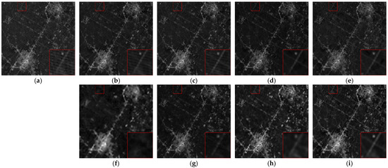
Figure 17.
PRISMA hyperspectral image denoising results with band 66: (a) real image; (b) BM4D; (c) LRMR; (d) HyRes; (e) L1HyMixDe; (f) DHP-2D; (g) SIP; (h) SURE-CNN; and (i) 3S-HSID.

Figure 18.
PRISMA hyperspectral image denoising results with false-color image (R: band 66, G: band 40, B: band 1): (a) real image; (b) BM4D; (c) LRMR; (d) HyRes; (e) L1HyMixDe; (f) DHP-2D; (g) SIP; (h) SURE-CNN; and (i) 3S-HSID.
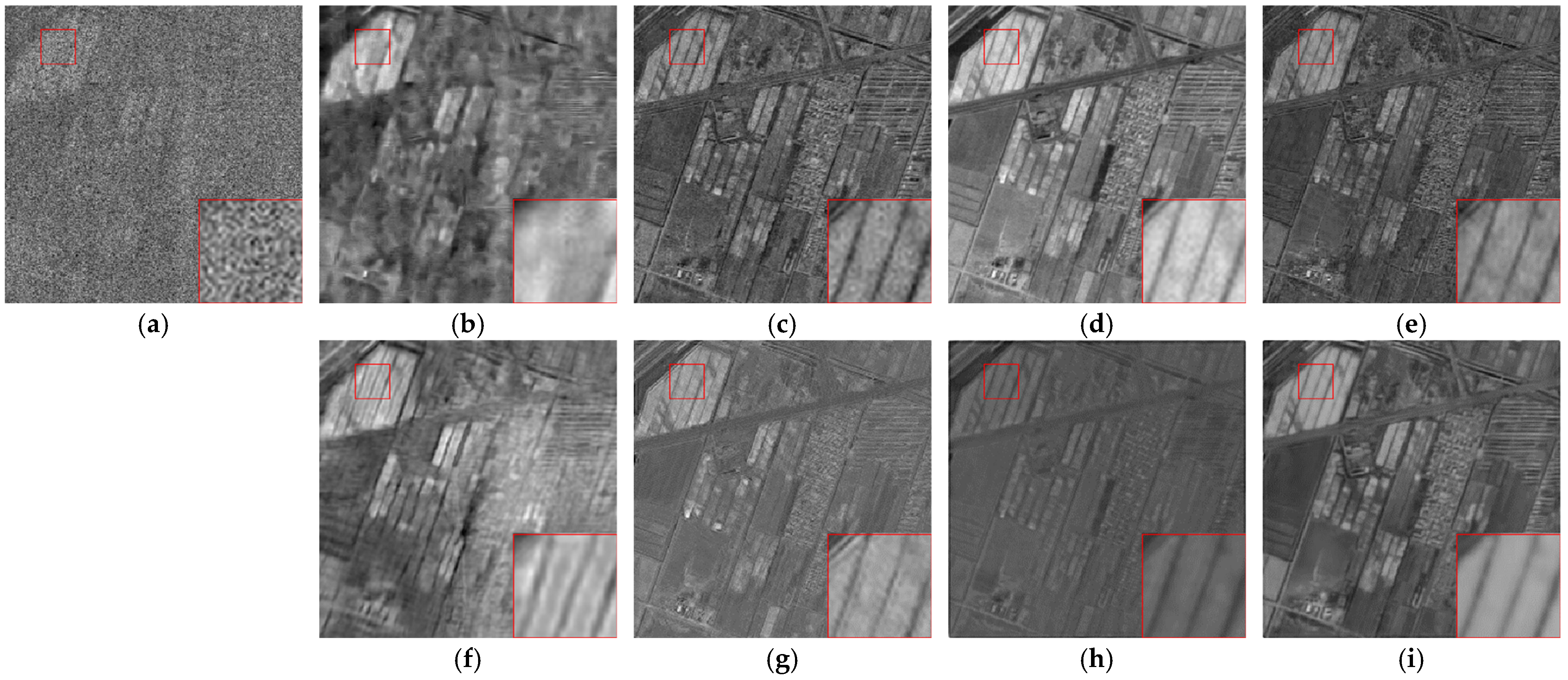
The band seen in Figure 12 appeared to be affected by Gaussian noise, especially in the upper left corner region. The noise processing effect of BM4D and the model-based methods was not obvious. The noise processing effect of the self-supervised learning denoising algorithms, such as SIP, was not ideal, and the image quality of the denoising results was not high. The 3S-HSID framework could better recover the image and show the image details, as shown in the red box, due to the fact that our algorithm can simultaneously retrieve all bands for processing.
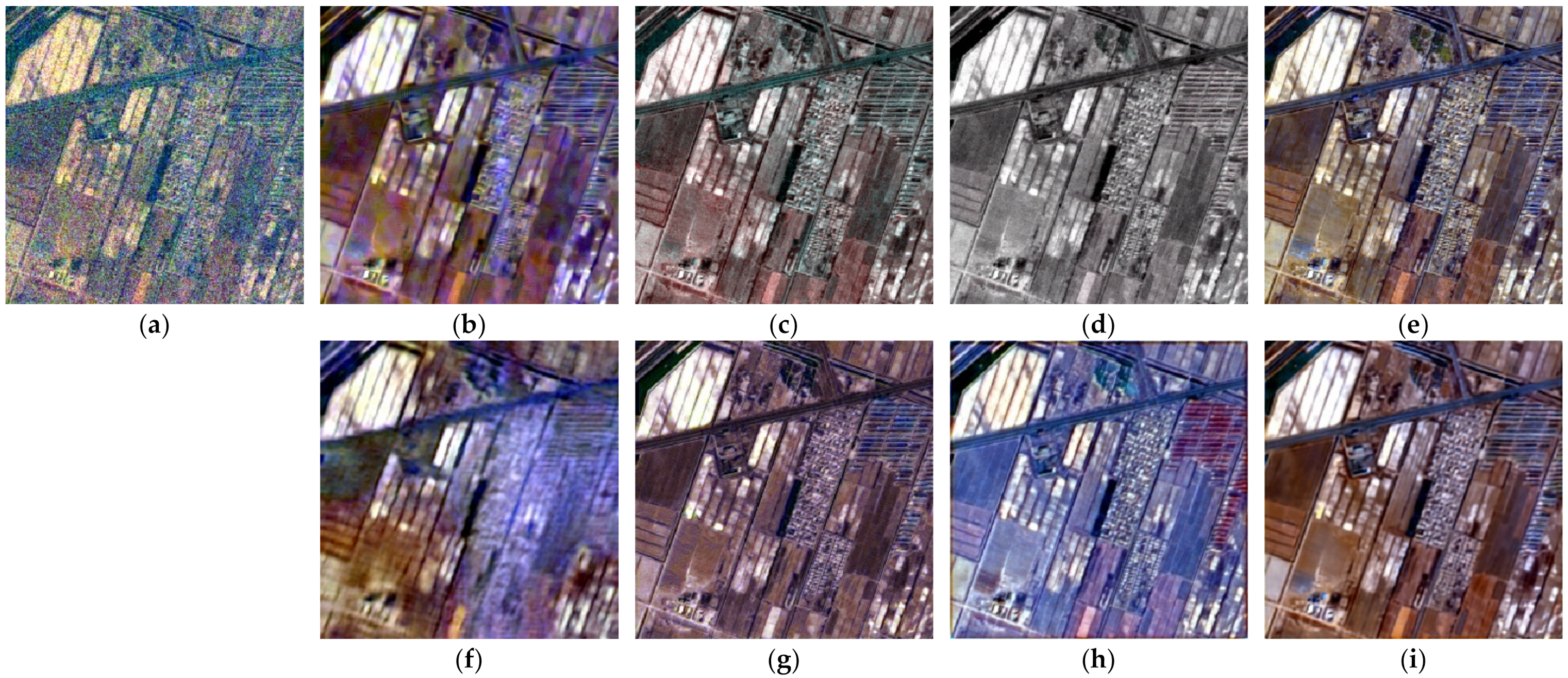
Similar to SWIR images, VNIR images are typically seriously affected by Gaussian noise. It can be seen from Figure 13 that BM4D and DHP-2D were not ideal for image restoration in this case. The result of HyRes is better in noise removal for a single band, but its performance is not good for all the bands, such as tone distortion, as shown in Figure 14d. L1HyMixDe and 3S-HSID performed better than the other algorithms in image restoration, especially regarding the restoration of farmland and housing texture details. As shown in the red boxes, the effect of 3S-HSID on farmland boundary restoration is very clear.
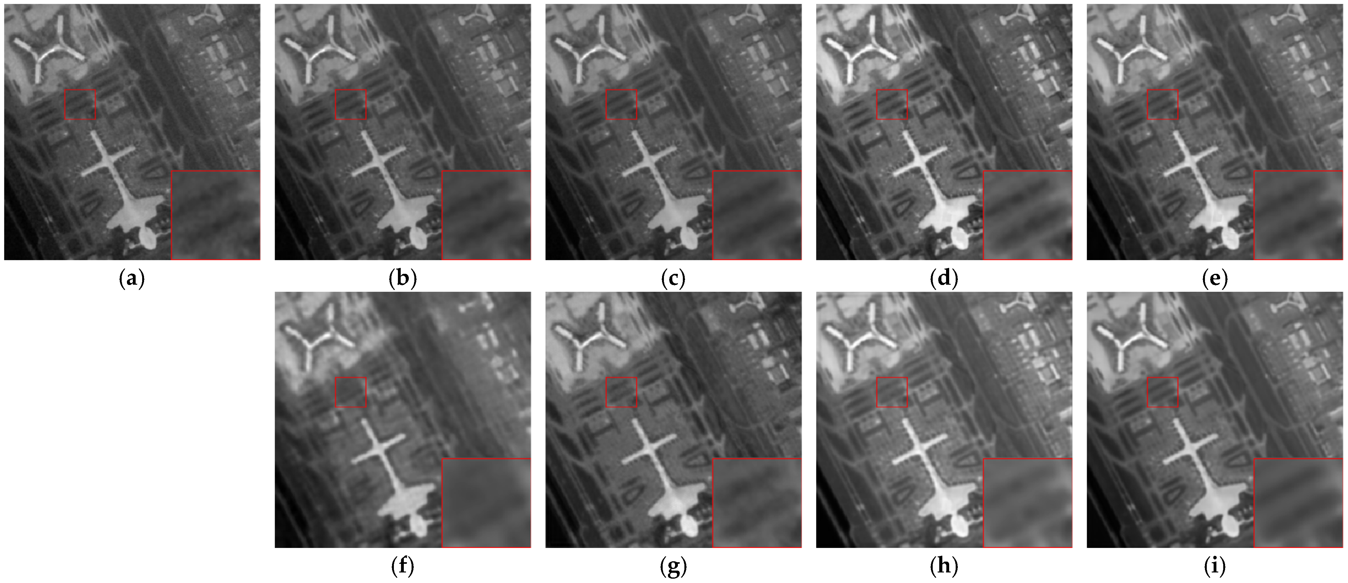
It can be seen from Figure 15a that the single band was only slightly affected by noise, which had little effect on the image details. Therefore, all of the compared algorithms could recover the image to some extent. The recovery effect of DHP-2D was relatively poor, as the recovery of image details was not ideal. The false color images show that the noise intensity of different bands is different, as presented in Figure 16. The model-based methods have a certain removal effect on mixed noise, but there are blur and tone distortions. The 3S-HSID framework deals with noise in the airport runway, terminal, and other areas, and the image details were clearer, as shown in the red box.
As presented in Figure 17a and Figure 18a, the original images had very serious stripe noise, and neither BM4D nor the model-based methods could completely remove the stripe noise from the image. Although DHP-2D, SIP, and SURE-CNN displayed certain suppression of the stripe noise, they were not ideal in terms of maintaining image details, as shown in Figure 18f,h. In contrast, 3S-HSID effectively removed the mixed noise in the image, especially the stripe noise. Although the spatial resolution of PRISMA satellite hyperspectral image is low, 3S-HSID still restored the image details well.
4. Discussion
4.1. Hyperparametric Analysis
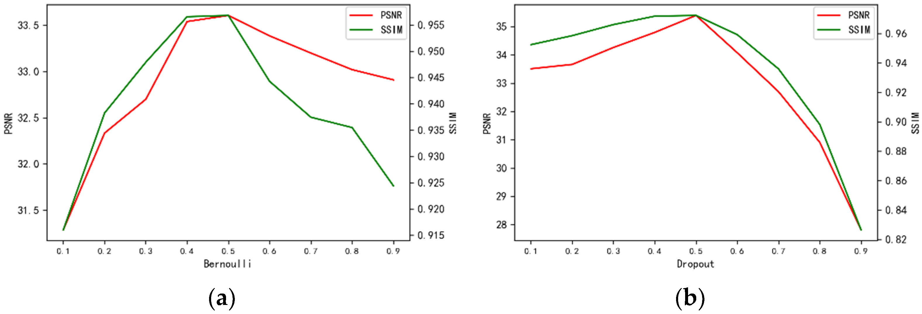
- Bernoulli sampling probability and dropout probability
In this experiment, the Bernoulli sampling probability b and dropout probability p are some of the most important hyperparameters. We used Case11 simulation data to test the selection of these two probability values. In the experiment, the dropout probability was , and the Bernoulli sampling probability was , with an interval of 0.1. In the form of cross-validation, the dropout probability and Bernoulli sampling probability were added to the experiment. After the experiment was completed, the PSNR values of all denoising results were calculated. To find the optimal combination, we fixed a certain probability value and calculated the average PSNR value of all denoising results in the range of under the current probability value, as shown in Figure 19. From the experimental results, it can be seen that 3S-HSID demonstrated the best denoising performance when and .
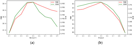
Figure 19.
The (a) Bernoulli sampling and (b) dropout probability hyperparameters.
- Number of iterations
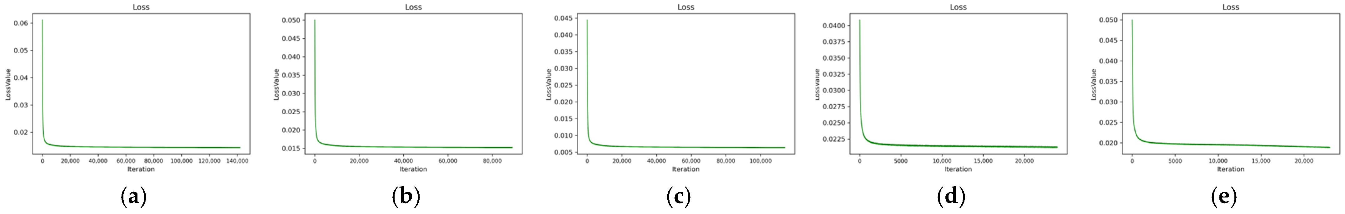
In the 3S-HSID training process, the number of iterations is one of the factors affecting the denoising effect. However, as the model converges, it is no longer the case that the denoising effect of the model is higher, given a higher number of iterations. Therefore, we set the termination condition of iteration and determined whether to stop training according to whether the optimal denoising model was obtained. The termination condition of training was to stop training without updating the current optimal denoising results after 8000 rounds of continuous training. According to the previous analysis, the final denoising result was obtained by averaging the multiple denoising results, and the PSNR values of the denoising results were obtained by calculating the different average times. Therefore, judgment of whether the denoising effect is optimal was based on the continuous increase in average time, up to the point when the PSNR value of the current optimal denoising result is no longer updated. Based on this, 3S-HSID can adaptively end the training process and obtain the optimal denoising results, thus avoiding model overfitting. In the denoising experiment using simulated data, the curve for the relationship between the loss function and the number of iterations is shown in Figure 20. It can be seen from the figure that the loss function value decreases rapidly. With an increase in the number of iterations, the network model is continuously refined to obtain the optimal denoising results. Thanks to the dropout strategy, the phenomenon of model overfitting does not appear with the increase in iterations. We determined the iteration training number for real satellite hyperspectral data according to the iteration number obtained in the simulated hyperspectral data denoising experiment. The optimal number of iterations for satellite hyperspectral image data on different platforms was determined to be 30,000. From the experimental results, the mixed noise in the image could be effectively removed in different bands, indicating that this number of iterations is reasonable and effective.
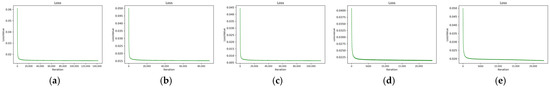
Figure 20.
Relationship between loss value and the number of iterations for: (a) Case 11, iterations = 142,000; (b) Case 12, iterations = 89,000; (c) Case 2, iterations = 114,000; (d) Case 3, iterations = 24,000; and (e) Case 4, iterations = 23,000.
4.2. Future Works
Although 3S-HSID achieved a good denoising effect in our experiments, the algorithm still needs to be improved for use in practical applications. On one hand, the algorithm only denoises a single hyperspectral image. In the face of massive satellite hyperspectral data, how to carry out batch processing remains to be further studied. On the other hand, 3S-HSID needs to re-learn the noise distribution of hyperspectral images obtained by different satellite hyperspectral imagers. How to achieve the same effect as denoising methods based on supervised learning, such that the generalization of the denoising model can be strengthened, also requires further research.
5. Conclusions
A robust denoising method is crucial for the subsequent processing and application of satellite hyperspectral images. Common denoising methods based on deep learning often require a large number of clean/noisy image pairs as training samples, which are extremely difficult to obtain from real satellite hyperspectral imagery. The use of a single satellite hyperspectral image denoising algorithm based on self-supervised learning can effectively solve this problem. The 3S-HSID framework developed in this paper uses Bernoulli sampling to skillfully construct the clean/noisy image pairs required for training and uses a random discard strategy during training and testing to prevent the overfitting problem caused by insufficient samples. At the same time, 3S-HSID uses partial convolution to help restore noise-contaminated pixels. For the model loss function, we proposed a local loss function based on mean variance and a global loss function based on spectral consistency, which effectively preserve the spatial and spectral domain features before and after denoising. Based on the Pavia University dataset, we simulated the influences of Gaussian noise, salt and pepper noise, bad lines, and mixed noise on hyperspectral data. It was found that 3S-HSID can achieve a better denoising effect than most of the state-of-the-art traditional and unsupervised/self-supervised methods. Note that the spectral characteristics are well preserved. In the mixed noise removal experiment, the spectral similarity between the 3S-HSID denoising result and original data is 0.2055; compared with traditional methods and model-based methods, the improvement is obvious. At the same time, we used real satellite hyperspectral images with different sensors, spatial resolutions, and spectral resolutions to test the effect of denoising using 3S-HSID. The denoising results on GF-14, ZH-1, and PRISMA datasets demonstrated the reliability and universality of the proposed algorithm. Data preprocessing plays an important role in hyperspectral satellite ground processing systems. The excellent denoising performance of 3S-HSID provides a new technical means for real satellite hyperspectral image denoising. We recognize that 3S-HSID still has shortcomings. On the one hand, 3S-HSID denoises all bands at one time, due to a large number of hyperspectral data bands; the time consumption of 3S-HSID is longer than that of other algorithms. On the other hand, the U-shaped structure of the U-Net network will lead to a certain degree of spatial information loss, which is reflected in the PSNR measurement.
Author Contributions
Conceptualization, J.Q., H.Z. and B.L.; methodology, J.Q.; software, J.Q.; validation, J.Q. and H.Z.; formal analysis, J.Q. and H.Z.; investigation, J.Q.; resources, H.Z.; data curation, J.Q.; writing—original draft preparation, J.Q.; writing—review and editing, J.Q. and H.Z.; visualization, J.Q.; supervision, H.Z.; project administration, H.Z.; funding acquisition, H.Z. All authors have read and agreed to the published version of the manuscript.
Funding
This research was funded by the National Natural Science Foundation of China under Grant 41971379.
Data Availability Statement
Pavia university dataset: http://www.ehu.eus/ccwintco/index.php?title=Hyperspectral_Remote_Sensing_Scenes; PRISMA dataset: http://prisma.asi.it/missionselect/; other datasets: https://cloud.tsinghua.edu.cn/f/f1883b2d6b8f43dd898c/?dl=1. All data can be accessed on 23 June 2022.
Conflicts of Interest
The authors declare no conflict of interest.
References
- Transon, J.; D’Andrimont, R.; Maugnard, A.; Defourny, P. Survey of Hyperspectral Earth Observation Applications from Space in the Sentinel-2 Context. Remote Sens. 2018, 10, 157. [Google Scholar] [CrossRef] [Green Version]
- Meng, S.; Wang, X.; Hu, X.; Luo, C.; Zhong, Y. Deep learning-based crop mapping in the cloudy season using one-shot hyperspectral satellite imagery. Comput. Electron. Agric. 2021, 186, 106188. [Google Scholar] [CrossRef]
- Pandey, D.; Tiwari, K.C. New spectral indices for detection of urban built-up surfaces and its sub-classes in AVIRIS-NG hyperspectral imagery. Geocarto Int. 2020, 37, 1949–1970. [Google Scholar] [CrossRef]
- Niroumand-Jadidi, M.; Bovolo, F.; Bruzzone, L. Water Quality Retrieval from PRISMA Hyperspectral Images: First Experience in a Turbid Lake and Comparison with Sentinel-2. Remote Sens. 2020, 12, 3984. [Google Scholar] [CrossRef]
- Xie, Y.; Sha, Z.; Mesev, V. Remote Sensing of Sustainable Ecosystems. J. Sens. 2018, 2018, 9683415. [Google Scholar] [CrossRef]
- Chen, Y.; Cao, X.; Zhao, Q.; Meng, D.; Xu, Z. Denoising Hyperspectral Image with Non-i.i.d. Noise Structure. IEEE Trans. Cybern. 2018, 48, 1054–1066. [Google Scholar] [CrossRef] [PubMed] [Green Version]
- Nalepa, J.; Myller, M.; Cwiek, M.; Zak, L.; Lakota, T.; Tulczyjew, L.; Kawulok, M. Towards On-Board Hyperspectral Satellite Image Segmentation: Understanding Robustness of Deep Learning through Simulating Acquisition Conditions. Remote Sens. 2021, 13, 1532. [Google Scholar] [CrossRef]
- He, W.; Zhang, H.; Zhang, L.; Shen, H. Total-Variation-Regularized Low-Rank Matrix Factorization for Hyperspectral Image Restoration. IEEE Trans. Geosci. Remote Sens. 2016, 54, 178–188. [Google Scholar] [CrossRef]
- Dabov, K.; Foi, A.; Katkovnik, V.; Egiazarian, K. Image Denoising by Sparse 3-D Transform-Domain Collaborative Filtering. IEEE Trans. Image Processing 2007, 16, 2080–2095. [Google Scholar] [CrossRef]
- Buades, A.; Coll, B.; Morel, J. A non-local algorithm for image denoising. In Proceedings of the 2005 IEEE Computer Society Conference on Computer Vision and Pattern Recognition (CVPR’05), San Diego, CA, USA, 20–25 June 2005; Volume 2, pp. 60–65. [Google Scholar]
- Gu, S.; Zhang, L.; Zuo, W.; Feng, X. Weighted Nuclear Norm Minimization with Application to Image Denoising. In Proceedings of the 2014 IEEE Conference on Computer Vision and Pattern Recognition, Columbus, OH, USA, 23–28 June 2014; pp. 2862–2869. [Google Scholar]
- Xie, W.; Li, Y.; Jia, X. Deep convolutional networks with residual learning for accurate spectral-spatial denoising. Neurocomputing 2018, 312, 372–381. [Google Scholar] [CrossRef]
- Zhang, H.; He, W.; Zhang, L.; Shen, H.; Yuan, Q. Hyperspectral Image Restoration Using Low-Rank Matrix Recovery. IEEE Trans. Geosci. Remote Sens. 2014, 52, 4729–4743. [Google Scholar] [CrossRef]
- Rasti, B.; Ulfarsson, M.O.; Ghamisi, P. Automatic Hyperspectral Image Restoration Using Sparse and Low-Rank Modeling. IEEE Geosci. Remote Sens. Lett. 2017, 14, 2335–2339. [Google Scholar] [CrossRef]
- Xue, J.; Zhao, Y.; Liao, W.; Kong, S. Joint Spatial and Spectral Low-Rank Regularization for Hyperspectral Image Denoising. IEEE Trans. Geosci. Remote Sens. 2017, 56, 1940–1958. [Google Scholar] [CrossRef]
- Xue, J.; Zhao, Y.; Liao, W.; Chan, J.C. Nonlocal Low-Rank Regularized Tensor Decomposition for Hyperspectral Image Denoising. IEEE Trans. Geosci. Remote Sens. 2019, 57, 5174–5189. [Google Scholar] [CrossRef]
- Yuan, Q.; Zhang, L.; Shen, H. Hyperspectral Image Denoising Employing a Spectral–Spatial Adaptive Total Variation Model. IEEE Trans. Geosci. Remote Sens. 2012, 50, 3660–3677. [Google Scholar] [CrossRef]
- Aggarwal, H.K.; Majumdar, A. Hyperspectral Image Denoising Using Spatio-Spectral Total Variation. IEEE Geosci. Remote Sens. Lett. 2016, 13, 442–446. [Google Scholar] [CrossRef]
- Li, J.; Yuan, Q.; Shen, H.; Zhang, L. Noise Removal From Hyperspectral Image With Joint Spectral–Spatial Distributed Sparse Representation. IEEE Trans. Geosci. Remote Sens. 2016, 54, 5425–5439. [Google Scholar] [CrossRef]
- Lu, T.; Li, S.; Fang, L.; Ma, Y.; Benediktsson, J.A. Spectral–Spatial Adaptive Sparse Representation for Hyperspectral Image Denoising. IEEE Trans. Geosci. Remote Sens. 2016, 54, 373–385. [Google Scholar] [CrossRef]
- Candès, E.J.; Li, X.; Ma, Y.; Wright, J. Robust principal component analysis? J. ACM 2011, 58, 1–37. [Google Scholar] [CrossRef]
- Lefkimmiatis, S.; Roussos, A.; Maragos, P.; Unser, M. Structure Tensor Total Variation. SIAM J. Imaging Sci. 2015, 8, 1090–1122. [Google Scholar] [CrossRef]
- Fei, X.; Miao, J.; Zhao, Y.; Huang, W.; Yu, R. Total Variation Regularized Low-Rank Model With Directional Information for Hyperspectral Image Restoration. IEEE Access 2021, 9, 84156–84169. [Google Scholar] [CrossRef]
- Xie, W.; Li, Y. Hyperspectral Imagery Denoising by Deep Learning With Trainable Nonlinearity Function. IEEE Geosci. Remote Sens. Lett. 2017, 14, 1963–1967. [Google Scholar] [CrossRef]
- Zhang, K.; Zuo, W.; Chen, Y.; Meng, D.; Zhang, L. Beyond a Gaussian Denoiser: Residual Learning of Deep CNN for Image Denoising. IEEE Trans. Image Processing 2017, 26, 3142–3155. [Google Scholar] [CrossRef] [PubMed] [Green Version]
- Xie, W.; Li, Y.; Hu, J.; Chen, D.-Y. Trainable spectral difference learning with spatial starting for hyperspectral image denoising. Neural Netw. 2018, 108, 272–286. [Google Scholar] [CrossRef]
- Yuan, Q.; Zhang, Q.; Li, J.; Shen, H.; Zhang, L. Hyperspectral Image Denoising Employing a Spatial–Spectral Deep Residual Convolutional Neural Network. IEEE Trans. Geosci. Remote Sens. 2019, 57, 1205–1218. [Google Scholar] [CrossRef] [Green Version]
- Maffei, A.; Haut, J.M.; Paoletti, M.E.; Plaza, J.; Bruzzone, L.; Plaza, A. A Single Model CNN for Hyperspectral Image Denoising. IEEE Trans. Geosci. Remote Sens. 2020, 58, 2516–2529. [Google Scholar] [CrossRef]
- Liu, S.; Feng, J.; Tian, Z. Variational Low-Rank Matrix Factorization with Multi-Patch Collaborative Learning for Hyperspectral Imagery Mixed Denoising. Remote Sens. 2021, 13, 1101. [Google Scholar] [CrossRef]
- Zhuang, L.; Ng, M.K.; Fu, X. Hyperspectral Image Mixed Noise Removal Using Subspace Representation and Deep CNN Image Prior. Remote Sens. 2021, 13, 4098. [Google Scholar] [CrossRef]
- Jiang, T.X.; Zhuang, L.; Huang, T.Z.; Zhao, X.L.; Bioucas-Dias, J.M. Adaptive Hyperspectral Mixed Noise Removal. IEEE Trans. Geosci. Remote Sens. 2022, 60, 1–13. [Google Scholar] [CrossRef]
- Xiong, F.; Zhou, J.; Zhao, Q.; Lu, J.; Qian, Y. MAC-Net: Model-Aided Nonlocal Neural Network for Hyperspectral Image Denoising. IEEE Trans. Geosci. Remote Sens. 2022, 60, 1–14. [Google Scholar] [CrossRef]
- Kan, Z.; Li, S.; Zhang, Y. Attention-Based Octave Dense Network for Hyperspectral Image Denoising. In Proceedings of the 2021 IEEE 4th International Conference on Big Data and Artificial Intelligence (BDAI), Qingdao, China, 2–4 July 2021; pp. 230–235. [Google Scholar]
- Shi, Q.; Tang, X.; Yang, T.; Liu, R.; Zhang, L. Hyperspectral Image Denoising Using a 3-D Attention Denoising Network. IEEE Trans. Geosci. Remote Sens. 2021, 59, 10348–10363. [Google Scholar] [CrossRef]
- Wang, Z.; Shao, Z.; Huang, X.; Wang, J.; Lu, T. SSCAN: A Spatial–Spectral Cross Attention Network for Hyperspectral Image Denoising. IEEE Geosci. Remote Sens. Lett. 2022, 19, 1–5. [Google Scholar] [CrossRef]
- Yuan, Y.; Ma, H.; Liu, G. Partial-DNet: A Novel Blind Denoising Model With Noise Intensity Estimation for HSI. IEEE Trans. Geosci. Remote Sens. 2022, 60, 1–13. [Google Scholar] [CrossRef]
- Lempitsky, V.; Vedaldi, A.; Ulyanov, D. Deep Image Prior. In Proceedings of the 2018 IEEE/CVF Conference on Computer Vision and Pattern Recognition, Salt Lake City, UT, USA, 18–23 June 2018; pp. 9446–9454. [Google Scholar]
- Sidorov, O.; Hardeberg, J.Y. Deep Hyperspectral Prior: Single-Image Denoising, Inpainting, Super-Resolution. In Proceedings of the 2019 IEEE/CVF International Conference on Computer Vision Workshop (ICCVW), Seoul, Korea, 27–28 October 2019; pp. 3844–3851. [Google Scholar]
- Luo, Y.S.; Zhao, X.L.; Jiang, T.X.; Zheng, Y.B.; Chang, Y. Hyperspectral Mixed Noise Removal via Spatial-Spectral Constrained Unsupervised Deep Image Prior. IEEE J. Sel. Top. Appl. Earth Obs. Remote Sens. 2021, 14, 9435–9449. [Google Scholar] [CrossRef]
- Imamura, R.; Itasaka, T.; Okuda, M. Zero-Shot Hyperspectral Image Denoising with Separable Image Prior. In Proceedings of the 2019 IEEE/CVF International Conference on Computer Vision Workshop (ICCVW), Seoul, Korea, 27–28 October 2019; pp. 1416–1420. [Google Scholar]
- Fu, G.; Xiong, F.; Tao, S.; Lu, J.; Zhou, J.; Qian, Y. Learning a Model-Based Deep Hyperspectral Denoiser from a Single Noisy Hyperspectral Image. In Proceedings of the 2021 IEEE International Geoscience and Remote Sensing Symposium IGARSS, Brussels, Belgium, 11–16 July 2021; pp. 4131–4134. [Google Scholar]
- Wang, X.; Luo, Z.; Li, W.; Hu, X.; Zhang, L.; Zhong, Y. A Self-Supervised Denoising Network for Satellite-Airborne-Ground Hyperspectral Imagery. IEEE Trans. Geosci. Remote Sens. 2022, 60, 1–16. [Google Scholar] [CrossRef]
- Qian, Y.; Zhu, H.; Chen, L.; Zhou, J. Hyperspectral Image Restoration With Self-Supervised Learning: A Two-Stage Training Approach. IEEE Trans. Geosci. Remote Sens. 2022, 60, 1–17. [Google Scholar] [CrossRef]
- Quan, Y.; Chen, M.; Pang, T.; Ji, H. Self2Self with Dropout: Learning Self-Supervised Denoising from Single Image. In Proceedings of the 2020 IEEE/CVF Conference on Computer Vision and Pattern Recognition (CVPR), Seattle, WA, USA, 13–19 June 2020; pp. 1887–1895. [Google Scholar]
- Srivastava, N.; Hinton, G.E.; Krizhevsky, A.; Sutskever, I.; Salakhutdinov, R. Dropout: A simple way to prevent neural networks from overfitting. J. Mach. Learn. Res. 2014, 15, 1929–1958. [Google Scholar]
- Gal, Y.; Ghahramani, Z. Dropout as a Bayesian Approximation: Representing Model Uncertainty in Deep Learning. arXiv 2016, arXiv:1506.02142. [Google Scholar]
- Maggioni, M.; Foi, A. Nonlocal Transform-Domain Denoising of Volumetric Data with Groupwise Adaptive Variance Estimation; SPIE: Bellingham, WA, USA, 2012; Volume 8296. [Google Scholar]
- Zhuang, L.; Ng, M.K. Hyperspectral Mixed Noise Removal By l-Norm-Based Subspace Representation. IEEE J. Sel. Top. Appl. Earth Obs. Remote Sens. 2020, 13, 1143–1157. [Google Scholar]
- Nguyen, H.V.; Ulfarsson, M.O.; Sveinsson, J.R. Hyperspectral Image Denoising Using SURE-Based Unsupervised Convolutional Neural Networks. IEEE Trans. Geosci. Remote Sens. 2021, 59, 3369–3382. [Google Scholar] [CrossRef]

Publisher’s Note: MDPI stays neutral with regard to jurisdictional claims in published maps and institutional affiliations. |
© 2022 by the authors. Licensee MDPI, Basel, Switzerland. This article is an open access article distributed under the terms and conditions of the Creative Commons Attribution (CC BY) license (https://creativecommons.org/licenses/by/4.0/).