Abstract
Timely monitoring of inland water quality using unmanned aerial vehicle (UAV) remote sensing is critical for water environmental conservation and management. In this study, two UAV flights were conducted (one in February and the other in December 2021) to acquire images of the Zhanghe River (China), and a total of 45 water samples were collected concurrently with the image acquisition. Machine learning (ML) methods comprising Multiple Linear Regression, the Least Absolute Shrinkage and Selection Operator, a Backpropagation Neural Network (BP), Random Forest (RF), and eXtreme Gradient Boosting (XGBoost) were applied to retrieve four water quality parameters: chlorophyll-a (Chl-a), total nitrogen (TN), total phosphors (TP), and permanganate index (CODMn). Then, ML models based on the stacking approach were developed. Results show that stacked ML models could achieve higher accuracy than a single ML model; the optimal methods for Chl-a, TN, TP, and CODMn were RF-XGB, BP-RF, RF, and BP-RF, respectively. For the testing dataset, the R2 values of the best inversion models for Chl-a, TN, TP, and CODMn were 0.504, 0.839, 0.432, and 0.272, the root mean square errors were 1.770 μg L−1, 0.189 mg L−1, 0.053 mg L−1, and 0.767 mg L−1, and the mean absolute errors were 1.272 μg L−1, 0.632 mg L−1, 0.045 mg L−1, and 0.674 mg L−1, respectively. This study demonstrated the great potential of combined UAV remote sensing and stacked ML algorithms for water quality monitoring.
1. Introduction
Urbanization, human activities, global warming, and extreme weather events have substantially altered the water quality and hydrological cycle of urban rivers in recent years, causing eutrophication to occur more frequently and more intensively. Water quality degradation and eutrophication pose serious threats to the safe use of water for drinking, irrigation, industry, and other purposes [1,2,3,4,5]. For the comprehensive assessment of large-scale and long-term river changes, accurate management of urban river quality relies on high-frequency regional water quality data [6,7]. Although traditional water quality monitoring based on field sampling measurement has great precision, it is an expensive and time-consuming process, and it is difficult to determine the spatiotemporal dynamic changes of regional water quality from the data acquired. In contrast, satellite-borne sensors can provide long time series of high-frequency remote sensing images. In recent years, remote sensing data have been used widely as a dependable approach for regional water quality monitoring [8,9,10,11].
Monitoring of inland water bodies with complex bio-optical characteristics typically requires high-resolution remote sensing images [12,13]. Owing to the low spatial resolution, long return visit period, and susceptibility to interference by clouds, application of satellite images to real-time monitoring of water quality of small water bodies and complex environments such as nearshore waters (affected by mixed pixels) is limited [14,15]. However, the growing variety of near-surface remote sensing technologies makes it easier to acquire data with high spatiotemporal resolution. Near-surface remote sensing techniques, which might successfully compensate for deficiencies in spatiotemporal resolution, represent a new approach to multiscale-based water quality monitoring [16,17,18]. Unmanned aerial vehicles (UAVs) have huge advantages in monitoring water pollution in small areas because of the simplicity of their operation and their affordability, flexibility, and nonsusceptibility to interference by clouds; moreover, they can acquire near-real-time high-resolution imagery [19,20,21]. UAVs have been used to monitor chlorophyll-a (Chl-a), total suspended solids (TSS), total nitrogen (TN), total phosphorus (TP), permanganate index (CODMn), and metal ions in water bodies [22,23,24]. Commonly, a UAV might be equipped with visible, multispectral, and hyperspectral sensors when used for water quality monitoring [25,26]. Although hyperspectral imaging can provide comprehensive data and play an important role in water quality inversion, the considerable costs limit its widespread application to some extent. Visible imaging is comparatively inexpensive but provides limited information. Multispectral imaging commonly offers not only RGB data but also information from the red edge to the near-infrared band, which can be applied to regional water quality inversion [27].
With the development of artificial intelligence, machine learning (ML) has become an essential technique in remote sensing image processing [28,29,30]. In complex inland water environments, traditional regression analysis techniques struggle to accurately and quantitatively monitor water quality. In contrast, ML can precisely identify the linear and nonlinear relationships between image spectral information and ground-measured data [31,32]. The Backpropagation Neural Network (BP), Random Forest (RF), eXtreme Gradient Boosting (XGBoost), and other ML algorithms have been applied to water quality inversion [33,34,35]. Jiang et al. established inversion models for TN concentration in the Miyun Reservoir (China) using 12 ML algorithms based on UAV hyperspectral images and ground-measured data [36]. Their study revealed that the effects of the various ML algorithms on TN inversion varied significantly, and that Extra Trees Regression was the best algorithm, capable of producing prediction results with high accuracy. Although ML algorithms have demonstrated notable advantages in terms of water quality inversion, because of their potential to resolve the problem of underfitting found in traditional regression algorithms, recent attention has focused on the overfitting problem of ML algorithms. This means that models constructed using ML might exhibit poor generalization capability, making it difficult to obtain a universal inversion model [37,38]. The Ensemble Model, considered a potential solution to the challenges listed above, includes bagging, boosting, and stacking [39,40]. Stacking is a method for integrating heterogeneous ML models that effectively reduces the effects of noise and outliers while improving model accuracy [41]. However, to the best of our knowledge, few studies have investigated the application of the stacking ML method to the field of UAV-derived water quality inversion, which prompted us to conduct this research.
In this study, UAV-derived orthophotos of five areas of the downstream region of the Zhanghe River (China) were obtained during two dry seasons, i.e., February and December 2021, and corresponding ground-measured data were collected concurrently. The effectiveness of traditional regression algorithms, ML algorithms, and stacked ML algorithms in terms of the inversion of four water quality parameters (Chl-a, TN, TP, and CODMn) was compared. The objectives of this study were as follows: (1) to explore the feasibility of UAV multispectral images for multi-temporal water quality inversion of inland water bodies; (2) to explore the potential of using ML for water quality inversion of inland water bodies; and (3) to verify whether stacked ML algorithms could achieve higher prediction accuracy than that realized using a single ML algorithm.
2. Materials and Methods
2.1. Study Area
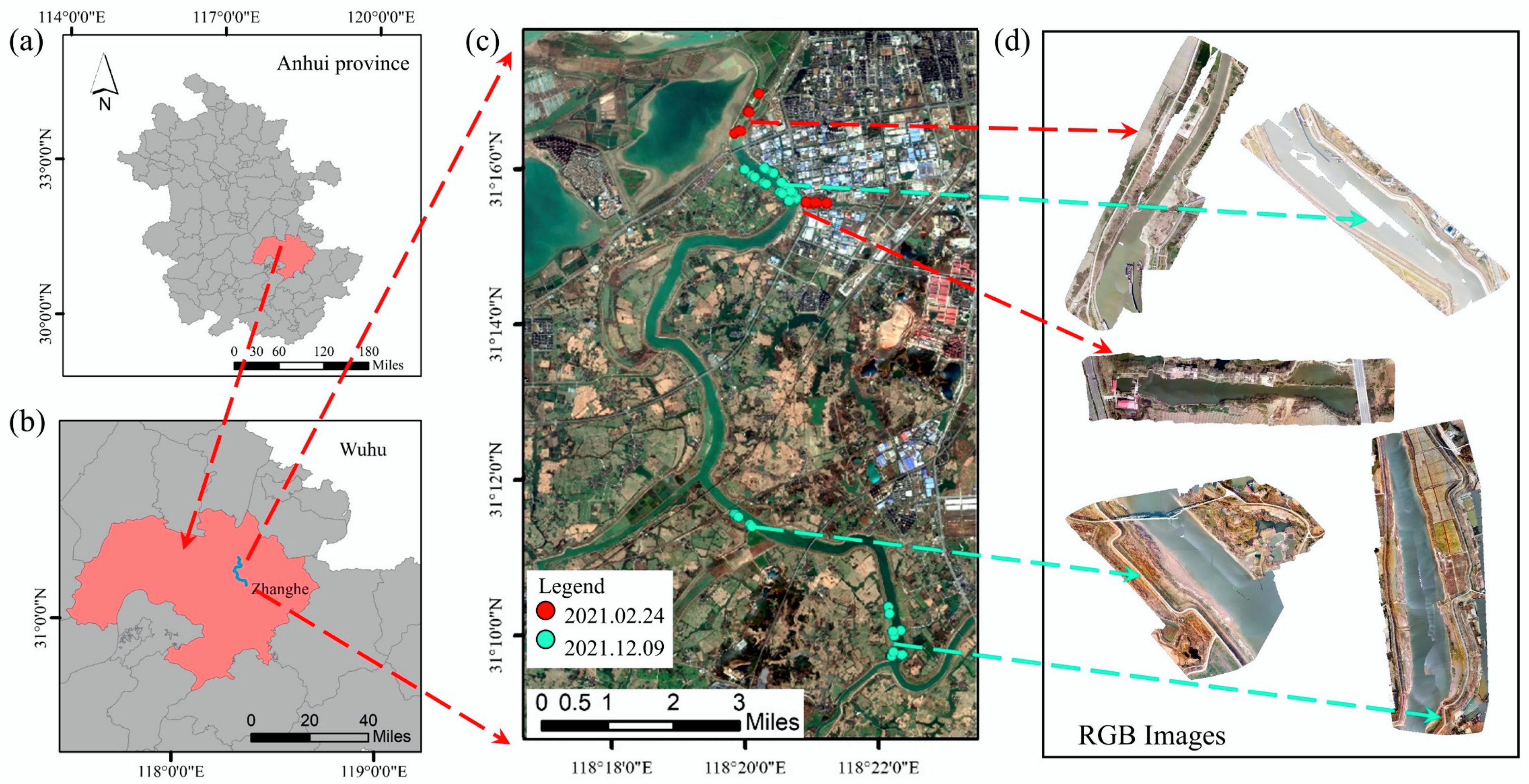
The Zhanghe River, located in the city of Wuhu in Anhui Province, China, flows into the Yangtze River from Nanling County. The Yangtze River, which is the largest river in China with important economic, ecological, and social benefits, is an essential source of drinking water for the country as well as a habitat for many species [42]. The dry season in this region persists from November through to March of the following year, and the low flow during the dry season has substantial impact on the aquatic ecosystem, including water quality, which causes serious environmental problems [43]. Monitoring the water quality of the tributaries of the Yangtze River throughout the dry season is absolutely critical. Therefore, this study conducted sampling in the downstream region of the Zhanghe River during the dry season. Figure 1 displays the geographic location of the study area and the distribution of the sampling points.
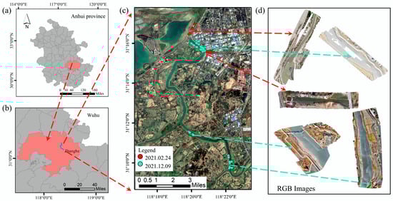
Figure 1.
Geographic location of the study area and the distribution of the selected sampling points: (a) location of Anhui Province, (b) location of the city of Wuhu, (c) location of water sampling points on the Zhanghe River, and (d) examples of UAV-derived RGB orthophotography of the research river sections.
2.2. Data Collection and Processing
2.2.1. UAV Multispectral Image Collection and Preprocessing
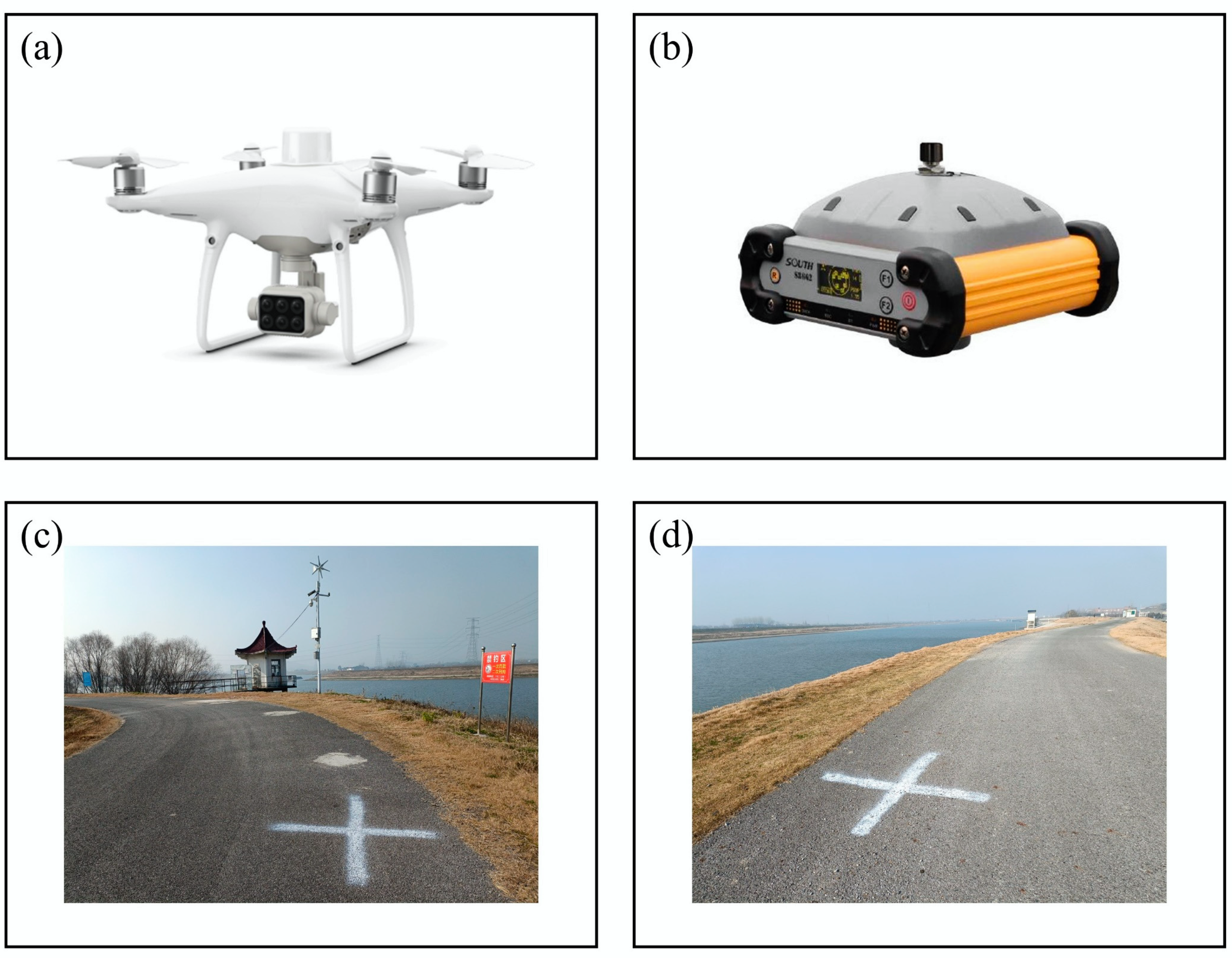
In this study, the DJI P4 Multispectral UAV (DJI, Shenzhen, Guangdong, China) was employed as the platform for acquiring high-resolution multispectral photographs (Figure 2a). The platform was equipped with a multispectral camera with six 1/2.9-inch CMOS (Complementary Metal Oxide Semiconductor) sensors, comprising a color sensor for RGB imaging and five monochromatic sensors for multispectral imaging. Thus, it could collect images in the blue, green, red, red-edge, and near-infrared bands, simultaneously. Image resolution was 1600 × 1300 pixels with a 5.74 mm focal lens (https://www.dji.com/cn/p4-multispectral/specs (accessed on 18 May 2022)). Table 1 lists the central wavelength and half-maximum wave width of each band.
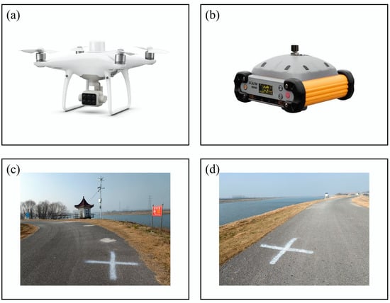
Figure 2.
Instruments and ground control points (GCPs): (a) DJI P4 Multispectral UAV, (b) RTK S86 system, and (c,d) examples of the GCPs.

Table 1.
Spectral region and wavelength range of the UAV-derived multispectral images.
In February and December 2021, high-resolution multispectral images of five downstream sections of the Zhanghe River were collected. The UAV operational altitude was 120–150 m, the course overlap degree was set at 80%, and the side overlap degree was set at 70%. Mirror reflection, aquatic vegetation, and atmospheric effects can all have strong impacts on the inversion of the spatiotemporal changes in water quality based on remote sensing data. Water highlights and flares induced by mirror reflection are the most influential factors in UAV water quality inversion [44,45]. To reduce specular reflection, all UAV images were taken between 13:00 and 16:00 local time. Mosaic images were generated using pix4D, and then resampled in ENVI to achieve 0.10 m spatial resolution. Before the flight mission, 21 ground control points (GCPs) were established on both sides of the river to improve the spatial precision of the mosaic images, and the precise coordinates were measured using the Real-Time Kinematic (RTK) S86T system (Figure 2b). The gaussian projection was utilized in GCPs coordinate measurement, and the projection coordinate system was CGCS2000. The antenna was raised to a height of 2 m using a support pole, and data were recorded when the fixed solution was presented. Examples of the GCPs are shown in Figure 2c,d. Table 2 lists the precise coordinates of each GCP.
Table 2.
Coordinates of the ground control points (GCPs) measured using the RTK S86T system.
The operational altitude of the UAV was sufficiently low that atmospheric refraction could be ignored [25]. The values of each band were standardized according to Equation (1) to facilitate the following quantitative analysis [46]. A single pixel can easily be impacted by specular reflection and water splash, making it difficult to reflect the spectral difference induced by an actual change in water quality at the sampling point. The accuracy of the inversion model can be improved by selecting an appropriate window size and noise removal approach.
where DN represents the digital number of each band, and DNmin and DNmax represent the minimum and maximum DN of a single band in the image, respectively. The calculated spectral response value ranged from 0 to 1.
2.2.2. Ground Monitoring Data
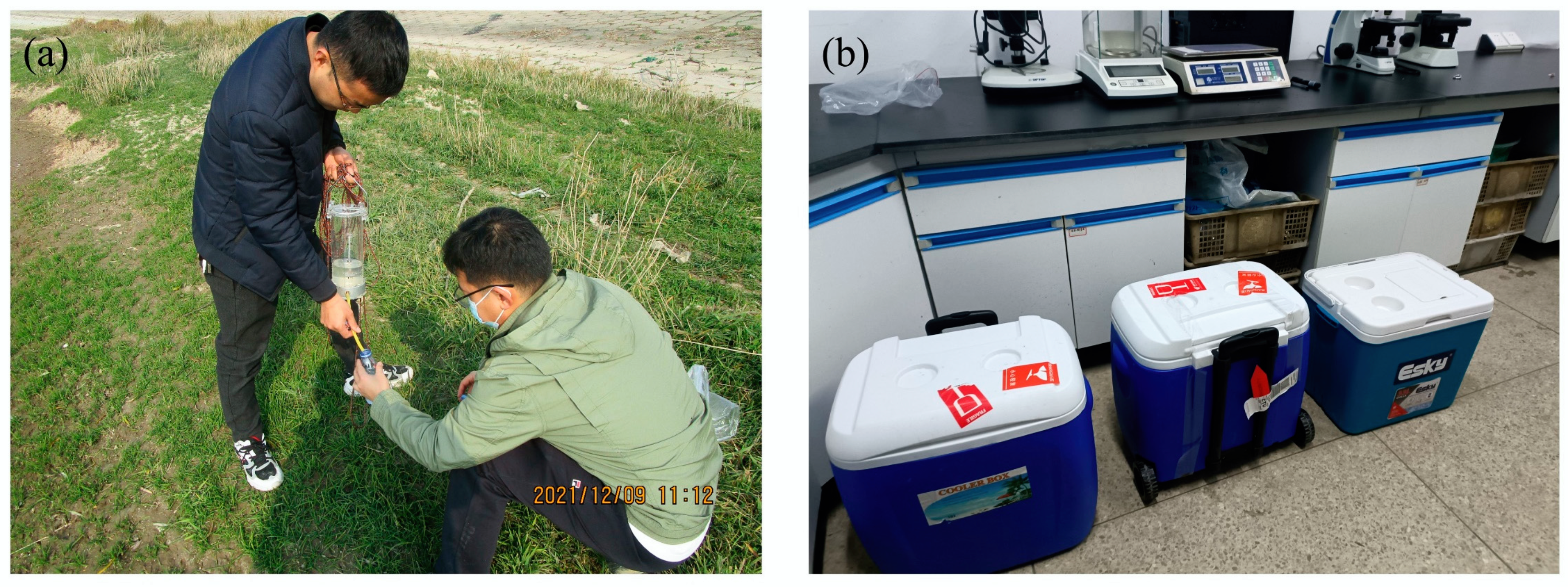
In total, 45 valid water samples were collected from the Zhanghe River (13 samples in February and 32 samples in December 2021). At each sampling point, 1 L of water was taken at a depth of 50 cm below the water surface using a sampler and transported to a storage container. All samples were held in an ice-filled thermostat until delivered to the laboratory for testing and analysis (Figure 3). The water quality parameters included Chl-a, TN, TP, and CODMn. The testing process was based on the Chinese national standard and trade standard, and the standards adopted for Chl-a, TN, TP and CODMn were HJ 828-2017, HJ 636-2012, GB 1189-1989, and GB 11892-1989, respectively. A workflow chart of the data processing procedure is shown in Figure 4.

Figure 3.
Photographs of field water sample collection and storage: (a) collection of a water sample from the Zhanghe River and (b) water sample storage.

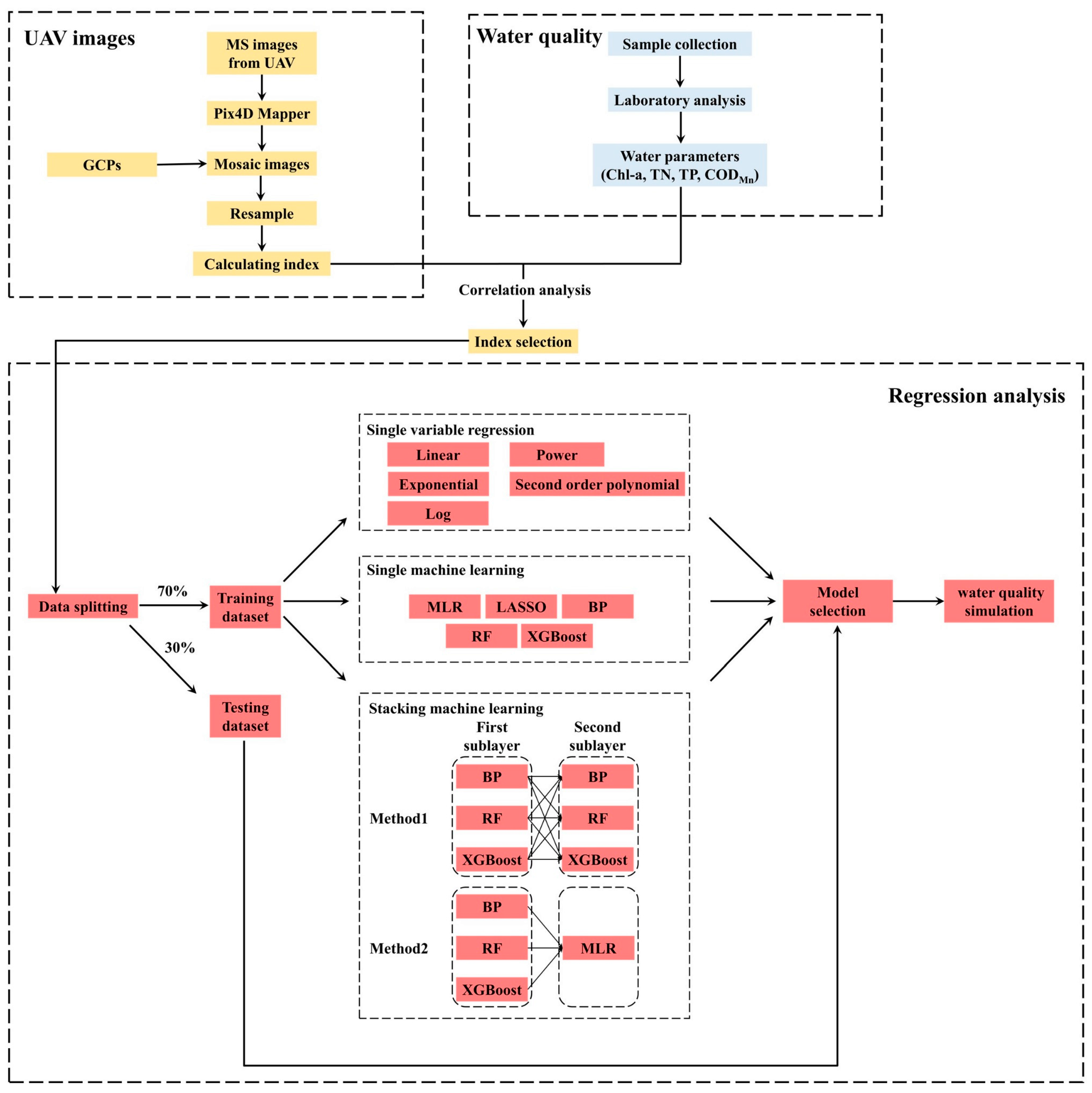
Figure 4.
Workflow chart of the data processing procedure.
2.3. Method
2.3.1. Calculation of Spectral Index
A typical spectral index used in water quality remote sensing inversion is the double-band combination, which can remove noise interference, emphasize the spectral features of water quality parameters, and substantially increase the accuracy of the water quality inversion model [47,48]. In this study, any two of the five single bands were handled using band sum, band difference, and band ratio, resulting in 45 double band combinations (Table 3). Pearson correlation analysis was performed on the measured data of each water quality parameter and each band combination to determine the best band combination for constructing a water quality inversion model.
Table 3.
Band combination construction and calculation. Note: labels V1–V45 represent the number of each index.
2.3.2. Traditional Regression Methods
After selecting the spectral indices, various classical regression models and ML models were built to determine the best modeling strategy for each parameter. The following techniques were considered: linear regression, exponential regression, logarithmic regression, second-order polynomial regression, power regression, Multiple Linear Regression (MLR), Least Absolute Shrinkage and Selection Operator (LASSO), BP, RF, and XGBoost.
MLR is a commonly used linear regression model that can statistically explain the linear relationship between the dependent variable and several independent variables and provide better predictions than single-variable regression models [49,50]. MLR presents the advantage of simplicity and computational efficiency, but it is incapable of fitting non-linear data since it is based on the assumption that the independent and dependent variables have a linear relationship.
Lasso is a biased estimating method proposed by Tibshirani in 1996 that is commonly utilized in regression models for variable selection and parameter estimation. By adding restrictions to the coefficients, LASSO eliminates the impact of multicollinearity in the model [51]. It has produced promising results in variable selection and prediction.
BP is a multilayer feed-forward network based on the error back propagation method, which is particularly good at handling non-linear and uncertain problems. The BP consists of input layers, implicit layers and output layers, and contains two stages: forward propagation and back propagation of the error [52]. The error is back-propagated through the implicit layer to the output layer, and apportioned to all units in each layer, until the error is eventually decreased to an acceptable level after continual training [53].
RF is an ML algorithm based on decision trees that was developed by Breiman in 2001 [54]. RF extracts several Bootstrap samples from the original sample for decision tree modeling, then merges multiple decision trees for prediction, and finally derives the prediction result by voting. Because of its high classification and prediction accuracy, RF is widely used in remote sensing image classification and big data analysis [55,56].
The XGBoost algorithm, which Chen developed in 2016, is based on regression trees. It improves the operational efficiency of the optimization process while reducing overfitting by employing second-order derivative data and integrating a regular component in the cost function [57,58].
The band combination with the highest correlation was treated as an input variable in a single-variable regression analysis, and the water quality parameters were modeled as output variables. The three band combinations having the greatest correlation with each water quality metric were utilized as input variables in multivariate regression analyses, and each water quality parameter was used as an output variable for modeling. During the model construction process, 70% of the data with a certain concentration gradient were chosen for the training dataset and 30% were chosen for the testing dataset.
2.3.3. Stacking ML Method
The stacking ML method takes a typical ensemble model based on different learners in which the training data are fed into the first-layer ML model, and the output of the first layer is used as the input of the second layer. This process represents a further search for better approximation based on the first-layer output, which is important for mitigating the risk of overfitting and thus obtaining better prediction results than are realized when using a single ML model [59,60].
2.3.4. Accuracy Evaluation
Pearson correlation analysis was performed on the spectral indices and the water quality parameters, and Pearson’s r was used to assess the relationship between the spectral index and the water quality parameters. The greater the value of Pearson’s r, the stronger the relationship between the spectral index and the water quality measures. Additionally, the coefficient of determination (R2), root mean square error (RMSE), and mean absolute error (MAE) were used to quantify the accuracy and performance of the model using new data (Equations (2)–(4), respectively). Statistical analysis of the parameters, calculation of the correlation coefficients, and the error analysis were mainly realized using R 4.1.2.
where R2 is the coefficient of determination, RMSE is the root mean square error, MAE is the mean absolute error, represents the predicted values of the water quality parameters, yi represents the measured values of the water quality parameters, and n is the number of sampling points.
3. Results
3.1. Data Analysis
Table 4 summarizes the statistical analysis of the concentrations of the water quality parameters sampled in the two periods (i.e., mean value (Mean), maximum value (Max), minimum value (Min), and standard deviation (SD)).
Table 4.
Analysis of measured water quality data of the two sampling periods. SD represents the standard deviation, and N represents the number of sampling points. Units are μg L−1 for Chl-a, and mg L−1 for TN, TP, and CODMn.
The concentration of Chl-a at each sampling point ranged from 6.00–74.00 μg L−1 on 20 February 2021, and the mean (±SD) was 33.62 ± 25.60 μg L−1. The concentration of Chl-a at each sampling point ranged from 1.00–13.50 μg L−1 from 9–10 December 2021, and the mean (±SD) was 4.81 ± 2.76 μg L−1. The Chl-a concentration was low in December, whereas the concentration in February 2021 was higher, indicating the possibility of the occurrence of the bloom phenomenon. Inversion of Chl-a at different concentration levels requires different spectral indices and algorithms [61], and the Chl-a concentration range of 0–15 μg L−1 was selected for the modeling and analysis in this study.
The GB 3838-2002 standard divides the environmental quality of surface water into Class I to Class V, for which the concentrations of TN, TP, and CODMn form the basis of the classification. The TN concentration at each sampling point ranged from 1.90–10.80 mg L−1 on 20 February 2021, and the mean (±SD) was 6.45 ± 3.29 mg L−1, i.e., the water quality at most sampling points exceeded the Class V standard. The TN concentration at each sampling point ranged from 1.12–4.58 mg L−1 from 9–10 December 2021, and the mean (±SD) was 2.88 ± 1.45 mg L−1. Therefore, some of the sampling points were classified as Class IV or V, while others exceeded the Class V water standard.
The TP concentration at each sampling point ranged from 0.09–0.38 mg L−1 on 20 February 2021, and the mean (±SD) was 0.23 ± 0.10 mg L−1, i.e., the water quality at most sampling points was between Class III and Class V. The TP concentrations at each sampling point ranged from 0.06–0.17 mg L−1 from 9–10 December 2021, and the mean (±SD) was 0.11 ± 0.03 mg L−1. Most of the sampling points were classified as Class II or Class III. The CODMn concentration at each sampling point ranged from 3.10–6.10 mg L−1 on 20 February 2021, and the mean (±SD) was 4.36 ± 1.01 mg L−1, i.e., most of the sampling points were classified as Class II or Class III. The CODMn concentration at each sampling point ranged from 2.80–4.90 mg L−1 from 9–10 December 2021, and the mean (±SD) was 3.96 ± 0.52 mg L−1. Most of the sampling points were classified as Class II or Class III. Overall, water quality in December 2021 was markedly better than that in February 2021. In the study area, the main pollutants were found to be TN and TP, which have relatively high concentrations in the water body.
3.2. Spectral Index Correlation Analysis
Figure 5 shows the magnitude of the correlation between the 45 constructed spectral indices and each water quality parameter. The Chl-a concentration was correlated positively with most of the spectral indices, the TN and TP concentrations were more significantly negatively correlated with most of the spectral indices, while CODMn and most of the spectral values showed weak negative correlation. The three spectral indices that had the strongest correlation with the water quality parameters were defined as the sensitive indices of the water quality parameters, and were used for subsequent model building and the following analysis. Ultimately, B1 + B2, (B1 − B5)/(B1 + B5), and (B3 − B5)/(B3 + B5) were the sensitive indices for Chl-a, B1, B1 + B4, and B1 + B5 were the sensitive indices for TN, (B1 − B4)/(B1 + B4), (B1 − B5)/(B1 + B5), and (B3 − B5)/(B3 + B5) were the sensitive indices for TP, and (B1 − B5)/(B1 + B5), (B2 − B5)/(B2 + B5), and (B3 − B4)/(B3 + B4) were the sensitive indices for CODMn.
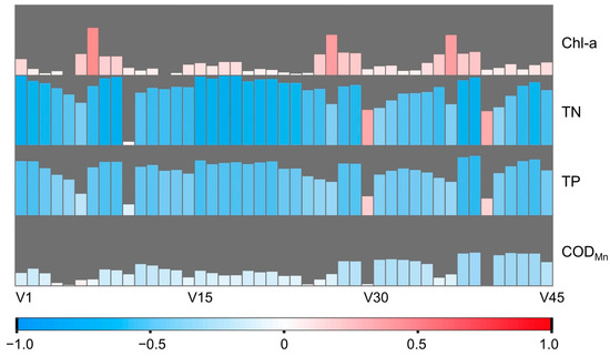
Figure 5.
The correlation between spectral index and water quality parameters.
3.3. Results of Simple Regression Methods
As input variables for the single-variable regression models, the spectral values with the strongest correlation with each water quality parameter were used. The precision effects of the single-variable regression models are presented in Table 5. For the training dataset, the R2 values were in the range of 0.247–0.263, 0.579–0.693, 0.455–0.630, and 0.120–0.209 for Chl-a, TN, TP, and CODMn, respectively, with corresponding RMSEs in the range of 2.055–2.135 μg L−1, 1.556–3.001 mg L−1, 0.049–0.055 mg L−1, and 0.549–0.579 mg L−1, respectively. For the testing dataset, the R2 values were in the range of 0.170–0.203, 0.597–0.662, 0.376–0.431, and 0.107–0.204 for Chl-a, TN, TP, and CODMn, respectively.
Table 5.
Single-variable regression results of water quality parameters. Note: “-” represents the presence of negative values of the spectral index, and thus the logarithmic and power functions could not be fitted.
Table 6 presents the optimal single-variable regression model for each parameter and its accuracy. Linear regression, exponential regression, power regression, and second-order polynomial regression were found to be the best approaches for Chl-a, TN, TP, and CODMn, respectively. Although the optimal single regression approach for each water quality parameter varied, it was straightforward to conclude that the accuracy of the nonlinear model with all other factors except Chl-a was much better than that of the linear model.
Table 6.
Simple optimal single-variable regression model for each water quality parameter.
3.4. Comparison of Results of ML Models and Stacked ML Models
Figure 6 presents the model testing accuracy of five single ML models for various water quality parameters for MLR, Lasso, BP, RF, and XGBoost. The input variables for each ML model were the three spectral indices that exhibited the strongest correlation with the corresponding water quality parameters. Overall, the TN inversion model produced the best prediction (R2 values in the range of 0.642–0.822, RMSE in the range of 1.273–1.499 mg L−1, and MAE in the range of 0.843–1.279 mg L−1), and the CODMn inversion model produced the poorest prediction (R2 values in the range of 0.060–0.224, RMSE in the range of 0.796–0.860 mg L−1, and MAE in the range of 0.685–0.794 mg L−1). With a comparatively high R2 value and low RMSE and MAE, BP was the best single ML modeling approach for TN (R2 = 0.822, RMSE = 1.273 mg L−1, and MAE = 0.843 mg L−1), TP (R2 = 0.822, RMSE = 1.273 mg L−1, and MAE = 0.843 mg L−1), and CODMn (R2 = 0.224, RMSE = 0.796 mg L−1, and MAE = 0.685 mg L−1). XGBoost was the best single ML modeling approach for Chl-a (R2 = 0.415, RMSE = 2.074 μg L−1, and MAE = 1.521 μg L−1).
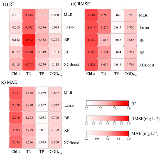
Figure 6.
Comparison of predicted and measured water quality parameters using different single ML methods: (a) R2, (b) RMSE, and (c) MAE.
The modeling impacts of several single ML and stacked ML models for Chl-a are shown in Table 7. The stacking ML method substantially enhances the fitting effects of the training dataset, with R2 values increased from 0.247–0.958 to 0.690–0.999, RMSE decreased from 0.801–2.021 to 0.019–1.338 μg L−1, and MAE decreased from 0.478–1.520 to 0.017–1.051 μg L−1. Stacked ML models based on different combinations of single ML models produced varied prediction results for the testing dataset. Among these, the Chl-a inversion model constructed using the RF-XGBoost method outperformed the best single ML model (XGBoost), i.e., for the testing dataset, R2 increased from 0.415 to 0.504, RMSE decreased from 2.074 to 1.770 μg L−1, and MAE decreased from 1.521 to 1.272 μg L−1.
Table 7.
Comparison of the performance of single ML models and stacked ML models for Chl-a.
Table 8 presents the modeling effects of different single ML and stacked ML models for TN. The R2, RMSE, and MAE values for the single ML models with the training dataset were in the range of 0.589–0.956, 0.579–1.764 mg L−1, and 0.434–1.417 mg L−1, respectively, whereas the R2, RMSE, and MAE values for the stacked ML models were in the range of 0.910–0.977, 0.423–0.959 mg L−1, and 0.279–0.750 mg L−1, respectively. The R2, RMSE, and MAE values of the single ML models for the testing dataset were in the range of 0.642–0.822, 1.273–1.499 mg L−1, and 0.843–1.279 mg L−1, respectively, and the R2, RMSE, and MAE values of the stacked ML models were in the range of 0.700–0.839, 1.089–1.494 mg L−1, and 0.632–1.042 mg L−1, respectively. The results indicate that the improvement of the stacked ML models was substantial. The TN inversion model constructed using the BP-RF methods outperformed the best single ML model (XGBoost).
Table 8.
Comparison of the performance of single ML models and stacked ML models for TN.
Table 9 presents the modeling effects of different single and stacked ML models for TP. For the training dataset, the R2, RMSE, and MAE values of the single ML models were in the range of 0.545–0.958, 0.019–0.055 mg L−1, and 0.015–0.040 mg L−1, respectively, whereas the R2, RMSE, and MAE values of the stacked ML models were in the range of 0.835–0.963, 0.016–0.035 mg L−1, and 0.012–0.035 mg L−1, respectively. For the testing dataset, the R2, RMSE, and MAE values for the single ML models were in the range of 0.279–0.432, 0.053–0.073 mg L−1, and 0.044–0.047 mg L−1, respectively, while the R2, RMSE, and MAE values for the stacked ML models were in the range of 0.241–0.347, 0.062–0.077 mg L−1, and 0.042–0.050 mg L−1, respectively. Although the stacked ML models outperformed individual ML models with the training dataset, they produced poorer accuracy with the testing dataset.
Table 9.
Comparison of the performance of single ML models and stacked ML models for TP.
Table 10 presents the modeling effects of different single ML and stacked ML models for CODMn. For the training dataset, the R2, RMSE, and MAE values for the single ML models were in the range of 0.144–0.911, 0.257–0.573 mg L−1, and 0.221–0.487 mg L−1, respectively, and the R2, RMSE, and MAE values for the stacked ML models were in the range of 0.884–0.980, 0.115–0.273 mg L−1, and 0.091–0.206 mg L−1, respectively. For the testing dataset, the R2, RMSE, and MAE values for the single ML models were in the range of 0.060–0.224, 0.796–0.860 mg L−1, and 0.685–0.794 mg L−1, respectively, and the R2, RMSE, and MAE values for the stacked ML models were in the range of 0.130–0.272, 0.767–0.851 mg L−1, and 0.674–0.771 mg L−1, respectively. For both the training dataset and the testing dataset, the stacked ML models were successful in CODMn modeling, i.e., the BP-RF method outperformed the BP method., which is the optimal single ML model.
Table 10.
Comparison of the performance of single ML models and stacked ML models for CODMn.
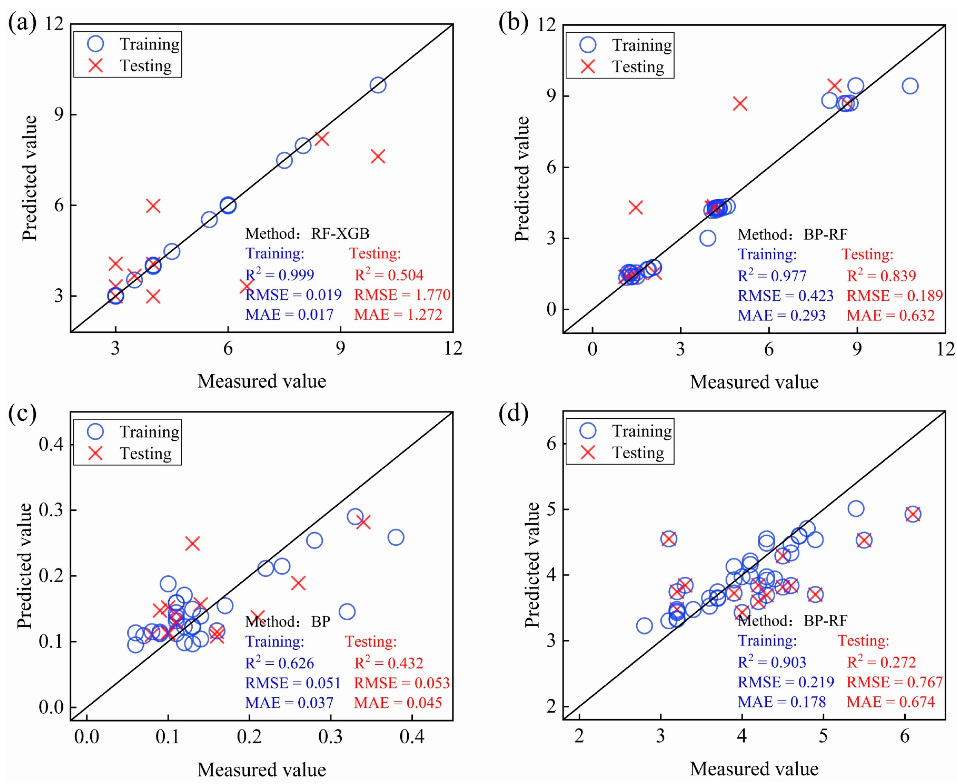
The measured values and the values predicted using the optimal modeling approach for each water quality parameter are shown in Figure 7 for comparison purposes.
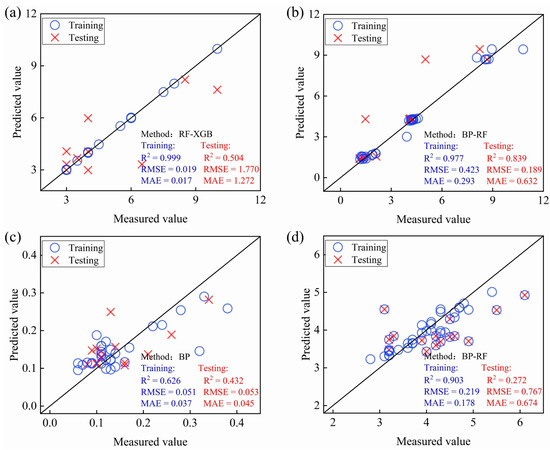
Figure 7.
Scatter plots of measured water quality values and optimal model predicted values: (a) Chl-a, (b) TN, (c) TP, and (d) CODMn.
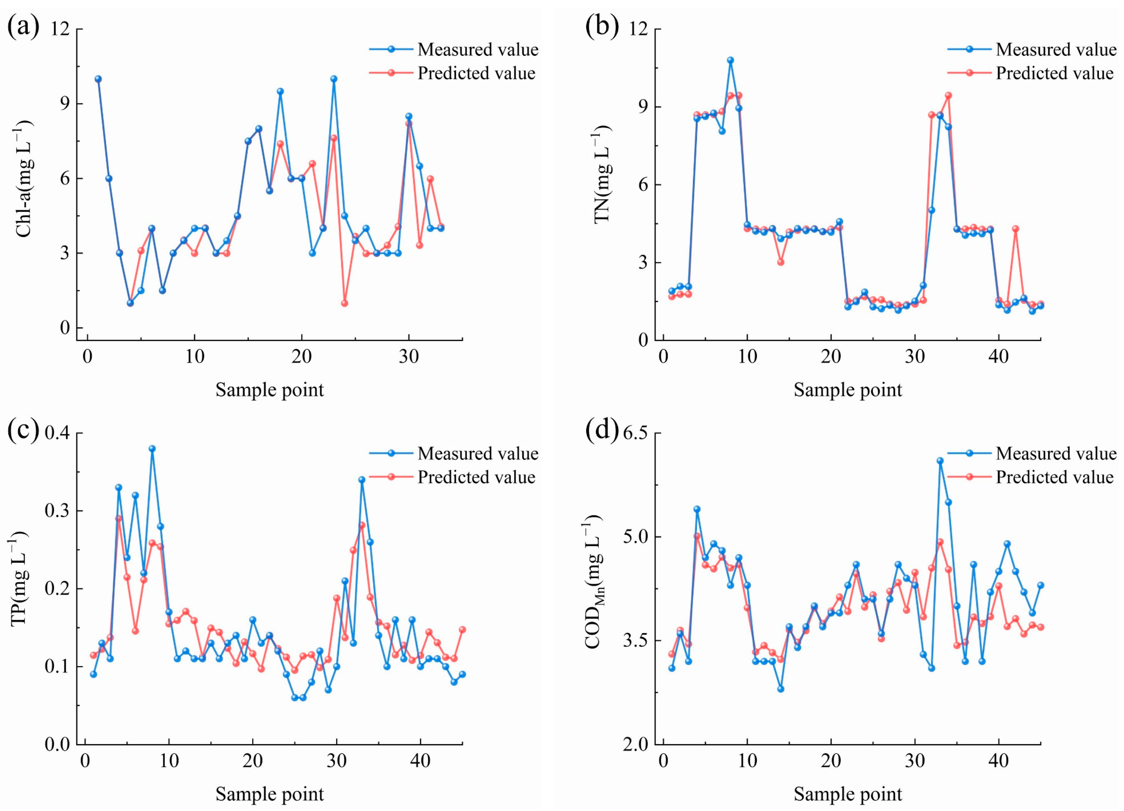
Figure 8 shows a comparison of the observed values of water quality at each sample point and the values predicted using the approach selected from Figure 7. It can be seen that the inversion model better reflects the water quality of the water bodies.
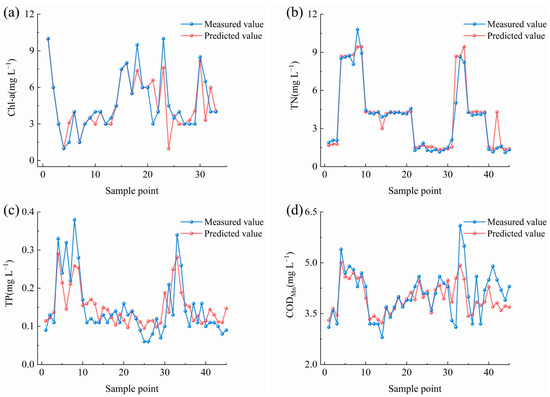
Figure 8.
Comparison of measured and predicted values: (a) Chl-a, (b) TN, (c) TP, and (d) CODMn.
4. Discussion
4.1. Performance of Stacked ML Models in Monitoring Water Quality
The main purpose of this research was to develop a stacked ML model that could be used to invert water quality parameters using UAV multispectral images and small amounts of ground-based water quality data. Five single-variable regression models (linear regression, exponential regression, power regression, logarithmic function regression, and second-order polynomial regression) and five typical ML models (MLR, Lasso, RF, BP, and XGBoost) were compared to evaluate the robustness and applicability of stacked ML models. The results show that both the single-variable regression models and the multivariate regression models (i.e., the nonlinear methods) outperformed the linear methods (except the single-variable regression model for Chl-a), which is consistent with previous findings [62,63]. Additionally, the stacked ML models outperformed traditional single-variable regression models and single ML models, indicating that stacked ML models offer unparalleled advantages in terms of water quality inversion and thus have great potential for water quality monitoring research. Furthermore, the results revealed that the prediction effect of stacked ML models generated using different ML combinations varied greatly, with the fitting effect of the training dataset far outweighing that of the testing dataset. In particular, for TP, the stacked ML models substantially enhance the fitting effect of the training dataset when compared with individual ML models; however, the fitting effect for the testing dataset was lowered, implying that the models remain at risk of overfitting.
This overfitting phenomenon exists not only in stacked ML models but also in single ML models. Previously, the first stage of stacked ML models usually incorporated several groups of ML methods, and the input for the second stage was the output result of multiple groups of single ML models. To avoid overfitting, the second-stage ML method was usually a simple learner (e.g., MLR), but this method still has limitations in our opinion. In this study, the inputs and outputs of the first stage of the stacked ML methods were fed into the second stage simultaneously (i.e., the inputs of the second stage contained both the spectral indices and the prediction results from the first-stage ML methods). Table 6, Table 7, Table 8 and Table 9 present results that demonstrate that the proposed modification was effective, and that the model built using the more general ML-MLR method was not the best stacked ML model for each parameter. Moreover, the small sample size of the data used for training might explain why overfitting occurs, i.e., the model learned too much about the individual characteristics of the data without learning the substantive discipline of the data [64,65]. Therefore, obtaining more sample data in future research is critically important for building a water quality inversion model with high applicability and accuracy.
4.2. Differences in Inversion Models for Different Water Quality Parameters
The water quality parameters investigated in this study were Chl-a, TN, TP, and CODMn. Previous studies have shown that Chl-a is an optically sensitive parameter with significant optical activity characteristics [66], whereas TN, TP, and CODMn are non-optical sensitive parameters [67], and that it is usually difficult to obtain accurate quantitative predictions of their concentrations and spatial distributions based on satellite remote sensing images and simple statistical analysis models [68]. High-resolution images captured by a UAV and the emergence of advanced artificial intelligence algorithms have brought new opportunities for quantitative remote sensing inversion of water quality parameters that are not optically sensitive [24]. Many studies have elucidated the great advantages of artificial intelligence algorithms in the inversion of water quality parameters that are not optically sensitive [69,70,71], and our research confirms the notable advantages of using ML (including stacked ML) algorithms for inversion of water quality using UAV multispectral images. As shown in Table 5, the optimal model for single-variable regression analysis was the linear regression method for Chl-a only, while the optimal model for each of the other parameters was a nonlinear model. This pattern also exists in the multivariate regression analysis, as shown in Figure 5. For the single ML algorithm, the optimal algorithm for Chl-a was XGBoost, while the optimal algorithm for each of the other parameters was BP. Therefore, we argue that there are considerable differences in the algorithms most applicable to the inversion of parameters that are optically sensitive and to that of parameters that are not. The differences between the two types of parameters should be fully considered in future modeling, and different algorithms should be used for inversion model construction.
4.3. Limitations and Perspectives
UAVs can provide high-frequency observational data with large spatial coverage, which have an important role in the high-frequency observation of the regional spatiotemporal dynamics of water bodies. However, few relevant studies have been conducted and the related theories and methods remain immature. Inland water bodies have complex optical properties that are affected by suspended matter, colored dissolved organic matter, and bottom reflection of shallow water [72]. Remote sensing reflectance is a typical apparent optical property that can be used to accurately define the optical characteristics of a water body and is employed extensively in water quality inversion. However, accurate radiometric calibration for UAV-derived multispectral images is a difficult task owing to the different imaging times and surroundings of each photo [73]. Meanwhile, radiation transmission in a water body depends on the inherent optical properties that are independent of the distribution and intensity of the light field around the medium. Thus, the inversion of water quality parameters has a direct or indirect relationship with the inherent optical properties, and the absorption coefficient and other inherent optical properties directly determine the remote sensing reflectance and other common apparent optical properties. Consideration of the inherent optical characteristics of the different components of a water body is an important element in achieving optical monitoring of water quality [74,75]. Furthermore, previous research has shown that a wide bandwidth makes it difficult to separate the optical characteristics of various components of a water body with complex optical properties [76]; however, the development and application of hyperspectral sensors is an important approach to resolving this problem. Recent research has demonstrated that the use of artificial intelligence (especially deep learning methods) in water quality inversion (including parameters that are not optically sensitive) has considerable potential for reducing error [77]. In the future, hyperspectral sensors with additional bands, narrower bandwidths, and more advanced artificial intelligence methods will be used to analyze both the inherent and the apparent optical quantities of water bodies to better explain the optical properties of inland water bodies and achieve accurate monitoring of water quality.
5. Conclusions
In this study, various spectral indices with double-band combinations were constructed, and the optimal indices for modeling were selected on the basis of linear correlation analysis between the band combination and water quality concentration. Univariate regression methods, ML regression methods, and stacked ML methods were used to construct separate water quality inversion models for Chl-a, TN, TP, and CODMn. The results show that stacked ML models had higher R2 values and smaller RMSEs and MAEs. Stacked ML algorithms demonstrated notable advantages in terms of water quality inversion, and predicted water quality changes and spatial distributions more effectively and more accurately than other methods. Additionally, the best modeling approach was found to differ for different parameters, and the availability of optical activity might become one of the standards with which to distinguish the most appropriate modeling approach. Consequently, future research should strongly consider the adoption of stacked ML algorithms to monitor spatiotemporal changes in water quality.
Author Contributions
Conceptualization and methodology, Y.X., Y.G. and Y.F.; software, Y.X. and Y.G.; validation, Y.X., Y.G., G.Y., X.Z., Y.S., F.H. and Y.F.; formal analysis, Y.X., Y.G. and X.Z.; investigation, Y.X., Y.G., G.Y., X.Z. and Y.S.; resources, F.H. and Y.F.; data curation, Y.X., Y.G. and G.Y.; writing—original draft preparation, Y.X.; writing—review and editing, Y.X., Y.G., X.Z., Y.S., F.H. and Y.F.; visualization, Y.X.; supervision, Y.F.; project administration, F.H. and Y.F.; funding acquisition, F.H. and Y.F. All authors have read and agreed to the published version of the manuscript.
Funding
This study was funded by the joint fund for regional innovation and development of NSFC (Grant No. U21A2039), the National Funds for Distinguished Young Youths (Grant No. 42025101) and the 111 Project (Grant No. B18006).
Data Availability Statement
Not applicable.
Acknowledgments
We appreciate Shouzhi Chen for collecting UAV images, Xinxi Li and Qingping Liu for collecting water sample. Additionally, we also thank Xuhao Li for his help on UAV operation and data analysis.
Conflicts of Interest
The authors declare no conflict of interest.
References
- Fezzi, C.; Harwood, A.R.; Lovett, A.A.; Bateman, I.J. The environmental impact of climate change adaptation on land use and water quality. Nat. Clim. Chang. 2015, 5, 255–260. [Google Scholar] [CrossRef] [Green Version]
- Zhao, Z.; Cao, Y.; Fan, Y.; Yang, H.; Feng, X.; Li, L.; Zhang, H.; Xing, L.; Zhao, M. Ladderane records over the last century in the East China sea: Proxies for anammox and eutrophication changes. Water Res. 2019, 156, 297–304. [Google Scholar] [CrossRef] [PubMed]
- Basu, N.B.; Van Meter, K.J.; Byrnes, D.K.; Van Cappellen, P.; Brouwer, R.; Jacobsen, B.H.; Jarsjo, J.; Rudolph, D.L.; Cunha, M.C.; Nelson, N.; et al. Managing nitrogen legacies to accelerate water quality improvement. Nat. Geosci. 2022, 15, 97–105. [Google Scholar] [CrossRef]
- Zhang, M.; Wang, L.; Mu, C.; Huang, X. Water quality change and pollution source accounting of Licun River under long-term governance. Sci. Rep. 2022, 12, 2779. [Google Scholar] [CrossRef] [PubMed]
- Tao, T.; Xin, K. A sustainable plan for China’s drinking water. Nature 2014, 511, 527–528. [Google Scholar] [CrossRef] [PubMed]
- Determan, R.T.; White, J.D.; McKenna, L.W., III. Quantile regression illuminates the successes and shortcomings of long-term eutrophication remediation efforts in an urban river system. Water Res. 2021, 202, 117434. [Google Scholar] [CrossRef] [PubMed]
- Guan, Q.; Feng, L.; Hou, X.; Schurgers, G.; Zheng, Y.; Tang, J. Eutrophication changes in fifty large lakes on the Yangtze Plain of China derived from MERIS and OLCI observations. Remote Sens. Environ. 2020, 246, 111890. [Google Scholar] [CrossRef]
- Odermatt, D.; Gitelson, A.; Brando, V.E.; Schaepman, M. Review of constituent retrieval in optically deep and complex waters from satellite imagery. Remote Sens. Environ. 2012, 118, 116–126. [Google Scholar] [CrossRef] [Green Version]
- Feng, L.; Dai, Y.; Hou, X.; Xu, Y.; Liu, J.; Zheng, C. Concerns about phytoplankton bloom trends in global lakes. Nature 2021, 590, E35–E47. [Google Scholar] [CrossRef]
- Zhang, Y.; Zhou, L.; Zhou, Y.; Zhang, L.; Yao, X.; Shi, K.; Jeppesen, E.; Yu, Q.; Zhu, W. Chromophoric dissolved organic matter in inland waters: Present knowledge and future challenges. Sci. Total Environ. 2021, 759, 143550. [Google Scholar] [CrossRef]
- Doernhoefer, K.; Oppelt, N. Remote sensing for lake research and monitoring—Recent advances. Ecol. Indic. 2016, 64, 105–122. [Google Scholar] [CrossRef]
- Aurin, D.; Mannino, A.; Franz, B. Spatially resolving ocean color and sediment dispersion in river plumes, coastal systems, and continental shelf waters. Remote Sens. Environ. 2013, 137, 212–225. [Google Scholar] [CrossRef] [Green Version]
- Shi, J.; Shen, Q.; Yao, Y.; Li, J.; Chen, F.; Wang, R.; Xu, W.; Gao, Z.; Wang, L.; Zhou, Y. Estimation of Chlorophyll-a Concentrations in Small Water Bodies: Comparison of Fused Gaofen-6 and Sentinel-2 Sensors. Remote Sens. 2022, 14, 229. [Google Scholar] [CrossRef]
- Sagan, V.; Peterson, K.T.; Maimaitijiang, M.; Sidike, P.; Sloan, J.; Greeling, B.A.; Maalouf, S.; Adams, C. Monitoring inland water quality using remote sensing: Potential and limitations of spectral indices, bio-optical simulations, machine learning, and cloud computing. Earth-Sci. Rev. 2020, 205, 103187. [Google Scholar] [CrossRef]
- Templin, T.; Popielarczyk, D.; Kosecki, R. Application of Low-Cost Fixed-Wing UAV for Inland Lakes Shoreline Investigation. Pure Appl. Geophys. 2018, 175, 3263–3283. [Google Scholar] [CrossRef] [Green Version]
- Acharya, B.S.; Bhandari, M.; Bandini, F.; Pizarro, A.; Perks, M.; Joshi, D.R.; Wang, S.; Dogwiler, T.; Ray, R.L.; Kharel, G.; et al. Unmanned Aerial Vehicles in Hydrology and Water Management: Applications, Challenges, and Perspectives. Water Resour. Res. 2021, 57, e2021WR029925. [Google Scholar] [CrossRef]
- Guo, Y.; Chen, S.; Fu, Y.H.; Xiao, Y.; Wu, W.; Wang, H.; de Beurs, K. Comparison of Multi-Methods for Identifying Maize Phenology Using PhenoCams. Remote Sens. 2022, 14, 244. [Google Scholar] [CrossRef]
- Sun, X.; Zhang, Y.; Shi, K.; Zhang, Y.; Li, N.; Wang, W.; Huang, X.; Qin, B. Monitoring water quality using proximal remote sensing technology. Sci. Total Environ. 2022, 803, 149805. [Google Scholar] [CrossRef]
- Xiang, T.-Z.; Xia, G.-S.; Zhang, L. Mini-Unmanned Aerial Vehicle-Based Remote Sensing Techniques, applications, and prospects. IEEE Geosci. Remote Sens. Mag. 2019, 7, 29–63. [Google Scholar] [CrossRef] [Green Version]
- Yao, H.; Qin, R.; Chen, X. Unmanned Aerial Vehicle for Remote Sensing Applications-A Review. Remote Sens. 2019, 11, 1443. [Google Scholar] [CrossRef] [Green Version]
- Guo, Y.; Fu, Y.H.; Chen, S.; Bryant, C.R.; Li, X.; Senthilnath, J.; Sun, H.; Wang, S.; Wu, Z.; de Beurs, K. Integrating spectral and textural information for identifying the tasseling date of summer maize using UAV based RGB images. Int. J. Appl. Earth Obs. Geoinf. 2021, 102, 102435. [Google Scholar] [CrossRef]
- Chen, B.; Mu, X.; Chen, P.; Wang, B.; Choi, J.; Park, H.; Xu, S.; Wu, Y.; Yang, H. Machine learning-based inversion of water quality parameters in typical reach of the urban river by UAV multispectral data. Ecol. Indic. 2021, 133, 108434. [Google Scholar] [CrossRef]
- Zhang, Y.; Wu, L.; Ren, H.; Liu, Y.; Zheng, Y.; Liu, Y.; Dong, J. Mapping Water Quality Parameters in Urban Rivers from Hyperspectral Images Using a New Self-Adapting Selection of Multiple Artificial Neural Networks. Remote Sens. 2020, 12, 336. [Google Scholar] [CrossRef] [Green Version]
- Niu, C.; Tan, K.; Jia, X.; Wang, X. Deep learning based regression for optically inactive inland water quality parameter estimation using airborne hyperspectral imagery*. Environ. Pollut. 2021, 286, 117534. [Google Scholar] [CrossRef]
- Su, T.-C. A study of a matching pixel by pixel (MPP) algorithm to establish an empirical model of water quality mapping, as based on unmanned aerial vehicle (UAV) images. Int. J. Appl. Earth Obs. Geoinf. 2017, 58, 213–224. [Google Scholar] [CrossRef]
- Zhang, Y.; Wu, L.; Ren, H.; Deng, L.; Zhang, P. Retrieval of Water Quality Parameters from Hyperspectral Images Using Hybrid Bayesian Probabilistic Neural Network. Remote Sens. 2020, 12, 1567. [Google Scholar] [CrossRef]
- Sibanda, M.; Mutanga, O.; Chimonyo, V.G.P.; Clulow, A.D.; Shoko, C.; Mazvimavi, D.; Dube, T.; Mabhaudhi, T. Application of Drone Technologies in Surface Water Resources Monitoring and Assessment: A Systematic Review of Progress, Challenges, and Opportunities in the Global South. Drones 2021, 5, 84. [Google Scholar] [CrossRef]
- Mountrakis, G.; Im, J.; Ogole, C. Support vector machines in remote sensing: A review. ISPRS J. Photogramm. Remote Sens. 2011, 66, 247–259. [Google Scholar] [CrossRef]
- Pahlevan, N.; Smith, B.; Schalles, J.; Binding, C.; Cao, Z.; Ma, R.; Alikas, K.; Kangro, K.; Gurlin, D.; Nguyen, H.; et al. Seamless retrievals of chlorophyll-a from Sentinel-2 (MSI) and Sentinel-3 (OLCI) in inland and coastal waters: A machine-learning approach. Remote Sens. Environ. 2020, 240, 111604. [Google Scholar] [CrossRef]
- Guo, Y.; Fu, Y.; Hao, F.; Zhang, X.; Wu, W.; Jin, X.; Bryant, C.R.; Senthilnath, J. Integrated phenology and climate in rice yields prediction using machine learning methods. Ecol. Indic. 2021, 120, 106935. [Google Scholar] [CrossRef]
- Arias-Rodriguez, L.F.; Duan, Z.; de Jesus Diaz-Torres, J.; Hazas, M.B.; Huang, J.; Kumar, B.U.; Tuo, Y.; Disse, M. Integration of Remote Sensing and Mexican Water Quality Monitoring System Using an Extreme Learning Machine. Sensors 2021, 21, 4118. [Google Scholar] [CrossRef]
- Ma, Y.; Song, K.; Wen, Z.; Liu, G.; Shang, Y.; Lyu, L.; Du, J.; Yang, Q.; Li, S.; Tao, H.; et al. Remote Sensing of Turbidity for Lakes in Northeast China Using Sentinel-2 Images with Machine Learning Algorithms. IEEE J. Sel. Top. Appl. Earth Obs. Remote Sens. 2021, 14, 9132–9146. [Google Scholar] [CrossRef]
- Wei, L.; Huang, C.; Zhong, Y.; Wang, Z.; Hu, X.; Lin, L. Inland Waters Suspended Solids Concentration Retrieval Based on PSO-LSSVM for UAV-Borne Hyperspectral Remote Sensing Imagery. Remote Sens. 2019, 11, 1455. [Google Scholar] [CrossRef] [Green Version]
- Wei, L.; Wang, Z.; Huang, C.; Zhang, Y.; Wang, Z.; Xia, H.; Cao, L. Transparency Estimation of Narrow Rivers by UAV-Borne Hyperspectral Remote Sensing Imagery. IEEE Access 2020, 8, 168137–168153. [Google Scholar] [CrossRef]
- Liu, J.; Ding, J.; Ge, X.; Wang, J. Evaluation of Total Nitrogen in Water via Airborne Hyperspectral Data: Potential of Fractional Order Discretization Algorithm and Discrete Wavelet Transform Analysis. Remote Sens. 2021, 13, 4643. [Google Scholar] [CrossRef]
- Qun’ou, J.; Lidan, X.; Siyang, S.; Meilin, W.; Huijie, X. Retrieval model for total nitrogen concentration based on UAV hyper spectral remote sensing data and machine learning algorithms—A case study in the Miyun Reservoir, China. Ecol. Indic. 2021, 124, 107356. [Google Scholar] [CrossRef]
- Feng, X.; Liang, Y.; Shi, X.; Xu, D.; Wang, X.; Guan, R. Overfitting Reduction of Text Classification Based on AdaBELM. Entropy 2017, 19, 330. [Google Scholar] [CrossRef] [Green Version]
- Dietterich, T. Overfitting and undercomputing in machine learning. ACM Comput. Surv. 1995, 27, 326–327. [Google Scholar] [CrossRef]
- Dietterich, T.G. Ensemble methods in machine learning. In Multiple Classifier Systems; Kittler, J., Roli, F., Eds.; Lecture Notes in Computer Science; Springer: Boston, MA, USA, 2000; Volume 1857, pp. 1–15. [Google Scholar]
- Breiman, L. Stacked regressions. Machine Learning 1996, 24, 49–64. [Google Scholar] [CrossRef] [Green Version]
- Pavlyshenko, B. Using Stacking Approaches for Machine Learning Models. In Proceedings of the 2nd IEEE International Conference on Data Stream Mining and Processing (DSMP), Lviv, Ukraine, 21–25 August 2018; pp. 255–258. [Google Scholar]
- Floehr, T.; Xiao, H.; Scholz-Starke, B.; Wu, L.; Hou, J.; Yin, D.; Zhang, X.; Ji, R.; Yuan, X.; Ottermanns, R.; et al. Solution by dilution?—A review on the pollution status of the Yangtze River. Environ. Sci. Pollut. Res. 2013, 20, 6934–6971. [Google Scholar] [CrossRef]
- Tian, J.; Chang, J.; Zhang, Z.; Wang, Y.; Wu, Y.; Jiang, T. Influence of Three Gorges Dam on Downstream Low Flow. Water 2019, 11, 65. [Google Scholar] [CrossRef] [Green Version]
- Zeng, C.; Richardson, M.; King, D.J. The impacts of environmental variables on water reflectance measured using a lightweight unmanned aerial vehicle (UAV)-based spectrometer system. ISPRS J. Photogramm. Remote Sens. 2017, 130, 217–230. [Google Scholar] [CrossRef]
- Giles, A.B.; Davies, J.E.; Ren, K.; Kelaher, B. A deep learning algorithm to detect and classify sun glint from high-resolution aerial imagery over shallow marine environments. ISPRS J. Photogramm. Remote Sens. 2021, 181, 20–26. [Google Scholar] [CrossRef]
- Guo, Y.; Wang, H.; Wu, Z.; Wang, S.; Sun, H.; Senthilnath, J.; Wang, J.; Bryant, C.R.; Fu, Y. Modified Red Blue Vegetation Index for Chlorophyll Estimation and Yield Prediction of Maize from Visible Images Captured by UAV. Sensors 2020, 20, 5055. [Google Scholar] [CrossRef]
- Ha, N.T.T.; Koike, K.; Nhuan, M.T. Improved Accuracy of Chlorophyll-a Concentration Estimates from MODIS Imagery Using a Two-Band Ratio Algorithm and Geostatistics: As Applied to the Monitoring of Eutrophication Processes over Tien Yen Bay (Northern Vietnam). Remote Sens. 2014, 6, 421–442. [Google Scholar] [CrossRef] [Green Version]
- Liu, W.; Wang, S.; Yang, R.; Ma, Y.; Shen, M.; You, Y.; Hai, K.; Baqa, M.F. Remote Sensing Retrieval of Turbidity in Alpine Rivers based on high Spatial Resolution Satellites. Remote Sens. 2019, 11, 3010. [Google Scholar] [CrossRef] [Green Version]
- Bouasria, A.; Namr, K.I.; Rahimi, A.; Ettachfini, E.M.; Rerhou, B. Evaluation of Landsat 8 image pansharpening in estimating soil organic matter using multiple linear regression and artificial neural networks. Geo-Spat. Inf. Sci. 2022. [Google Scholar] [CrossRef]
- Forkuor, G.; Hounkpatin, O.K.L.; Welp, G.; Thiel, M. High Resolution Mapping of Soil Properties Using Remote Sensing Variables in South-Western Burkina Faso: A Comparison of Machine Learning and Multiple Linear Regression Models. PLoS ONE 2017, 12, e0170478. [Google Scholar] [CrossRef]
- Tibshirani, R. Regression shrinkage and selection via the Lasso. J. R. Stat. Soc. Ser. B-Methodol. 1996, 58, 267–288. [Google Scholar] [CrossRef]
- Han, H.; Wan, R.; Li, B. Estimating Forest Aboveground Biomass Using Gaofen-1 Images, Sentinel-1 Images, and Machine Learning Algorithms: A Case Study of the Dabie Mountain Region, China. Remote Sens. 2022, 14, 176. [Google Scholar] [CrossRef]
- Said, S.; Khan, S.A. Remote sensing-based water quality index estimation using data-driven approaches: A case study of the Kali River in Uttar Pradesh, India. Environ. Dev. Sustain. 2021, 23, 18252–18277. [Google Scholar] [CrossRef] [PubMed]
- Breiman, L. Random forests. Mach. Learn. 2001, 45, 5–32. [Google Scholar] [CrossRef] [Green Version]
- Sheykhmousa, M.; Mahdianpari, M.; Ghanbari, H.; Mohammadimanesh, F.; Ghamisi, P.; Homayouni, S. Support Vector Machine Versus Random Forest for Remote Sensing Image Classification: A Meta-Analysis and Systematic Review. IEEE J. Sel. Top. Appl. Earth Obs. Remote Sens. 2020, 13, 6308–6325. [Google Scholar] [CrossRef]
- Belgiu, M.; Dragut, L. Random forest in remote sensing: A review of applications and future directions. ISPRS J. Photogramm. Remote Sens. 2016, 114, 24–31. [Google Scholar] [CrossRef]
- Chen, T.; Guestrin, C.; Assoc Comp, M. XGBoost: A Scalable Tree Boosting System. In Proceedings of the 22nd ACM SIGKDD International Conference on Knowledge Discovery and Data Mining (KDD), San Francisco, CA, USA, 13–17 August 2016; pp. 785–794. [Google Scholar]
- Xu, Y.; Zhen, J.; Jiang, X.; Wang, J. Mangrove species classification with UAV-based remote sensing data and XGBoost. J. Remote Sens. 2021, 25, 737–752. [Google Scholar]
- Shen, H.; Shi, J.; Xu, J.; Zhu, S.; Zheng, J. Wave forecasting algorithm with stacking ensemble machine learning method. J. Hohai Univ. Nat. Sci. 2020, 48, 354–358. [Google Scholar]
- Meharie, M.G.; Mengesha, W.J.; Gariy, Z.A.; Mutuku, R.N.N. Application of stacking ensemble machine learning algorithm in predicting the cost of highway construction projects. Eng. Constr. Archit. Manag. 2021; online ahead of print. [Google Scholar] [CrossRef]
- Cillero Castro, C.; Dominguez Gomez, J.A.; Delgado Martin, J.; Hinojo Sanchez, B.A.; Cereijo Arango, J.L.; Cheda Tuya, F.A.; Diaz-Varela, R. An UAV and Satellite Multispectral Data Approach to Monitor Water Quality in Small Reservoirs. Remote Sens. 2020, 12, 1514. [Google Scholar] [CrossRef]
- Kupssinsku, L.S.; Guimaraes, T.T.; de Souza, E.M.; Zanotta, D.C.; Veronez, M.R.; Gonzaga, L., Jr.; Mauad, F.F. A Method for Chlorophyll-a and Suspended Solids Prediction through Remote Sensing and Machine Learning. Sensors 2020, 20, 2125. [Google Scholar] [CrossRef] [Green Version]
- Bo, Z.; Bai, Z.; Mei, H.; Hongtao, D.; Kaishan, S.; Zongming, W. Advance in remote sensing of lake water quality. Adv. Water Sci. 2007, 18, 301–310. [Google Scholar]
- Wang, E.K.; Wang, F.; Sun, R.P.; Liu, X. A new privacy attack network for remote sensing images classification with small training samples. Math. Biosci. Eng. 2019, 16, 4456–4476. [Google Scholar] [CrossRef] [PubMed]
- Rocha, A.D.; Groen, T.A.; Skidmore, A.K.; Darvishzadeh, R.; Willemen, L. The Naive Overfitting Index Selection (NOIS): A new method to optimize model complexity for hyperspectral data. ISPRS J. Photogramm. Remote Sens. 2017, 133, 61–74. [Google Scholar] [CrossRef]
- Pahlevan, N.; Smith, B.; Alikas, K.; Anstee, J.; Barbosa, C.; Binding, C.; Bresciani, M.; Cremella, B.; Giardino, C.; Gurlin, D.; et al. Simultaneous retrieval of selected optical water quality indicators from Landsat-8, Sentinel-2, and Sentinel-3. Remote Sens. Environ. 2022, 270, 112860. [Google Scholar] [CrossRef]
- Mathew, M.M.; Rao, N.S.; Mandla, V.R. Development of regression equation to study the Total Nitrogen, Total Phosphorus and Suspended Sediment using remote sensing data in Gujarat and Maharashtra coast of India. J. Coast. Conserv. 2017, 21, 917–927. [Google Scholar] [CrossRef]
- Xiong, Y.; Ran, Y.; Zhao, S.; Zhao, H.; Tian, Q. Remotely assessing and monitoring coastal and inland water quality in China: Progress, challenges and outlook. Crit. Rev. Environ. Sci. Technol. 2020, 50, 1266–1302. [Google Scholar] [CrossRef]
- Ariman, S. Determination of inactive water quality variables by MODIS data: A case study in the Kizilirmak Delta-Balik Lake, Turkey. Estuar. Coast. Shelf Sci. 2021, 260, 107505. [Google Scholar] [CrossRef]
- Vakili, T.; Amanollahi, J. Determination of optically inactive water quality variables using Landsat 8 data: A case study in Geshlagh reservoir affected by agricultural land use. J. Clean. Prod. 2020, 247, 119134. [Google Scholar] [CrossRef]
- Guo, H.; Huang, J.J.; Chen, B.; Guo, X.; Singh, V.P. A machine learning-based strategy for estimating non-optically active water quality parameters using Sentinel-2 imagery. Int. J. Remote Sens. 2021, 42, 1841–1866. [Google Scholar] [CrossRef]
- Li, Y.; Zhao, H.; Bi, S.; Lyu, H. Research progress of remote sensing monitoring of case II water environmental parameters based on water optical classification. J. Remote Sens. 2022, 26, 19–31. [Google Scholar]
- Guo, Y.; Senthilnath, J.; Wu, W.; Zhang, X.; Zeng, Z.; Huang, H. Radiometric Calibration for Multispectral Camera of Different Imaging Conditions Mounted on a UAV Platform. Sustainability 2019, 11, 978. [Google Scholar] [CrossRef] [Green Version]
- Lee, Z.P.; Carder, K.L.; Arnone, R.A. Deriving inherent optical properties from water color: A multiband quasi-analytical algorithm for optically deep waters. Appl. Opt. 2002, 41, 5755–5772. [Google Scholar] [CrossRef] [PubMed]
- Tang, J.; Tian, G.; Wang, X.; Wang, X.; Song, Q. The Methods of Water Spectra Measurement and Analysis I: Above-Water Method. J. Remote Sens. 2004, 8, 37–44. [Google Scholar]
- Chen, Y.; Shen, F. Influence of Suspended Particulate Matter on Chlorophyll-a Retrieval Algorithms in Yangtze River Estuary and Adjacent Turbid Waters. Remote Sens. Technol. Appl. 2016, 31, 126–133. [Google Scholar]
- Zhang, Y.; Wu, L.; Deng, L.; Ouyang, B. Retrieval of water quality parameters from hyperspectral images using a hybrid feedback deep factorization machine model. Water Res. 2021, 204, 117618. [Google Scholar] [CrossRef] [PubMed]


Publisher’s Note: MDPI stays neutral with regard to jurisdictional claims in published maps and institutional affiliations. |
© 2022 by the authors. Licensee MDPI, Basel, Switzerland. This article is an open access article distributed under the terms and conditions of the Creative Commons Attribution (CC BY) license (https://creativecommons.org/licenses/by/4.0/).