Article

Hybrid Electrostatic–Atomic Accelerometer for Future Space Gravity Missions

1
DPHY, ONERA, Université Paris-Saclay, Chemin de la Hunière-BP80100, F-91123 Palaiseau, France
2
Lehrstuhl für Astronomische und Physikalische Geodäsie, Technische Universität München, Arcisstraße 21, 80333 München, Germany
3
European Space Agency, Keplerlaan 1, P.O. Box 299, 2200 AG Noordwijk, The Netherlands
4
RHEA for ESA–European Space Agency, Keplerlaan 1, P.O. Box 299, 2200 AG Noordwijk, The Netherlands
*
Author to whom correspondence should be addressed.
Remote Sens. 2022, 14(14), 3273; https://doi.org/10.3390/rs14143273
Submission received: 20 May 2022 / Revised: 22 June 2022 / Accepted: 1 July 2022 / Published: 7 July 2022

Abstract

:
Long-term observation of Earth’s temporal gravity field with enhanced temporal and spatial resolution is a major objective for future satellite gravity missions. Improving the performance of the accelerometers present in such missions is one of the main paths to explore. In this context, we propose to study an original concept of a hybrid accelerometer associating a state-of-the-art electrostatic accelerometer (EA) and a promising quantum sensor based on cold atom interferometry. To assess the performance potential of such an instrument, numerical simulations were performed to determine its impact in terms of gravity field retrieval. Taking advantage of the long-term stability of the cold atom interferometer (CAI), it is shown that the reduced drift of the hybrid sensor could lead to improved gravity field retrieval. Nevertheless, this gain vanishes once temporal variations of the gravity field and related aliasing effects are taken into account. Improved de-aliasing models or some specific satellite constellations are then required to maximize the impact of the accelerometer performance gain. To evaluate the achievable acceleration performance in-orbit, a numerical simulator of the hybrid accelerometer was developed and preliminary results are given. The instrument simulator was in part validated by reproducing the performance achieved with a hybrid lab prototype operating on the ground. The problem of satellite rotation impact on the CAI was also investigated both with instrument performance simulations and experimental demonstrations. It is shown that the proposed configuration, where the EA’s proof-mass acts as the reference mirror for the CAI, seems a promising approach to allow the mitigation of satellite rotation. To evaluate the feasibility of such an instrument for space applications, a preliminary design is elaborated along with a preliminary error, mass, volume, and electrical power consumption budget.

Graphical Abstract

1. Introduction

1.1. General Context of Space Gravity Missions and Emergence of Cold Atom Interferometry

Sustained observations from dedicated satellite gravity missions (e.g., GOCE, GRACE, and GRACE-FO) are key to monitoring the Earth system’s dynamic processes related to mass transport and in understanding their coupling mechanisms. Satellite gravimetry is a unique technique that enables the detection of sub-surface storage variations of groundwater or sub-glacial water mass exchanges, which are generally difficult to access from other remote sensing techniques. It also contributes to the quantification of all relevant processes of the global water cycle, allowing directly estimating their contribution to sea level rise. Future satellite gravity missions are expected to provide enhanced sustained observations with increased spatio-temporal resolution, higher accuracies, and new products that could directly be incorporated into operational services such as early warning of hydrological extremes and monitoring of geo-hazards. Moreover, the enhanced measurements shall contribute to the improvement of essential climate variables (ECV) with unprecedented quality for ground water, as well as unique measurements for climate applications, Earth energy balance closure, sea level change, mass balance of ice sheets and glaciers, heat and mass transport, etc.
The largest error contributor of state-of-the-art missions that monitor the time-variable gravity field (e.g., GRACE and GRACE-FO) is the effect of temporal aliasing. This issue arises, on the one hand, from the poor observation geometry conditioned by the satellite pair’s near-polar orbit, i.e., the east–west behavior of the gravity signal and its variations are known with a reduced accuracy. On the other hand, due to the limited temporal resolution, neighboring ground tracks may feature highly different signal content, which then manifests as typical north–south stripes in the gravity solution, as temporal variations are misinterpreted as spatial ones. The ESA/NASA MAGIC mission concept [1] is a well-designed satellite constellation that aims to tackle this limitation. Moreover, accelerometers used so far in gravity missions exhibit relative high noise at low frequency and are the next-largest error contributor after the aliasing effects. Quantum spaceborne gravimetry (QSG) measurement techniques hold the promise of substantially improving on current technologies since they can provide absolute measurements with impressive performance in terms of long-term stability. The key innovative technique, the cold-atom-interferometry-based quantum sensor, should exploit their full potential in space by the ability to achieve long interrogation times. This could fill the technological gap and help to increase the spatial and temporal resolution of mass transport products.
Several space projects involving the operation of cold atom sensors have emerged over the past thirty years mostly for fundamental physics exploration [2,3,4,5] such as for testing the weak equivalence principle [6,7], detecting gravitational waves [8,9] or dark matter [10], but also for studying their potential in the context of satellite geodesy [8,11,12,13,14,15]. The first accomplishments of cold atom experiments in space occurred recently in 2017–2018 with the in-orbit operation of a cold atomic clock (CACES) on-board China’s Tiangong-2 space laboratory [16] and the first realizations of a Bose–Einstein condensate (BEC) in space, on a sounding rocket with the MAIUS-1 project [17] and on the ISS with the CAL project [18]. Nevertheless, up to now, no demonstration of inertial measurements with a cold atom interferometer (CAI) has been yet carried out in space.

1.2. Cold Atom Interferometry

This new generation of instruments, relying on the manipulation of matter waves through atom interferometry [19], appears currently as one of the most promising candidates for highly precise and accurate inertial measurements [20]. Cold atom interferometers have indeed proven on the ground to be very high-performance sensors with the development in recent decades of cold atom gravimeters [21,22,23,24,25], gravity gradiometers [26,27], and gyroscopes [28,29]. In addition to the undeniable contribution they could bring for practical applications such as inertial navigation [30,31], they also appear very promising for exploring fundamental physics such as for the determination of the fine-structure constant [32,33], the gravitational constant [34,35], and for testing Einstein’s theory of general relativity with quantum objects [36]. In that field, atom interferometers seem notably promising for detecting gravitational waves [37] and testing the weak equivalence principle [38,39]. This technology has demonstrated impressive results in the laboratory environment and is beginning also to prove its interest for on-board applications with the recent demonstrations of gravity field mapping during shipborne [40] and airborne [41] campaigns with a cold atom gravimeter. Progressively, proposals for using cold atom interferometers in space have emerged targeting at the beginning more particularly fundamental physics applications [6,37], but recently opened up to Earth observation objectives [8,11,13,14,15,42]. Space offers indeed a micro-gravity environment that should allow in principle increasing the interrogation time and, thus, the scale factor of the atom interferometer compared to ground-based atomic instruments, where the size of the instrument limits the duration of atoms’ free-fall and, thus, the sensitivity of the instrument.
In the rest of the document, the study deals with an atom interferometer dedicated only to acceleration measurements, which is the objective of the proposed space instrument. In a cold atom accelerometer, the test mass is a gas of cold atoms obtained by laser cooling and trapping techniques [43]. This cloud of cold atoms is released from a trap, evolving in free-fall in a vacuum chamber, and its acceleration is measured by an atom interferometry technique. Typically, a Mach–Zehnder-type interferometer is realized, consisting of a sequence of three equally spaced laser pulses, which drive transitions between two atomic stable states. During each light pulse, the atoms interact with the laser beam and have a probability to absorb a photon out of the laser beam. In this way, the recoil of a photon can be transferred to the atom. This absorption probability can be adjusted by controlling the duration and intensity of the light pulses such that the atomic wave can be either equally split, deflected, or re-combined so as to form an atom interferometer. At the end of the interferometer, the proportion P of atoms in one of the two stable states depends sinusoidally on the phase Δ Φ of the interferometer (see Figure 1), which is proportional to the acceleration a of the atoms, assumed constant here, along the laser direction of propagation defined by its wave vector k eff . The expression of the output signal is given at first order by:
P = P 0 C 2 cos ( Δ Φ )
with Δ Φ k eff · a T 2 .
Here, T is the time between the three laser pulses constituting the Mach–Zehnder interferometer, P 0 is the fringe offset, and C is the fringe contrast. The output signal P of the atomic sensor, corresponding to the probability for the atom to be in one of the two output ports of the interferometer, could be measured typically thanks to fluorescence or absorption imaging techniques. Note that the above-mentioned acceleration a is more rigorously the differential acceleration of the atoms relative to a mirror acting as a reference in the instrument. This acceleration value is similar to what is measured by an inertial accelerometer.
In the case where the acceleration to be measured is not subjected to large acceleration variations, i.e., Δ a π 2 k eff T 2 , it is possible thanks to a specific technique [44] to identify the fringe index corresponding to the measurement and to retrieve unambiguously the true acceleration value. Otherwise, for large shot-to-shot acceleration variations ( Δ a > π 2 k eff T 2 ), the true acceleration value can no longer be recovered. This ambiguity concerning the acceleration determination reduces consequently the shot-to-shot measurement range of cold atom sensors. In regard to this limitation, it is typical to associate a classical accelerometer or seismometer with the cold atom instrument [40,41,45,46,47,48]. This classical accelerometer allows the identification of the fringe index corresponding to the atomic acceleration measurement (see Figure 1). Moreover, the interferometer phase duration ( 2 T ) being smaller than the cycling time ( T c ), mainly due to the loading time of the cold atomic cloud (cooling and trapping phase) and to the detection period, the atomic instrument presents measurement dead times (see Figure 2) leading to potential errors [49,50]. The atom interferometer is thus sensitive to acceleration only during the interferometer phase. Note that the measurement rate is typically a few Hz for this kind of instrument on the ground. The interferometer temporal acceleration response function f a ( t ) [48,51] follows a triangle shape (see Figure 2) and highlights that the CAI, for each cycle, gives an average of the acceleration between the first and third pulse with a peak sensitivity during the second laser pulse.
In a first approximation, this acceleration response function f a ( t ) is related to the output interferometer phase Δ Φ as follows [48,51]:
Δ Φ = k eff · f a ( t ) a ( t ) d t
with f a ( t ) ( t + T ) · Θ ( t + T ) 2 t · Θ ( t ) + ( t T ) · Θ ( t T )
where Θ ( t ) is the Heaviside function:
Θ ( t ) = 0 for t < 0 Θ ( t ) = 1 for t 0
This acceleration response function corresponds, in the frequency domain, to a low-pass filter transfer function of a 1 / 2 T cut-off frequency [51].

1.3. Electrostatic Accelerometer

The present space electrostatic accelerometers [52,53], used for geodesy missions, are based on the electrostatic suspension of an inertial proof-mass (PM), which is controlled to remain motionless at the center of a cage by applying adequate voltages on the internal walls of the cage. The electrostatic forces applied on the PM compensate its relative acceleration with respect to the cage. The control voltages are therefore representative of the PM acceleration. As a standalone instrument, when placed at the spacecraft center of gravity, the voltages provide the measurement of the non-gravitational acceleration. This concept of an electrostatic servo-controlled accelerometer (see Figure 3a) is well suited for space applications since it relies on electrostatic forces that give the possibility to generate very weak, but accurate accelerations. The capacitive sensing offers also a high position resolution with negligible back-action. The accelerometer proof-mass is fully suspended with six servo-control loops acting along its six degrees of freedom, suppressing mechanical contact to the benefit of the resolution and leading to a six-axis accelerometer with three linear accelerations along X, Y, Z and three angular accelerations around φ , Θ , ψ (see Figure 3b).
Such electrostatic accelerometers based on this concept have already flown on various space geodesy missions such as CHAMP, GRACE, or GOCE [52] and are even present in-orbit on GRACE-FO satellites. They were also used for fundamental physics in the MICROSCOPE mission to test the Einstein equivalence principle [54]. We summarize in Table 1 the main characteristics of the on-board electrostatic accelerometers for each of these space missions. We can see that the EAs used for each mission do not have the same characteristics and performance depending on the mission objectives. The specification on the amplitude spectral density (ASD) of EA noise for the three different space missions CHAMP, GRACE-FO, and GOCE is represented in Figure 4. This figure highlights the potential to improve significantly the EA noise depending on the mission objectives, but it comes at the expense of a reduced measurement range (see Table 1). We see in any case in the low-frequency part of the spectrum an increase of noise that is mainly due to environment temperature stability, which impacts the EA signal. In the worst case, this increase could scale as f 3 . Ultimately, the noise increase would be limited by the gold wire damping attached to the proof-mass, which would set a f 1 / 2 slope on the low-frequency part of the accelerometer noise. On the high-frequency part, the EA noise is mainly limited by the capacitive detector noise.

1.4. Hybrid Atomic–Electrostatic Accelerometer Concept

Both atomic and electrostatic technologies have their own drawbacks and advantages in terms of performance. Typically, electrostatic accelerometers offer in space state-of-the-art sensitivity, a bandwidth of typically 1 Hz (<10 Hz), a measurement range of 10 6 relative to the achievable sensitivity, and continuous measurements. They suffer nevertheless from bias instabilities mainly due to temperature dependencies, which degrade the long-term stability of the measurement. In cold atom interferometers, the measurement is based on a very well-known and controlled scale factor, determined at first order only by the inter-pulse timing T and the interferometer laser wavelength and relies on the well-defined energy separation between two atomic states. Atomic interferometers are therefore potentially excellent in terms of accuracy and stability. They suffer nevertheless from a low measurement rate ( 1 / T c ), errors due to dead time measurements ( T c 2 T ), and a relative low measurement range (shot-to-shot acceleration variations should stay smaller than π 2 k e f f T 2 , corresponding to an interfringe variation for the atom interferometer; see Figure 1). Hybridizing an atom accelerometer and an electrostatic accelerometer should offer the possibility to take advantage of both technologies and mitigate their respective weaknesses. The atom interferometer could be used to correct the drift of the EA, and simultaneously, the EA could be used to fill the measurement dead times of the atomic sensor. If necessary, the EA could help to determine the fringe index of the interferometer instrument. Such a hybridization scheme is reminiscent of methods already implemented for ground cold atom gravimeters where the atomic sensor is coupled to a classical accelerometer or seismometer to compensate for the same lack of atomic instruments [40,45,46,47,48]. Note that the previously demonstrated hybrid instruments on Earth never involved electrostatic instruments similar to the one operating in space since this technology is not in principle adapted to ground operations, the electrostatic forces to compensate for the gravity acceleration being too large. One original aspect of the proposed atomic–electrostatic hybridization is the ability to create a close link between both accelerometers. This link is materialized by the interferometer laser beam of the atomic instrument that could be retro-reflected directly on the electrostatic accelerometer proof-mass. In this configuration, the EA proof-mass becomes the reference for the atomic measurement. The output signal from the atomic sensor gives the differential acceleration between the free-falling atomic cloud and the EA proof-mass. It offers the possibility to rotate dynamically the CAI reference mirror during the measurement in-orbit and to compensate for the detrimental impact of satellite rotation on the atomic signal [13,55,56,57,58]. This method of operation is currently at a very exploratory stage to assess its potential for space applications. One has for instance to guarantee that, during rotation of the proof-mass, the EA is still measuring the three-axis accelerations with the same performance. As will be shown further on in the article, the use of the proof-mass as the reference mirror for the CAI and the need to rotate this mirror to counteract the satellite rotation lead to a degradation of the EA noise along one axis corresponding to the radial direction. A more conservative approach to atomic–electrostatic hybridization would be to operate two independent accelerometers whose output signals are merged through an adequate hybridization algorithm. In that case, the atom interferometer would dispose of its own mirror mounted on a piezo-driven tip-tilt stage [55,58,59,60] to rotate the mirror and compensate the satellite rotation impact mainly due to the Coriolis effect. In this configuration, the EA performance could be similar for the three axes and its design simplified since there is no need to accommodate an optical access for the CAI laser. In this article, we only consider the more exploratory concept where the EA proof-mass is used as the atom interferometer mirror.

1.5. Satellite Mission Scenario

To figure out more concretely what could bring such a kind of hybrid atomic–electrostatic instrument, we consider one particular scenario that has been clearly identified for a future space geodesy mission. This scenario is based on a low–low satellite-to-satellite tracking (SST-LL) configuration [61,62]. SST-LL missions involve the measurement of the differences in satellite orbital perturbations over baselines of a few hundred kilometers. These measurements are typically implemented with two satellites on the same orbit in the Earth’s gravity field, one satellite tracking the other. The gravity field is recovered by determining the inter-satellite distance variation produced exclusively by the geopotential. The distance variation between the two satellites is measured either by a microwave link, adopted on GRACE and GRACE-FO, or by laser interferometry, which has been also adopted on GRACE-FO as a technology demonstrator [63] and is the foreseen method for the NGGM mission since it should allow higher resolution than a microwave link. The contribution of non-gravitational effects, produced for example by atmospheric drag, are separately measured by accelerometers on each satellite and accounted for in data processing. We thus consider a payload allowing retrieving the gravity field that is mainly composed of a ranging system and accelerometers.

1.6. Overview of the Study

In this article, first we present the numerical simulations conducted to investigate the impact of this hybrid accelerometer for gravity field retrieval [42]. These simulations were carried out in the context of GRACE-type and Bender-type missions where different level of noise specifications of the cold atom accelerometer were considered. In this study, the hybrid accelerometer takes advantage of the long-term stability of the CAI, which is assumed to benefit from a white acceleration noise. The impact of the improved scale factor from which the hybrid instrument benefits is also investigated.
In a second step, we report some experimental demonstrations of atomic–electrostatic hybridization that have been conducted on the ground, in a lab, with a dedicated electrostatic accelerometer, whose proof-mass plays the role of the reference mirror for a cold atom gravimeter. The possibility to compensate satellite rotation by controlling the electrostatic PM was also investigated experimentally and is here briefly reported.
Then, we present the numerical modeling of the hybrid accelerometer that was validated by the previously described experimental demonstrations. This simulator would be of great importance to extrapolate the performance of such a hybrid instrument in the context of space missions for which prior ground performance validations are hardly achievable.
Finally, a preliminary design of a space hybrid instrument is also presented along with the first estimations of the achievable performances, taking into account the detrimental effect of satellite rotation on the atom instrument signal.

2. Materials and Methods

2.1. Numerical Gravity Performance Simulations

Gravity performance simulations were performed aiming to assess the added value of such a hybrid accelerometer for future geodesy missions. Some additional details concerning the performed simulations can be found in [42]. In brief, a series of simulations was conducted on IAPG’s closed-loop reduced-scale simulation software, described in [64], to study the hybrid accelerometer’s impact on the performance of gravity field retrieval. Due to several simplifications implemented in these reduced-scale simulations as a trade-off for improved computation time, their results were validated by a comparison to IAPG’s full-scale simulation tool [65], where all relevant aspects of a real gravity field mission simulation and the subsequent gravity retrieval can be taken into account. The reduced-scale results exhibit a highly consistent behavior with the full-scale ones [42]. Although the total amplitude of the residuals differ slightly between full- and reduced-scale simulations, the relative behavior among the solutions is very similar and proves the validity of the reduced-scale simulation results. All the results that are presented in the following derive from reduced-scale simulations in the case of a GRACE-type and a Bender-type satellite flight formation. The GRACE-type constellation consists of a pair of identical satellites, which follow each other on a near-polar orbit, while Bender features an additional GRACE-type satellite pair on an inclined orbit (see Figure 5).
Here, both the orbit altitudes and the initial mean anomalies (respectively mean anomaly differences of the satellites within one pair) were chosen to closely match the corresponding average values of the actual GRACE, respectively GRACE-FO, missions (450–500 km orbit altitude, 200 km inter-satellite distance). The retrieval period was set to a total of 30 days, enabling one full repeat cycle of the polar pair and nearly three full repeat cycles of the inclined one. For the instrument noise, only the two most dominant contributors to the error budget were taken into account, which were, on the one hand, the accelerometer and, on the other hand, the inter-satellite ranging instrument. For the latter, the performance specifications of the laser raging interferometer (LRI) implemented on GRACE-FO were assumed [67]. For the hybrid accelerometer, a number of possible performance scenarios were predefined, based on the CAI’s overall noise floor (4 cases; cf. Table 2), the EA’s noise increase in the low observation frequencies (stemming primarily from thermal fluctuations), and the extent of the EA’s designated measurement bandwidth defined by the corner frequency at which the temperature-dependent effects in the low frequencies become the major error source. The model specifications are presented in Table 2, and a selection is visualized in Figure 6, where, in this case, the EA was assumed to present a 1 / f 3 noise slope at a low frequency and a corner frequency of 1 mHz. For the CAI, we assumed different noise levels ranging from Case 1, corresponding to achieved on-ground sensitivities with state-of-the-art cold atom gravimeters [23,24,44], to Case 4, corresponding roughly to performance foreseen in future challenging space projects with cold atom inertial sensors [6,13].
Note that, in the following, the results assume a hybridization in just one axis that can be considered as aligned along the line-of-sight between the two satellites, pointing from one satellite’s center of mass to the other’s [42]. A selection of simulation results is presented based on specific parameters to show the impact of hybridization in gravity retrieval. In the first group of simulation results we disregard temporal gravity signals and, thus, temporal aliasing errors and only take into account instrument errors of the accelerometers and the LRI. Afterwards, temporal gravity is included to compare the error contribution related to temporal aliasing with the instrument errors.

2.2. Experimental Demonstrations

Experimental activities were conducted to explore with the help of a cold atom gravimeter and a ground electrostatic accelerometer prototype the concept of space acceleration measurements with a hybrid instrument. The main objectives were here more particularly to perform some preliminary experimental demonstrations of hybridization and to address experimentally the satellite rotation issue, which would induce a complete loss of contrast of the atomic signal.

Hybrid Lab Prototype

To perform the experimental tests of hybridization, a cold atom gravimeter, described in detail in [68], was used. For the electrostatic technology, a dedicated ground prototype was assembled by reusing parts of previously developed space accelerometers. The EA was mounted just below the atomic gravimeter, replacing the Raman mirror in a standard configuration (see Figure 7). Both instruments were mounted on a passive vibration isolation system (see Figure 8), allowing tests to be performed in high- or low-vibration conditions ( 10 6 ms 2 < σ v i b < 10 2 ms 2 , where σ v i b is the standard deviation related to ground vibrations).
In all the experiments having demonstrated the coupling of an atomic sensor with a classic one, the Raman mirror, acting as the reference for the atomic measurement, was fixed rigidly to the classic accelerometer housing, reducing the separation between the two measuring points. Here, the association of the atom accelerometer with the electrostatic sensor allows using the proof-mass of the latter as the Raman reference mirror. To our knowledge, no experiment has reported hybridization by directly linking the atoms and the proof-mass through the Raman laser.
As can be seen in Figure 8, the whole setup was put on an excitation platform actuated by three piezoelectric actuators, allowing vertical translation and rotation around the two horizontal axes.

Cold Atom Gravimeter

The cold atom gravimeter used for the hybridization tests is described in detail in [68]. In brief, the cold atoms are produced in a vacuum chamber based on a glass cell located inside a magnetic shield consisting of four layers of mu-metal. The sensor head containing the vacuum chamber, the magnetic shield, the magnetic coils, and the optics for shaping the laser beams and collecting the fluorescence has a height of 40 cm and a diameter of 33 cm. The maximum allowed interaction time T is 46 ms, and the cycling time is T c = 250 ms. The Raman pulse duration is typically 3.5 μ s for a π / 2 transition. The achieved contrast is typically C = 0.39 . In standard conditions, the achieved sensitivity is 8 × 10 7 m·s 2 /Hz 1 / 2 and is limited by the residual vibration noise on the vibration isolation platform.

Ground Electrostatic Accelerometer

The atom interferometer is only used in one direction, along the gravity, corresponding to the X axis in the EA frame (see Figure 3). The EA proof-mass is used as the Raman mirror along the vertical axis. On the ground, along this direction, the performance of the EA is strongly degraded compared to a typical space EA due to the high voltage necessary to levitate the proof-mass under gravity. The servo-control parameters were adapted to this original configuration to ensure a smooth capture of the proof-mass at switch on and the stability of its levitation with sufficient margins once it is at the center of the cage. The accelerometer cage comprises six pairs of electrodes (see Figure 3), which are used by both capacitive sensors (for proof-mass position and attitude detection) and electrostatic forces and torques. Electrode pairs, defined by two capacitor plates located in the core, are arranged around the proof-mass in such a way that the 6 degrees of freedom are controllable. Secondary entries for all position axes were accommodated in the servo-control loops to allow for control of the proof-mass position by an external signal. Using the proof-mass of the EA for retro-reflecting the Raman laser offers an original means to control the Raman mirror of the CAI.

Rotation Issues for the CAI

Characterization of the CAI contrast behavior is of great importance since it impacts directly the sensitivity of the accelerometer. Several effects can impact the contrast of the interferometer, and we can classify these effects into two categories, those that make imperfect the Raman beamsplitters/mirrors and those that impact the atomic phase and that it position- and/or velocity-dependent. For this second category of effects, we can understand their impact on the contrast as phenomena that render less efficient the spatial/momentum overlap of the two wave packets related to the two interferometer arms at the output of the interferometer. Another vision is to consider that these phenomena impact differently each atom, according to their position or velocity, conducting an averaged signal, which is the contribution of dephased sine functions with a global contrast lower than the one of the individual atom signal. These two visions lead to the same evaluation of the contrast. Note that in our experimental setup, the detection scheme does not allow us to discriminate position-/velocity-dependent phases [69]. The main issue of this kind of instrument in orbit that impacts the interferometer contrast is the satellite rotation, and we report here some experimental demonstrations dealing with this problem.
The hybrid prototype, composed of the cold atom gravimeter and the electrostatic accelerometer (see Figure 7), is mounted on a passive isolation platform (PIP), which is placed on a homemade excitation table driven by three linear piezoelectric actuators (PZT A, B, C). For rotation experiments, the isolation platform is blocked so that its top plate stays fixed relative to the bottom. Consequently, no ground vibration isolation is provided. The dynamic excitation is made through actuation of only PZT B, generating a rotation around the Z axis. A two-axis gyroscope is used to measure the generated rotation Ω z and unwanted residual rotation Ω y . Parasitic linear accelerations can also be measured thanks to 3 classical linear accelerometers.
To generate the rotation of the whole setup, the PZT is driven with a sine function to reduce parasitic excitations coming from numerous resonances of the mechanical structure. The same kind of excitation signals are provided to the secondary entries of the EA to control the EA’s proof-mass for rotation compensation or for studying the impact of mirror rotation on the CAI contrast. These types of sine excitations are also useful for the proof-mass control to ensure a smooth and accurate control. The phase ϕ e x c , frequency ν e x c , and amplitude θ e x c 0 of the excitation are controllable. Since the PZT excitation is a sine function, the hybrid instrument is submitted to angle variations θ ( t ) , angular velocities Ω ( t ) , and angular accelerations Ω ˙ ( t ) with the respective amplitude θ e x c 0 , Ω e x c 0 = θ e x c 0 · 2 π ν e x c , and Ω ˙ e x c 0 = θ e x c 0 · 2 π ν e x c 2 .
The resulting acceleration coming from rotation can be written as:
a r o t ( t ) = Ω ( t ) × Ω ( t ) × r a t ( t ) 2 Ω ( t ) × v a t ( t ) Ω ˙ ( t ) × r a t ( t )
where r a t ( t ) and v a t ( t ) are, respectively, the time-dependent position, respectively velocity, of the considered atom relative to the reference mirror frame. The first term corresponds to the centrifugal acceleration, the second one to the Coriolis acceleration, and the third one to the angular acceleration term.
To evaluate the impact of rotation on the CAI output, the interferometer phase has to be calculated by combining Equations (1), (3) and (5). This resulting output would correspond to the contribution of only one atom. To take into account all the detected atoms, this one-atom probability has to be averaged over the position/velocity distribution of the detected atomic cloud. In our calculations, we assumed Gaussian distributions. For the sake of simplicity and to give a first idea of the rotation impact on the CAI contrast, we give in the following a simplified expression of the atomic contrast considering constant, on the timescale of the interferometer phase, the angular velocity and the angular acceleration. The rotation was considered around the Z axis (cf. Figure 8), corresponding to a Ψ rotation for the EA proof-mass (cf. Figure 3), and the acceleration measurement along the X axis. This leads to:
C = C 0 · exp 2 · k e f f 2 T 4 · σ y 2 · Ω ˙ z 2 + σ x 2 · Ω z 4 + 4 · σ v y 2 · Ω z 2
where C 0 refers to the CAI contrast without rotation. σ x and σ v y correspond to the position and velocity dispersion of the atomic cloud, respectively, along the X axis and the Y axis.

2.3. Hybrid Instrument Simulator

The development of a simulation tool was initiated with the objective to provide realistic measurements coming from an EA and a CAI both on-board a satellite in orbit around Earth. This simulator allows, depending on the chosen architecture, hybridizing both accelerometers with or without a shared EA proof-mass, so this proof-mass can or does not play the role of the reference mirror for the CAI.
The software being developed recreates more particularly the dynamics of the satellite in its environment, the electrostatic accelerometer, and the atomic interferometer, as well as the hybridization of both measurements as post-processing. The simulator is composed of several blocks modeling several subsystems (see Figure 9), which are described in the next paragraphs.

2.3.1. Satellite Environment

The first block of the simulator provides a simplified model of the spacecraft motion, following a perfect Keplerian orbit around the Earth. The satellite attitude is Earth pointing. Although the attitude has been considered ideal in our simulations, it is possible to add perturbation (noise or deterministic signal) in order to take into account the imperfections of the attitude and orbit control system (AOCS). For the non-gravitational external perturbation, a simple constant model of the residual drag acceleration was applied. The simulator also takes into account the gravity gradient, which introduces acceleration in the measurements due to the offset between the center of mass of the satellite and of the electrostatic instruments, on the one hand, and of the atomic instrument, on the other hand.

2.3.2. Electrostatic Accelerometer

The principle of operation of an EA was already described in Section 1.3. The chosen HybridSTAR instrument (see Section 3.4.2 for details on the design) uses a cubic proof-mass involving, by construction, all three axes having the same performance in-orbit. The software simulator models the acceleration measured by the EA, that is to say, the dynamics of the proof-mass relative to the center of the electrostatic cage. The dynamics is computed in two parts: the first block computes the dynamics of the electrostatic cage in the reference frame of the satellite and the second one the dynamics of the proof-mass in the reference frame of the electrostatic cage.
The proof-mass of the electrostatic accelerometer is surrounded by several sets of electrode pairs. Its motion induces a variation of the gaps between the mass and the electrodes, and therefore, a variation of the corresponding capacity, which is measured by the capacitive detector (see Figure 3a). In the simulator, the capacity is computed taking into account the position of the proof-mass, and the detector is modeled by a gain, a first-order transfer function, and a saturation, as well as its noise. By combining the outputs of the different electrode pairs, the PM position is deduced along the six degrees of freedom (three translations and three rotations). The PID-type corrector computes the voltage to be applied to the electrodes in order to compensate for the PM motion and to keep it centered. The command is amplified by the drive voltage amplifier (DVA), whose transfer function, saturation, and noise are taken into account. This corrective voltage is applied to the PM by the same electrodes used for the position detection. The electrostatic stiffness of the control loop is taken into account, resulting in a perturbative term proportional to the PM position in the actuation. The resulting electrostatic actuation keeps the PM motionless in the satellite, and therefore, provides a measurement of the acceleration of the PM relative to the satellite. The simulation includes a secondary input for commanding the proof-mass position. This input is used when the proof-mass of the electrostatic instrument acts as the CAI reference mirror for the atom interferometer in order to compensate for the satellite rotation, as discussed in the following Section 2.3.3 describing the CAI part of the simulator. The main contributors to the EA noise were included in the simulation: detectors’ noise, analog-to-digital converter (ADC) measurement noise, thermal fluctuation of the bias, and wire damping.

2.3.3. Cold Atom Interferometer

In a cold atom interferometer, the test-mass is a gas of cold atoms obtained by laser cooling and trapping techniques. This cloud of atoms is released from a trap, and its acceleration is measured by an atom interferometry technique (see Section 1.2 for more details). The simulator models the motion of each individual atom of the cloud along the three axes. Due to computation time, the number of atoms is limited to a few hundred. Each one is assigned with a random initial position and velocity, corresponding to the atomic cloud spatial dispersion and the atomic cloud temperature. Contrary to the electrostatic accelerometer with its high measurement rate of 1 kHz, the atomic interferometer presents a low sample frequency, limited by the interferometer cycle duration T c = 4 s in our simulations. The cycle begins with the trapping of the atomic cloud. The atoms are then released, and the interferometer phase runs for 2 s, with the atoms interacting with the laser beams. Finally, the proportion of atoms in the two atomic states is detected. The simulator therefore delivers the measurement for the atoms acceleration once per cycle.
For the CAI, a Mach–Zehnder-type interferometer is simulated, consisting of a sequence of three laser pulses. A very simple model was used, where the measurement of the atom interferometer can be seen as a combination of three distance measurements between the atoms and the reference mirror. The simulator therefore models the dynamics of the atoms relative to the mirror. As developed in the next part, this mirror can either be a fixed mirror or the proof-mass of the electrostatic accelerometer.
For the sake of simplification, the laser pulse durations of the CAI are considered infinitely short compared to the interrogation time T, and the intrinsic effects that modify the energy level of the two involved atomic states between the first and third laser pulse are not taken into consideration for the moment in our simulation. The interferometer laser beams are considered with a uniform intensity distribution, perfectly retro-reflected on the reference mirror and directed along the X axis. It is possible to add in the simulation a phase noise and a phase bias.
The probability for one atom to be in one particular atomic state is deduced from the phase considering an ideal contrast C = 1 and offset P 0 = 1 2 , and the proportion of atoms measured in each atomic state is computed as the mean value of this probability for all the atoms composing the cloud, in addition to a white noise corresponding to the quantum projection noise (see Section of Performance Aspects). The extraction of the measured acceleration is computed at each cycle i from this mean probability P ¯ i according to:
a C A I , i = ϵ i k e f f T 2 arccos 2 P ¯ 0 , i P ¯ i C ¯ i + n i 2 π k e f f T 2
where ϵ i = ± 1 and n i Z
ϵ i and n i result from the fringe indetermination due to the cosine function linking the interferometric phase and the acceleration. In the hybridization scheme, they are determined thanks to the EA. At this stage of simulator development, C ¯ i and P ¯ 0 , i , resulting from the averaging of the signal over all the atoms, are considered perfectly known.

2.3.4. Hybridization Algorithm

The objective of the hybridization algorithm is to combine both electrostatic and atomic measurements so that the EA can benefit from the long-term stability of the CAI measurement.
The principle of the algorithm is described in Figure 10. The two inputs are the acceleration measurement of the EA ( a E A ) at 1 kHz and the signal of the CAI ( P ¯ i ) at 1 / T c , that is to say, 0.25 Hz for a cycle time T c = 4 s.
The fringe index of the CAI is determined thanks to the EA measurement. For this purpose, the EA measurement is convoluted by the response of the atom interferometer (cf. Equation (4)) and corrected from the EA bias giving a debiased EA measurement ( a E A , i h y b ).
The estimation of the EA bias is performed iteratively by comparing the value of acceleration provided by the CAI ( a C A I , i ) and the value of acceleration provided by the EA for the current cycle after convolution with the atomic response function and corrected by the bias estimated at the previous iteration ( a E A , i h y b ).
For the interferometric cycle i, the estimation b i of the EA bias is:
b i + 1 = b i + G b × a E A , i h y b a C A I , i
where G b is the hybridization gain to be adjusted to give more or less weight to the current CAI measurement to determine the EA bias. Basically, this gain should be optimized taking into account the noise spectra of the CAI and the EA and more particularly the frequency where the two ASDs of acceleration noise intersect. This gain determines the convergence time of the hybridization algorithm to evaluate the EA bias. Note that during the convergence process, the acceleration is still continuously provided by the hybrid instrument.
In the CAI, the atoms’ acceleration is measured once per cycle. The interaction phase is surrounded by two dead times (see Figure 2), dedicated to the trapping and detection of the atoms. Because of these measurement dead times, the atom interferometer is subjected to errors. To avoid this effect, the EA measurements are used to fill the dead times. The hybrid acceleration measurement, after this processing filter, is for cycle i:
a H y b , i = a C A I , i + a E A f a , T c f a , T / T 2 t i
where f a , T is the acceleration response function of the CAI for an interrogation time T and f a , T c for an interrogation time T c .
The two possible outputs of interest are the continuous electrostatic acceleration measurement corrected with its bias estimation at each cycle, that is a E A b i , and the interferometric measurement after determination of the fringe index and removal of dead times, a C A I , i h y b . The former is the one that we mainly considered in this paper and that we used for the numerical gravity performance simulations. The latter could be useful in the case where the CAI offers better noise performance compared to the EA and when the mission allows a lower measurement sampling rate.

3. Results and Discussions

3.1. Numerical Gravity Performance Simulations

3.1.1. Instrument Noise Impact

It is clearly observed in Figure 11 that a higher EA corner frequency allows for a larger impact of the CAI, but simultaneously lowers the overall performance of gravity field retrieval. This is not observable for Case 4, where the CAI performance is equal to the EA noise floor. Not all hybridization scenarios lead to an improvement of the solution quality compared to a stand-alone EA. Indeed, looking for instance at Figure 11, no significant differences can be observed between the coefficient residuals of the reference EA scenario and Case 1 and only a slight improvement can be seen for Case 2, in the disadvantageous scenario, for the EA, presenting a 3 mHz corner frequency. This behavior can be attributed to the fact that the obtained accelerometer improvement lies below the frequency bandwidth that is relevant for gravity field retrieval. The lower boundary of this frequency band is defined by the satellites orbital frequency, which is approximately 1.8 × 10 4 Hz (equivalent to complete revolution in about 90 min) for both the polar and the inclined pair. In Case 2, for an EA corner frequency of 1 mHz, the hybridization of the EA occurs at a frequency that is very close to the edge of the retrieval band, and therefore, no significant improvement could be achieved. This is no longer the situation if now an EA corner frequency of 3 mHz is assumed. Considering a 1 mHz EA corner frequency, we can observe only significant improvements with respect to a stand-alone EA scenario when assuming a hybrid accelerometer compatible with Case 3 and Case 4. The degree RMS of the residuals improves by up to a factor three in the SH degrees below n = 10 for Case 3 and, in the same spectrum area, by roughly one order of magnitude for Case 4.
Considering now a Bender-type configuration (cf. Figure 12), we can see that the overall level of the coefficient residuals is significantly lower than for a GRACE-type one. This highlights one of the interests of a Bender-type mission, which improves the observation geometry and allows, amongst others, registering the east–west components of the gravity field. The accelerometer stability plays here a much smaller role towards the solution quality than in the case of a single-pair mission. Considering the optimistic scenario of Case 4 and an EA corner frequency of 1 mHz, the performance gain is now only limited to degrees below n = 20 . Nevertheless, it allows for improvements of up to one order of magnitude in the very low degrees up to n = 5 , which is still substantial with regard to time-variable gravity applications.
It is important to note that the retrieval performance gain that could be achieved through hybridization is not limited to the frequency bands specified in Figure 6, but instead extends into the high-degree spectrum of the gravity field solution (cf. Figure 11, Figure 12 and Figure 13). This behavior arises from the fact that a one-to-one relation between the instrument’s frequency spectrum, related to the time domain of the orbit track, and the spherical harmonic spectrum, related to the space domain of the sphere, only holds for zonal coefficients, while coefficients of high orders contain significant amounts of low-frequency information [70]. Therefore, if the quality of low-frequency observation increases, then, consequently, the retrieval quality of the sectoral and tesseral coefficients is also improved. Figure 13a,c show the relative improvements made in analyzing the formal error triangles of Case 3 and Case 4 with respect to the reference EA scenario. We can see that the hybridization may significantly influence high-degree sectoral coefficients, as well as high-order tesseral coefficients. This finding is of particular interest for a GRACE-type mission, as this behavior can contribute to the reduction of the typical striping pattern observed in Figure 13a–c, which, aside from temporal aliasing, occurs due to the low retrieval quality of (near-)sectoral coefficients, which in turn stems from a lack of observations in the east–west direction. In the case of a Bender-type mission (cf. Figure 12), the accelerometer’s noise impact on the retrieval of the (near-)sectoral coefficient groups is far more limited in comparison to a single polar pair, because the overall observation geometry is already significantly improved through the additional observation components in east–west directions provided by the inclined pair.

3.1.2. Temporal Variation of the Gravity Field

A series of simulations was conducted during this study to investigate the hybrid accelerometer’s impact when temporal variations of the gravity field due to tidal and non-tidal effects (atmosphere (A), ocean (O), continental hydrology (H), land ice mass (I), and solid earth (S)) are taken into account. For the sake of completeness, we only comment here on the results already presented in detail in [42], since no additional simulation results were obtained. Introducing the different components of the temporal signal induces temporal aliasing, which degrades the gravity retrieval performance. The different components of the temporal signal are introduced subsequently. For the non-tidal signal components, the updated ESA Earth System Model is used, while the ocean tides are introduced by means of the models FES2004 (used as the “truth”) and EOT08a (used as the a priori model for de-aliasing). In either simulation case, the retrieval error is significantly increased in comparison to a scenario assuming only instrument errors due to the now introduced temporal aliasing. The differences between Cases 1–4 were greatly diminished, meaning that the aliasing constitutes the predominant error source for gravity retrieval—especially if the atmosphere and ocean (AO) and ocean tides are considered. Nevertheless, the retrieval errors of Cases 1–4 obtained from simulations based on land hydrology, land ice mass, and solid earth (HIS) variations (i.e., where AO and ocean tides are disregarded) still show notable variations primarily in the spectrum below n = 10 and, therefore, suggest that the accelerometer performance is not entirely masked by the aliasing errors. In case of additional AO, some variations can still be found in the low-degree spectrum, but they are far less pronounced than in the case of HIS alone. Once the ocean tides are included in the simulations, the accelerometer performance becomes fully subordinate to the temporal aliasing. These findings clearly indicate the need for high-quality de-aliasing models, respectively, techniques to co-estimate AO and ocean tides in order to see the hybrid accelerometer’s additional value for gravity field retrieval in the context of a real satellite gravity mission. Consequently, this finding strongly advocates the implementation of a Bender-type mission (or a multi-pair mission in general), as such a configuration enables the co-estimation of high-frequency mass variations for the low-degree coefficients (i.e., reduces the temporal aliasing significantly).

3.1.3. Bias and Scale Factor Impact

The impact of accelerometer bias and particularly scale factor uncertainty on the gravity field retrieval was investigated. First, it was concluded that accelerometer measurements suffering from a constant observation offset would only affect the retrieval of the term C 00 and, consequently, some further (primarily zonal) coefficient groups. However, since C 00 is fixed and linked to the total Earth’s mass, the gravity solution is scaled accordingly, thus fully removing any effects resulting from the bias. The following is dedicated to evaluating the impact of improved knowledge or stability of the hybrid accelerometer’s scale factor with respect to the one of a stand-alone EA. We consider that the retrieval error Δ has two dominant contributions, one coming from the measured signal impacted by the scale factor uncertainty and the other coming from the instrument noise, and the objective is to determine which one dominates in terms of the ASD of acceleration noise. For this analysis, we define the relative scale factor knowledge as 2 × 10 3 for the EA and 10 5 for the hybrid measurements, assumed to be invariant over the observation period. We consider first a mission flying in drag-free mode as specified in the NGGM requirements [1], where the thrusters compensate the drag signal at a certain level, leaving the so-called residual drag to be measured by the accelerometer. In this case, the contribution of the scale factor error to Δ is fully masked by the instrument noise in both cases of a stand-alone EA and a hybrid instrument.
We consider now a mission where no drag compensation is applied at all, with the level of the drag acceleration signal given in Figure 14, extrapolated from [71], here slightly more conservative, especially with regard to the cross-track and radial signals’ spectra.
It can be seen in Figure 15a, where a stand-alone EA is considered, that the total retrieval error is dominated clearly by the scale factor error from 0.2 mHz to 10 mHz, leading to an increased retrieval error (cf. Figure 15b).
When a hybrid instrument is now considered (cf. Figure 16, where a Case 2 1D-hybridization is analyzed), the impact of the scale factor error is no longer significant relative to the instrument noise. If we consider particularly a 1D-hybridization along-track and a Case 2 CAI noise level, the impact of the scale factor error is no longer significant relative to the instrument noise. We can see in Figure 16a that the residual signal in the cross-track and radial direction features partially higher amplitudes than the instrument noise level, but this effect is fully mitigated once the line-of-sight (LOS) projection is computed. This performance already poses a significant improvement compared to a stand-alone EA.

3.2. Experimental Demonstrations

This section is dedicated to the presentation of the main experimental results aiming to investigate in a lab, on the ground, the concept of a space hybrid instrument.

3.2.1. Hybridization Demonstration

A hybridization algorithm, similar to the one described in Section 2.3.4, was implemented in the experiment, coupling both the atom accelerometer and the electrostatic accelerometer. The EA was used to determine the CAI fringe index for each cycle. Furthermore for each cycle, the EA bias was evaluated thanks to the CAI. We can see in Figure 17 such an experimental implementation of this hybridization algorithm for a CAI interrogation time T = 20 ms, which illustrates, qualitatively, in a clear way, the gain that could be reached in a future space mission. These results show that the hybridized system takes the best part of each EA and atomic instrument, namely the short-term sensitivity of the EA and the long-term stability of the CAI. The hybridization algorithm shows a correction on the EA signal that begins to be effective from roughly 3 s of integration time. Note that the continuous feature of the EA allows exploring also the sensitivity region below 0.25 s, which is not the case for the CAI, which is limited by its measurement cycling frequency of 4 Hz.
We would like to emphasize that these presented data do not correspond to what is really expected in terms of performance from an EA, a CAI, or a hybridized instrument in a future space mission (cf. Figure 6). The EA ground prototype was, for instance, designed specifically to sustain the vertical gravity acceleration. The performance of the EA along the vertical axis is therefore degraded due to the high voltage necessary for the proof-mass levitation.

3.2.2. Satellite Rotation Compensation

The characterization of CAI contrast dependency relative to, independently, platform rotation or the EA’s proof-mass rotation was studied in detail. We report here the main results.

Proof-Mass Rotation

The proof-mass of the EA, acting as the reference mirror for the CAI, was excited in rotation during CAI measurement cycles. The method of rotation excitation follows a sine function, as described in Section of Rotation Issues for the CAI. We consider here the specific case of an excitation frequency of ν e x c = 1 / 2 T 10.87 Hz and study the effect on atomic fringe contrast for different excitation phases. Here, the impact causing the contrast drop comes mainly from the Coriolis acceleration and angular acceleration of the proof-mass, which act with different weights depending on the phase and frequency of the excitation.
We can see in Figure 18a the variation of the Ψ angle of the proof-mass around the Z axis for a specific phase excitation of 0 rad and π / 2 rad. The angle of the proof-mass is monitored in real time during the interferometer sequence by capacitive detection of the EA. These two phase values correspond to excitation configurations where the atomic contrast is at its extrema (see Figure 18b). The excitations represented here correspond to peak-to-peak amplitudes of around 106 μ rad, 7.2 mrad/s, and 494 mrad/s 2 . For an excitation frequency of 10.87 Hz and a 0 rad phase, we can see on the black curve of Figure 18a that, during the three laser pulses, the mirror of the CAI (the EA’s proof-mass) is at the same angular position. Therefore, for this phase configuration of excitation, the atomic contrast has no reason to be affected by rotation effects. The black dashed line in Figure 18b results from calculations (see Section of Rotation Issues for the CAI) of the contrast loss using the expected experimental parameters as the inputs. The input parameters for the calculated curve are a transverse atomic temperature of 1.6 μ K and an atomic source of 0.8 mm diameter (corresponding to 4 σ with 87 % of the atoms) with the assumption of a Gaussian position and velocity distribution. We can see that the calculations are in very good agreement with the experimental data.
Note that the ability to control the CAI mirror as has been done offers the possibility to characterize the atomic source in terms of position and velocity dispersion. Indeed, by analyzing quantitatively the loss of contrast due to rotation due to the Coriolis effect or angular acceleration, we should be able to determine precisely these characteristics. The estimation of the transverse mean position and velocity of the atomic cloud relative to the mirror is also achievable by analyzing the variation of the measured acceleration for different rotation excitations. This could be of prime interest for space in-flight characterizations of the CAI.

Platform Rotation

We show now the impact of the excitation of the whole setup by rotating the platform supporting all the hybrid instrument consisting mainly of the cold atom gravimeter and the electrostatic accelerometer. The excitation in rotation is much less accurate than the one that can be performed with the proof-mass. In Figure 19, we report the atomic contrast loss due to platform rotation following a sine function. The angular velocity of the table is measured with a gyroscope. This amplitude of excitation allows fully reducing the atomic contrast.
In the next paragraph, we present a way to compensate the table rotation by actuating the PM of the EA.

Rotation Compensation

This section is devoted to presenting a very preliminary demonstration of rotation compensation with the hybrid prototype. Note that the compensation of rotations with constant angular velocities has already been demonstrated with a reference mirror driven by PZT actuators [55,57,58,60,69]. Here, in our experiment, we consider additionally the impact of angular accelerations. The platform was excited around the Z axis with a sine function at a frequency of ≈5.435 Hz corresponding to 1 / ( 4 T ) where T = 46 ms. The CAI is therefore submitted to all types of acceleration coming from the effect of rotation, i.e., centrifugal, Coriolis, and angular accelerations. These accelerations induce a loss of contrast of the atomic signal as seen in the previous paragraphs. The gyroscope signal is integrated to drive the angular control of the proof-mass. After integration, a gain G c o m p is applied to adapt the amplitude of the feedback, which is fed to the secondary entry of the EA controlling the ψ angle of the proof-mass.
The first results on active rotation compensation were obtained for an excitation of the platform at 5.435 Hz, with an amplitude of angular velocities of 5 mrad/s p-p and angular accelerations of 170 mrad/s 2 p-p. The effect of the implemented compensation scheme on the atomic contrast is visible in Figure 20a. The variation of the atomic contrast was analyzed relative to the gain amplitude of the compensation signal. The offset signal of the CAI contrast was subtracted and then normalized by the atomic contrast value obtained with no rotation. We can see that if no compensation signal is applied (gain = 0), the CAI contrast drops by 93 % . The CAI contrast does not fall completely due to the limited excitation amplitude of the platform. For higher excitation amplitudes, perturbations of the EA’s proof-mass along the horizontal plan are too strong to allow precise control of the PM. Increasing the gain on the compensation signal allows recovering the CAI contrast. An optimum gain of 2.6 (×2000) enables up to 85 % of the CAI contrast to be recovered. Increasing the gain even further leads to an over-compensated regime where the contrast falls again. For gains higher than 5.2 (×2000), the contrast drops even more than the initial value with no compensation. The higher excitation amplitudes offered by PM control allow this time to decrease the contrast to zero for gains higher than 7 (×2000).
Looking at the PM excitation amplitude (cf. Figure 20b), we can see that we were able to drive rotation amplitudes up to ≈16 mrad/s p-p, much higher than the platform excitation amplitudes, which explains that the CAI contrast drops efficiently to zero. As expected, the optimal contrast recovery was obtained for the same level of angular velocity that the platform was submitted to, i.e., ≈5 mrad/s p-p. In this configuration, the PM is motionless in the inertial frame. Increasing the PM amplitude to twice this value, i.e., ≈10 mrad/s p-p, makes the atomic contrast return to the value obtained when only the platform is excited, which seems logical since the PM is now rotating with an angular velocity of ≈5 mrad/s p-p in the inertial frame.
The non-perfect contrast recovery has not been yet analyzed in detail, but the main suspicions concern the non-perfect alignment between the rotation axis of the table (Z axis) and the Ψ rotation axis of the PM or generation of parasitic rotation excitations along the Y axis, the second horizontal axis, corresponding to Θ rotation for the PM. The parasitic rotation excitation was measured with the two-axis gyroscope, and we evaluated at a level of 25% of the total excitation the amplitude of the rotation around the Y axis, which had a non-negligible effect on the atomic contrast for excitation amplitudes used in our experiment.
Note that it would be possible in principle to use also the angular acceleration output of the EA to benefit from more high-frequency information concerning the angular velocity variations at the location of the PM. A compensation scheme merging measurements coming from an external gyroscope and from the angular accelerations measured by the EA seems interesting and should be studied, especially in this specific case of a hybrid instrument.

3.3. Hybrid Instrument Simulator

3.3.1. Ea Noise

Figure 21 shows the simulated noise of HybridSTAR, the designed EA (see Section 3.4.2) for hybridization, in the case of a non-rotating proof-mass.
As we can see in Figure 21, the Z axis has a higher noise because of the dedicated electrode design of HybridSTAR, which allows managing the rotation of the proof-mass around the cross-track axis (cf. Section 3.4.2).

3.3.2. Hybridization Signals on the Ground

In order to validate the hybridization algorithm implemented in the simulator, the results obtained in terms of sensitivity with the on-ground lab prototype (see Figure 17) are reproduced with the simulation and reported in Figure 22. In this on-ground experiment, for each measurement cycle, the electrostatic accelerometer was used to determine the interferometric fringe index, and the electrostatic accelerometer bias was evaluated thanks to the atomic interferometer. The results show clearly, in the hybrid instrument signal (red curve), the correction of the electrostatic accelerometer drift (black curve) using the long-term stability of the atomic interferometer (blue curve), while the electrostatic accelerometer, with a sampling rate of 1 kHz, allows the exploration of the high-frequency region inaccessible to the atomic instrument because of its cycling time.

3.3.3. Satellite Rotation Compensation

Due to satellite rotation around the Earth, the atoms are submitted to centrifugal and Coriolis accelerations. Because of the initial position and velocity dispersion of the atomic cloud, each atom should provide different outputs in terms of acceleration. The resulting interferometric phase difference for each atom induces a contrast loss in the interferometer fringes. This effect is taken into account in the simulator (see Figure 23) through the random inertial position and velocity affecting the atoms of the cloud. We considered for the simulation a standard deviation for the position and velocity distribution of, respectively, 2 mm and 2.5 mm/s. This velocity dispersion corresponds to an effective atomic temperature of 70 nK coming from the velocity selectivity of the foreseen detection scheme (see Section of Global Architecture).
With an orbital angular velocity of ≈1.1 mrad/s and an interrogation time of T = 1 s, the atomic signal disappears almost completely.
It has been proposed to overcome this limitation in CAIs by rotating the CAI reference mirror, which acts as the acceleration measurement reference [55,69], and compensating the detrimental effect of rotation. In our specific hybrid design, the EA’s proof-mass is used as the reference mirror for the CAI. Because the atomic interferometer measurement is not affected by the motion of the mirror between the laser pulses, whose durations are considered negligible, we chose to move the proof-mass angular position following a sine motion rather than with a constant angular velocity in order to have a smoother control (see Figure 24). If a saw-tooth signal had been used, the control of the PM would have been challenging in order to be fast enough to allow the repetition of the command for every interferometric cycle while allowing such a large motion range. A PID-type controller was used to control the electrostatic proof-mass. With a large bandwidth of 27 Hz and a high control gain, the PM was able to accurately follow the compensation command, on the condition of correcting the command’s amplitude and time delay due to the control loop. A simulation was run with the computation of the acceleration with 100 atoms, with the electrostatic proof-mass acting as the CAI reference mirror while compensating the satellite rotation. As shown in Figure 23 (purple curve), the contrast of the interferometric fringes, which was completely lost when using a fixed Raman mirror, was fully recovered. For an efficient correction, the real orbital rotation shall be known with an accuracy better than 1%.
As seen previously (cf. Figure 21), the ability to rotate the EA proof-mass induces an increase of EA noise on the radial axis due to the common electrodes for the control of translation along Z and the rotation around Y. To decrease this impact, a new design of the electrodes with a separation between linear and angular control could be studied in the future. For the X axis, along-track, the main impact of the rotation is due to the fact that the measurement is performed on the proof-mass reference frame, which is in rotation with respect to the satellite frame. The electrostatic forces exerted by the electrodes on the along-track axis are perpendicular to the proof-mass, as they follow the electric field lines. As a consequence, the direction of the electrostatic forces will depend on the rotation of the proof-mass around the cross-track axis. Figure 25 shows the noise on each axis with rotation of the proof-mass. Peaks at the cycle period appear. The peaks at multiples of the frequency of PM rotation are due to the non-linearities of the electrostatic forces, which are proportional for each electrode to the inverse of the square of the distance between the electrode and the proof-mass. Along radial axis Z, the peaks are more visible as there is also the effect of the variable potential applied on the electrodes to rotate the proof-mass.
It is necessary to take into account this orientation in order to deduce the acceleration on the along-track axis and on the radial axis. This could be done by using the angular position of the proof-mass given by the capacitive detector. The error in the estimation of the acceleration on the along-track axis due to the rotation of the proof-mass depends on the projection of the bias and noise of radial axis, as well as the error in the rotation reconstruction (due to the detector error). The rotation noise is directly related to the detector noise level, which is about 10 nrad.Hz 1 / 2 . The detector bias is about 10 μ rad.

3.4. Hybrid Instrument Design

For the purpose of investigating this concept of hybrid accelerometer for future space missions, we establish here a preliminary global design of the instrument with the related estimation of the size, weight, and electrical power consumption (SWaP) and give also some performance evaluations.

3.4.1. Atom Interferometer

Global Architecture

For the atomic accelerometer, we considered primarily an atomic source constituted by a molasses source of 87 Rb that benefits from a more mature technology development and that should lead to a more favorable SWaP for a satellite-based mission than an accelerometer based on a BEC source [72,73] or evaporatively cooled source [25,38]. Nevertheless, the performance in terms of accelerometry with a BEC are expected to be better [74]. Indeed, a BEC source benefits from a lower velocity dispersion and a better control/stability of the position and initial velocity of the atomic cloud. A parallel to a BEC-based instrument is given at the end of the design presentation.
For the CAI, we considered the standard configuration of a three-light-pulse Mach–Zehnder interferometer and a Raman double diffraction scheme [75], well adapted for microgravity environments, with a laser retro-reflected on the EA’s proof-mass.
The vacuum chamber (see See Figure in Section 3.4.3) is based on a glass cell setup connected to a titanium base where the vacuum is maintained thanks to non-evaporable getters and an ionic pump. Two rubidium dispensers are also integrated in the titanium base, which allow the atomic cloud to be loaded from a background vapor.
The detection of the atomic population is realized thanks to four photodiodes surrounding the atomic cloud and a laser beam selecting spatially the atoms in a region of typically 1 cm × 1 cm × 1 cm, providing an effective velocity selection of the atoms and decreasing artificially the temperature of the detected atoms to 100 nK for typical foreseen interrogation times. Two layers of mu-metal magnetic shield are foreseen to lower the impact of external magnetic fields, leading to a theoretical shielding factor of ≈2000 in the interferometer region.
The measurement cycle begins with the cooling and trapping of the atomic cloud in a 3D magneto-optical trap (MOT). The atoms are loaded for 1 s. A molasses phase of typically 20 ms follows, which decreases further the temperature of the atoms down to ≈1 μ K. A preparation phase aiming to put the atoms in a specific state follows. This phase is a combination of microwave transitions and/or Raman velocity selective transitions and a blast pulse to populate a magnetically insensitive atomic state. Then, 2.5 × 10 8 atoms are expected to participate in the interferometer. The interferometer phase begins with a Raman double-diffraction pulse, followed by a blast pulse, which removes unwanted populated states that would participate in a contrast decrease at the interferometer output. A second Raman pulse occurs, followed also by a blast pulse. The interferometer sequence finishes by a third Raman pulse, which recombines the two interferometer paths. The population in the two hyperfine atomic states, which reflects the interferometer phase, is measured with an independent detection beam, which selects, in conjunction with four photodiodes, the center of the cloud and, therefore, the colder atoms. The number of detected atoms should be ≈ 3 × 10 5 for a typical interrogation time T = 1 s (see Section of Performance Aspects).

Performance Aspects

In the following, we give a rough estimation of some important effects that could limit the performance of the cold atom interferometer in space. This constitutes a non-exhaustive analysis with estimations given for a CAI based on a molasses source:
  • Fundamental limit:
    The fundamental limit in terms of sensitivity is given by the so-called quantum projection noise (QPN) [76,77]. This noise per shot at the output of a double-diffraction atomic accelerometer is given by:
    σ a Q P N = 1 2 k e f f T 2 1 C N d e t
    where N d e t is the number of detected atoms contributing to the interferometer signal. This formula assumes working at mid-fringe. C refers to the interferometer contrast. k e f f 4 π / λ R b 1.6 × 10 7 , where λ R b is the laser wavelength associated with the rubidium atomic transition.
    The QPN sensitivity of the CAI, relative to the interrogation time T, is reported in Figure 26a. The contrast C is calculated taking into account an imperfect contrast without rotation of 0.5 coming, for instance, from imperfect Raman beamsplitters and mirrors.
    We can see that increasing the interrogation time does not improve continuously the sensitivity, which is a consequence of atom losses due to collisions during free-fall with the residual background gas, of contrast loss due to satellite rotation, and finally, of the spatial expansion of the atomic cloud relative to the finite size of the detection area, which conducts a loss of detected atoms and an increase of the quantum projection noise. This effect is illustrated in Figure 26b, which represents the evolution of the number of detected atoms according to the interrogation time. The input parameters lead to a number of 2.5 × 10 8 atoms entering the interferometer. We can see, as explained, that the number of detected atoms decreases quickly with the interrogation time reaching for T = 0.4 s approximately 10 7 detected atoms. The assumption of an accelerometer limited by quantum projection noise should not stand for a number of detected atoms lower than 10 3 –10 4 , where other types of noise should dominate in the detection. Therefore, typically, in our case, considering 3 × 10 5 detected atoms, a contrast C = 0.34 (beamsplitter efficiency + compensated satellite rotation), an interrogation time T = 1 s, and a cycling time T c = 3 s, we found a quantum projection acceleration noise of σ a Q P N = 3 × 10 10 m·s 2 Hz 1 / 2 .
  • Detection noise:
    Considering a molasses atomic source allowing 3 × 10 5 detected atoms, a contrast C = 0.34 (beamsplitter efficiency + compensated satellite rotation), with an interrogation time T = 1 s and a cycling time T c = 3 s, a near state-of-the-art detection noise of σ P = 10 3 , and an interferometer operating at mid-fringe, we found an acceleration noise contribution of the detection of 3 × 10 10 m·s 2 ·Hz 1 / 2 , similar to the quantum projection noise, constituting the fundamental limit of sensitivity performance.
  • CAI contrast:
    Any imperfections of the beamsplitters or mirrors forming the interferometer reduce the number of atoms involved in the interferometer and lead to parasitic paths, which could impact the contrast of the interferometer fringes. The finite position dispersion of the atomic cloud in conjunction with the inhomogeneous intensity profile of the Raman laser reduce also the global probability transition and induce a loss of contrast. For this contrast estimation, we considered a finite velocity distribution of the atoms with an effective atomic temperature of 0.1 μ K thanks to velocity selection and double-diffraction transition with an effective Rabi frequency of 2 π × 100 kHz, leading to an estimation of C 0.5 .
    Satellite rotation is also responsible for contrast loss through centrifugal acceleration, Coriolis acceleration, or angular acceleration. To estimate the impact of satellite rotation on the CAI contrast (see Equation (6)), we assumed an angular acceleration Ω ˙ s a t = 2 × 10 6 rads 2 , corresponding to the maximum angular acceleration measured in GOCE, an angular velocity Ω s a t = 1.16 mrads 1 , an atomic velocity dispersion of ≈1 cm/s (≈1 μ K), and an initial atomic position dispersion of 2 mm. Figure 27 illustrates that the dominant contribution is by far the Coriolis acceleration, which limits drastically the possibility to increase the interrogation time T. The two other terms are nevertheless non-negligible for T approaching 1 s.
    To allow measurements with the CAI, it appears fundamental to reduce the apparent satellite rotation. The contrast drop is at the level of ≈40% by reducing the effective angular velocity down to a level of 5 μ rad/s and, at the same time, by reducing the effective atomic temperature to 0.1 μ K, which seems possible with velocity selection during the detection phase and/or with a preliminary Raman velocity selective pulse before the interferometer phase. Without atomic velocity selection, the residual angular velocity should be reduced down to a level of 1 μ rad/s.
  • Scale factor: Considering the CAI parameters given in Table 3, the relative scale factor uncertainty was estimated at the level of 4 × 10 7 . Considering linear drag accelerations with amplitudes lower than 10 6 m·s 2 and a noise in the measurement bandwidth (1–100 mHz) lower than 5 × 10 9 m·s 2 [1], the scale factor uncertainty should impact the acceleration measurement at the level of 4 × 10 13 m·s 2 with a noise impact of 2 × 10 15 m·s 2 . Note that in some specific mode of operation, where the CAI is forced to operated at mid-fringe, the scale factor uncertainty could be even further reduced to < 10 9 .
  • Magnetic fields:
    Even if the atoms are in one of the m F = 0 first-order insensitive magnetic states, they are still affected by the second-order Zeeman effect [21]. Considering the uniformity of the magnetic field on the order of 0.4 % over ≈1 cm and assuming a bias magnetic field during the interferometer phase of 10 mG, we can anticipate a parasitic gradient magnetic field of typically ≈40 μ G/cm. For an interrogation time of T = 1 s, this gradient would lead to an acceleration error of 10 10 m·s 2 . The rotating Earth magnetic field on the order of 0.4 G, which creates magnetic field rate variations up to 0.5 mG/s, should not have a significant impact on the measurement error thanks to the double-diffraction scheme, but should be kept significantly lower than the bias magnetic field to keep the atom spins aligned along the quantization axis during the interferometric phase. The foreseen double layer of magnetic shield should allow this objective.
  • Light shifts:
    The effect of one- and two-photon light shifts [21,78] occurs during each Raman light pulse and could be responsible for an energetic displacement of the two involved hyperfine ground states, which has an impact on the phase at the output of a single-diffraction Mach–Zehnder interferometer. Here, a double-diffraction scheme should be implemented, and in principle, no impact of light shifts is expected, at least for differential AC Stark shifts. The average AC Stark shift should be the remaining contribution if we consider the spatial arm separation of the interferometer, which should be around 2 cm for an interrogation time of 1 s. Considering a Raman beam waist of 1.3 cm and a half angular divergence of 0.1 mrad [79], the relative intensity difference between the extreme points on the interferometer should be ≈ 2 × 10 4 and the impact on the acceleration systematics a few 10 11 m·s 2 . Note that this estimation does not take into account steeper intensity gradients such as laser speckle.
  • Misalignments:
    The measurement axis of the atomic instrument is given by the direction of k e f f . Any misalignments between this direction and the satellite measurement axis should lead to errors coming from the projection of accelerations. Let us consider first that the Raman mirror is fixed relative to the satellite. In the atomic instrument, the Raman laser is retro-reflected on the mirror, and therefore, the effective wavevector k e f f is always orthogonal to the mirror plane. A defect in the retro-reflection will only impact at first approximation the scale factor through a modification of k e f f . A misalignment of the mirror will induce therefore a misalignment of the measurement axis by the same angle. The Raman mirror will constitute the reference for the atomic measurement and, therefore, has to be precisely integrated in the satellite to avoid important misalignment errors. Misalignment errors of the mirror referential relative to the satellite referential should be of the same order of magnitude as the one foreseen for the electrostatic accelerometer in NGGM, typically of 100 μ rad. Angular errors in the mirror mechanical structure itself should be significantly lower, estimated at first sight as ≈10 μ rad. The main contribution comes from the projection of transverse drag accelerations. We considered for all axes residual linear drag accelerations with amplitudes lower than 10 6 m·s 2 and a noise in the measurement bandwidth (1–100 mHz) lower than 5 × 10 9 m·s 2 ·Hz 1 / 2 [1]. This leads to acceleration errors with a maximum amplitude of 10 10 m·s 2 and a noise of 5 × 10 13 m·s 2 ·Hz 1 / 2 in the measurement bandwidth.
  • Raman wavefront aberrations:
    Wavefront aberrations of the Raman laser are identified as a main limitation in cold atom inertial sensors [22,25,80,81,82,83]. This is due to the fact that the measurement is derived from the displacement of the free-falling atoms relative to the Raman laser equiphase surfaces. Any distortions of the equiphase surfaces introduce therefore parasitic phase shifts at the interferometer output, which translate into acceleration biases and long-term drifts due to atom kinematic variations (initial atomic position/velocity and temperature). For an atom whose trajectory is not perfectly aligned with the Raman laser, the phases of the three pulses are different, leading to a systematic shift. The resulting phase error at the output of the interferometer depends therefore on the initial density distribution of the atomic cloud, its expansion during the free-fall, and the averaging over the final spatial distribution during the detection process. State-of-the-art determination of the impact of wavefront aberrations on acceleration measurements has been achieved using an evaporatively cooled atomic source, with temperatures down to 50 nK, reaching an uncertainty for the effect of 1.3 × 10 8 m·s 2 [25].
    Since the error phase shifts due to wavefront aberrations result from the convolution between the distribution of atomic trajectories and the Raman beam wavefronts and, consequently, depend on parameters such as atomic temperature, atoms’ initial position/velocity, and Raman laser beam shape, it is important to consider the related properties of the atomic source. If we simplify the problem and assume only a quadratic dependency of the wavefronts on the transverse position of the atoms, with an atomic cloud centered on the mirror and with no mean velocity, we can give here a rough estimation of acceleration stability. Considering a high-quality mirror of flatness ( λ / 300 ) over a diameter of 20 mm, corresponding to a radius of curvature of ≈19 km and a temperature variation of 100 nK, this leads to acceleration variations of 5 × 10 10 m·s 2 . Note that this model constitutes a huge simplification of the problem of wavefront aberration and that it does not reflect totally the achievable performances. It has to be taken as a best-case scenario. To evaluate more rigorously the stability of the acceleration measurement, we have to take into account the position and velocity stability of the atomic source along with the temperature stability. This leads to a complex analysis, which should be treated with dedicated simulations [13].
  • Coupling with satellite rotation:
    All the acceleration terms coming from the satellite rotation, fundamentally linked to the centrifugal acceleration, to Coriolis acceleration, and to angular acceleration, could contribute to the measurement error of the atomic accelerometer. We give in Table 4 an estimation of the dominant errors terms. We consider here that the CAI, and more particularly the atomic cloud, is located by construction at the position of the satellite center of mass. Table 5 lists the assumptions concerning the atomic source allowing the numerical evaluation of acceleration errors gathered in Table 4. We can see that the Coriolis term, involving the transversal atomic velocity, has a largely dominant contribution to the instrument stability. Assuming a compensated satellite rotation around both the Y and Z axis at a level of 100 nrad/s, we can see that we reached a level of 10 10 m·s 2 of acceleration stability. The error is dominated by the Coriolis acceleration and the angular acceleration terms.
  • Coupling with Earth’s gravity gradient:
    To evaluate the impact of the gravity gradient on the CAI acceleration measurement stability, we considered the atomic source parameters reported in Table 5 and a rough value of the Earth’s gravity gradient Γ x x = Γ z z = 3 × 10 6 s 2 . Two types of terms were considered. The first ones, which have a dominant contribution, depend only on the gravity gradient value and on the position of the atomic cloud. The second ones, which are negligible, are crossed terms depending also on the satellite rotation. Concerning the dominant errors terms, which are reported in Table 4, their impact should be largely compensated thanks to an adequate frequency jump during the second laser Raman pulse [84,85,86].

3.4.2. Electrostatic Accelerometer

Global Architecture

In the frame of NGGM [1], a new design of electrostatic accelerometer, MicroSTAR, with a cubic proof-mass and numeric control loop has been proposed. The main advantage of this proof-mass shape is to have the same performance along the three axes and to provide three adapted angular acceleration measurements, which can be used for attitude control, as was done in the MICROSCOPE mission. The HybridSTAR accelerometer (cf. Figure 28a), the EA foreseen for the hybrid instrument, is a variation of MicroSTAR accelerometer adapted for the needs of the cold atom sensor. With a satellite in an Earth-pointing attitude control mode, the atomic sensor has a loss of contrast in the case of a satellite-fixed mirror for the Raman laser beam, which can lead to the impossibility to provide a long interrogation time measurement. To compensate this effect, HybridSTAR is designed in order to use the proof-mass as a mirror for the Raman laser beam, as well as to allow a rotation of the proof-mass around the cross-track axis to compensate for the satellite rotation. Following this objective, the proof-mass size was increased, and consequently, the electrode plates were changed compared to MicroSTAR.
The main differences with the other previous EA accelerometers are the shape of the proof-mass and the dissociation of the stops from the ultra-low expansion glass (ULE) plates. A window was also added on the housing to allow the passage of the Raman laser towards the proof-mass. The dimension of the cubic proof-mass was increased and adapted to the size of the Raman laser ( ϕ = 25 mm). Figure 28b shows the presence of an additional big hole at the center of the electrodes for the passage of the Raman laser beam. The six electrode plates are identical to have a symmetrical core around the proof-mass and for redundancy manufacturing aspects.
HybridSTAR accelerometer is composed of the following sub-assemblies:
-
A sole plate, which receives the core, the housing, and the hermetic feedthroughs, to ensure the mechanical and electrical interfaces;
-
A hermetic housing with the pumping system, to maintain and ensure the vacuum inside the core;
-
A core, with a cubic proof-mass polarized with a 5 μ m diameter Platinum wire and six identical electrode plates, providing the same sensitive measurements for the three linear and three angular accelerations;
-
A cage, independent of the core, which receives supports with the stops, limiting the free motion of the proof-mass, preventing any contact with the electrode plates.

Performance Aspects

The electrostatic accelerometer was designed to fulfill the requirements of NGGM [1]. In order to have the capability to rotate the proof-mass around the cross-track axis, the design is slightly different for the radial axis, which will be in charge of this rotation. In particular, the detectors along this axis shall be able to see a great motion of the proof-mass. The polarization wire also introduces a different contribution, depending on its direction. This wire is implemented along the radial axis, as this axis is already degraded due to the rotation control of the proof-mass. Figure 29a provides the ASD of the noise of the accelerometer for the along-track axis, as well as the cross-track axis. The polarization voltage is at 10 V and the detection voltage at 5 Vrms. The gap between electrode and proof-mass is 300 μ m. The mass of the PM is about 394 g. Above 0.1 Hz, the main contributor is the detector noise. In the measurement bandwidth [1–100 mHz], the main contributor is due to the contact potential difference, which is the worst case based on the estimation from previous missions. Below 1 mHz, the main contributor is the thermal sensitivity of the bias, considering the same stability as in the GOCE mission. A better thermal stability will decrease this noise. In this configuration, the measurement range is ±7.5 10 6 m/s 2 and the control range is ±9.4 10 5 m/s 2 (the control range is the maximal acceleration before losing control of the proof-mass).
Figure 29b shows the performance on the radial axis. The performance is degraded with respect to the other axes due to the control of the rotation with the same electrodes that control also the translation:
-
Above 0.1 Hz, due to the increased detector noise, a consequence of the decrease of the detector gain in order to be able to measure the proof-mass rotation when it compensates the satellite rotation of the Raman laser beam;
-
In the measurement bandwidth, the performance is degraded, first, due to the higher voltage to be measured, a consequence of the control of the rotation, and second, due to the increase of the electrostatic stiffness caused by the higher voltage on the electrodes (impact on the detector noise contribution);
-
Below 1 mHz, the thermal sensitivity of the bias is increased due to the thermal sensitivity of the wire stiffness.
Note that an improvement of the radial axis performance is feasible by changing the design of the EA electrodes in a way to separate the angular control of the PM from its linear control. We can also notice that the levels of noise estimated in Figure 29 are compliant with the results obtained with the simulator (cf. Figure 21).

3.4.3. Global Hybrid Accelerometer Design

Several architectures could be considered, with more or less complex designs, and technological risks vs. global performances of the hybrid accelerometer. The more risky architecture would be the one where the atomic cloud is at the center of gravity of the proof-mass with a common vacuum chamber, to have the two accelerometers at the center of gravity of the spacecraft. The main interest is to remove gravity gradient/angular acceleration effects between the CAI and EA, but this architecture would have a complex impact on the EA design. This solution would require a dedicated study to analyze its feasibility. To limit technological risks, the global architecture of the hybrid accelerometer was designed to allow the nominal work of the EA, regardless of the operation conditions of the CAI. The center of gravity of the proof-mass and the one of the atomic cloud are at a distance of a few centimeters, but the EA is completely independent of the CAI.
We present in Figure 30 the global architecture of the hybrid instrument.
This architecture is composed of the following sub-assemblies:
-
The interface with the spacecraft;
-
The EA, fully functionally independent;
-
The support of the glass cell of the CAI, with the pumping system and dispenser;
-
The support of the optics of atom detectors and the coils for the magnetic field;
-
The support of MOT fibers and optics;
-
The support of the fiber and optics of the Raman laser;
-
The two magnetic shields, at the CAI level and the overall instrument.
All those sub-assemblies are mounted on the spacecraft interface.
The MOT is positioned at 240 mm from the center of gravity of the proof-mass (217.8 mm to the mirror face PM 44.4 × 44.4 × 44.4 mm). The main structural parts of the CAI will be manufactured in titanium alloys, as much as possible, for the magnetic and weight aspects. If necessary for thermal stability, the Invar alloy will be used (as the EA with magnetic thermal treatment). The spacecraft interface could be manufactured in a honeycomb sandwich with carbon panel.

3.4.4. SWaP

The elaborated budget for the hybrid instrument is given in Table 6.
We reach therefore a total budget of 109 L, 75 kg and 145 W for the hybrid instrument based on an electrostatic accelerometer and a molasses-based CAI.
In a more prospective way, the molasses source for the CAI could be upgraded to a BEC source [17,18,89,90,91,92,93]. In such an approach, the budget of a hybrid instrument was evaluated to have a the less favorable SWaP of 156 L, 102 kg, and 245 W (contribution of the EA: 16 L, 12 kg, 45 W), but this should lead to better performances with respect to acceleration measurements. This is mainly due to a better control of the kinematics of the atomic cloud, with a position/velocity stability that should be better than ±10 μ m/±100 μ m/s [25], and should lead to an expected gain of roughly one order of magnitude regarding acceleration stability.
Note that concerning the potential implementation of a CAI in a satellite, it seems that the electrical power consumption could constitute a severe limit. One possible mitigation strategy could be the implementation of an intermittent mode of operation where the CAI alternates between a standard mode of operation with full power consumption (245 W) and a standby mode characterized by reduced power consumption (95 W) (cf. Figure 31). A preliminary analysis has shown under some assumptions (e.g., a CAI limited by the QPN, a BEC atomic source, T = 2 s, T c = 6 s, etc.) that the average electrical power consumption could be lowered to around 110 W considering an effective measurement cycling time of 42 s ( n = 7 ). This mode of operation seems compatible in terms of noise with an objective of hybridization at a level of 10 10 m·s 2 ·Hz 1 / 2 (see Figure 32).

4. Conclusions

In this article, a hybrid accelerometer concept, combining an atom interferometer and an electrostatic accelerometer, was studied for use in future space gravity missions, especially in a satellite-to-satellite tracking scenario similar to GRACE, GRACE-FO, or the future NGGM. To assess the potential of such an instrument, numerical simulations were conducted to evaluate the associated benefits in terms of gravity retrieval. These simulations showed that improved gravity retrieval could be achieved for some threshold low-frequency atomic instrument performance, but that this beneficial impact vanishes once temporal variations of the gravity field are taken into account, because of temporal aliasing effects. Improved de-aliasing models and/or more sophisticated parametrization schemes that allow for a reduction of temporal aliasing effects (or, preferably, a Bender-type constellation employing both) are then required in order to maximize the impact of accelerometer performance gain. The hybrid instrument, allowing a better knowledge of the scale factor accelerometer, should also lead to relaxation of the drag-free requirements for the satellite formation.
Some assumptions of the acceleration performance levels were made concerning the hybrid instrument. To evaluate their validity, a simulator modeling the hybrid sensor was developed with the objective to estimate ultimately the achievable acceleration performance of such instrument in-orbit. The hybrid instrument simulator was tested successfully by reproducing noise characteristics of a hybrid accelerometer prototype operating on the ground. The detrimental impact of satellite rotation on the CAI contrast was also studied. While the contrast was completely lost in-orbit when a fixed CAI reference mirror was used, it was possible to compensate for the orbital rotation with the proof-mass of the electrostatic accelerometer acting as the reference mirror. In this case, we observed a total recovery of the interferometric contrast. Although the simulator could give a quite good overview of the hybrid instrument behavior, it should be further tested and developed to take into account more effects that could have a significant impact on the final performance of the accelerometer. For instance, concerning the EA, simulations showing the effects of the EA transfer function uncertainties and scale factor errors on the acceleration measurements still need to be performed. A study of a full calibration (bias + scale factor) procedure of the EA should also be performed and validated with the simulator. Concerning the CAI, the impact of the position and velocity stability of the atomic cloud should be looked at and some improvements concerning the CAI model should be made to take into account, for instance, the double-diffraction processes, the beamsplitter and mirror velocity selection, the laser beams intensity inhomogeneity, the detection system response, the wavefront aberrations of the Raman laser, etc. The development of this simulator will be of prime importance in the future to extrapolate on-ground performance towards space environment.
To further validate the feasibility of such a hybridized configuration, some experimental demonstrations were conducted with a lab hybrid prototype consisting of a cold atom gravimeter and a dedicated ground electrostatic accelerometer. Acceleration measurements were obtained following a hybridization scheme, highlighting the interest of EA hybridization with a CAI. The potential of the EA instrument to cancel satellite rotation impact on the CAI contrast was demonstrated by controlling the electrostatic proof-mass acting as the CAI reference mirror. Experimental demonstration of rotation compensation with a 85% efficiency of contrast recovery was performed. Further experimental activities are necessary to explain the non-complete contrast recovery and to study the impact on the acceleration error budget. Finally, the ability for the EA to compensate the satellite rotation and to simultaneously allow a precise acceleration measurement should be studied experimentally as a next step.
To evaluate the potential of the integration of a hybrid atomic–electrostatic accelerometer in a satellite, a preliminary design was elaborated. The SWaP of such a design was given along with an associated error budget. All these estimations should be further consolidated with the elaboration of a more detailed architecture and by addressing in a more exhaustive way all the effects that could have a detrimental impact on the CAI output. More particularly, the impact of wavefront aberrations and methods for satellite rotation compensation should be further analyzed, whether with simulation tools or with experimental demonstrations. Considering a CAI based on a molasses source, a hybrid instrument of 109 L, 75 kg and 145 W should be feasible with a level of performance in the range of 10 10 m·s 2 , the impact of wavefront aberrations assumed here mitigated. This reported study constitutes a preliminary analysis of an original accelerometer design for future space gravity missions. This configuration based on the emerging cold atom technology seems promising for performance improvements and requires further investigations thanks to simulations or experimental activities to consolidate all the potential envisioned for this technology.

Author Contributions

Conceptualization, N.Z., B.C., Y.B., A.B., P.A., T.G., R.P. and O.C.; methodology, N.Z., B.C., E.H. and P.-A.H.; software, N.Z., B.C., E.H., P.A., T.G. and R.P.; validation, N.Z., B.C., Y.B., A.B., P.A., T.G., R.P., I.D. and O.C.; formal analysis, N.Z., B.C., P.A., T.G. and R.P.; investigation, N.Z., P.-A.H., N.M. and C.B.; resources, N.Z., B.C., V.L., C.B., T.G. and R.P.; data curation, N.Z., B.C., V.L., P.A., T.G. and R.P.; writing—original draft preparation, N.Z., B.C., V.L., E.H., P.A., T.G. and R.P.; writing—review and editing, N.Z., B.C., Y.B., A.B., P.A., T.G., R.P. and O.C.; visualization, N.Z., B.C., V.L., E.H., P.A., T.G. and R.P.; supervision, N.Z., B.C., T.G., R.P. and O.C.; project administration, N.Z.; funding acquisition, N.Z. and A.B. All authors have read and agreed to the published version of the manuscript.

Funding

This research was performed in the framework of the study “Hybrid Atom Electrostatic System Follow-On for Satellite Geodesy”, Contract No.4000122290/17/NL/FF/mg, funded by the European Space Agency (ESA). The Ph.D. study of N.M. is co-funded by ESA and ONERA.

Data Availability Statement

Not applicable.

Acknowledgments

We would like to thank Bernard Foulon (ONERA) for his early participation in the realization of the EA ground prototype and Françoise Liorzou (ONERA) for her assistance during the experimental activities. We thank also Luca Massotti (ESA), Roger Haagmans (ESA), and Pierluigi Silvestrin (ESA) for fruitful discussions during the course of the study.

Conflicts of Interest

The authors declare no conflict of interest.

Abbreviations

The following abbreviations are used in this manuscript:
ADCAnalog-to-digital converter
AOCSAttitude and orbit control system
AOHISAtmosphere ocean hydrology ice solid earth
ASDAmplitude spectral density
BECBose–Einstein condensate
CAICold atom interferometer
CFCorner frequency
COMCenter of mass
DVADrive voltage amplifier
EAElectrostatic accelerometer
ESAEuropean Space Agency
IAPGInstitute of Astronomical and Physical Geodesy
ICUInterface and control unit
ISSInternational Space Station
LOSLine-of-sight
LRILaser ranging interferometer
LSALess-sensitive axis
MBWMeasurement bandwidth
MOTMagneto-optical trap
NGGMNext Generation Gravity Mission
PIPPassive isolation platform
PMProof-mass
PSDPower spectral density
QPNQuantum projection noise
QSGQuantum spaceborne gravimetry
RMSRoot mean square
SHSpherical harmonics
SST-LLLow–low satellite-to-satellite tracking
ULEUltra-low expansion glass
USAUltra-sensitive axis

References

  1. Massotti, L.; Siemes, C.; March, G.; Haagmans, R.; Silvestrin, P. Next Generation Gravity Mission Elements of the Mass Change and Geoscience International Constellation: From Orbit Selection to Instrument and Mission Design. Remote Sens. 2021, 13, 3935. [Google Scholar] [CrossRef]
  2. Jentsch, C.; Müller, T.; Rasel, E.M.; Ertmer, W. HYPER: A Satellite Mission in Fundamental Physics Based on High Precision Atom Interferometry. Gen. Relativ. Gravit. 2004, 36, 2197–2221. [Google Scholar] [CrossRef]
  3. Tino, G.M.; Cacciapuoti, L.; Bongs, K.; Bordé, C.J.; Bouyer, P.; Dittus, H.; Ertmer, W.; Görlitz, A.; Inguscio, M.; Landragin, A.; et al. Atom interferometers and optical atomic clocks: New quantum sensors for fundamental physics experiments in space. Nucl. Phys. B-Proc. Suppl. 2007, 166, 159–165. [Google Scholar] [CrossRef]
  4. Cacciapuoti, L.; Salomon, C. Space clocks and fundamental tests: The ACES experiment. Eur. Phys. J. Spec. Top. 2009, 172, 57–68. [Google Scholar] [CrossRef]
  5. Tino, G.M.; Bassi, A.; Bianco, G.; Bongs, K.; Bouyer, P.; Cacciapuoti, L.; Capozziello, S.; Chen, X.; Chiofalo, M.L.; Derevianko, A.; et al. SAGE: A proposal for a space atomic gravity explorer. Eur. Phys. J. D 2019, 73, 228. [Google Scholar] [CrossRef]
  6. Aguilera, D.N.; Ahlers, H.; Battelier, B.; Bawamia, A.; Bertoldi, A.; Bondarescu, R.; Bongs, K.; Bouyer, P.; Braxmaier, C.; Cacciapuoti, L.; et al. STE-QUEST—Test of the universality of free fall using cold atom interferometry. Class. Quantum Gravity 2014, 31, 115010. [Google Scholar] [CrossRef] [Green Version]
  7. Williams, J.; Chiow, S.w.; Yu, N.; Müller, H. Quantum test of the equivalence principle and space-time aboard the International Space Station. New J. Phys. 2016, 18, 025018. [Google Scholar] [CrossRef] [Green Version]
  8. Chiow, S.W.; Williams, J.; Yu, N. Laser-ranging long-baseline differential atom interferometers for space. Phys. Rev. A 2015, 92, 063613. [Google Scholar] [CrossRef] [Green Version]
  9. Hogan, J.M.; Kasevich, M.A. Atom-interferometric gravitational-wave detection using heterodyne laser links. Phys. Rev. A 2016, 94, 033632. [Google Scholar] [CrossRef] [Green Version]
  10. El-Neaj, Y.A.; Alpigiani, C.; Amairi-Pyka, S.; Araújo, H.; Balaž, A.; Bassi, A.; Bathe-Peters, L.; Battelier, B.; Belić, A.; Bentine, E.; et al. AEDGE: Atomic Experiment for Dark Matter and Gravity Exploration in Space. EPJ Quantum Technol. 2020, 7, 1–27. [Google Scholar] [CrossRef] [Green Version]
  11. Carraz, O.; Siemes, C.; Massotti, L.; Haagmans, R.; Silvestrin, P. A Spaceborne Gravity Gradiometer Concept Based on Cold Atom Interferometers for Measuring Earth’s Gravity Field. Microgravity Sci. Technol. 2014, 26, 139–145. [Google Scholar] [CrossRef] [Green Version]
  12. Douch, K.; Wu, H.; Schubert, C.; Müller, J.; Pereira Dos Santos, F. Simulation-based evaluation of a cold atom interferometry gradiometer concept for gravity field recovery. Adv. Space Res. 2018, 61, 1307–1323. [Google Scholar] [CrossRef] [Green Version]
  13. Trimeche, A.; Battelier, B.; Becker, D.; Bertoldi, A.; Bouyer, P.; Braxmaier, C.; Charron, E.; Corgier, R.; Cornelius, M.; Douch, K.; et al. Concept study and preliminary design of a cold atom interferometer for space gravity gradiometry. Class. Quantum Gravity 2019, 36, 215004. [Google Scholar] [CrossRef] [Green Version]
  14. Migliaccio, F.; Reguzzoni, M.; Batsukh, K.; Tino, G.M.; Rosi, G.; Sorrentino, F.; Braitenberg, C.; Pivetta, T.; Barbolla, D.F.; Zoffoli, S. MOCASS: A Satellite Mission Concept Using Cold Atom Interferometry for Measuring the Earth Gravity Field. Surv. Geophys. 2019, 40, 1029–1053. [Google Scholar] [CrossRef]
  15. Lévèque, T.; Fallet, C.; Mandea, M.; Biancale, R.; Lemoine, J.M.; Tardivel, S.; Delavault, S.; Piquereau, A.; Bourgogne, S.; Pereira Dos Santos, F.; et al. Gravity field mapping using laser-coupled quantum accelerometers in space. J. Geod. 2021, 95, 15. [Google Scholar] [CrossRef]
  16. Liu, L.; Lü, D.S.; Chen, W.B.; Li, T.; Qu, Q.Z.; Wang, B.; Li, L.; Ren, W.; Dong, Z.R.; Zhao, J.B.; et al. In-orbit operation of an atomic clock based on laser-cooled 87Rb atoms. Nat. Commun. 2018, 9, 2760. [Google Scholar] [CrossRef] [Green Version]
  17. Becker, D.; Lachmann, M.D.; Seidel, S.T.; Ahlers, H.; Dinkelaker, A.N.; Grosse, J.; Hellmig, O.; Müntinga, H.; Schkolnik, V.; Wendrich, T.; et al. Space-borne Bose–Einstein condensation for precision interferometry. Nature 2018, 562, 391–395. [Google Scholar] [CrossRef]
  18. Aveline, D.C.; Williams, J.R.; Elliott, E.R.; Dutenhoffer, C.; Kellogg, J.R.; Kohel, J.M.; Lay, N.E.; Oudrhiri, K.; Shotwell, R.F.; Yu, N.; et al. Observation of Bose–Einstein condensates in an Earth-orbiting research lab. Nature 2020, 582, 193–197. [Google Scholar] [CrossRef]
  19. Kasevich, M.; Chu, S. Atomic interferometry using stimulated Raman transitions. Phys. Rev. Lett. 1991, 67, 181–184. [Google Scholar] [CrossRef]
  20. Geiger, R.; Landragin, A.; Merlet, S.; Pereira Dos Santos, F. High-accuracy inertial measurements with cold-atom sensors. AVS Quantum Sci. 2020, 2, 024702. [Google Scholar] [CrossRef]
  21. Peters, A.; Chung, K.Y.; Chu, S. High-precision gravity measurements using atom interferometry. Metrologia 2001, 38, 25–61. [Google Scholar] [CrossRef]
  22. Louchet-Chauvet, A.; Farah, T.; Bodart, Q.; Clairon, A.; Landragin, A.; Merlet, S.; Pereira Dos Santos, F. The influence of transverse motion within an atomic gravimeter. New J. Phys. 2011, 13, 065025. [Google Scholar] [CrossRef] [Green Version]
  23. Hu, Z.K.; Sun, B.L.; Duan, X.C.; Zhou, M.K.; Chen, L.L.; Zhan, S.; Zhang, Q.Z.; Luo, J. Demonstration of an ultrahigh-sensitivity atom-interferometry absolute gravimeter. Phys. Rev. A 2013, 88, 043610. [Google Scholar] [CrossRef]
  24. Freier, C.; Hauth, M.; Schkolnik, V.; Leykauf, B.; Schilling, M.; Wziontek, H.; Scherneck, H.G.; Müller, J.; Peters, A. Mobile quantum gravity sensor with unprecedented stability. J. Phys. Conf. Ser. 2016, 723, 012050. [Google Scholar] [CrossRef]
  25. Karcher, R.; Imanaliev, A.; Merlet, S.; Pereira Dos Santos, F. Improving the accuracy of atom interferometers with ultracold sources. New J. Phys. 2018, 20, 113041. [Google Scholar] [CrossRef]
  26. McGuirk, J.M.; Foster, G.T.; Fixler, J.B.; Snadden, M.J.; Kasevich, M.A. Sensitive absolute-gravity gradiometry using atom interferometry. Phys. Rev. A 2002, 65, 033608. [Google Scholar] [CrossRef] [Green Version]
  27. Sorrentino, F.; Bodart, Q.; Cacciapuoti, L.; Lien, Y.H.; Prevedelli, M.; Rosi, G.; Salvi, L.; Tino, G.M. Sensitivity limits of a Raman atom interferometer as a gravity gradiometer. Phys. Rev. A 2014, 89, 023607. [Google Scholar] [CrossRef] [Green Version]
  28. Gustavson, T.L.; Bouyer, P.; Kasevich, M.A. Precision Rotation Measurements with an Atom Interferometer Gyroscope. Phys. Rev. Lett. 1997, 78, 2046–2049. [Google Scholar] [CrossRef] [Green Version]
  29. Savoie, D.; Altorio, M.; Fang, B.; Sidorenkov, L.A.; Geiger, R.; Landragin, A. Interleaved atom interferometry for high-sensitivity inertial measurements. Sci. Adv. 2018, 4, eaau7948. [Google Scholar] [CrossRef] [Green Version]
  30. Jekeli, C. Navigation Error Analysis of Atom Interferometer Inertial Sensor. Navigation 2005, 52, 1–14. [Google Scholar] [CrossRef]
  31. Cheiney, P.; Fouché, L.; Templier, S.; Napolitano, F.; Battelier, B.; Bouyer, P.; Barrett, B. Navigation-Compatible Hybrid Quantum Accelerometer Using a Kalman Filter. Phys. Rev. Appl. 2018, 10, 034030. [Google Scholar] [CrossRef] [Green Version]
  32. Parker, R.H.; Yu, C.; Zhong, W.; Estey, B.; Müller, H. Measurement of the fine-structure constant as a test of the Standard Model. Science 2018, 360, 191–195. [Google Scholar] [CrossRef] [Green Version]
  33. Morel, L.; Yao, Z.; Cladé, P.; Guellati-Khélifa, S. Determination of the fine-structure constant with an accuracy of 81 parts per trillion. Nature 2020, 588, 61–65. [Google Scholar] [CrossRef] [PubMed]
  34. Fixler, J.B.; Foster, G.T.; McGuirk, J.M.; Kasevich, M.A. Atom Interferometer Measurement of the Newtonian Constant of Gravity. Science 2007, 315, 74–77. [Google Scholar] [CrossRef] [PubMed]
  35. Rosi, G.; Sorrentino, F.; Cacciapuoti, L.; Prevedelli, M.; Tino, G.M. Precision measurement of the Newtonian gravitational constant using cold atoms. Nature 2014, 510, 518–521. [Google Scholar] [CrossRef] [PubMed] [Green Version]
  36. Tino, G.M. Testing gravity with cold atom interferometry: Results and prospects. Quantum Sci. Technol. 2021, 6, 024014. [Google Scholar] [CrossRef]
  37. Dimopoulos, S.; Graham, P.W.; Hogan, J.M.; Kasevich, M.A.; Rajendran, S. Atomic gravitational wave interferometric sensor. Phys. Rev. D 2008, 78, 122002. [Google Scholar] [CrossRef] [Green Version]
  38. Asenbaum, P.; Overstreet, C.; Kim, M.; Curti, J.; Kasevich, M.A. Atom-Interferometric Test of the Equivalence Principle at the 10−12 Level. Phys. Rev. Lett. 2020, 125, 191101. [Google Scholar] [CrossRef]
  39. Tino, G.M.; Cacciapuoti, L.; Capozziello, S.; Lambiase, G.; Sorrentino, F. Precision gravity tests and the Einstein Equivalence Principle. Prog. Part. Nucl. Phys. 2020, 112, 103772. [Google Scholar] [CrossRef] [Green Version]
  40. Bidel, Y.; Zahzam, N.; Blanchard, C.; Bonnin, A.; Cadoret, M.; Bresson, A.; Rouxel, D.; Lequentrec-Lalancette, M.F. Absolute marine gravimetry with matter-wave interferometry. Nat. Commun. 2018, 9, 627. [Google Scholar] [CrossRef]
  41. Bidel, Y.; Zahzam, N.; Bresson, A.; Blanchard, C.; Cadoret, M.; Olesen, A.V.; Forsberg, R. Absolute airborne gravimetry with a cold atom sensor. J. Geod. 2020, 94, 20. [Google Scholar] [CrossRef] [Green Version]
  42. Abrykosov, P.; Pail, R.; Gruber, T.; Zahzam, N.; Bresson, A.; Hardy, E.; Christophe, B.; Bidel, Y.; Carraz, O.; Siemes, C. Impact of a novel hybrid accelerometer on satellite gravimetry performance. Adv. Space Res. 2019, 63, 3235–3248. [Google Scholar] [CrossRef] [Green Version]
  43. Metcalf, H.; van der Straten, P. Laser Cooling and Trapping. J. Opt. Soc. Am. B 2003, 20. [Google Scholar] [CrossRef] [Green Version]
  44. Farah, T.; Guerlin, C.; Landragin, A.; Bouyer, P.; Gaffet, S.; Pereira Dos Santos, F.; Merlet, S. Underground operation at best sensitivity of the mobile LNE-SYRTE cold atom gravimeter. Gyroscopy Navig. 2014, 5, 266–274. [Google Scholar] [CrossRef] [Green Version]
  45. Le Gouët, J.; Mehlstäubler, T.; Kim, J.; Merlet, S.; Clairon, A.; Landragin, A.; Pereira Dos Santos, F. Limits to the sensitivity of a low noise compact atomic gravimeter. Appl. Phys. B 2008, 92, 133–144. [Google Scholar] [CrossRef] [Green Version]
  46. Merlet, S.; Gouët, J.L.; Bodart, Q.; Clairon, A.; Landragin, A.; Pereira Dos Santos, F.; Rouchon, P. Operating an atom interferometer beyond its linear range. Metrologia 2009, 46, 87–94. [Google Scholar] [CrossRef] [Green Version]
  47. Lautier, J.; Volodimer, L.; Hardin, T.; Merlet, S.; Lours, M.; Pereira Dos Santos, F.; Landragin, A. Hybridizing matter-wave and classical accelerometers. Appl. Phys. Lett. 2014, 105, 144102. [Google Scholar] [CrossRef]
  48. Geiger, R.; Ménoret, V.; Stern, G.; Zahzam, N.; Cheinet, P.; Battelier, B.; Villing, A.; Moron, F.; Lours, M.; Bidel, Y.; et al. Detecting inertial effects with airborne matter-wave interferometry. Nat. Commun. 2011, 2, 474. [Google Scholar] [CrossRef] [Green Version]
  49. Dick, G.J. Local Oscillator Induced Instabilities in Trapped Ion Frequency Standards. In Proceedings of the 19th Annual Precise Time and Time Interval, Redondo Beach, CA, USA, 1–3 December 1987; pp. 133–147. [Google Scholar]
  50. Santarelli, G.; Audoin, C.; Makdissi, A.; Laurent, P.; Dick, G.J.; Clairon, A. Frequency stability degradation of an oscillator slaved to a periodically interrogated atomic resonator. IEEE Trans. Ultrason. Ferroelectr. Freq. Control. 1998, 45, 887–894. [Google Scholar] [CrossRef]
  51. Cheinet, P.; Canuel, B.; Pereira Dos Santos, F.; Gauguet, A.; Yver-Leduc, F.; Landragin, A. Measurement of the Sensitivity Function in a Time-Domain Atomic Interferometer. IEEE Trans. Instrum. Meas. 2008, 57, 1141–1148. [Google Scholar] [CrossRef] [Green Version]
  52. Touboul, P.; Foulon, B.; Rodrigues, M.; Marque, J.P. In orbit nano-g measurements, lessons for future space missions. Aerosp. Sci. Technol. 2004, 8, 431–441. [Google Scholar] [CrossRef]
  53. Touboul, P.; Foulon, B.; Christophe, B.; Marque, J.P. CHAMP, GRACE, GOCE Instruments and Beyond. In Geodesy for Planet Earth; Kenyon, S., Pacino, M.C., Marti, U., Eds.; International Association of Geodesy Symposia; Springer: Berlin/Heidelberg, Germany, 2012; pp. 215–221. [Google Scholar] [CrossRef]
  54. Touboul, P.; Métris, G.; Rodrigues, M.; André, Y.; Baghi, Q.; Bergé, J.; Boulanger, D.; Bremer, S.; Carle, P.; Chhun, R.; et al. MICROSCOPE Mission: First Results of a Space Test of the Equivalence Principle. Phys. Rev. Lett. 2017, 119, 231101. [Google Scholar] [CrossRef] [PubMed] [Green Version]
  55. Lan, S.Y.; Kuan, P.C.; Estey, B.; Haslinger, P.; Müller, H. Influence of the Coriolis Force in Atom Interferometry. Phys. Rev. Lett. 2012, 108, 090402. [Google Scholar] [CrossRef] [PubMed] [Green Version]
  56. Barrett, B.; Antoni-Micollier, L.; Chichet, L.; Battelier, B.; Lévèque, T.; Landragin, A.; Bouyer, P. Dual matter-wave inertial sensors in weightlessness. Nat. Commun. 2016, 7, 13786. [Google Scholar] [CrossRef] [PubMed]
  57. Duan, W.T.; He, C.; Yan, S.T.; Ji, Y.H.; Zhou, L.; Chen, X.; Wang, J.; Zhan, M.S. Suppression of Coriolis error in weak equivalence principle test using 85Rb-87Rb dual-species atom interferometer. Chin. Phys. B 2020, 29, 070305. [Google Scholar] [CrossRef]
  58. Zhao, Y.; Yue, X.; Chen, F.; Huang, C. Extension of the rotation-rate measurement range with no sensitivity loss in a cold-atom gyroscope. Phys. Rev. A 2021, 104, 013312. [Google Scholar] [CrossRef]
  59. Hogan, J.M.; Johnson, D.M.S.; Kasevich, M.A. Light-pulse atom interferometry. At. Opt. Space Phys. 2009, 411–447. [Google Scholar] [CrossRef]
  60. Hauth, M.; Freier, C.; Schkolnik, V.; Senger, A.; Schmidt, M.; Peters, A. First gravity measurements using the mobile atom interferometer GAIN. Appl. Phys. B 2013, 113, 49–55. [Google Scholar] [CrossRef]
  61. Wolff, M. Direct measurements of the Earth’s gravitational potential using a satellite pair. J. Geophys. Res. 1969, 74, 5295–5300. [Google Scholar] [CrossRef]
  62. Jekeli, C. The determination of gravitational potential differences from satellite-to-satellite tracking. Celest. Mech. Dyn. Astron. 1999, 75, 85–101. [Google Scholar] [CrossRef]
  63. Abich, K.; Abramovici, A.; Amparan, B.; Baatzsch, A.; Okihiro, B.B.; Barr, D.C.; Bize, M.P.; Bogan, C.; Braxmaier, C.; Burke, M.J.; et al. In-Orbit Performance of the GRACE Follow-on Laser Ranging Interferometer. Phys. Rev. Lett. 2019, 123, 031101. [Google Scholar] [CrossRef] [PubMed] [Green Version]
  64. Murböck, M.; Pail, R.; Daras, I.; Gruber, T. Optimal orbits for temporal gravity recovery regarding temporal aliasing. J. Geod. 2014, 88, 113–126. [Google Scholar] [CrossRef]
  65. Daras, I.; Pail, R. Treatment of temporal aliasing effects in the context of next generation satellite gravimetry missions. J. Geophys. Res. Solid Earth 2017, 122, 7343–7362. [Google Scholar] [CrossRef]
  66. Daras, I. Gravity Field Processing towards Future LL-SST Satellite Missions. Ph.D. Thesis, Technical University of Munich, Munich, Germany, 2016. Available online: http://mediatum.ub.tum.de/?id=1279854 (accessed on 19 May 2022).
  67. Iran Pour, S.; Reubelt, T.; Sneeuw, N.; Daras, I.; Murböck, M.; Gruber, T.; Pail, R.; Weigelt, M.; van Dam, T.; Visser, P.; et al. Assessment of satellite constellations for monitoring the variations in Earth gravity field. In SC4MGV, ESA/ESTEC Contract No. AO/1-7317/12/NL/AF; Final Report; ESA: Noordwijk, The Netherlands, 2015. [Google Scholar]
  68. Bidel, Y.; Carraz, O.; Charrière, R.; Cadoret, M.; Zahzam, N.; Bresson, A. Compact cold atom gravimeter for field applications. Appl. Phys. Lett. 2013, 102, 144107. [Google Scholar] [CrossRef]
  69. Dickerson, S.M.; Hogan, J.M.; Sugarbaker, A.; Johnson, D.M.S.; Kasevich, M.A. Multiaxis Inertial Sensing with Long-Time Point Source Atom Interferometry. Phys. Rev. Lett. 2013, 111, 083001. [Google Scholar] [CrossRef] [Green Version]
  70. Rummel, R.; van Gelderen, M.; Koop, R.; Schrala, E.; Sansò, F.; Brovelli, M.; Miggliaccio, F.; Sacerdote, F. Spherical Harmonic Analysis of Satellite Gradiometry; Number 39; Geodesy, Netherlands Geodetic Commissio: Delft, The Netherlands, 1993. [Google Scholar]
  71. Knabe, A.; Wu, H.; Schilling, M.; Müller, J. Hybridization of atomic and electrostatic accelerometers for satellite control and gravity field recovery. In Proceedings of the Technical Report EGU2020-9893, Copernicus Meetings, Online, 4–8 May 2020. [Google Scholar] [CrossRef]
  72. Debs, J.E.; Altin, P.A.; Barter, T.H.; Döring, D.; Dennis, G.R.; McDonald, G.; Anderson, R.P.; Close, J.D.; Robins, N.P. Cold-atom gravimetry with a Bose-Einstein condensate. Phys. Rev. A 2011, 84, 033610. [Google Scholar] [CrossRef] [Green Version]
  73. Abend, S.; Gebbe, M.; Gersemann, M.; Ahlers, H.; Müntinga, H.; Giese, E.; Gaaloul, N.; Schubert, C.; Lämmerzahl, C.; Ertmer, W.; et al. Atom-Chip Fountain Gravimeter. Phys. Rev. Lett. 2016, 117, 203003. [Google Scholar] [CrossRef] [Green Version]
  74. Hensel, T.; Loriani, S.; Schubert, C.; Fitzek, F.; Abend, S.; Ahlers, H.; Siemß, J.N.; Hammerer, K.; Rasel, E.M.; Gaaloul, N. Inertial sensing with quantum gases: A comparative performance study of condensed versus thermal sources for atom interferometry. Eur. Phys. J. D 2021, 75, 108. [Google Scholar] [CrossRef]
  75. Lévèque, T.; Gauguet, A.; Michaud, F.; Pereira Dos Santos, F.; Landragin, A. Enhancing the Area of a Raman Atom Interferometer Using a Versatile Double-Diffraction Technique. Phys. Rev. Lett. 2009, 103, 080405. [Google Scholar] [CrossRef] [Green Version]
  76. Itano, W.M.; Bergquist, J.C.; Bollinger, J.J.; Gilligan, J.M.; Heinzen, D.J.; Moore, F.L.; Raizen, M.G.; Wineland, D.J. Quantum projection noise: Population fluctuations in two-level systems. Phys. Rev. A 1993, 47, 3554–3570. [Google Scholar] [CrossRef] [Green Version]
  77. Gauguet, A.; Canuel, B.; Lévèque, T.; Chaibi, W.; Landragin, A. Characterization and limits of a cold-atom Sagnac interferometer. Phys. Rev. A 2009, 80, 063604. [Google Scholar] [CrossRef] [Green Version]
  78. Gauguet, A.; Mehlstäubler, T.E.; Lévèque, T.; Le Gouët, J.; Chaibi, W.; Canuel, B.; Clairon, A.; Dos Santos, F.P.; Landragin, A. Off-resonant Raman transition impact in an atom interferometer. Phys. Rev. A 2008, 78, 043615. [Google Scholar] [CrossRef] [Green Version]
  79. Weiss, D.S.; Young, B.C.; Chu, S. Precision measurement of /mCs based on photon recoil using laser-cooled atoms and atomic interferometry. Appl. Phys. B 1994, 59, 217–256. [Google Scholar] [CrossRef]
  80. Wicht, A.; Sarajlic, E.; Hensley, J.M.; Chu, S. Phase shifts in precision atom interferometry due to the localization of atoms and optical fields. Phys. Rev. A 2005, 72, 023602. [Google Scholar] [CrossRef]
  81. Schkolnik, V.; Leykauf, B.; Hauth, M.; Freier, C.; Peters, A. The effect of wavefront aberrations in atom interferometry. Appl. Phys. B 2015, 120, 311–316. [Google Scholar] [CrossRef] [Green Version]
  82. Zhou, M.k.; Luo, Q.; Chen, L.l.; Duan, X.c.; Hu, Z.k. Observing the effect of wave-front aberrations in an atom interferometer by modulating the diameter of Raman beams. Phys. Rev. A 2016, 93, 043610. [Google Scholar] [CrossRef]
  83. Trimeche, A.; Langlois, M.; Merlet, S.; Pereira Dos Santos, F. Active Control of Laser Wavefronts in Atom Interferometers. Phys. Rev. Appl. 2017, 7, 034016. [Google Scholar] [CrossRef] [Green Version]
  84. Roura, A. Circumventing Heisenberg’s Uncertainty Principle in Atom Interferometry Tests of the Equivalence Principle. Phys. Rev. Lett. 2017, 118, 160401. [Google Scholar] [CrossRef]
  85. D’Amico, G.; Rosi, G.; Zhan, S.; Cacciapuoti, L.; Fattori, M.; Tino, G. Canceling the Gravity Gradient Phase Shift in Atom Interferometry. Phys. Rev. Lett. 2017, 119, 253201. [Google Scholar] [CrossRef] [Green Version]
  86. Overstreet, C.; Asenbaum, P.; Kovachy, T.; Notermans, R.; Hogan, J.M.; Kasevich, M.A. Effective Inertial Frame in an Atom Interferometric Test of the Equivalence Principle. Phys. Rev. Lett. 2018, 120, 183604. [Google Scholar] [CrossRef] [Green Version]
  87. Laurent, P.; Massonnet, D.; Cacciapuoti, L.; Salomon, C. The ACES/PHARAO space mission. Comptes Rendus Phys. 2015, 16, 540–552. [Google Scholar] [CrossRef]
  88. Lévèque, T.; Faure, B.; Esnault, F.X.; Delaroche, C.; Massonnet, D.; Grosjean, O.; Buffe, F.; Torresi, P.; Bomer, T.; Pichon, A.; et al. PHARAO laser source flight model: Design and performances. Rev. Sci. Instruments 2015, 86, 033104. [Google Scholar] [CrossRef] [PubMed] [Green Version]
  89. Müntinga, H.; Ahlers, H.; Krutzik, M.; Wenzlawski, A.; Arnold, S.; Becker, D.; Bongs, K.; Dittus, H.; Duncker, H.; Gaaloul, N.; et al. Interferometry with Bose-Einstein Condensates in Microgravity. Phys. Rev. Lett. 2013, 110, 093602. [Google Scholar] [CrossRef] [PubMed] [Green Version]
  90. Rudolph, J.; Herr, W.; Grzeschik, C.; Sternke, T.; Grote, A.; Popp, M.; Becker, D.; Müntinga, H.; Ahlers, H.; Peters, A.; et al. A high-flux BEC source for mobile atom interferometers. New J. Phys. 2015, 17, 065001. [Google Scholar] [CrossRef] [Green Version]
  91. Schuldt, T.; Schubert, C.; Krutzik, M.; Bote, L.G.; Gaaloul, N.; Hartwig, J.; Ahlers, H.; Herr, W.; Posso-Trujillo, K.; Rudolph, J.; et al. Design of a dual species atom interferometer for space. Exp. Astron. 2015, 39, 167–206. [Google Scholar] [CrossRef]
  92. Elliott, E.R.; Krutzik, M.C.; Williams, J.R.; Thompson, R.J.; Aveline, D.C. NASA’s Cold Atom Lab (CAL): System development and ground test status. NPJ Microgravity 2018, 4, 1–7. [Google Scholar] [CrossRef]
  93. Frye, K.; Abend, S.; Bartosch, W.; Bawamia, A.; Becker, D.; Blume, H.; Braxmaier, C.; Chiow, S.W.; Efremov, M.A.; Ertmer, W.; et al. The Bose-Einstein Condensate and Cold Atom Laboratory. EPJ Quantum Technol. 2021, 8, 1–38. [Google Scholar] [CrossRef]
Figure 1. Output signal P of a cold atom accelerometer. One measurement P i corresponds to several possible acceleration values a i n , a i * n . This ambiguity can be resolved thanks to hybridization with a classical accelerometer. Here, P 0 = 0.5 and C = 1 .
Remotesensing 14 03273 g001
Figure 2. Typical atom interferometer sequence. After cooling and trapping the atoms, the interferometer is realized with a total duration time 2 T . The phase at the output of the interferometer is measured during the subsequent detection phase. The measurement is given with a cycling time T c . The atomic instrument is only sensitive to acceleration during the interferometer period.
Remotesensing 14 03273 g002
Figure 3. (a) Principle of the servo-control loop for one accelerometer’s axis. (b) Configuration of the electrodes around the proof-mass for the six-degree-of-freedom control.
Remotesensing 14 03273 g003
Figure 4. Noise performance specifications on the ultra-sensitive axis (USA) of the EAs used in CHAMP, GRACE-FO, GOCE, and foreseen for NGGM.
Remotesensing 14 03273 g004
Figure 5. Illustration of a GRACE-type (left) and a Bender-type (right) flight formation. This figure is extracted from [66].
Remotesensing 14 03273 g005
Figure 6. ASD of the EA/CAI hybridization scenario and a regular EA assuming a 1 / f 3 noise slope and corner frequencies (cf) of 0.3 mHz (a), 1 mHz (b), and 3 mHz (c). The dotted line depicts the spectrum common to the respective hybridization scenario and the stand-alone EA. Vertical dashed grey lines represent the maximal contributing observation frequency to spherical harmonic coefficients of the given degree. The thick dashed grey line represents the laser ranging interferometer noise in terms of range accelerations.
Remotesensing 14 03273 g006
Figure 7. Scheme of the hybrid lab prototype comprising a cold atom gravimeter and an electrostatic accelerometer. In this configuration, the proof-mass of the EA acts as the retro-reflecting Raman mirror, the reference mirror for the CAI measurement.
Remotesensing 14 03273 g007
Figure 8. Representation of the experimental setup ((a) side view and (b) top view) used to study rotation impact on the CAI and to demonstrate rotation compensation through EA proof-mass actuation. The dimensions are not to scale. The distance between PZT A–PZT B and PZT B–PZT C is 56 cm.
Remotesensing 14 03273 g008
Figure 9. Global view of the software simulator for the in-orbit operation of the hybrid accelerometer.
Remotesensing 14 03273 g009
Figure 10. Global structure of the hybridization algorithm.
Remotesensing 14 03273 g010
Figure 11. Degree RMS of residual coefficients for a GRACE-type mission under consideration of the static gravity field signal and a hybrid accelerometer with a 1 / f 3 EA noise slope for an EA corner frequency (a) of 0.3 mHz (left), (b) of 1 mHz (center), and (c) of 3 mHz (right). The respective formal errors are shown as dashed lines of the corresponding color.
Remotesensing 14 03273 g011
Figure 12. Degree RMS of residual coefficients for a Bender-type mission under consideration of the static gravity field signal and a hybrid accelerometer with a 1 / f 3 EA noise slope for an EA corner frequency (a) of 0.3 mHz, (b) of 1 mHz, and (c) of 3 mHz. The respective formal errors are shown as dashed lines of the corresponding color.
Remotesensing 14 03273 g012
Figure 13. Relative improvement of the formal errors for Case 3 (a) and Case 4 (b) towards the EA scenario for a GRACE-type mission under consideration of the static gravity field signal and a hybrid accelerometer with a 1 / f 3 EA noise slope, as well as an EA corner frequency of 1 mHz. Global geoid height errors are shown for EA-only (c), Case 3 (a’), and Case 4 (b’).
Remotesensing 14 03273 g013
Figure 14. Drag signal model at a 361 km altitude, extrapolated from [71].
Remotesensing 14 03273 g014
Figure 15. Retrieval error with scale factor and instrument noise contributors, considering a stand-alone EA (a) and the corresponding LOS projection (b).
Remotesensing 14 03273 g015
Figure 16. Retrieval error contributors with scale factor and instrument noise contributors, considering a Case 2 1D-hybridized instrument (a) and the corresponding LOS projection (b).
Remotesensing 14 03273 g016
Figure 17. ASD acceleration noise for the EA (black curve), the cold atom gravimeter (blue curve), and the EA corrected by the CAI through a hybridization algorithm (red curve). The interrogation time of the CAI was set to T = 20 ms to highlight the interest of hybridization and reproducing qualitatively the noise assumptions treated in the numerical gravity simulations. Note that, at a high frequency ( 1 Hz), the red curve is completely superimposed on the black one.
Remotesensing 14 03273 g017
Figure 18. EA’s PM rotation and impact on CAI’s contrast. (a) Proof-mass angle Ψ measurement during the interferometer phase delimited by the three laser pulse detected thanks to a photodiode (red signal). The rotation excitation is made at 10.87 Hz with an amplitude of 106 μ rad p-p. Two excitation phases are represented, 0 rad (black) and π / 2 rad (blue). The excitation phase is defined relative to the first Raman laser pulse of the CAI. The dashed yellow lines are sine-fitting functions. (b) Evolution of the atomic contrast according to the excitation phase for a 10.87 Hz sine excitation of amplitude 106 μ rad p-p. The experimental data are represented in black dots with ± 2 σ error bars. The red dashed line results from a calculation of contrast loss using as inputs the same experimental excitation parameters. The interrogation time of the CAI is T = 46 ms.
Remotesensing 14 03273 g018
Figure 19. Contrast loss due to platform excitation with a sine actuation at 8.1 Hz around the Z axis. The angular velocity of the platform is measured thanks to a gyroscope. The red dashed line represents a Gaussian fit, in agreement with the expected contrast decrease. The interrogation time of the CAI is T = 46 ms.
Remotesensing 14 03273 g019
Figure 20. (a) Active rotation compensation impact on the CAI contrast for a platform excitation at 5.435 Hz. The variation of the CAI contrast is reported according to the gain amplitude of the compensation signal. (b) PM angular velocity amplitude (left axis) and angular amplitude (right axis) according to the compensation gain. For 0 gain, the proof-mass is not moved and the CAI contrast loss is only due to platform rotation. For a gain of 2.6 (×2000), the CAI contrast is retrieved at a maximum of ≈85%. For a gain of 5.3(×2000), the atomic contrast returns to a value similar to that obtained with only the platform excited and the PM motionless.
Remotesensing 14 03273 g020
Figure 21. ASD of noise for the EA HybridSTAR given for the three axis in case of a non-rotating proof-mass.
Remotesensing 14 03273 g021
Figure 22. ASD of the acceleration noise, for the electrostatic accelerometer in black, the atom interferometer in blue, and the resulting combination in red. These data are provided by the developed hybrid instrument simulator.
Remotesensing 14 03273 g022
Figure 23. Interferometric signal when using a fixed CAI reference mirror (yellow) and when using the electrostatic proof-mass, acting as the reference mirror, to compensate for the satellite rotation (purple). The simulation is performed with a simulated atomic cloud of 100 atoms, a standard deviation of the atomic velocities of 2.5 mm/s, of the initial atomic positions of 2 mm, and an interrogation time of T = 1 s.
Remotesensing 14 03273 g023
Figure 24. Control of the electrostatic proof-mass angular position during an interferometric cycle. The angular velocity to be compensated between t 1 (first CAI laser pulse) and t 3 (last CAI laser pulse) is represented in red.
Remotesensing 14 03273 g024
Figure 25. HybridSTAR accelerometer noise performance obtained with the hybrid instrument simulator. The EA’s proof-mass is rotated around the Y axis for satellite rotation compensation. The noise along the radial axis Z is slightly degraded due to this functionality.
Remotesensing 14 03273 g025
Figure 26. (a) Dependence of the acceleration sensitivity according to the interrogation time T. The dashed red line shows the sensitivity decrease, scaling as 1 / T 2 . (b) Dependence of the number of detected atoms according to the interrogation time T.
Remotesensing 14 03273 g026
Figure 27. Contrast loss due to the different rotation terms for a satellite in orbit.
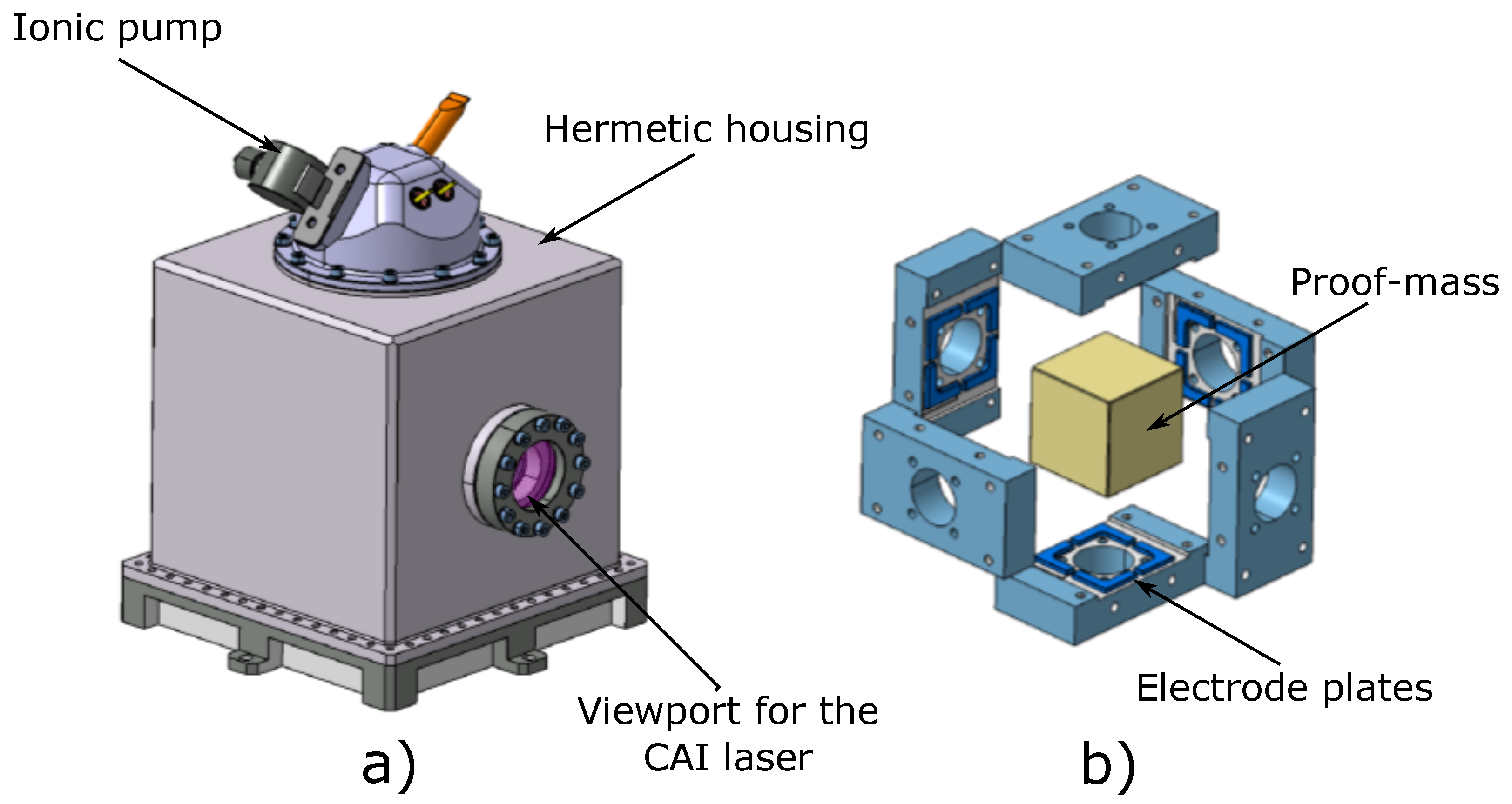
Remotesensing 14 03273 g027
Figure 28. (a) HybridSTAR electrostatic accelerometer. (b) HybridSTAR electrode plates with the cubic proof-mass.
Remotesensing 14 03273 g028
Figure 29. (a) HybridSTAR accelerometer performance on the along-track and cross-track axis. (b) HybridSTAR accelerometer performance on the radial axis.
Remotesensing 14 03273 g029
Figure 30. (a) Global hybrid instrument architecture. (b) Exploded view of the hybrid architecture.
Remotesensing 14 03273 g030
Figure 31. Temporal sequence describing the intermittent mode. The standard mode (up) allows acceleration measurements each T c . In the intermittent mode (bottom), the measurements are now only each n · T c . In this example, we take n = 4 . In between, the CAI is put in low power consumption mode (standby mode) allowing lowering the average electrical power consumption.
Remotesensing 14 03273 g031
Figure 32. Evolution of the CAI noise (QPN) due to intermittent operation for an interrogation time T = 2 s and a cycling time T c = 6 s in standard mode. The orange, purple, and green curves correspond, respectively, to an effective measurement cycling time of 6 s ( n = 1 ), 42 s ( n = 7 ), and 402 s ( n = 67 ).
Remotesensing 14 03273 g032
Table 1. Main characteristics of the last flying space EAs in CHAMP, GOCE, and GRACE-FO and the foreseen EAs for NGGM, the future ESA mission. For CHAMP, the mass and power consumption do not take into account the interface and control unit (ICU). USA and LSA stand, respectively, for ultra-sensitive axis and less-sensitive axis. For instance, in GRACE-FO, the USAs are the along-track and radial axes and the LSA is the cross-track axis.
EASpace Missions
CharacteristicsCHAMPGOCEGRACE-FONGGM
PM mass (g)7232072507
GAP USA ( μ m)75299175300
GAP LSA ( μ m)603260300
Meas. range USA [m·s 2 ] ± 10 4 ± 6 × 10 6 ± 7 × 10 5 ± 10 5
Meas. range LSA [m·s 2 ] ± 10 4 ± 5 × 10 4 ± 6 × 10 4 ± 10 5
Noise floor USA [m·s 2 ·Hz 1 / 2 ] 2 × 10 9 2 × 10 12 10 10 3 × 10 12
Noise floor LSA [m·s 2 ·Hz 1 / 2 ] 2 × 10 9 2 × 10 10 10 9 3 × 10 12
Total Mass [kg] (w. elec.)10 (w/o ICU)91115
Total Elec. Cons. [W]2 (w/o ICU)91115
Total Volume [L]13 (w/o ICU)111416
Table 2. Accelerometer parameters for simulations.
ParameterValueUnit
CAI Noise levelCase 14 × 10 8 m· s 2 ·Hz 1 / 2
Case 21 × 10 9
Case 31 × 10 10
Case 41 × 10 11
EA corner frequency 0.3mHz
1
3
EA low-frequency noise slope 1 / f -
1 / f 2
1 / f 3
Table 3. CAI parameters for scale factor uncertainty estimations. σ i refers to the uncertainty on the parameter i.
Parameters k e f f 1.6 × 10 7 m 1 τ R = 50 μ s T = 1 s Ω e f f = π / ( 2 τ R )
Uncertainty σ k e f f / k e f f = 10 9 σ τ R = 10 ns σ T = 10 ns σ Ω e f f / Ω e f f = 10 2
Table 4. Estimation of main errors coming from the coupling of the atomic source kinematics with the satellite rotation and the Earth gravity gradient. The estimations with rotation compensation are given considering a satellite rotation compensation with a residual at a level of 100 nrad/s.
Acc. Stab.Acc. Stab.Acc. Stab
Inertial Termswithout rot. Comp.with rot. Comp.with rot. Comp.
Around YAround Y and Z
± m · s 2 ± m · s 2 ± m · s 2
2 · Ω y · v z 2.3 × 10 6 2 × 10 10 2 × 10 10
2 · Ω z · v y 2 × 10 7 2 × 10 7 2 × 10 10
Ω y 2 · x 2.7 × 10 10 2 × 10 18 2 × 10 18
Ω ˙ y · z 2 × 10 10 2 × 10 10 2 × 10 10
Ω ˙ z · y 2 × 10 10 2 × 10 10 2 × 10 10
Γ x x · v x · T 3 × 10 9 3 × 10 9
Γ x x · x 6 × 10 10 6 × 10 10
Table 5. Assumptions on CAI atomic source parameters and satellite rotation parameters. δ i refers to the amplitude of variation impacting parameter i.
x , y , z = 0 v x , y , z = 0 Ω y = 1.16 mrad/s Ω x , z = 0.1 mrad/s (max)
δ x , y , z = ± 200 μ m δ v x , v y , v z = ± 1 mm/s Ω ˙ = 10 6 rad·s 2 (max, all axes)
Table 6. Size, weight, and power budget for the hybrid instrument. Note that the CAI budget for the electronics, laser, and microwave system was extrapolated by taking into account the PHARAO’s flight model budget [87,88].
Physics PackageElectronics/Laser/MWWhole Instrument
SizeWeightSizeWeightPowerSizeWeightPower
EA7 L6 kg9 L6 kg45 W16 L12 kg45 W
CAI36 L24 kg57 L39 kg100 W93 L63 kg100 W
Hybrid43 L30 kg66 L45 kg145 W109 L75 kg145 W
Publisher’s Note: MDPI stays neutral with regard to jurisdictional claims in published maps and institutional affiliations.

