Optimizing Local Alignment along the Seamline for Parallax-Tolerant Orthoimage Mosaicking

Abstract

Orthoimage mosaicking with obvious parallax caused by geometric misalignment is a challenging problem in the field of remote sensing. Because the obvious objects are not included in the digital terrain model (DTM), large parallax exists in these objects. A common strategy is to search an optimal seamline between orthoimages, avoiding the majority of obvious objects. However, stitching artifacts may remain because (1) the seamline may still cross several obvious objects and (2) the orthoimages may not be precisely aligned in geometry when the accuracy of the DTM is low. While applying general image warping methods to orthoimages can improve the local geometric consistency of adjacent images, these methods usually significantly modify the geometric properties of orthophoto maps. To the best of our knowledge, no approach has been proposed in the field of remote sensing to solve the problem of local geometric misalignments after orthoimage mosaicking with obvious parallax. In this paper, we creatively propose a method to optimize local alignment along the seamline after seamline detection. It consists of the following main processes. First, we locate regions with geometric misalignments along the seamline based on the similarity measure. Second, for any one region, we find one-dimensional (1D) feature matches along the seamline using a semi-global matching approach. The deformation vectors are calculated for these matches. Third, these deformation vectors are robustly and smoothly propagated into the buffer region centered on the seamline by minimizing the associated energy function. Finally, we directly warp the orthoimages to eliminate the local parallax under the guidance of dense deformation vectors. The experimental results on several groups of orthoimages show that our proposed approach is capable of eliminating the local parallax existing in the seamline while preserving most geometric properties of digital orthophoto maps, and that it outperforms state-of-the-art approaches in terms of both visual quality and quantitative metrics.

1. Introduction

Digital orthophoto maps (DOMs) are one of the most widely used products in the field of remote sensing, because they can provide both rich texture information of images and accurate geometric properties of maps [1]. Nowadays, DOMs have been popularly used in land cover segmentation [2,3], agricultural monitoring [4], and disaster management [5]. However, because the covered region of a single orthoimage is limited, it is necessary to stitch multiple orthoimages into one single composite image as seamlessly as possible in order to generate a large-scale DOM. Thus, image mosaicking is a key technology for producing seamless DOMs. Image mosaicking is a classical and important research topic in the fields of remote sensing [6] and computer vision [7]. In general, there are two key problems that need to be solved in the process of image mosaicking. The first problem is that there are large color differences between adjacent orthoimages due to different illumination and exposure settings. This problem can be solved using a color correction [8,9,10,11,12,13] or image blending approach [14,15]. The second problem is that geometric misalignments exist between adjacent images, especially for orthoimages. In general, orthoimages are generated from the satellite or aerial optical images using the process of orthorectification. In this paper, both satellite and aerial images are treated as remotely sensed images. Because the obvious objects are usually not included in the digital terrain model (DTM) which is applied to register normal remotely sensed images into orthoimages, the geometric position of the same obvious objects may be different in adjacent images. In this paper, our work focuses on solving the problem of parallax-tolerant orthoimage mosaicking.

A common strategy to solve the problem of geometric misalignment is to search for an optimal seamline between adjacent images, avoiding the objects with obvious parallax [16]. To date, many optimal seamline detection approaches [17,18,19,20,21,22,23,24,25] have been proposed for orthoimage mosaicking. In most of cases, these approaches can successfully avoid crossing the regions with large parallax and avoid the appearance of artifacts caused by geometric misalignments. However, stitching artifacts may appear along the seamline. One reason for this is that the seamline may cross several obvious objects with large parallax. Another reason is that if the accuracy of the DTM is not high enough, the orthoimages may not be precisely aligned in geometry. In this condition, although the seamline avoids crossing all obvious objects, artifacts may remain. Therefore, seamline detection methods cannot completely avoid the appearance of stitching artifacts caused by geometric misalignments. In order to further eliminate stitching artifacts, image warping needs to be performed after optimal seamline detection.

It has to be mentioned that in general image stitching tasks, various types of image warping methods [26,27,28,29] have been proposed to solve geometric misalignments. These methods generally divide the image into multiple regions and estimate the local transformation for each region by minimizing the feature matching error. However, these methods cannot be directly applied to orthoimage mosaicking tasks. Because the pixel locations of orthoimage correspond to real geographic coordinates, orthoimage mosaicking needs to preserve the original geometric properties of the image as much as possible, while these warping methods tend to significantly modify the geometric properties of the entire image.

Considering the above reasons, we propose a novel local alignment optimization method for parallax-tolerant orthoimage mosaicking. After detecting the optimal seamline, the core idea of the proposed method is to find the regions with geometric misalignments along the seamline and eliminate the residual artifacts by warping the image locally. The optimization effect of the proposed method is shown in Figure 1. These two examples represent two situations: the misalignments in Figure 1a are caused by the seamline crossing the building, and the misalignments in Figure 1b are due to insufficient DTM accuracy. It can be seen that after the proposed local alignment optimization process, the geometric misalignments have been well eliminated. In this way, geometric misalignments can be eliminated while preserving the geometric properties of the images as much as possible. In our proposed method, we first compute the similarity of the neighborhood of each point on the seamline. The lower the similarity score, the greater the difference between the images in this area, and the more likely it is that there are geometric misalignments. After locating regions where misalignments may exist, local alignment optimization is performed for each region in turn. Specifically, according to the semi-global matching (SGM) approach [30], we find one-dimensional (1D) feature matches along the seamline and compute the corresponding deformation vectors. It should be noted that other 1D feature matching methods [31,32] can be integrated into our framework in order to find the matches. Then, the associated energy function is constructed and minimized to smoothly propagate these deformation vectors to the seamline-centered buffer region. Finally, we warp the orthoimage based on the dense deformation vectors. Furthermore, the local alignment optimization for each region can be processed in parallel. Experimental results on orthoimage datasets show that our proposed method outperforms the current representative methods in both visual quality and quantitative metrics.

The rest of the paper is structured as follows. Section 2 provides an overview of related works. In Section 3, the proposed local alignment optimization algorithm is elaborated. The experiments are presented in Section 4. Finally, conclusions are drawn in Section 5.

2. Related Work

Related research is introduced from two aspects: optimal seamline detection and image warping methods.

2.1. Optimal Seamline Detection

Optimal seamline detection methods search for the seamlines in overlap regions between images, where their intensity or gradient differences are minimal, especially avoiding crossing the obvious objects with large parallax. Typically, these methods formulate the optimal seamline detection problem as an energy optimization problem, and they can be divided into two steps. In the first step, a cost energy function is designed to represent the differences between adjacent images using the pixel information [17,18,19], object [20,21,25], and auxiliary data [22,23,24]. The major differences between different approaches are that their cost functions are defined with the use of different information or features. In the second step, an optimal seamline with the minimal cost is detected from the cost map using snake model [33], dynamic programming [34], Dijkstra’s algorithm [35], and graph cuts [36]. The major issues with the optimal seamline detection methods are focused on how to define the energy function reasonably and how to find the optimal solution efficiently. According to the information used in energy function construction, we briefly review recently proposed optimal seamline detection methods.

When designing the loss energy function, the most straightforward strategy is to build it based on image pixel information, such as color, gradient, and texture. Kerschner [17] proposed an automatic seamline detection method using twin snakes. The energy function designed by this method includes information such as hue, intensity, and gradient to express color similarity and texture similarity. Finally the twin snakes were used to delineate the proper seamline with maximum similarity. Yu et al. [18] calculated the loss function based on three types of information: a pixel-based similarity measurement defined by color, texture, and edge intensities; a region-based saliency map based on a human attention model; and the distance between the pixel and the nadir points of the dataset. Then, the position of the seamline is tracked with a dynamic programming algorithm. Li et al. [19] proposed a multi-frame joint optimization strategy to effectively find optimal seamlines from multiple aligned images. In this method, color intensities, gradient magnitudes, and texture complexity are integrated into the energy function. Dai et al. [37] presented a deep learning framework named Edge Guided Composition Network. This method regresses the blending weights of the input images to seamlessly produce the stitched image.

The parallax of obvious objects in the orthoimage is large, while the parallax of road and ground is small. Considering the regionality of parallax distribution, many methods have considered segmentation-based region information when constructing energy equations. Wang et al. [20] proposed a seamline detection algorithm based on watershed segmentation. This algorithm first obtains the objects using regional adaptive marker-based watershed segmentation. Then, the object difference is calculated and the objects through which the seamlines pass are determined by minimizing the maximum object cost. Finally, pixel-level optimization is performed using Dijkstra’s algorithm to determine the final seamlines. Pang et al. [21] proposed a new semi-global matching (SGM)-based method to guide seamline detection. In their method, the SGM algorithm is applied to the overlap area to obtain the corresponding pixel-wise disparity. Then, regions with parallax less than a predefined threshold are identified as non-obstacle regions. In the non-obstacle regions, the Hilditch thinning algorithm is used to obtain the skeleton line, followed by Dijkstra’s algorithm to search for the optimal path on the skeleton network. Li et al. [38] applied the semantic segmentation results generated by a deep learning-based method to guide optimal seamline detection. Yuan et al. [25] proposed a seamline detection method based on a road probability map. This method obtains a road probability map with the D-LinkNet neural network. The preferred road areas (PRAs) are determined by binarizing the road probability map of the overlapping area. Then, the final seamlines are determined by Dijkstra’s algorithm at the pixel level.

In addition to pixel and object information, auxiliary data are sometimes used to aid in avoiding crossing the obvious objects in the orthoimage. Chen et al. [22] proposed to guide a seamline toward the low area on the basis of the elevation information in the digital surface model (DSM). As the elevation of DSM is not completely synchronous with DOM, an orthoimage elevation synchronous model (OESM) is derived and introduced. The initial path network is obtained on the basis of OESM, and Dijkstra’s algorithm is used to determine the path with minimal cost. Wang et al. [23] presented a novel seamline detection approach based on vector building maps. This approach traces the centerlines between vector buildings to generate the candidate seams. The candidate seams are then refined by considering their surrounding pixels to minimize the visual transition between the images to be mosaicked. Zheng et al. [24] proposed a weighted ${\mathrm{A}}^{*}$ algorithm for seamline detection. The edge diagram is first generated by detecting large height gradients in the DSM data. Then, a weighted ${\mathrm{A}}^{*}$ algorithm is proposed to search for an optimal path from the starting to the ending point of each seamline while avoiding high objects.

From review of the above-mentioned optimal seamline detection methods, it can be seen that these methods generate seamless composite image by avoiding crossing obvious objects with large parallax. Sometimes, when it is unavoidable to cross obvious objects, such methods cannot handle geometric misalignments.

2.2. Image Warping Methods

In image stitching, images are transformed into the same coordinate system by various image warping methods. Assuming that all input images are captured in rotation or that the scene can be approximated as a plane, the transformation between images can be represented by a global homography matrix [26]. If these two requirements are not met, visible artifacts caused by parallax will appear in the resulting mosaic. Therefore, many image warping methods have been proposed to reduce the local geometric misalignment, thereby improving the visual effect of the mosaic.

Adaptive warping methods typically handle images with parallax by estimating multiple local transformations. Gao et al. [39] proposed a dual-homography method that blends the two homographies in the alignment procedure to produce a more seamless image when the scene contains two dominant planes. Lin et al. [40] estimated a smoothly varying affine field to flexibly handle parallax with a pre-computed global affine transform as a constraint. Zaragoza et al. [27] proposed a new image warping method called Moving Direct Linear Transform (Moving DLT). This method divides the input image into regular grid cells and estimates the best homography for each cell. All feature points participate in the homography estimation of the cell, and the weight of any feature point is inversely proportional to its distance from the target cell. Li et al. [41] proposed a parallax-tolerant image stitching method based on robust elastic warping. In their method, the analytical warping functions are constructed from matching points to eliminate the parallax errors.

Adaptive warping methods can align overlapping regions between two images well, although non-overlapping regions usually exhibit severe perspective distortion. Therefore, Shape-Preserving warping methods have been proposed to alleviate perspective distortion in non-overlapping regions between two images. Chang et al. [28] proposed a Shape-Preserving Half-Perspective (SPHP) warping method which is a spatial combination of a projective transformation and a similarity transformation. This method smoothly extrapolates the projective transformation in the overlapping regions into the similarity transformation in non-overlapping regions. Lin et al. [42] proposed a warping model that combines local homography and global similarity to generate natural-looking results.

Unlike adaptive warping methods, the goal of seam-driven warping methods is not to minimize the error of feature matching, but rather to find a deformation scheme that minimizes the misalignment at the seam. Gao et al. [29] proposed a seam-driven image warping strategy that evaluates the quality of estimated transformations based on the visual quality of seam cuts. Zhang and Liu [43] proposed a hybrid alignment model to handle large parallax and local distortion. This method uses the seam cost as the quality metric to estimate the optimal homography, and further uses content-preserving warping (CPW) [44] to locally refine the alignment. Although seam-driven methods can produce visually pleasing mosaic results, they may not guarantee geometric accuracy over the entire image.

The above feature-based image warping methods rely on the quality of feature matching, and are prone to failure when stitching images with weak texture or low resolution. In recent years, several deep learning-based methods [45,46,47,48] have been proposed to solve the image warping problem. Zhang et al. [46] proposed a content-aware unsupervised network which selects reliable regions for homography estimation by learning an outlier mask. Nie et al. [48] proposed an unsupervised deep image stitching framework consisting of two stages: unsupervised coarse image alignment and unsupervised image reconstruction. Specifically, the reconstruction network consists of a deformation branch that can learn deformation rules of image stitching and a refined branch that enhances the resolution.

Although image warping methods are more flexible and effective in improving geometric alignment, these methods usually significantly modify the geometric position of the image. However, orthoimages have the characteristic that their pixel positions correspond to real geographic coordinates. This requires that the original geometric properties be preserved as much as possible when deforming the local image.

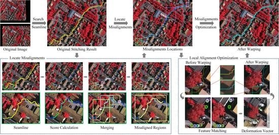
3. The Proposed Local Alignment Optimization Approach

Given two adjacent orthoimages $I_l$ and $I_r$ (or multiple images), we attempt to generate a larger composite image that is as seamless as possible. The current mainstream approach is to find the optimal seamline between adjacent images in order to bypass obvious objects. However, sometimes the seamline inevitably crosses several obvious objects, or DTM is not accurate enough to align the orthoimages precisely. As a result, the composite image exhibits artifacts near the seamline. To solve this problem, we creatively propose a local alignment optimization approach for parallax-tolerant orthoimage mosaicking. The workflow of the proposed local alignment optimization approach is shown in Figure 2.

Suppose the optimal seamline has been detected for these two adjacent images, denoted as $L={\left\{p_i\right\}}_{i=0}^N$. Where $p_i$ represents the i-th point on seamline L, N is the number of points. In this paper, we directly apply our previous work [19] to detect the seamline between two images. After detecting the seamline, the first step of our approach is to locate the regions with geometric misalignments along the seamline. For each point on the seamline, the similarity between the left and right images $I_l$, $I_r$ is calculated within its neighborhood. It is generally believed that the lower the similarity, the more likely there will be geometric misalignments. After detecting possible regions of geometric misalignments, we can process each region independently. This is done for three reasons. First, orthoimages are usually large, and processing each region independently helps reduce the memory requirement of the algorithm. Second, performing SGM on the entire seamline is time-consuming and prone to mismatching, while performing SGM on the local seamline has higher efficiency and accuracy. Third, processing each local region independently helps preserve the geometric properties of other regions of the orthoimage.

For any local region, we perform local alignment optimization to eliminate the geometric misalignments existing near the seamline. Specifically, we first detect 1D feature matches on seamlines based on the SGM method. Compared with the general brute force matching method, the SGM method is more robust. The brute force matching only considers the feature points themselves, while SGM adds a smoothness constraint by penalizing the neighborhood disparity changes at each feature point location. Then, we compute the corresponding deformation vectors from the matching points and build buffers centered on the seamline. By constructing and minimizing the energy function, we smoothly propagate the deformation vectors to the rest of the buffer region. Finally, we warp the orthoimages guided by the deformation vectors.

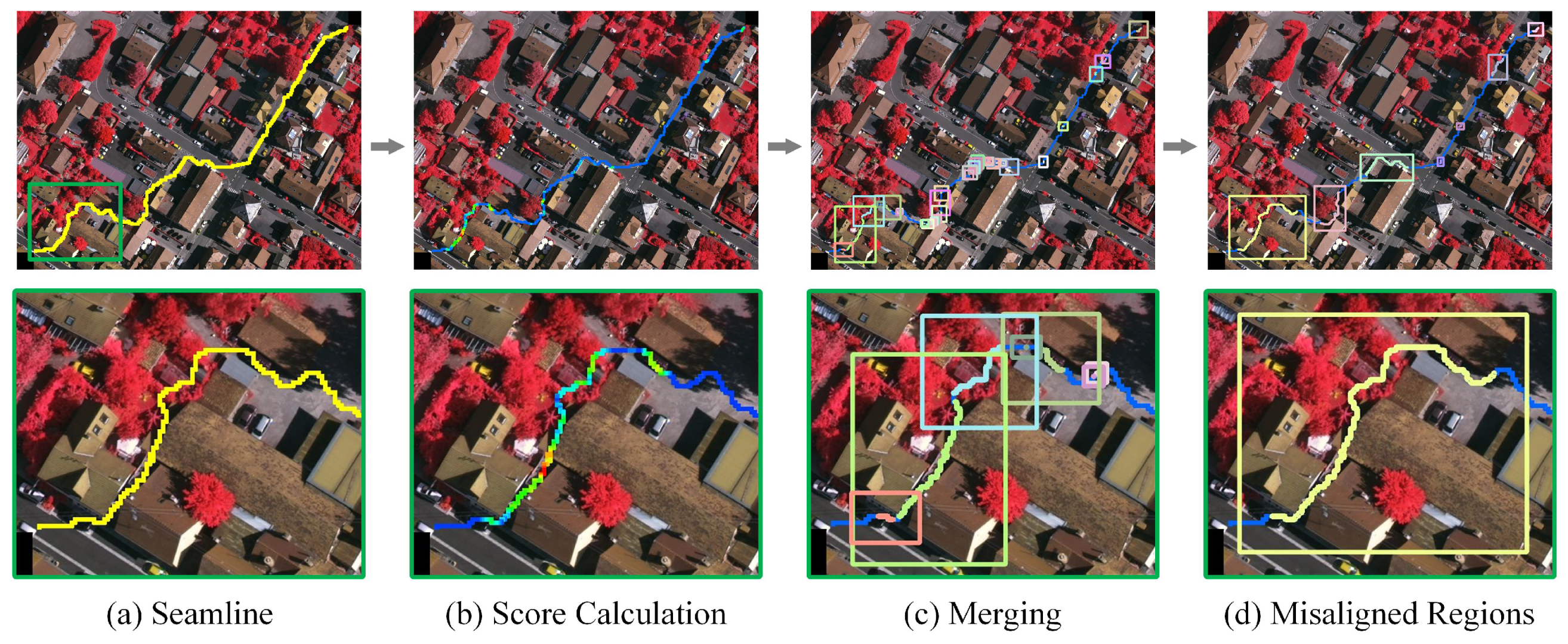
3.1. Misalignment Location

After detecting the optimal seamline, we actually rely on the matching feature points to guide the final local image warping. However, feature matching on the entire seamline is not only inefficient, it is prone to false matching. Therefore, we first detect regions of possible geometric misalignments along the seamline. Then, local alignment optimization can be performed independently for each region. Moreover, our strategy is conducive to the parallel optimization of the algorithm. The calculation process of a misaligned location is shown in Figure 3.

First, misalignment scores need to be calculated for the neighborhoods of points on the seamline. Assuming that the masks of $I_l$ and $I_r$ are denoted as $M_l$ and $M_r$, the overlapping region of the two images can be denoted as $M_o=M_l\cap M_r$. For each point $p_i$ on the seamline L, take a block centered on $p_i$, which is denoted as $M_b^i$. Then, according to the masks, two corresponding sub-image blocks can be obtained, denoted $B_l^i=I_l(M_o\cap M_b^i)$ and $B_r^i=I_r(M_o\cap M_b^i)$. In general, for any point $p_i$, the misalignment score of its neighborhood is calculated as follows:

$$s_i=\left\{\begin{array}{cc}{\displaystyle 1-\frac{\mathrm{SSIM}(B_l^i,B_r^i)}{T_s},}\hfill & \mathrm{if}\mathrm{SSIM}(B_l^i,B_r^i)<T_s,\hfill \\ 0,\hfill & \mathrm{if}\mathrm{SSIM}(B_l^i,B_r^i)\ge T_s,\hfill \end{array}\right.$$

(1)

where $\mathrm{SSIM}(B_l^i,B_r^i)$ is the SSIM between the image blocks $B_l^i$ and $B_r^i$, while $T_s$ is the threshold. When the calculated value of SSIM is less than the threshold, we consider that there may be geometric misalignments at the point. Specifically, SSIM is calculated as follows (for convenience of expression, $B_l^i$ and $B_r^i$ are replaced by x and y):

$${\displaystyle \mathrm{SSIM}(x,y)=\frac{(2{\mu }_x{\mu }_y+c_1)(2{\sigma }_{xy}+c_2)}{({\mu }_x^2+{\mu }_y^2+c_1)({\sigma }_x^2+{\sigma }_y^2+c_2)},}$$

(2)

where ${\mu }_x$ and ${\mu }_y$ are the mean values of the block x and y, ${\sigma }_x$ and ${\sigma }_y$ are the variances, ${\sigma }_{xy}$ is the covariance of x and y, and $c_1$ and $c_2$ are two constants.

All misalignment scores can be expressed as $S={\left\{s_i\right\}}_{i=0}^N$. As shown in Figure 3b, the graduated color from blue to red is used to represent the score from low to high. Points with a score of 0 are considered to have no geometric misalignment; the higher the score, the more likely there is to be a geometric misalignment. Points with $s_i\ne 0$ are concatenated to form local seamlines, denoted as

$$\mathcal{R}={\left\{R_j\right\}}_{j=0}^{N_r},R_j={\left\{p_i\right\}}_{i=a_j}^{b_j},$$

(3)

where $N_r$ is the number of local seamlines and $a_j$ and $b_j$ are the start and end indices of the j-th local seamline.

When warping an image, the deformation is propagated to the surrounding buffer. Therefore, local regions with close distances should be merged for simultaneous optimization. Specifically, an outer rectangle is constructed with $R_j$ as the center and expanded outward by a certain width. The outer rectangles of different local regions are represented by different colors in Figure 3c. The expanded width is positively correlated with the maximum misalignment score on the local seamline $R_j$, expressed as $w_{rect}=100\times s_{max}$. As shown in Figure 3c, the affected area of several local seamlines is different in size. If any two rectangles overlap, the corresponding local seamlines will be merged. Finally, we obtain a set of merged local seamlines, denoted as $\mathcal{R}={\left\{R_j\right\}}_{j=0}^{N_m}$, where $N_m$ is the number of local seamlines after merging. Figure 3d shows the local seamlines after merging the regions of possible geometric misalignment.

During the misalignment location process, a threshold, $T_s$, is introduced for segmentation, as described in Equation (1). The influence of this parameter on the algorithm is mainly as follows: (1) if a higher value is set, the local region may be too large and even cannot be divided; (2) if the value is too small, the region with geometric misalignment may be incorrectly judged to be aligned. In this paper, the threshold is set to the average of all SSIM values on the seamline. Figure 4 shows the misalignment location results with different threshold values.

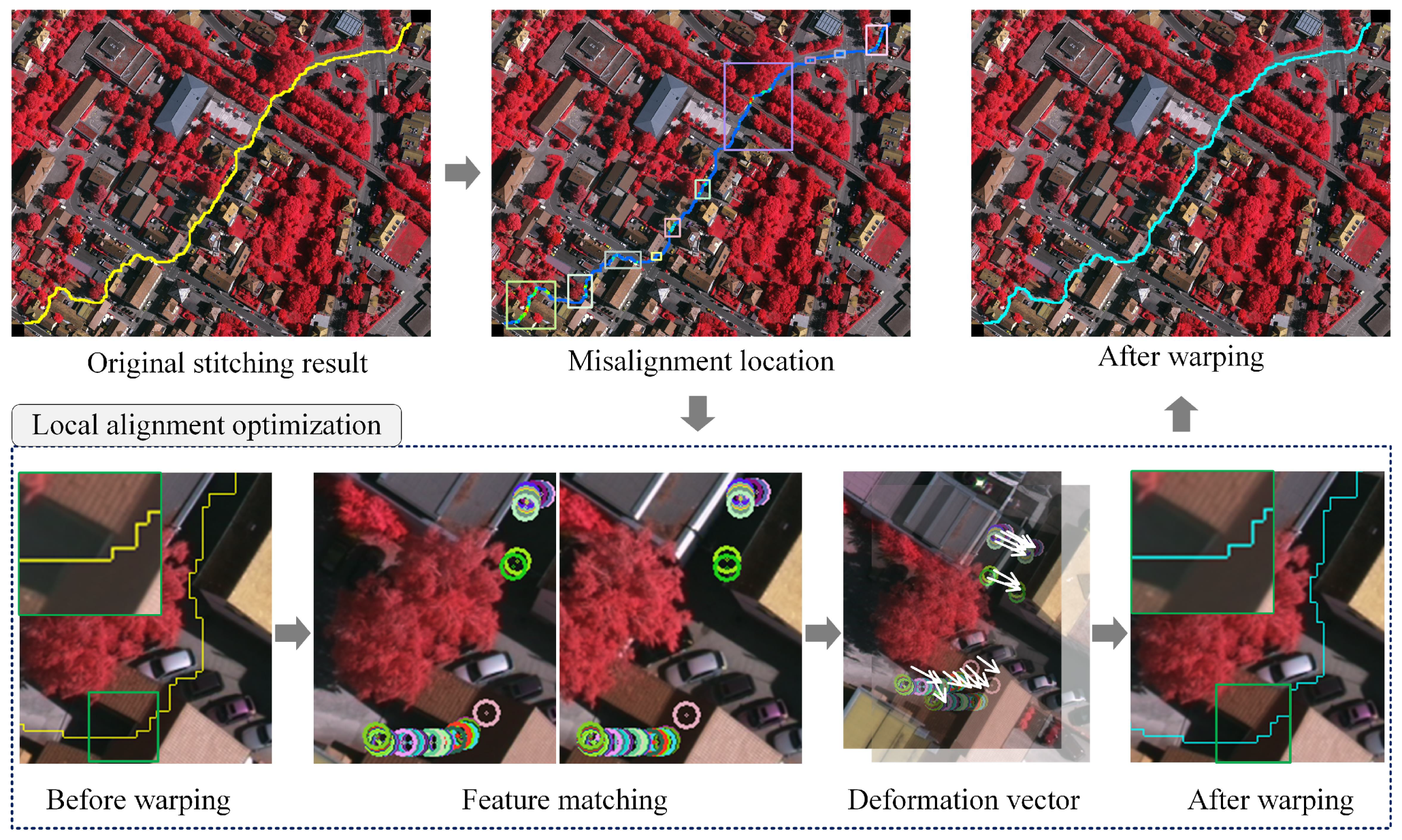
3.2. Local Alignment Optimization

After locating regions where there may be geometric misalignments, we process each local region in turn. For a local region $R={\left\{p_i\right\}}_{i=a}^b$, we first perform 1D feature matching on the local seamline according to the semi-global matching (SGM) approach [30]. Then, the deformation vectors are calculated for these feature matches. After that, the deformation vectors are smoothly propagated to the seamline-centered buffer by minimizing the associated energy function. Finally, the image is warped under the guidance of the deformation vectors.

3.2.1. Feature Matching

Each point on the local seamline $R={\left\{p_i\right\}}_{i=a}^b$ is regarded as a feature point. Denote the feature points of $I_l$ and $I_r$ as $F_l={\left\{f_{l,i}\right\}}_{i=a}^b$ and $F_r={\left\{f_{r,i}\right\}}_{i=a}^b$, respectively. The histogram of the oriented gradient (HOG) descriptors [49] of the feature points are calculated first; then, the SGM algorithm is applied to search for the feature matching results. Finally, a consistency check is performed. The specific steps are as follows.

In this paper, the gradient directions are equally divided into K intervals. Therefore, the calculated HOG descriptor can be expressed as $H={\left\{h_k\right\}}_{k=1}^K$. The HOG descriptor set of $F_l$ and $F_r$ is denoted as ${\mathcal{H}}_l={\left\{H_{l,i}\right\}}_{i=a}^b$ and ${\mathcal{H}}_r={\left\{H_{r,i}\right\}}_{i=a}^b$. Because the feature points are distributed on the seamline, there is a correlation between adjacent points. Therefore, the feature matching results can be searched according to the SGM algorithm. The SGM algorithm is mainly divided into four steps: matching cost calculation, cost aggregation, disparity computation, and disparity refinement. First, we set the disparity search range, $D=[d_{min},d_{max}]$. We introduce a cost space C of size $N_R\times D$, where $N_R=b-a+1$ is the number of points in the local seamline R. Each element in C represents the matching cost value of each feature point in $F_l$ under each parallax within the parallax range. The matching cost calculation requires us to fill C by calculating the correlation between feature points. For the i-th feature point in $F_l$, the matching cost between it and the feature point with disparity d in $F_r$ is calculated as follows. Let $j=i+d$; then:

$$\mathcal{M}(i,j)=\sqrt{{\displaystyle 1-\frac{\mathrm{Sum}(H_{l,i},H_{r,j})}{\sqrt{\mathrm{Sum}\left(H_{l,i}\right)\times \mathrm{Sum}\left(H_{r,j}\right)}}}},$$

(4)

where $\mathrm{Sum}\left(H_{l,i}\right)$ and $\mathrm{Sum}\left(H_{r,j}\right)$ are the sum of the HOG descriptors, expressed as $\mathrm{Sum}\left(H\right)={\sum }_{k=1}^K{h}^k$. $\mathrm{Sum}(H_{l,i},H_{r,j})$ expresses the correlation between two descriptors, calculated as follows:

$$\mathrm{Sum}(H_{l,i},H_{r,j})=\sum _{k=1}^K\sqrt{h_{l,i}^k\times h_{r,j}^k},$$

(5)

After computing all elements of the cost space C, we obtain the matching cost of each feature point within the disparity range. However, point-by-point matching is not precise enough. To prevent noise interference, cost aggregation is required. That is, a smoothness constraint is added by penalizing the neighborhood disparity variation of each feature point location. We aggregate in the forward and reverse directions, respectively, and the final cost aggregate value is the sum of the aggregate values of all paths. Refer to [30] for details on cost aggregation.

Finally, we can find all matches between two sets of feature points by minimizing the whole matching costs using the optimization method presented in SGM [30]. For each feature point, we can obtain the 1D disparity vector $D_l$. That is, if the disparity of the i-th feature point $f_{l,i}$ is d, then its matching point is the $i+d$-th feature point $f_{r,i+d}$. In addition, to further filter the outliers and refine the matches, we perform a consistency check. The right image is used as the base image for matching, and the disparity vector $D_r$ is obtained. If the corresponding disparities of $D_l$ and $D_r$ are inconsistent, it is regarded as invalid disparity. The disparity of $f_{l,i}$ is calculated as follows:

$$D_i=\left\{\begin{array}{cc}{D}_{l,i},\hfill & \mathrm{if}{D}_{l,i}+D_{r,j}=0,\hfill \\ D_{\mathrm{inv}},\hfill & \mathrm{otherwise}.\hfill \end{array}\right.$$

(6)

where $j=i+D_{l,i}$. Therefore, the set of matching points is represented as

$$P=\left\{(f_{l,i},f_{r,j})\right|i\in [a,b],j=i+D_i,D_i\ne D_{inv}\}.$$

(7)

3.2.2. Deformation Map

After obtaining the feature matching results, we calculate the corresponding deformation vector as follows:

$${\mathbf{v}}_{i,j}=f_{l,i}-f_{r,j},$$

(8)

where $(f_{l,i},f_{r,j})$ is a pair of matching points. The set of deformation vectors is denoted as $V=\left\{{\mathbf{v}}_{i,j}\right|(f_{l,i},f_{r,j})\in P\}$. When the modulus of the deformation vectors in the local region R is less than one pixel, the region is skipped without processing. Otherwise, we perform subsequent local alignment optimization. When warping the misaligned region, it should gradually transition to the surrounding area. Therefore, the size of the buffer is determined according to the size of the deformation vector, which is formulated as follow:

$$siz{e}_b=c_b\times \max \left(\right|V\left|\right),$$

(9)

where $\max (·)$ means the largest modulus in the deformation vector set V and $c_b$ is a coefficient. In our method, we set $c_b=30$. This means that a misalignment of one pixel will use a space of 30 pixels to transition. In this way, we can avoid the appearance of artifacts after the local image warping.

To warp the local buffer region, we need to know the deformation vectors of all pixels in this area. In the buffer region, the deformation vectors of the matching points are known. In addition, to avoid destroying the geometric information of the whole orthoimage we set the deformation vectors of the buffer boundary to zero. Specifically, the image content outside of the local buffer area will not be modified. As shown in Figure 5, according to the known information and smoothness constraints, the energy equation is constructed and minimized to obtain the deformation vectors of all points in the buffer.

Let $\mathbf{X}={\left\{{\mathbf{x}}_k\right\}}_{k=1}^{N_B}$ denote all the deformation vectors to be solved in the buffer region. $N_B$ is the number of points in the buffer. The energy equation is defined as

$$\begin{array}{cc}\hfill E& =\sum _{{\mathbf{x}}_k\in V}\parallel {\mathbf{x}}_k-{\mathbf{v}}_k{\parallel }_2+\sum _{{\mathbf{x}}_k\in B}{\parallel {\mathbf{x}}_k-0\parallel }_2\hfill \\ \hfill & +\sum _{{\mathbf{x}}_k\notin V\cup B}{\parallel 4·{\mathbf{x}}_k-\sum _{{\mathbf{x}}_n\in N\left({\mathbf{x}}_k\right)}{\mathbf{x}}_n\parallel }_2.\hfill \end{array}$$

(10)

This energy function consists of three terms. The first term represents the matching point constraint, and ${\mathbf{v}}_k$ is the known deformation vector corresponding to the current position. Namely, for the matching points, the solved deformation vectors should be the same with the offsets between two points. The second term represents the boundary point constraint, where B is the set of boundary points. If the pixels belong to the boundaries of the buffer region, the corresponding deformation vectors should be 0. The last term is the smoothness constraint, which spreads the deformation vectors of the matching points smoothly by constraining the gradient of the current position to be as small as possible. $N\left({\mathbf{x}}_k\right)$ is the 4-neighborhood of ${\mathbf{x}}_k$. In our method, we solve for the deformation values in the horizontal and vertical directions separately. The above energy equation can be easily solved using the $Eigen$ library (http://eigen.tuxfamily.org, accessed on 15 May 2022).

After obtaining the deformation vectors for each pixel in the buffer, we warp the image according to the bilinear interpolation method. For details, please refer to our previous work [50]. In fact, for the pixels in the left and right images, we warp each by half the size of the deformation vector and in opposite directions. In this way, the matching points on the left and right images will be warped to the same position, as shown in Figure 5c.

4. Experimental Results and Discussion

We evaluated the performance of our proposed local alignment optimization method using three pairs of test images, namely, AERIAL-1, AERIAL-2, and SATELLITE-1. The first two sets are aerial images, and the third set consists of satellite images. Detailed descriptions of these three datasets are presented in

Table 1. The details of the three datasets used in our experiments.

	Spatial Resolution	Spectral Bands	Descriptions
AERIAL-1	0.1 m	IR-R-G	Small-sized buildings; many surrounding trees
AERIAL-2	0.2 m	R-G-B	Medium-sized buildings; dense residential area
SATELLITE-1	1 m	R-G-B	Suburb district; high speed road; woodland

. In order to compare the improvement effect of different methods on local misalignments, we used APAP [27], ELA [41], and our proposed method for local image warping respectively after detecting local misalignment regions. The warp results of APAP [27] and ELA [41] were obtained according to the source codes provided by the authors. Then, the warped images were combined according to the precomputed optimal seamline. The experiments were divided into two parts: the first part was a qualitative experiment which evaluated the proposed method by comparing the stitching results after local warping, while the second part calculated the structural similarity (SSIM) and geometric error (GE) for quantitative evaluation.

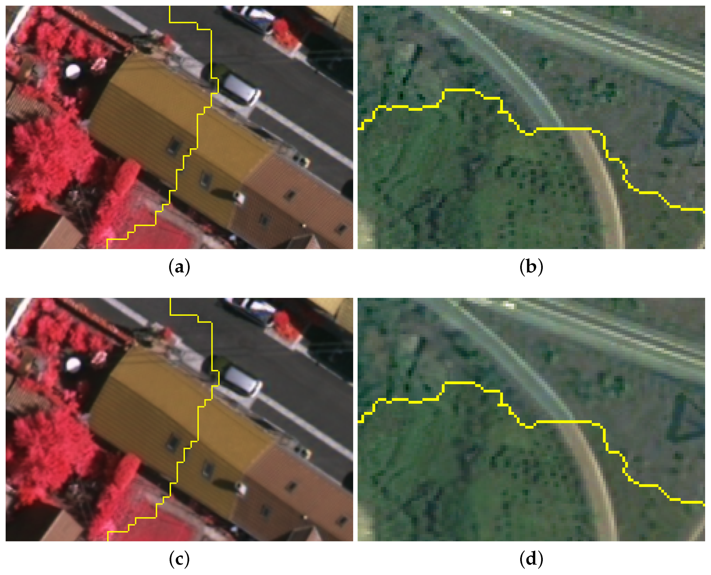
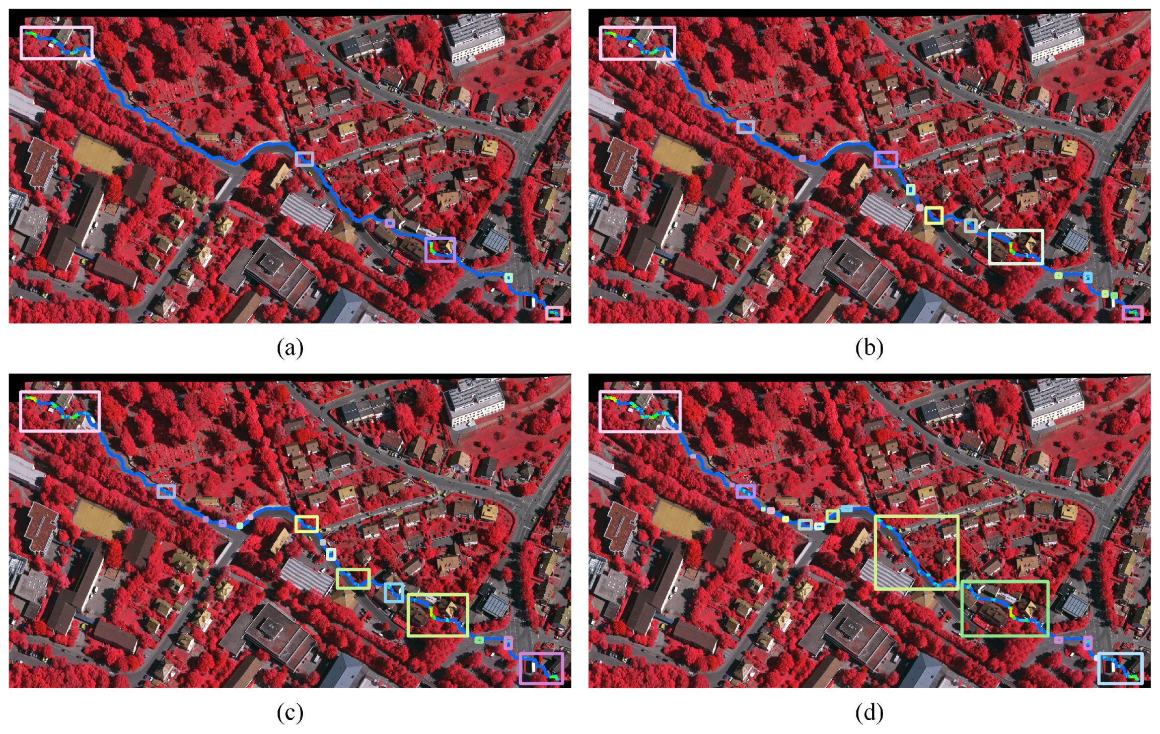
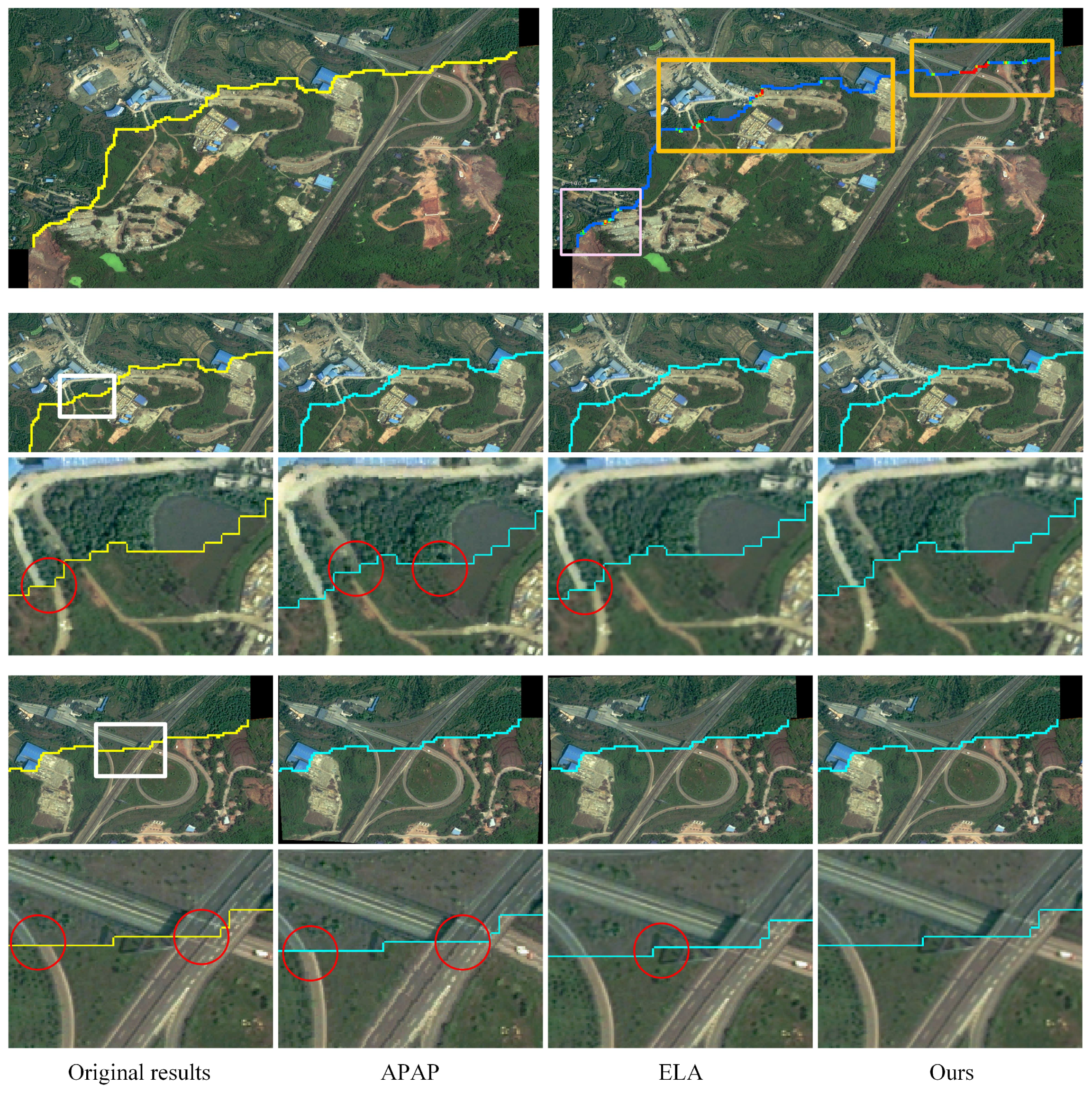
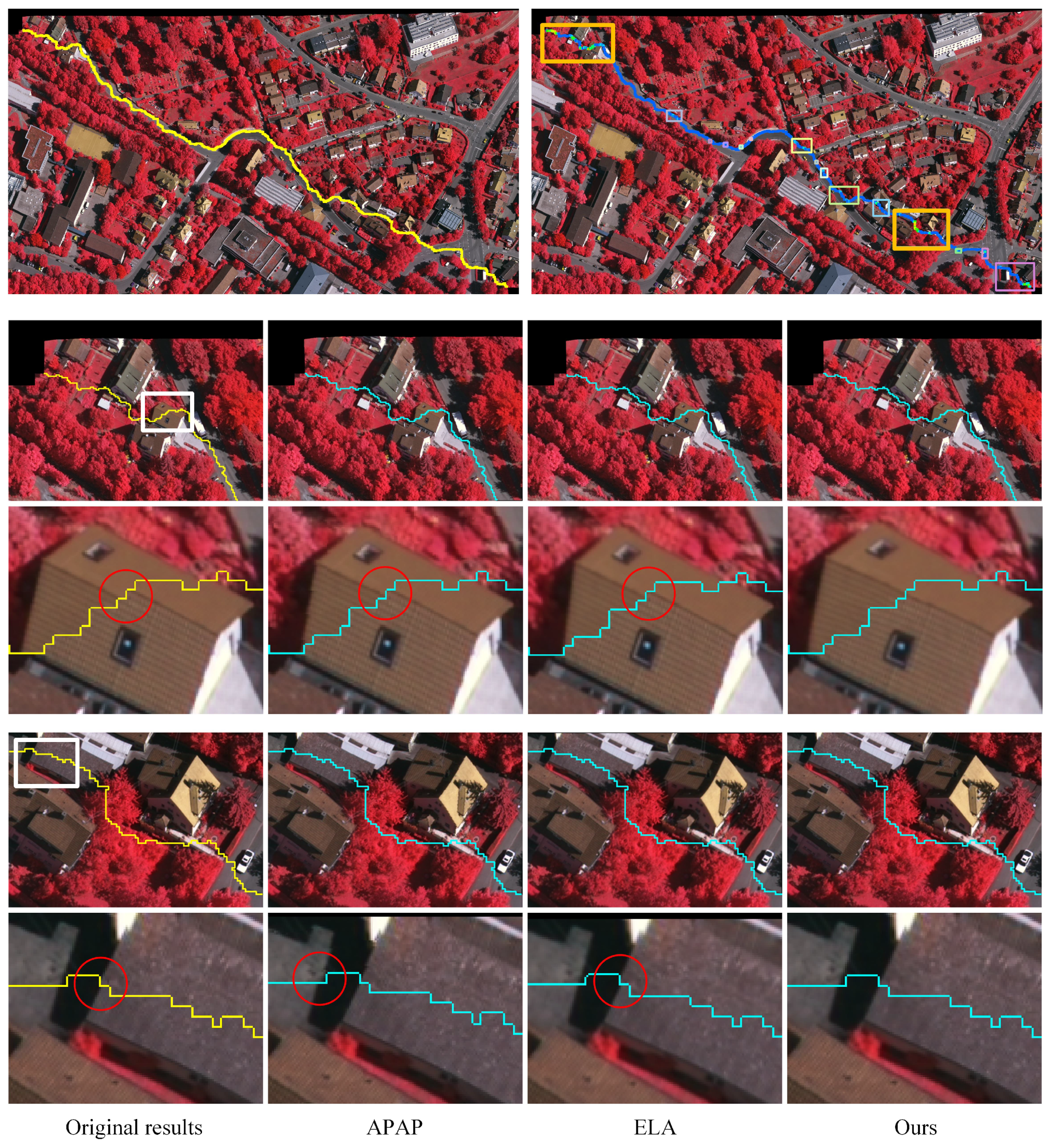
4.1. Qualitative Evaluation

We conducted qualitative evaluation experiments on three pairs of images. Figure 6 presents the warp results of the three methods on AERIAL-1. The first row presents the optimal seamline and the detected misaligned local regions. Due to space limitations, two regions marked by orange boxes were selected for presentation for each set of data. From the original stitching results presented in rows 3 and 5, it can be seen that when the seamline passes through obvious objects such as houses, there are obvious misalignments caused by parallax near the seamline. For the first enlarged region, the seamline runs continuously across the ridge and eaves. As indicated by the red circles in the third row, the misalignments in the results of APAP [27] and ELA [41] are alleviated, but still obvious. Both the two methods are local warping methods based on feature matching, and the warping effect relies on the guidance of feature matching. However when there is a large parallax, even if the feature matching is correct it cannot lead to a geometrically consistent stitching result. On the other hand, the proposed method only considers the geometric consistency on the seamline, and produces results with invisible geometric misalignments. For the second enlarged region, the seamline crosses the eave, although with less parallax. It can be seen that APAP [27] aligns the eave, but causes the shadow adjacent to it to be misaligned. The result of ELA [41] is not significantly improved compared to before optimization. Our method aligns the eave better without affecting nearby areas.

Figure 7 presents the warp results of the three methods on AERIAL-2. For the first region, as can be seen from the first image in the third row, there are large geometric misalignments around the seamline. This is because the seamline passes through the tall buildings. Especially where the red circles are marked, the large parallax causes the distance between the wall and the gray stripe to be different. Among the warp results, the results of APAP [27] are the worst visually. This method barely aligns the wall and gray strip, and causes them to bend and deform, destroying their original geometric character. ELA [41] and the proposed method look relatively better, but only align one of them: ELA [41] aligns the wall, and the proposed method aligns the gray strip. For the second region, the edge in the middle of the roof has a slight geometric misalignment. In the result using APAP [27], the geometric misalignment here is more serious, probably due to the deformation caused by the false matching in the nearby area. ELA [41] solves the problem of misalignment, but it causes the distortion of the image, making the straight eave become curved. The proposed method, on the other hand, obtains natural results with no apparent misalignment.

Figure 8 presents the warp results of the three methods on SATELLITE-1. This dataset consists of two satellite images. In addition, the features on the left image and right image differ greatly due to different shooting times. For the first region, as shown in the third row in Figure 8, the seamline crosses two paths and the lakeshore. It is easy to see that the geometrical misalignments are large and obvious. In the result using APAP [27], the path on the left is aligned, while the path on the right and the lakeshore are misaligned. Although ELA [41] successfully aligns the right path and the lakeshore, it fails to align the left path. In the result using our proposed method, the paths and the lakeshore are all well-aligned.

For the second region, the warp result of APAP [27] is relatively poor. There are obvious geometric misalignments in the longitudinal road and the curved road. The result of ELA [41] has a misalignment near the intersection. For this region, the proposed method again achieves the best result.

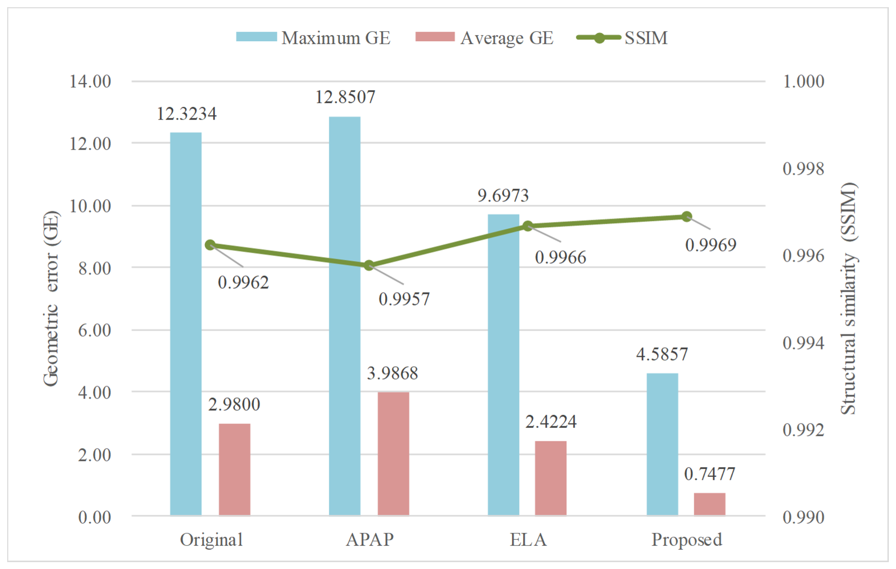
4.2. Quantitative Evaluation

In addition to the experiments described above, in order to convincingly illustrate the effectiveness and superiority of the proposed method we conducted quantitative evaluation experiments on these three pairs of images. Specifically, for any local region we calculated the geometric error (GE) of the warp results along the seamline based on feature matches, and calculated the corresponding maximum and average values. We calculated the structural similarity (SSIM) of the local regions near the seamline of the left and right images for reference. Lower values of GE and higher values of SSIM denote the better alignment results. For convenience, the averages of maximum GE, average GE and SSIM of the six local regions in three pairs of images were calculated for quantitative evaluation, as shown in Figure 9. For the original images that were registered but not locally warped, the maximum GE and average GE are 12.3234 and 2.9800, respectively, and the SSIM is 0.9962. APAP [27] and ELA [41] yield a maximum GE of 12.8507 and 9.6973, and average GE of 3.9868 and 2.4224, respectively. The proposed method achieves the minimum geometric errors, with a maximum GE of 4.5857 and the average GE of 0.7477. This proves that the proposed method performs better in local alignment optimization, and can effectively eliminate the local geometrical misalignments. For structural similarity, our proposed method again has the best score, followed by ELA [41] and APAP [27]. This shows that in the region near the seamline, the results generated by the proposed method have the best alignment effect, demonstrating that the proposed method can preserve the structural information of the input orthoimages as much as possible.

In terms of algorithm efficiency, only the running time of the proposed method is shown in

Table 2. Algorithm efficiency on different local regions; (a) and (b) mean the first and second local regions of the corresponding dataset.

Region Id	Seamline Length (pixel)	Buffer Width (pixel)	Time for SGM (s)	Time for Warping (s)
AERIAL-1 (a)	940	450	1.011	11.829
AERIAL-1 (b)	738	60	0.776	0.507
AERIAL-2 (a)	823	600	0.588	11.061
AERIAL-2 (b)	552	390	0.525	4.896
SATELLITE-1 (a)	711	270	0.261	4.166
SATELLITE-1 (b)	314	420	0.133	3.756

. Because APAP [27] and ELA [41] are both implemented on the Matlab platform, the efficiency is low and has no meaning for comparison. The time of the local alignment optimization algorithm is mainly consumed in two parts; one is SGM, and the other is image warping. The time for SGM is positively correlated with the length of the local seamline, and the time for image warping is mainly related to the width of the buffer. Therefore, we list the seamline length and buffer width corresponding to each local region in Table 2. From this table, it can be seen that when the lengths of the local seamlines are similar, a larger geometric misalignment leads to a wider the buffer region, making the process more time-consuming. Compared with global alignment optimization, local alignment optimization can adjust the width of the buffer according to the size of the geometric misalignment, which effectively saves memory and computation. This proves that processing seamlines in sub-regions can effectively improve the efficiency of alignment optimization.

5. Conclusions

In this paper, we propose a local alignment optimization method for parallax-tolerant orthoimage mosaicking. We attempt to eliminate the stitching artifacts along the seamline generated by geometric misalignments. The main contributions of this method can be summarized as follows:

• We propose a similarity measure-based method for local misalignment location, which makes it possible to process local regions independently.
• We propose a local alignment optimization method based on semi-global matching, which can effectively eliminate geometric misalignment on the seamline.

To the best of our knowledge, this is the first work that attempts to eliminate the local misalignments existing in the seamline for orthoimage mosaicking. It provides a new way to further eliminate the local misalignments that the existing optimal seamline detection methods cannot handle. The experiments conducted on several aerial and satellite datasets demonstrate that the proposed approach can eliminate the local parallax in the seamline while preserving most geometric properties of digital orthophoto maps, and that it outperforms the current representative approaches in both visual quality and quantitative metrics.

However, this method remains based on feature matching, and the optimization effect depends largely on the accuracy of feature matching. In the future, the proposed algorithm may be improved by means such as deep networks.

References

1. Pan, J.; Wang, M.; Li, D.; Li, J. Automatic generation of seamline network using area Voronoi diagrams with overlap. IEEE Trans. Geosci. Remote Sens. 2009, 47, 1737–1744. [Google Scholar] [CrossRef]
2. Cao, Y.; Huang, X. A coarse-to-fine weakly supervised learning method for green plastic cover segmentation using high-resolution remote sensing images. ISPRS J. Photogramm. Remote Sens. 2022, 188, 157–176. [Google Scholar] [CrossRef]
3. Meng, Y.; Chen, S.; Liu, Y.; Li, L.; Zhang, Z.; Ke, T.; Hu, X. Unsupervised building extraction from multimodal aerial data based on accurate vegetation removal and image feature consistency constraint. Remote Sens. 2022, 14, 1912. [Google Scholar] [CrossRef]
4. Jiang, Q.; Fang, S.; Peng, Y.; Gong, Y.; Zhu, R.; Wu, X.; Ma, Y.; Duan, B.; Liu, J. UAV-based biomass estimation for rice-combining spectral, TIN-based structural and meteorological features. Remote Sens. 2019, 11, 890. [Google Scholar] [CrossRef] [Green Version]
5. Tran, D.Q.; Park, M.; Jung, D.; Park, S. Damage-map estimation using UAV images and deep learning algorithms for disaster management system. Remote Sens. 2020, 12, 4169. [Google Scholar] [CrossRef]
6. Li, X.; Feng, R.; Guan, X.; Shen, H.; Zhang, L. Remote sensing image mosaicking: Achievements and challenges. IEEE Geosci. Remote Sens. Mag. 2019, 7, 8–22. [Google Scholar] [CrossRef]
7. Pandey, A.; Pati, U.C. Image mosaicing: A deeper insight. Image Vis. Comput. 2019, 89, 236–257. [Google Scholar] [CrossRef]
8. Pan, J.; Wang, M.; Li, D.; Li, J. A network-based radiometric equalization approach for digital aerial orthoimages. IEEE Geosci. Remote Sens. Lett. 2010, 7, 401–405. [Google Scholar] [CrossRef]
9. Li, J.; Hu, Q.; Ai, M. Optimal illumination and color consistency for optical remote-sensing image mosaicking. IEEE Geosci. Remote Sens. Lett. 2017, 14, 1943–1947. [Google Scholar] [CrossRef]
10. Xia, M.; Yao, J.; Gao, Z. A closed-form solution for multi-view color correction with gradient preservation. ISPRS J. Photogramm. Remote Sens. 2019, 157, 188–200. [Google Scholar] [CrossRef]
11. Liu, K.; Ke, T.; Tao, P.; He, J.; Xi, K.; Yang, K. Robust radiometric normalization of multitemporal satellite images via block adjustment without master images. IEEE J. Sel. Top. Appl. Earth Obs. Remote Sens. 2020, 13, 6029–6043. [Google Scholar] [CrossRef]
12. Li, L.; Li, Y.; Xia, M.; Li, Y.; Yao, J.; Wang, B. Grid model-based global color correction for multiple image mosaicking. IEEE Geosci. Remote Sens. Lett. 2020, 18, 2006–2010. [Google Scholar] [CrossRef]
13. Li, Y.; Yin, H.; Yao, J.; Wang, H.; Li, L. A unified probabilistic framework of robust and efficient color consistency correction for multiple images. ISPRS J. Photogramm. Remote Sens. 2022, 190, 1–24. [Google Scholar] [CrossRef]
14. Pérez, P.; Gangnet, M.; Blake, A. Poisson image editing. ACM Trans. Graph. 2003, 22, 313–318. [Google Scholar] [CrossRef]
15. Fang, F.; Wang, T.; Fang, Y.; Zhang, G. Fast color blending for seamless image stitching. IEEE Geosci. Remote Sens. Lett. 2019, 16, 1115–1119. [Google Scholar] [CrossRef]
16. Lin, K.; Jiang, N.; Cheong, L.F.; Do, M.; Lu, J. Seagull: Seam-guided local alignment for parallax-tolerant image stitching. In European Conference on Computer Vision; Springer: Berlin/Heidelberg, Germany, 2016; pp. 370–385. [Google Scholar]
17. Kerschner, M. Seamline detection in colour orthoimage mosaicking by use of twin snakes. ISPRS J. Photogramm. Remote Sens. 2001, 56, 53–64. [Google Scholar] [CrossRef]
18. Yu, L.; Holden, E.J.; Dentith, M.C.; Zhang, H. Towards the automatic selection of optimal seam line locations when merging optical remote-sensing images. Int. J. Remote Sens. 2012, 33, 1000–1014. [Google Scholar] [CrossRef]
19. Li, L.; Yao, J.; Lu, X.; Tu, J.; Shan, J. Optimal seamline detection for multiple image mosaicking via graph cuts. ISPRS J. Photogramm. Remote Sens. 2016, 113, 1–16. [Google Scholar] [CrossRef]
20. Wang, M.; Yuan, S.; Pan, J.; Fang, L.; Zhou, Q.; Yang, G. Seamline determination for high resolution orthoimage mosaicking using watershed segmentation. Photogramm. Eng. Remote Sens. 2016, 82, 121–133. [Google Scholar] [CrossRef]
21. Pang, S.; Sun, M.; Hu, X.; Zhang, Z. SGM-based seamline determination for urban orthophoto mosaicking. ISPRS J. Photogramm. Remote Sens. 2016, 112, 1–12. [Google Scholar] [CrossRef]
22. Chen, Q.; Sun, M.; Hu, X.; Zhang, Z. Automatic seamline network generation for urban orthophoto mosaicking with the use of a digital surface model. Remote Sens. 2014, 6, 12334–12359. [Google Scholar] [CrossRef] [Green Version]
23. Wang, D.; Cao, W.; Xin, X.; Shao, Q.; Brolly, M.; Xiao, J.; Wan, Y.; Zhang, Y. Using vector building maps to aid in generating seams for low-attitude aerial orthoimage mosaicking: Advantages in avoiding the crossing of buildings. ISPRS J. Photogramm. Remote Sens. 2017, 125, 207–224. [Google Scholar] [CrossRef]
24. Zheng, M.; Xiong, X.; Zhu, J. A novel orthoimage mosaic method using a weighted A* algorithm—Implementation and evaluation. ISPRS J. Photogramm. Remote Sens. 2018, 138, 30–46. [Google Scholar] [CrossRef]
25. Yuan, S.; Yang, K.; Li, X.; Cai, H. Automatic seamline determination for urban image mosaicking based on road probability map from the D-LinkNet neural network. Sensors 2020, 20, 1832. [Google Scholar] [CrossRef] [Green Version]
26. Brown, M.; Lowe, D.G. Automatic panoramic image stitching using invariant features. Int. J. Comput. Vis. 2007, 74, 59–73. [Google Scholar] [CrossRef] [Green Version]
27. Zaragoza, J.; Chin, T.J.; Tran, Q.; Brown, M.; Suter, D. As-Projective-As-Possible Image Stitching with Moving DLT. IEEE Trans. Pattern Anal. Mach. Intell. 2014, 36, 1285–1298. [Google Scholar]
28. Chang, C.H.; Sato, Y.; Chuang, Y.Y. Shape-preserving half-projective warps for image stitching. In Proceedings of the IEEE Conference on Computer Vision and Pattern Recognition, Columbus, OH, USA, 23–28 June 2014; pp. 3254–3261. [Google Scholar]
29. Gao, J.; Li, Y.; Chin, T.J.; Brown, M.S. Seam-driven image stitching. In Eurographics; Springer: Berlin/Heidelberg, Germany, 2013; pp. 45–48. [Google Scholar]
30. Hirschmuller, H. Stereo processing by semiglobal matching and mutual information. IEEE Trans. Pattern Anal. Mach. Intell. 2007, 30, 328–341. [Google Scholar] [CrossRef]
31. Mozaffari, M.H.; Tay, L.L. One-dimensional active contour models for Raman spectrum baseline correction. arXiv 2021, arXiv:2104.12839. [Google Scholar]
32. Mozaffari, M.H.; Tay, L.L. Overfitting one-dimensional convolutional neural networks for Raman spectra identification. Spectrochim. Acta Part A Mol. Biomol. Spectrosc. 2022, 272, 120961. [Google Scholar] [CrossRef]
33. Kass, M.; Witkin, A.; Terzopoulos, D. Snakes: Active contour models. Int. J. Comput. Vis. 1988, 1, 321–331. [Google Scholar] [CrossRef]
34. Bellman, R. Dynamic Programming; Princeton University Press: Princeton, NJ, USA, 1957. [Google Scholar]
35. Dijkstra, E.W. A note on two problems in connexion with graphs. Numer. Math. 1959, 1, 269–271. [Google Scholar] [CrossRef] [Green Version]
36. Boykov, Y.; Veksler, O.; Zabih, R. Fast approximate energy minimization via graph cuts. IEEE Trans. Pattern Anal. Mach. Intell. 2001, 23, 1222–1239. [Google Scholar] [CrossRef] [Green Version]
37. Dai, Q.; Fang, F.; Li, J.; Zhang, G.; Zhou, A. Edge-guided composition network for image stitching. Pattern Recognit. 2021, 118, 108019. [Google Scholar] [CrossRef]
38. Li, L.; Yao, J.; Liu, Y.; Yuan, W.; Shi, S.; Yuan, S. Optimal seamline detection for orthoimage mosaicking by combining deep convolutional neural network and graph cuts. Remote Sens. 2017, 9, 701. [Google Scholar] [CrossRef] [Green Version]
39. Gao, J.; Kim, S.J.; Brown, M.S. Constructing image panoramas using dual-homography warping. In Proceedings of the CVPR 2011, Colorado Springs, CO, USA, 20–25 June 2011; pp. 49–56. [Google Scholar]
40. Lin, W.Y.; Liu, S.; Matsushita, Y.; Ng, T.T.; Cheong, L.F. Smoothly varying affine stitching. In Proceedings of the CVPR 2011, Colorado Springs, CO, USA, 20–25 June 2011; pp. 345–352. [Google Scholar]
41. Li, J.; Wang, Z.; Lai, S.; Zhai, Y.; Zhang, M. Parallax-tolerant image stitching based on robust elastic warping. IEEE Trans. Multimed. 2017, 20, 1672–1687. [Google Scholar] [CrossRef]
42. Lin, C.C.; Pankanti, S.U.; Natesan Ramamurthy, K.; Aravkin, A.Y. Adaptive as-natural-as-possible image stitching. In Proceedings of the IEEE Conference on Computer Vision and Pattern Recognition, Boston, MA, USA, 7–12 June 2015; pp. 1155–1163. [Google Scholar]
43. Zhang, F.; Liu, F. Parallax-tolerant image stitching. In Proceedings of the IEEE Conference on Computer Vision and Pattern Recognition, Columbus, OH, USA, 23–28 June 2014; pp. 3262–3269. [Google Scholar]
44. Liu, F.; Gleicher, M.; Jin, H.; Agarwala, A. Content-preserving warps for 3D video stabilization. ACM Trans. Graph. 2009, 28, 1–9. [Google Scholar]
45. DeTone, D.; Malisiewicz, T.; Rabinovich, A. Deep image homography estimation. arXiv 2016, arXiv:1606.03798. [Google Scholar]
46. Zhang, J.; Wang, C.; Liu, S.; Jia, L.; Ye, N.; Wang, J.; Zhou, J.; Sun, J. Content-aware unsupervised deep homography estimation. In European Conference on Computer Vision; Springer: Berlin/Heidelberg, Germany, 2020; pp. 653–669. [Google Scholar]
47. Nie, L.; Lin, C.; Liao, K.; Zhao, Y. Learning edge-preserved image stitching from large-baseline deep homography. arXiv 2020, arXiv:2012.06194. [Google Scholar]
48. Nie, L.; Lin, C.; Liao, K.; Liu, S.; Zhao, Y. Unsupervised deep image stitching: Reconstructing stitched features to images. IEEE Trans. Image Process. 2021, 30, 6184–6197. [Google Scholar] [CrossRef]
49. Dalal, N.; Triggs, B. Histograms of oriented gradients for human detection. In Proceedings of the 2005 IEEE Computer Society Conference on Computer Vision and PATTERN recognition (CVPR’05), San Diego, CA, USA, 20–25 June 2005; Volume 1, pp. 886–893. [Google Scholar]
50. Li, L.; Yao, J.; Xie, R.; Xia, M.; Zhang, W. A unified framework for street-view panorama stitching. Sensors 2016, 17, 1. [Google Scholar] [CrossRef]
Figure 1. Two visual examples of local alignment optimization: (a,b) local regions with geometric misalignments and (c,d) the results obtained by our proposed local alignment optimization method.
Remotesensing 14 03271 g001
Figure 2. The workflow of our proposed local alignment optimization method. After detecting the optimal seamline, we first locate regions with possible geometric misalignment along the seamline. Then, we process each region independently. Specifically, we obtain 1D feature matches along the seamline and compute the corresponding deformation vectors. After that, the deformation vectors are smoothly propagated to the buffer by minimizing the energy function. Finally, the image is warped under the guidance of the deformation vectors.
Remotesensing 14 03271 g002
Figure 3. The calculation process of misalignment location: (a) the optimal seamline; (b) calculating the misalignment score for each point on the seamline (scores from low to high are indicated by graduated colors from blue to red); (c) merging local regions that are too close; (d) the result of misalignment location. The pictures in the second row are the enlarged local region (marked by the green rectangle) of the pictures in the first row.
Remotesensing 14 03271 g003
Figure 4. The misalignment location results with different threshold values: (a) result with T s = 0.6 ; (b) result with T s = 0.7 ; (c) result with T s = 0.8 (the calculated average); (d) result with T s = 0.9 .
Remotesensing 14 03271 g004
Figure 5. The calculation process of the deformation vectors in the buffer: (a) feature matching results before local alignment optimization (to show the matching points, one of the images is shifted down by several pixels); (b) propagation of deformation vectors in the buffer; (c) feature matching results after local alignment optimization.
Remotesensing 14 03271 g005
Figure 6. Comparison of the local warp results obtained by the three methods on AERIAL-1. (Row 1) The optimal seamline and the detected local regions with misalignment. (Row 2, 4) Local regions with geometric misalignment, showing the warp results obtained by APAP [27], ELA [41], and the proposed method, respectively. (Row 3, 5) The details of the regions corresponding to the white box.
Remotesensing 14 03271 g006
Figure 7. Comparison of the local warp results obtained by the three methods on AERIAL-2. (Row 1) The optimal seamline and the detected local regions with misalignment. (Row 2, 4) Local regions with geometric misalignment, showing the warp results obtained by APAP [27], ELA [41], and the proposed method, respectively. (Row 3, 5) The details of the regions corresponding to the white box.
Remotesensing 14 03271 g007
Figure 8. Comparison of the local warp results obtained by three methods on SATELLITE-1. (Row 1) The optimal seamline and the detected local regions with misalignment. (Row 2, 4) Local regions with geometric misalignment, showing the warp results obtained by APAP [27], ELA [41], and the proposed method, respectively. (Row 3, 5) The details of the regions corresponding to the white box.
Remotesensing 14 03271 g008
Figure 9. Comparison of the quantitative performance of image local alignment. Quantitative indicators include SSIM, maximum GE, and average GE.
Remotesensing 14 03271 g009