Classification of Heterogeneous Mining Areas Based on ResCapsNet and Gaofen-5 Imagery

Abstract

Land cover classification (LCC) of heterogeneous mining areas is important for understanding the influence of mining activities on regional geo-environments. Hyperspectral remote sensing images (HSI) provide spectral information and influence LCC. Convolutional neural networks (CNNs) improve the performance of hyperspectral image classification with their powerful feature learning ability. However, if pixel-wise spectra are used as inputs to CNNs, they are ineffective in solving spatial relationships. To address the issue of insufficient spatial information in CNNs, capsule networks adopt a vector to represent position transformation information. Herein, we combine a clustering-based band selection method and residual and capsule networks to create a deep model named ResCapsNet. We tested the robustness of ResCapsNet using Gaofen-5 Imagery. The images covered two heterogeneous study areas in Wuhan City and Xinjiang Province, with spatially weakly dependent and spatially basically independent datasets, respectively. Compared with other methods, the model achieved the best performances, with averaged overall accuracies of 98.45 and 82.80% for Wuhan study area, and 92.82 and 70.88% for Xinjiang study area. Four transfer learning methods were investigated for cross-training and prediction of those two areas and achieved good results. In summary, the proposed model can effectively improve the classification accuracy of HSI in heterogeneous environments.

1. Introduction

Land cover is a determinant of maintaining the stability of terrestrial ecosystems [1,2,3,4,5,6,7]. Different methods of land cover classification (LCC) have been developed, in large part owing to increased satellite resolution and efficient algorithms. Using remote sensing images for land surface classification can accurately obtain land cover change information. This technology plays a crucial role in land resource management, urban planning, and environmental protection, among others [8,9].

Classifying LCC associated with surface mining is important in areas with heterogeneous environments and offers an effective measure to manage the environment. Several multi-spectral image-based data were used and proven to be effective for LCC in heterogeneous mining areas. For example, Li et al. [10] used multimodal spectral, spatial, and topographic features of ZiYuan-3 satellite images to classify open-pit mining areas and compared various aspects of machine learning algorithms. Chen et al. [11] studied an optimized support vector machine (SVM) model to improve the pixel-wise classification accuracy of WorldView-3 imagery.

Chen et al. [12] reviewed LCC of mining areas using remote sensing data, while Li et al. [13] used a modified deep belief network (DBN) with multi-level outputs to classify mining areas. Qian et al. [14] proposed a multiscale kernel-based multistream convolutional neural network (CNNs) model to input three data types for fine LCC. However, the utilized multi-spectral images lack fine spectral information.

Since hyperspectral images (HSI) have rich spectral information, they are important for extracting land cover information. The most typical feature of HSI is high spectral resolution. Therefore, compared with multi-spectral data, HSI can enable finer and more accurate detection of material on the earth’s surface [15,16,17,18,19,20,21].

During the early period of HSI classification, methods were mainly based on spectral features; however, multiple spectral features contain redundant information. To eliminate the information redundancy of high-dimensional features and reduce the computational difficulty, most researchers have optimized and studied the classification methods based on spectral features from the perspective of dimension reduction. Dimension reduction methods include feature extraction and band selection. Feature extraction is used to map data from high-dimensional space to low-dimensional space and is mainly performed via linear discriminant methods (LDA) [22], principal component analysis (PCA) [23], and other methods. Band selection refers to selecting a subset from the original band set with lower dimension. 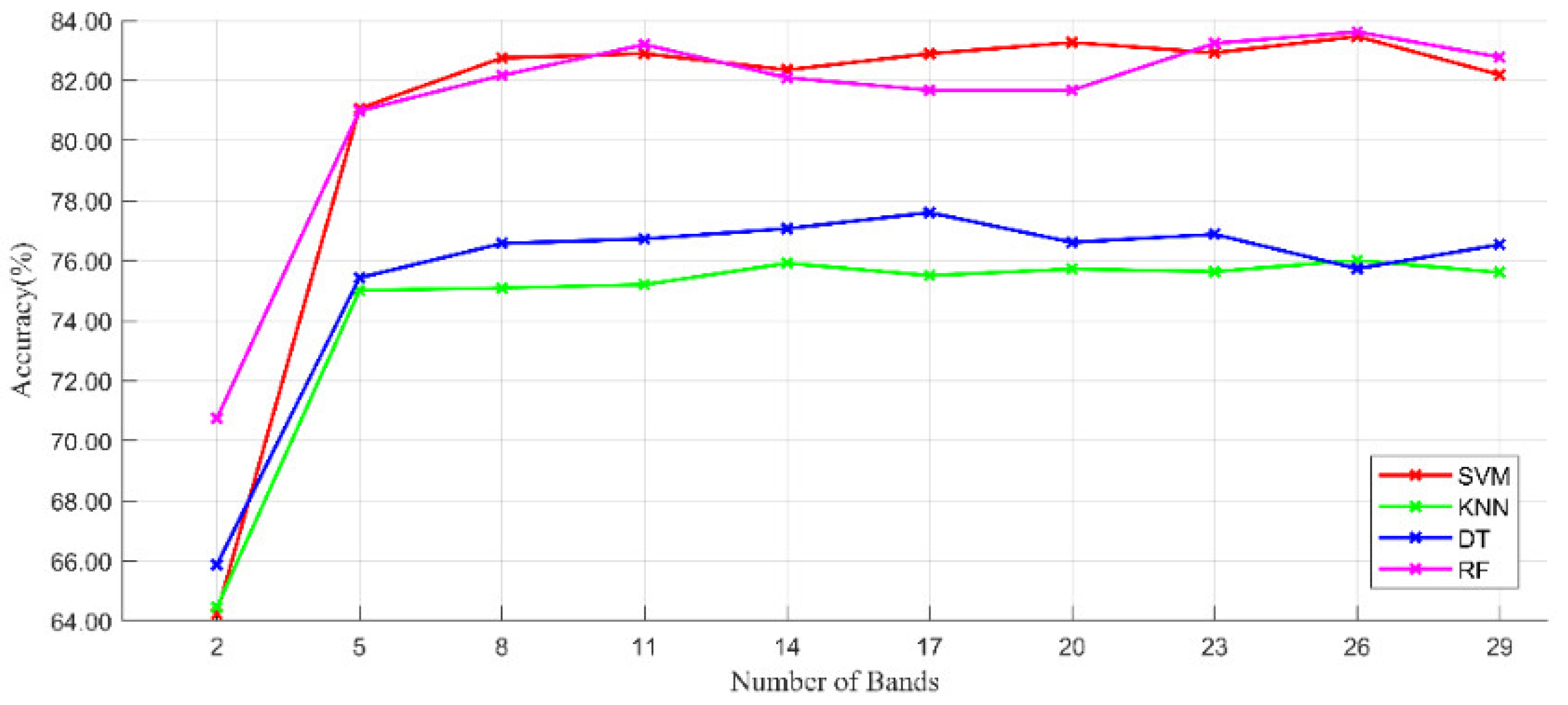Various strategies have been proposed to select a suitable subset of bands, such as ranking strategy, search strategy, sparse strategy, and clustering strategy [24]. In the unsupervised band selection method, the clustering-based approach aggregates all bands into different classes or subspaces and selects the bands closest to the center of the clusters. Xie et al. [25] used primarily the K-means algorithm to continuously calculate the distance between all sample points and the current candidate centers to determine the final clustering center, and then, by traversing all clusters, to select the feature bands. Qian et al. [26] proposed a sample-based affinity propagation clustering algorithm that considers the correlation between individual bands and obtained a subset of feature bands by maximizing the objective function. For LCC in heterogeneous mining areas, it is essential to select the effective band subset for HSI.

The method of joint spatial-spectral features utilizes both the spectral features of hyperspectral data and the spatial feature information of images. Kang et al. [27] used the SVM algorithm and spatial-spectral features to determine the probability of each pixel belonging to a different category. With the continuous advances of deep learning (DL) algorithms, more DL-based methods have been applied to HSI classification owing to their powerful deep feature capture capabilities [28,29,30,31,32,33,34]. Zheng et al. [35] studied a learning framework without patches to consider the global information of HSI. In addition, recurrent neural networks (RNN) [36], DBNs [37], and generative adversarial networks (GAN) [38] have also been frequently used for HSI classification. Chen et al. [39] used a joint channel-space attention mechanism and GAN (JAGAN) model and HSI to classify complex mining landscapes. However, CNNs are most widely used algorithms to capture deep features in HSI classification tasks. Hu et al. [40] used a one-dimensional CNN for HSI classification, and only used spectral information, while Zhong et al. [41] proposed a CNN model with a separate two-channel to obtain spectral and spatial features. Makantasis et al. [42] used a two-dimensional CNN (2D-CNN) that treat spectral bands as feature maps and encode the spectral and spatial information of pixels. Chen et al. [43] proposed a 3D-CNN model with an L2 regularization spectral and spatial feature extraction method in the classification of HSI. Roy et al. [33] used 2D-CNN to learn high-level features and 3D-CNN to learn low-level features, which improved classification performance with fewer parameters.

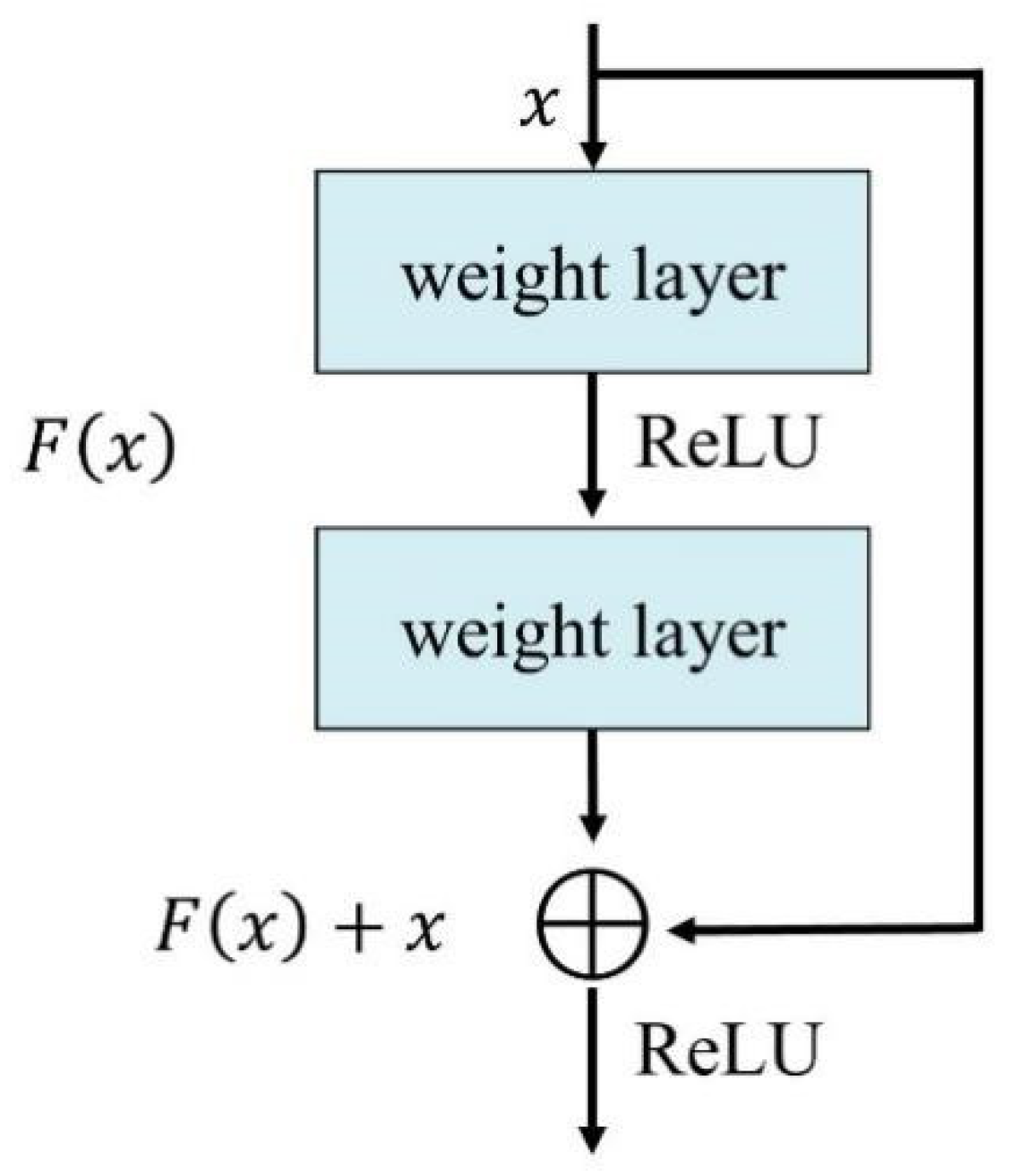
However, traditional CNNs are limited by gradient vanish as the network depth increases, the weights between the layers closer to the input layer cannot be effectively corrected due to how the derivative tends to 0, which may ultimately reduce the classification performance. The gradient often becomes extremely small during the conduction to the input layer, which then causes the connection weights in the lower layers to virtually cease to be updated, and the training never converges to an optimal solution [44]; to overcome this, residual networks (ResNet) have been proposed [45]. The internal residual block adds the block’s input directly to the block’s output and activates the ReLU function. A ResNet is constructed by considering several of these residual blocks.

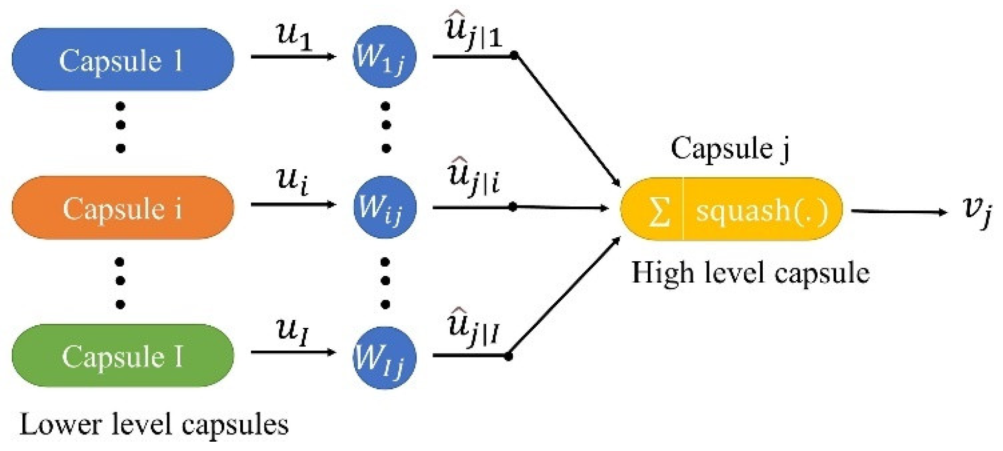
Furthermore, CNNs usually use scalars to represent information, and the ability to exploit the relationships between features detected at different locations in an image is rather limited. When the spatial location of feature information changes, it is difficult for CNNs to identify features. To extract more information, it is necessary to continuously deepen the network layer. The capsule network (CapsNet) [46] uses capsule vectors and dynamic routing to represent features, which can effectively reveal and learn the discriminative features, and expands new ideas for image classification. Unlike traditional CNN models, these vectors in CapsNet can store the orientation of features. As a result, CapsNet can accurately identify even when the position or angle of the same object changes. Importantly, land covers in heterogeneous mining areas have spatial autocorrelation [47], and the spatial pattern of remote sensing features may be captured by CapsNet.

Recently, CapsNet has been used in hyperspectral remote sensing image applications. Wang et al. [48] designed the CapsNet-TripleGAN framework to generate samples and classify HSI efficiently, while Zhu et al. [49] used a new CapsNet named Conv-CapsNet, reducing the number of model parameters and alleviating the overfitting issue in classification. Paoletti et al. [50] designed a spectral and spatial CapsNet, which can achieve high-precision classification results of his, while Li et al. [51] developed a robust CapsNet-based two-channel framework to fuse hyperspectral data with light detection and ranging-derived elevation data for classification. To learn higher level features, Yin et al. [52] proposed a new architecture to initialize the parameters of the CapsNet for better HSI classification.

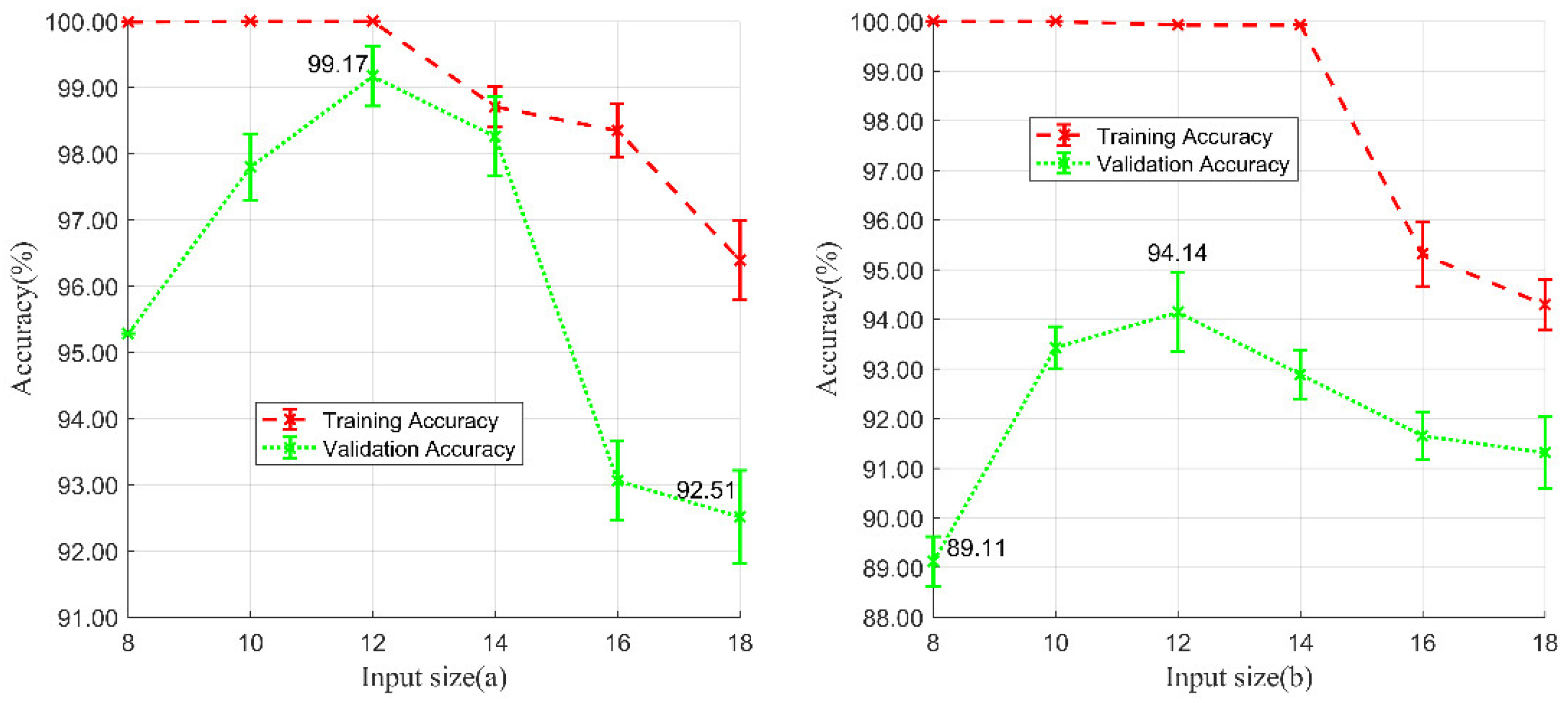
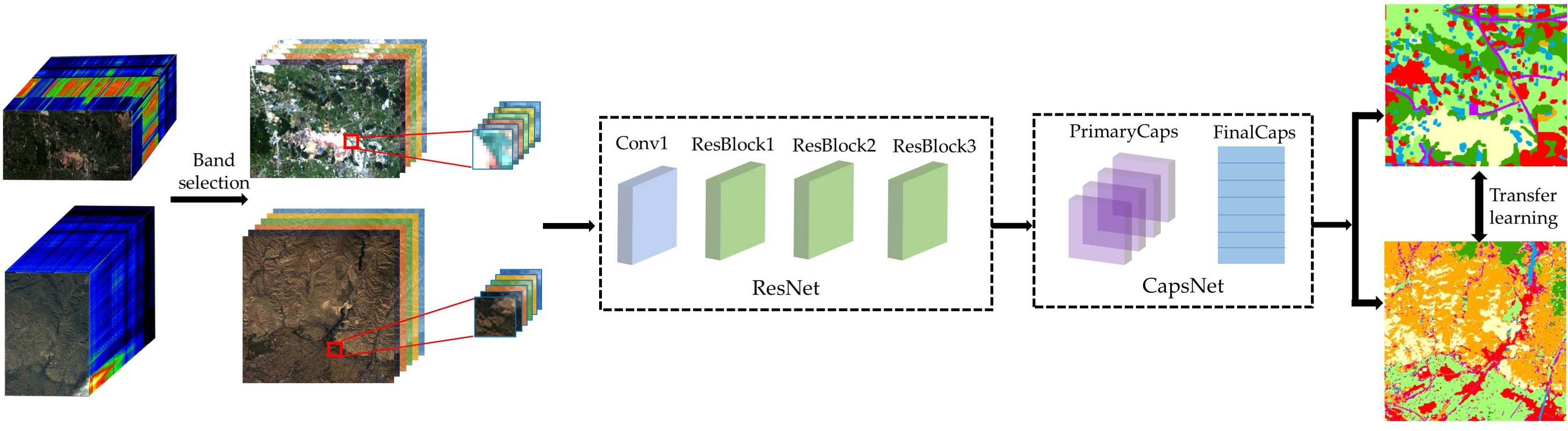
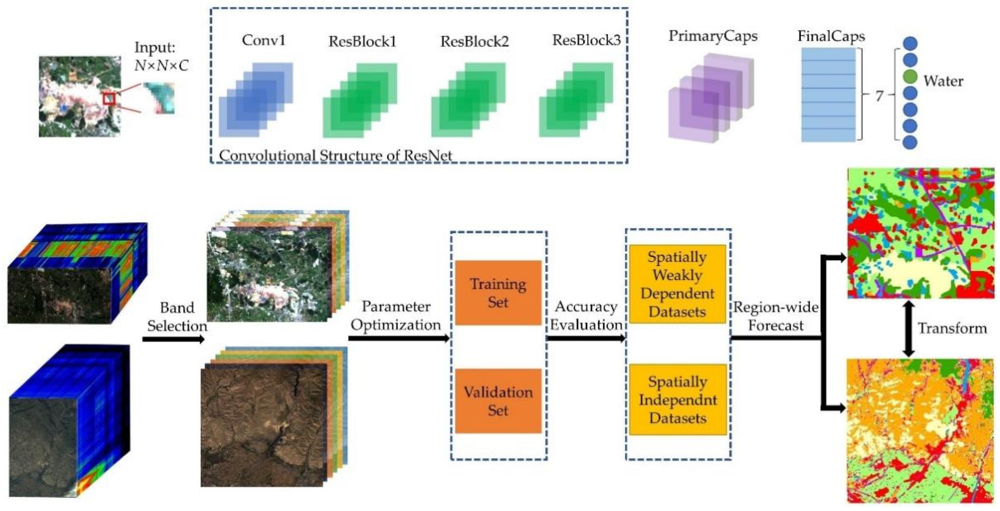
To extract useful spatial and spectral features from HSI, a combined model of ResNet and CapsNet (ResCapsNet) was proposed and tested with Gaofen-5 (GF-5) imagery in this study. There were three main contributions as follows:

(1) A novel framework of ResCapsNet for LCC in heterogeneous mining areas was proposed. First, a clustering-based semi-automated band selection method was conducted to determine the input bands. The ResNet was then used for extraction of deep HSI features, and the high-level features were put into a CapsNet for classification.

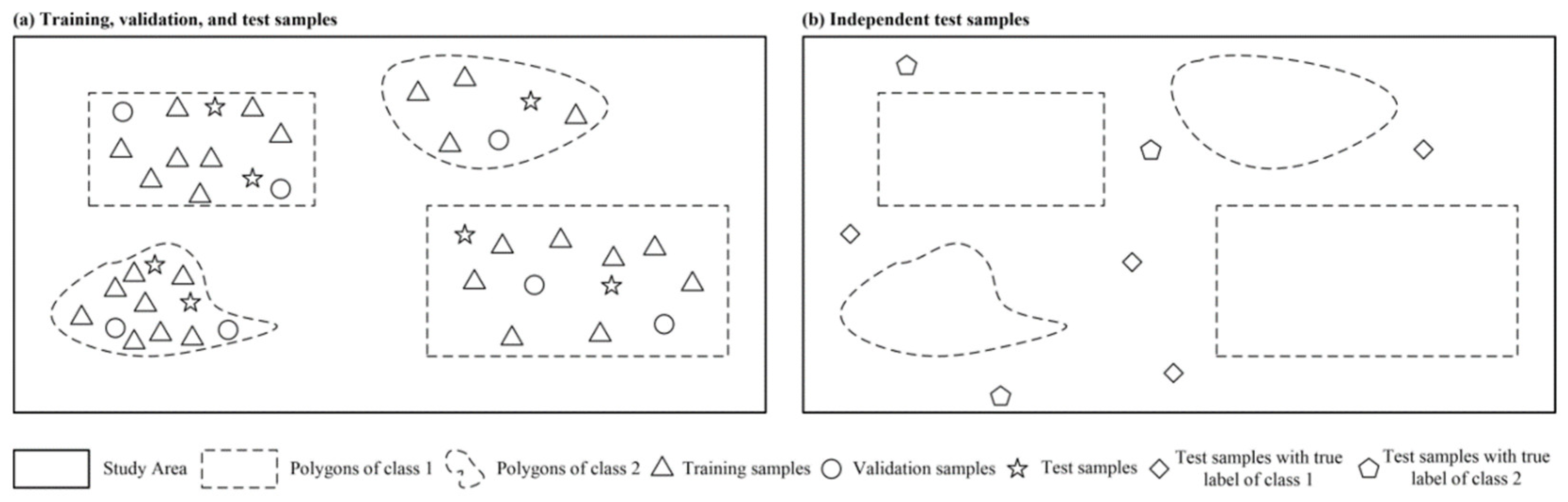
(2) The model was tested on two datasets (a spatially weakly dependent dataset and a spatially basically independent dataset) of two different areas captured by the GF-5 satellite. The purpose of designing two datasets is to test the spatial autocorrelation [47] of land cover areas in the experimental area.

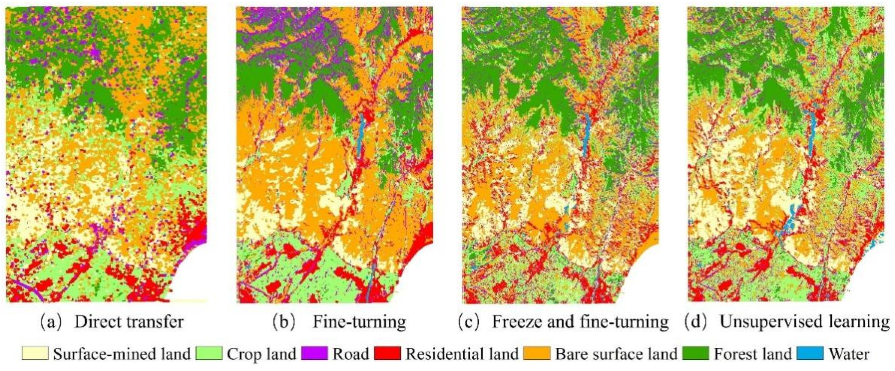
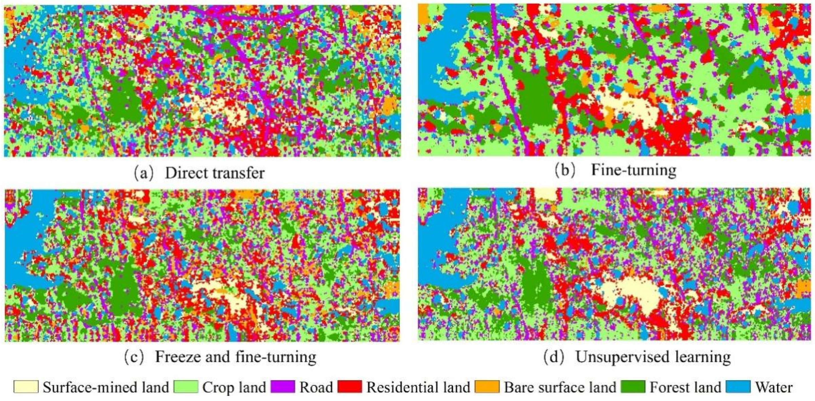
(3) Four transfer learning methods were investigated for cross-training and prediction of those two areas, i.e., direct transfer of trained models for prediction of other areas (hereafter referred to as direct transfer), fine-tuning of trained models (hereafter referred to as fine-tuning), freeze of part structure and fine-tuning (hereafter referred to as free and fine-tuning), and unsupervised feature learning based on maximum mean discrepancy (MMD) [53] (hereafter referred to as unsupervised learning).

2. Study Areas and Remote Sensing Data Source

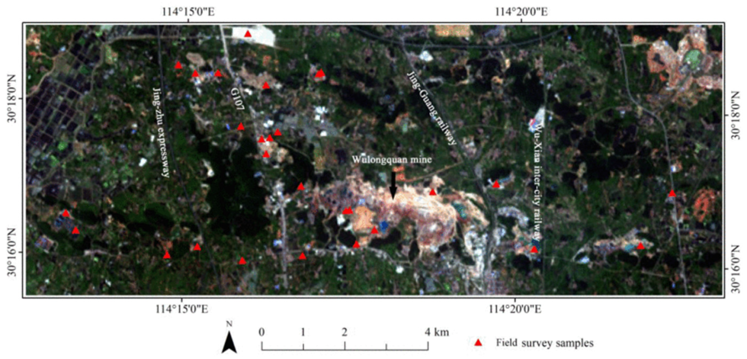
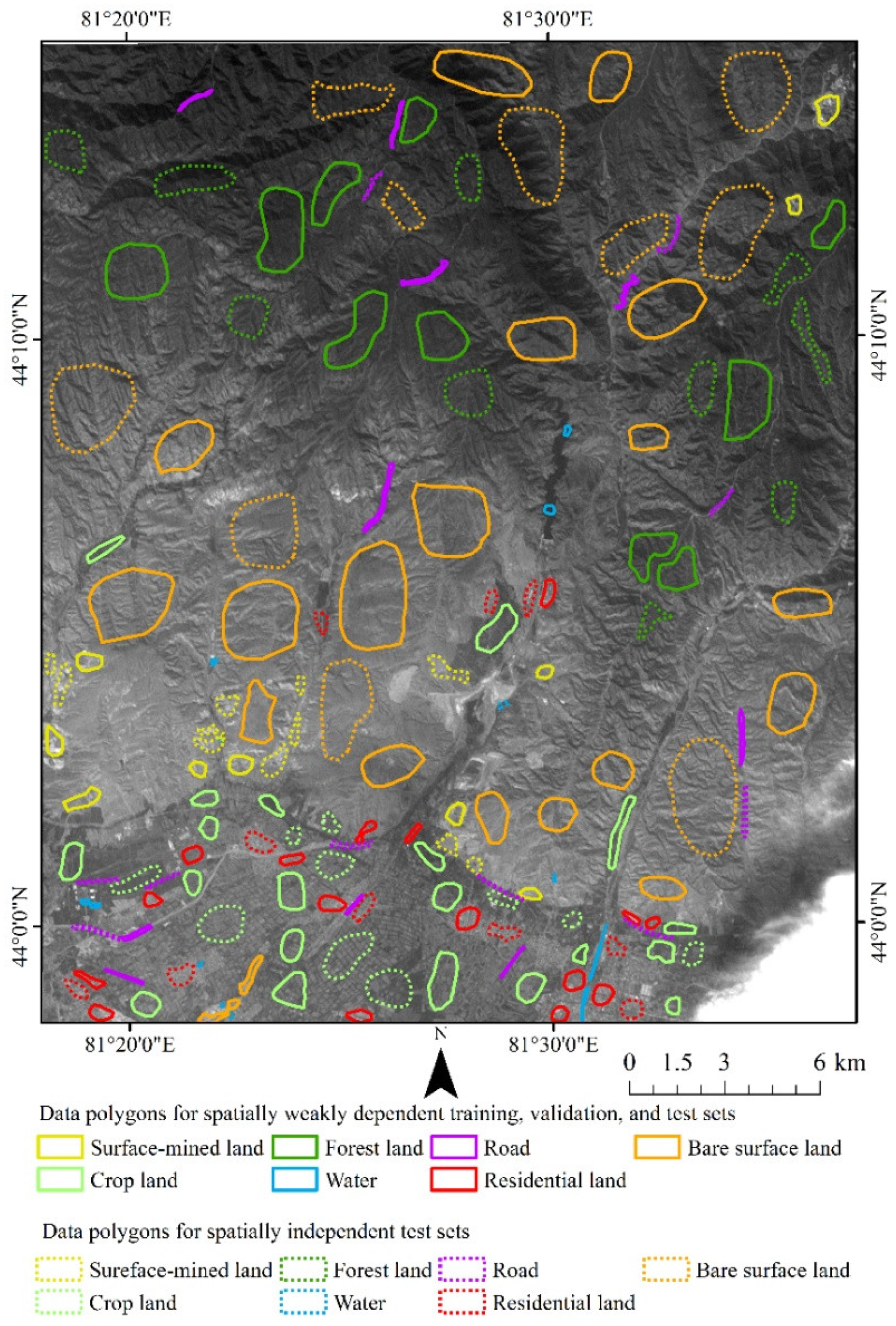
We selected an area in the Jiangxia District of Wuhan City, China (hereafter referred as to Wuhan study area) [10,54] (Figure 1), which belongs to the northern subtropical monsoon and humid climate zone characterized by hot summers and cold winters, abundant sunshine, four distinct seasons, and sufficient rainfall. This area also contains some surface mining and agricultural activities.

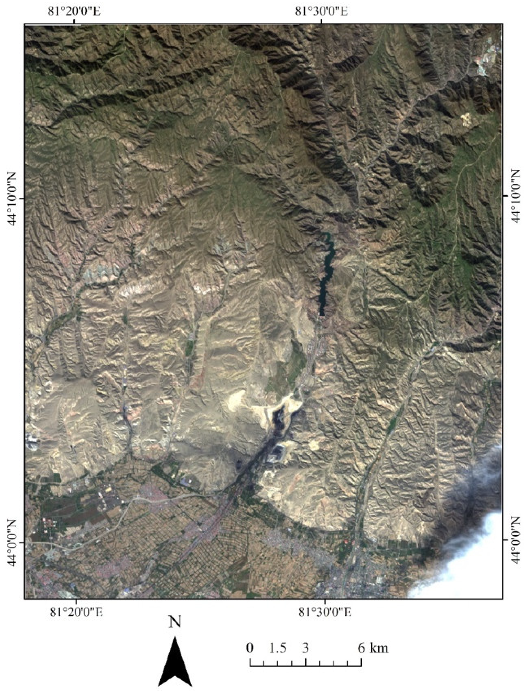
Another study area located in the Ili Kazakh Autonomous Prefecture of Xinjiang Province, China (hereafter referred as to Xinjiang study area) (Figure 2) characterized by mountains and vast inter-mountain plains, basins, and river valleys, and has a typical temperate continental arid climate was also selected. The average natural precipitation is 155 mm. There are also some surface mining activities.

The GF-5 images on 9 May 2018 and 25 September 2019 for the two areas were obtained. Radiometrically calibrated and orthorectification correction were conducted [39]. The GF-5 satellite, successfully launched in May 2018, can conduct comprehensive observations of the land and atmosphere at the same time, and can obtain the spectrum range from visible and near-infrared (VNIR) to shortwave infrared (SWIR) (i.e., from 400 to 2500 nm) with a width of 60 km and a spatial resolution of 30 m. There are 330 spectral channels. The GF-5 has two different spectral resolutions: 5 nm for VNIR and 10 nm for SWIR.

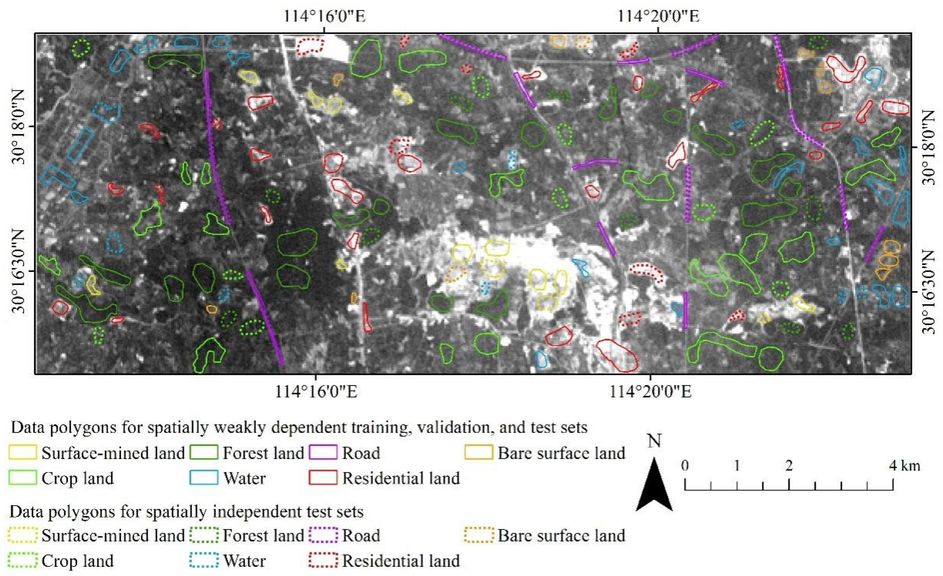
According to the requirements of mine environmental monitoring in China and the previous study [10], the LCC types were divided into seven categories namely road, cropland, water, residential land, forest land, bare land, and surface-mined land. Details are shown in

Table 1. Land cover classification scheme in the study.

No.	Class Name	Description
1	Surface-mined land	Mining operation area including mine buildings, waste rock piles, and mining fields.
2	Cropland	Crops with vegetation coverage mixed with bushes, including paddy fields and small amount fallow land
3	Forest land	Areas with a lot of forests., including woodland, nurseries, orchard, and shrubs.
4	Water	Areas containing water, including lakes, ponds and mining sumps.
5	Road	Roads are presented in strips with unique topological properties, including cement and asphalt roads.
6	Residential land	Commercial, industrial, and civil construction land, including urban land and rural residential areas.
7	Bare surface land	Exposed land with little vegetation, including bare soil lands, beaches.

.

3. Methods

3.1. ResCapsNet Model

The framework of the ResCapsNet model is presented in Figure 3. The network structure consists of three parts: Band selection, ResNet for feature extraction and CapsNet for classification.

We used a cluster-based band selection method to reduce the number of input bands. We adopted the ResNet-34 structure and modified it to fit hyperspectral remote sensing image data. ResNet-34 consists of four parts, having three, four, six, and three residual blocks, respectively. There are 64, 128, 256, and 512 filters for each recognition block in each section, respectively. To adapt to the input of the subsequent CapsNet and improve the accuracy of the model, we deleted the last filters. In our experiment, because the input size is too small, we set the stride of the convolution layer in ResBlock2 and ResBlock3 to 1.

The size of the convolution kernel in PrimaryCaps was 3 × 3. As the datasets used contained seven classes, the number of output capsules in FinalCaps was set to 7.

3.1.1. Band Selection

Directly processing the rich spectral information contained in hyperspectral images requires enormous computational effort. Band selection is an effective and straightforward method used to reduce redundancy without affecting the original content. Band selection is to select a representative and unique set of bands from the original hyperspectral image. In this study, we used the optimal clustering framework [55] to obtain the basic band subsets. The basic idea of this clustering algorithm is to evaluate the contribution of each band combination individually and then sum these contributions as a measure of the result of the overall band combination. We then input the extracted band subsets into four machine learning methods (SVM, random forest, decision tree, and k-nearest-neighbor (KNN)) for image classification experiments. Subsequently, the determined band subset was combined with the four true-color and false-color bands of the image. Finally, we used a trial-and-error based ResCapsNet model to determine the optimal band subset.

3.1.2. The Basic Structure of Residual Network

To obtain more abundant and detailed features, the method of deepening the network structure is generally adopted. However, traditional CNNs suffer from performance degradation when the network layer is too deep. Using a ResNet model avoids the negative feedback effect while deepening the number of network layers. The implementation of this mechanism mainly relies on the unique residual learning module (Residual learning) of the ResNet model. Figure 4 shows a schematic diagram of the residual learning module.

From Figure 4, in the process of backpropagation of the deeper network model, the existence of the residual learning module can ensure the direct propagation of the gradient and prevent the vanish and explosion of the gradient. The mathematical expression of the residual learning module is expressed in Equations (1) and (2):

$$y_l=x_l+F\left(x_l,w_l\right)$$

(1)

$$x_{l+1}=f\left(y_l\right)$$

(2)

where $x_l$ and $x_{l+1}$ are the input feature data and output feature data of the $l$th residual learning unit, $F()$ is the transformation function of the residual learning unit, while $f()$ is the nonlinear activation function ReLU.

Therefore, the mathematical relationship between the feature $x_l$ from the bottom layer of the network model and the deep feature $x_L$ can be established as:

$$x_L=x_l+{\displaystyle \sum }_{i=l}^{L-1}F\left(x_i,w_i\right)$$

(3)

3.1.3. Basic Structure of CapsNet

CapsNet is a new network structure made up of capsules rather than neurons. CapsNet uses vectorized neurons instead of traditional scalar neurons, which are more robust to the affine transformation of classification targets and require fewer training samples. A capsule consists of several scalar neurons, whose orientation indicates its properties, while the length represents the existence probability of the specific object. CapsNet use this feature to learn part–whole relationships between different objects and can deal with the problem of traditional CNNs using fully connected layers, which are unable to effectively represent the hierarchical structure of each detail of the objects. Figure 5 illustrates the way that CapsNet routes the information from one layer to another layer by a dynamic routing mechanism [56]. The essence of dynamic routing is that the low-level capsule sends its output to the high-level capsule through voting, in which the consistency is measured by the dot product of the vector [56].

In addition to the basic input and output layers, CapsNet also consists of convolutional layers, a PrimaryCaps layer, and a FinalCaps layer. The convolutional layers are used to capture the low-level features of the ground object. The PrimaryCaps layer is used to express the spatial relationship between the features. The extracted features are passed to the FinalCaps layer. The dynamic routing algorithm is used for prediction. The objective function of CapsNet is defined as:

$$L_k=T_{k}max{\left(0,m^{+}-\Vert v_k\Vert \right)}^2+\lambda \left(1-T_k\right)max{\left(0,\Vert v_k\Vert -m^{-}\right)}^2$$

(4)

Here $T_k$ = 1 if the true class is $k$ and zero otherwise, $v_k$ represents the module length of the capsule vector, $m^{+}$ and $m^{-}$ are hyper-parameters that indicate enough confidence of the existence or inexistence of a certain category, and $\lambda$ is a coefficient to prevent the network from falling into the local optimal weight coefficient.

The dynamic routing algorithm adjusts the coupling coefficient $c$ according to the similarity between the capsules of the lower level and the capsules of higher level and updates the weights $W$ between the networks accordingly. If the similarity between low-level capsule $i$ and the high-level capsule $j$ is greater, the coupling coefficient $c_{ij}$ is also greater. The specific calculation formula is:

$$c_{ij}=\frac{\exp \left(b_{ij}\right)}{{{\displaystyle \sum }}_k\exp \left(b_{ij}\right)}$$

(5)

where $b_{ij}$ is the log probability of whether capsule $i$ should be coupled with capsule $j$ and is set to 0 initially. The update mode is:

$$b_{ij}\leftarrow b_{ij}+{\widehat{u}}_{j\mid i}{v}_j$$

(6)

Among these, ${\widehat{u}}_{j\mid i}$ is obtained from capsule $u_i$ through affinity transformation, and its calculation method is shown in Equation (7). $v_j$ represents the output vector of capsule $j$, and to make sure that the length of $v_j$ is between 0 and 1, the activation function is Squash instead of ReLu. The activation function Squash is:

$${\widehat{u}}_{j\mid i}=W_{ij}{u}_i$$

(7)

$$v_j=\frac{{\Vert s_j\Vert }^2}{1+{\Vert s_j\Vert }^2}\frac{s_j}{\Vert s_j\Vert }$$

(8)

where $s_j$ represents the output vector of capsule $j$, and can be calculated as follows:

$$s_j={\displaystyle \sum }_i{c}_{ij}{\widehat{u}}_{j\mid i}$$

(9)

3.2. Training, Validation, and Test Sets

As shown in Figure 6a, we select training, validation, and test points from the data polygons at the same time. The points are independent and located in the same data polygons with small areas. Therefore, we refer to them as spatially weakly dependent datasets. As shown in Figure 6b, we additionally select test samples outside the former data polygons, which are spatially distant from the training data polygons. Therefore, we refer to these as spatially independent datasets.

3.2.1. Spatially Weakly Dependent Datasets

We use two spatially weakly dependent datasets to initially evaluate the accuracy of the model. For each of the seven land cover types in the study area, 200 sample points (pixels) were selected as the training sets, 100 sample points (pixels) as the validation sets, and 200 sample points (pixels) as the test sets. These samples are obtained by stratified random sampling from within these solid digital polygons, independent of each other.

Figure 7 and Figure 8 show the distribution of the data polygons over the study area, which were used to randomly select the sample points. The training sets were used for model training. Validation sets were mainly used to select and optimize parameters. The test sets were used for accuracy assessment. The percentages and associated data polygons for each set in the two study areas are listed in

Table 2. Sampling description of spatially weakly dependent datasets in the Wuhan study area.

Types	Number of DPs	Area of DPs	Ratio 1	Ratio 2
Surface-mined land	10	0.63	10.23	1.13
Cropland	20	3.53	9.52	0.24
Forest land	20	3.25	10.82	0.21
Water	20	1.36	9.86	0.1
Road	10	0.36	10.29	1.13
Residential land	25	1.71	10.15	0.19
Bare surface land	7	0.26	13.20	1.13

Number and area (km²) of data polygons (DPs). Ratio 1: ratio (%) of the area occupied by training, validation, and test sets to the total area. Ratio 2: ratio (%) of the area occupied by the training pixels to the total area.

and

Table 3. Sampling description of spatially weakly dependent datasets in the Xinjiang study area.

Types	Number of DPs	Area of DPs	Ratio 1	Ratio 2
Surface-mined land	10	2.82	9.86	1.57
Cropland	20	9.78	9.97	0.46
Forest land	10	17.81	10.47	0.26
Water	8	0.27	12.23	20.20
Road	10	1.04	10.57	4.59
Residential land	16	3.35	10.00	1.34
Bare surface land	20	43.52	9.97	0.10

Number and area (km²) of data polygons (DPs). Ratio 1: ratio (%) of the area occupied by training, validation, and test sets to the total area. Ratio 2: ratio (%) of the area occupied by the training pixels to the total area.

.

3.2.2. Spatially Independent Datasets

The accuracy and robustness of the model were further evaluated using two spatially basically independent datasets, where the data polygons were spatially independent from those data polygons selected by spatially weakly dependent datasets. We selected 200 sample points (pixels) as the training sets, 100 sample points (pixels) as the validation sets and 200 sample points (pixels) as test sets. The training and validation samples come from solid data polygons in the weakly dependent dataset, but the test samples come from dashed data polygons that are spatially independent. The percentages and associated data polygons for each set in the two study areas are listed in

Table 4. Sampling description of spatially independent datasets in the Wuhan study area.

Types	Number of DPs	Area of DPs	Ratio 1	Ratio 2
Surface-mined land	4	0.24	3.84	0.45
Cropland	10	0.73	1.95	0.24
Forest land	10	0.54	1.79	0.21
Water	20	0.38	2.74	0.10
Road	10	0.48	13.56	1.13
Residential land	25	0.48	2.71	0.19
Bare surface land	7	0.18	9.17	0.56

Number and area (km²) of data polygons (DPs). Ratio 1: ratio (%) of the area occupied by training, validation, and test sets to the total area. Ratio 2: ratio (%) of the area occupied by the training pixels to the total area.

and

Table 5. Sampling description of spatially independent datasets in the Xinjiang study area.

Types	Number of DPs	Area of DPs	Ratio 1	Ratio 2
Surface-mined land	10	2.76	9.65	0.31
Cropland	10	6.30	6.42	0.09
Forest land	10	10.69	6.28	0.05
Water	6	0.11	5.01	4.04
Road	10	1.03	10.54	0.92
Residential land	10	2.71	8.08	0.2
Bare surface land	10	37.54	8.60	0.02

Number and area (km²) of data polygons (DPs). Ratio 1: ratio (%) of the area occupied by training, validation, and test sets to the total area. Ratio 2: ratio (%) of the area occupied by the training pixels to the total area.

. Figure 7 and Figure 8 show the distribution of the data polygons over the study area.

3.3. Parameter Optimization and Model Construction

In this study, input band, input size, batch size, and the number of dynamic routings were selected for model optimization, where the number of dynamic routes refers to the number of iterations of the dynamic routing algorithm. Five random experiments were conducted for each parameter optimization. Those parameter values with highest averaged validation accuracies were the results of parameter optimization. To simplify the parameter selection procedure, a trial-and-error method and various empirical values were used to set other parameters.

After parameter optimization, ResCapsNet and a combination of Res2Net [58] and CapsNet (hereafter referred to as Res2CapsNet) were constructed.

Four transfer learning methods were investigated for cross-training and prediction of those two areas, i.e., direct transfer, fine-tuning, freeze and fine-tuning, and unsupervised learning. Finally, the test accuracies and predicted maps were assessed.

3.4. Accuracy Evaluation Criteria

The training and validation sets were used for model training and parameter selection, while the test sets were used to conduct the quantitative evaluation. The averaged overall accuracy (OA), F1-score, and kappa coefficient (Kappa) were computed to evaluate the overall performances of the experimental results. In addition, we used the F1-measure of each class to further evaluate the proposed models. F1-score is the average value of all the F1-measures. F1-measure is a special case of F-score. F-measure is an index used to measure the accuracy of binary classification model in statistics. It considers both the precision and recall of the classification model. F-measure can be calculated by the following equation:

$$\mathrm{F}-\mathrm{measure}=\frac{a^2+1}{a^2}\ast \frac{precision\ast recall}{precision+recall}$$

(10)

where $a$ is the weight. When the weight a is equal to 1, the F1 score is obtained as follows:

$$\mathrm{F}1-\mathrm{measure}=\frac{2\ast precision\ast recall}{precision+recall}$$

(11)

These four criteria are valuable measures that show the performance of the classifications.

4. Results

4.1. Parameter Selection Results

4.1.1. Band Selection

Figure 9 shows that when more than eight bands (band set 1) are selected, the classification effect of the model begins to converge. However, these eight bands did not fully cover the blue, green, and red near-infrared bands of the hyperspectral images. The experiments in the discussion section in the literature [14] tested three models with different band combinations. This experiment demonstrated that using both true color and false color images as inputs was effective. To make better use of spectral information, we added the four true-color and false-color bands (20, 38, 59, 90) containing information on band set 1 and forming band set 2. Finally, we conducted multiple sets of experiments on the respapsnet model using a trial-and-error method. With high accuracy, we eliminated similar bands that possessed little information and obtained the final six bands as set 3. The parameters of input size, batch size, and number of dynamic routes were set to 12, 50, and 3 respectively, obtained by a simple trail-and-error method. From

Table 6. Validation accuracy of different band sets under the ResCapsNet model.

Band Set	Bands	Validation Accuracy
1	22, 46, 59, 66, 90, 107, 118, 270	97.42 ± 0.86%
2	20, 22, 38, 46, 59, 66, 90, 107, 118, 270	97.57 ± 0.41%
3	20, 59, 38, 90, 118, 270	98.53 ± 0.52%

, when the input bands are based on band sets 1 and 2, the validation accuracies of the model are 97.42 ± 0.86% and 97.57 ± 0.41%, respectively. Meanwhile, when the input bands are based on band set 3, the validation accuracy of the model is 98.53 ± 0.52%. Combined with the experimental efficiency and classification results, we selected band set 3 with six bands for subsequent experiments.

4.1.2. Input Size Selection

For this experiment, the input size started at 8 and increased to 18 in an interval of 2 (Figure 10). Each value of patch was applied to five random tests. Validation accuracies were at the maximum values (99.17 ± 0.46% and 94.14 ± 0.71%) for the input size of 12.

4.1.3. Batch Size Selection

For this experiment, we changed the size of the batch to select the most suitable parameters. Each experimental result is the average of five replicate experiments. As shown in Figure 11, when the batch size of 100 was applied, the networks achieved the highest validation accuracy (99.14 ± 0.52%) in the Wuhan study area, with a 1.10% improvement relative to the worst accuracy. When the batch size of 75 was applied, the networks achieved the highest validation accuracy (95.40 ± 0.58%) in the Xinjiang study area, with a 2.80% improvement relative to the worst accuracy.

4.1.4. Dynamic Routing Number Selection

The routing number is an important parameter in the dynamic routing algorithm, the essence of which is that the lower-level capsules send their output to the higher-level consistent capsules by voting [56]. Selecting a suitable routing number can make the proposed models obtain the best coupling coefficient. Thus, a series of routing numbers ranging from 3 to 21, in intervals of 3, were applied in this experiment. As shown in Figure 12, when the iteration number was set to 15, the model achieved optimal results on validation accuracies. Smaller values can lead to insufficient training, while larger values will lead to a lack of optimal fit and increase the training time. Considering this, we selected 15 as the number of routes in the subsequent experiments.

4.2. Accuracy Evaluation Result

4.2.1. Overall Performance

After the parameter adjustment step, the optimal model was obtained.

Table 7. Overall performance of different models on spatially weakly dependent datasets in the Wuhan study area.

Model	OA (%)	F1-Score (%)	Kappa (%)
SVM	82.73 ± 0.37	82.54 ± 0.43	79.56 ± 0.45
RF	82.58 ± 0.21	82.44 ± 0.27	79.51 ± 0.38
CapsNet	85.52 ± 0.67	85.31 ± 0.64	82.78 ± 0.67
ResNet	97.62 ± 0.31	97.59 ± 0.37	97.18 ± 0.32
CNN	94.14 ± 0.28	93.78 ± 0.59	93.69 ± 0.38
Res2CapsNet	96.01 ± 0.42	96.05 ± 0.35	95.35 ± 0.42
ResCapsNet	98.45 ± 0.23	98.43 ± 0.21	98.15 ± 0.30

SVM, support vector machine; RF, random forest; Resnet, deep residual network; CapsNet, capsule network; CNN, convolutional neural network (Visual Geometry Group Network16); Res2CapsNet, combination of Res2Net and CapsNet; ResCapsNet, combination of ResNet and CapsNet.

,

Table 8. Overall performance of different models on spatially independent datasets in the Wuhan study area.

Model	OA (%)	F1-Score (%)	Kappa (%)
SVM	79.94 ± 0.23	78.67 ± 0.26	79.56 ± 0.32
RF	73.84 ± 0.64	71.71 ± 0.47	70.26 ± 0.56
CapsNet	72.19 ± 0.46	70.11 ± 0.44	66.88 ± 0.46
ResNet	81.58 ± 0.33	80.30 ± 0.28	79.04 ± 0.31
CNN	80.33 ± 0.62	78.00 ± 0.58	75.32 ± 0.65
Res2CapsNet	80.44 ± 0.84	78.68 ± 0.92	77.05 ± 0.81
ResCapsNet	82.80 ± 0.25	81.34 ± 0.27	79.69 ± 0.24

SVM, support vector machine; RF, random forest; Resnet, deep residual network; CapsNet, capsule network; CNN, convolutional neural network (Visual Geometry Group Network16); Res2CapsNet, combination of Res2Net and CapsNet; ResCapsNet, combination of ResNet and CapsNet.

,

Table 9. Overall performance of different models on spatially weakly dependent datasets in the Xinjiang study area.

Model	OA (%)	F1-Score (%)	Kappa (%)
SVM	73.88 ± 0.26	73.03 ± 0.26	69.52 ± 0.30
RF	71.80 ± 0.57	71.72 ± 0.49	67.41 ± 0.54
CapsNet	86.34 ± 0.55	86.63 ± 0.58	84.61 ± 0.55
ResNet	92.03 ± 0.49	92.96 ± 0.53	91.32 ± 0.48
CNN	87.63 ± 0.57	86.47 ± 0.54	85.42 ± 0.71
Res2CapsNet	89.05 ± 0.13	88.86 ± 0.13	87.14 ± 0.14
ResCapsNet	92.82 ± 0.28	92.74 ± 0.24	91.60 ± 0.29

SVM, support vector machine; RF, random forest; Resnet, deep residual network; CapsNet, capsule network; CNN, convolutional neural network (Visual Geometry Group Network16); Res2CapsNet, combination of Res2Net and CapsNet; ResCapsNet, combination of ResNet and CapsNet.

and

Table 10. Overall performance of different models on spatially independent datasets in the Xinjiang study area.

Model	OA (%)	F1-Score (%)	Kappa (%)
SVM	63.43 ± 0.39	61.73 ± 0.43	57.47 ± 0.36
RF	59.43 ± 0.82	56.99 ± 0.78	50.58 ± 0.83
CapsNet	64.91 ± 0.67	62.09 ± 0.71	56.83 ± 0.66
ResNet	68.93 ± 0.54	63.24 ± 0.58	59.93 ± 0.56
CNN	65.58 ± 0.84	65.01 ± 0.63	59.85 ± 0.86
Res2CapsNet	66.69 ± 0.12	62.28 ± 0.11	58.23 ± 0.17
ResCapsNet	70.88 ± 0.39	65.22 ± 0.35	62.32 ± 0.39

SVM, support vector machine; RF, random forest; Resnet, deep residual network; CapsNet, capsule network; CNN, convolutional neural network (Visual Geometry Group Network16); Res2CapsNet, combination of Res2Net and CapsNet; ResCapsNet, combination of ResNet and CapsNet.

present the overall performances of the four datasets using different models, considering the OA, F1-score, Kappa as indicators.

In comparison, the SVM and RF algorithms showed the worst performance, while the rest of the DL-based algorithms performed significantly better. ResCapNet achieved the best OA, with 98.45 ± 0.23% and 82.80 ± 0.25% for the datasets in Wuhan. The best OA of the spatially weakly dependent datasets in Wuhan was 19.00%, 19.22%, 15.12%, 0.85%, 4.58%, 2.54% higher than those for SVM, RF, CapsNet, ResNet, CNN, and Res2NetCapsNet, respectively. The best OA of the spatially independent datasets in Wuhan increased 3.58%, 12.13%, 14.70%, 1.50%, 3.07%, and 2.93% compared with SVM, RF, CapsNet, ResNet, CNN, and Res2NetCapsNet, respectively.

The DL based methods mostly outperform the machine learning methods on both datasets. The results also illustrate the superiority of DL-based methods, hence the wide usage of DL algorithms in HSI classification. Compared with other methods, our model performs better on these metrics. For the spatially weakly dependent and independent datasets, the ResCapsNet achieves a test accuracy of 92.82% ± 0.28% and 70.88% ± 0.39%.

The best OA of the spatially weakly dependent datasets in Xinjiang is 25.64%, 29.28%, 7.51%, 0.86%, 5.92% and 4.01% higher than those of SVM, RF, CapsNet, ResNet, CNN, and Res2NetCapsNet, respectively. The best OA of the spatially independent datasets in Xinjiang increased by 11.75%, 19.27%, 9.20%, 2.83%, 8.08%, and 6.28% compared with SVM, RF, CapsNet, ResNet, CNN, and Res2NetCapsNet, respectively.

4.2.2. Class-Specific Performance

Tables S1–S4 quantitatively represent the individual class accuracies obtained by different methods for the various datasets in the two study areas.

In the weakly dependent datasets in Wuhan, ResCapsNet provided the highest F1-measure values for surface-mined land (99.27%), cropland (98.44%), forest land (95.71%), water (99.32%), residential land (97.69%), and bare surface land (100%). ResNet provided the highest values for roads (99.53%). In the spatially independent datasets in Wuhan, ResCapsNet provided the highest F1-measure values for forest land (100%), residential land (85.24%) and bare surface land (76.44%). ResNet provided the highest values for surface-mined land (79.04%) and cropland (93.25%). SVM provided the highest value for roads (81.02%). Moreover, both methods based on machine learning performed better in the classification of roads.

In the weakly dependent datasets in Xinjiang, ResCapsNet provided the highest F1-measure values for cropland (95.91%), forest land (97.86%), water (98.98%), residential land (96.84%), and bare surface land (79.76%); ResNet provided the highest values for surface-mined land (93.69%) and roads (92.75%). In the spatially independent datasets in Xinjiang, ResCapsNet provided the highest F1-measure values for cropland (85.29%), forest land (96.27%), roads (28.85%), and residential land (90.13%); ResNet provided the highest value for bare surface land (66.27%), and SVM provided the highest value for surface-mined land (82.24%). RF and CapsNet outperformed the other models in the classification of water. In the spatially independent dataset, the overall classification accuracy of roads was low, which may be due to the large difference between roads in mountainous areas and urban and rural roads.

4.2.3. Assessment of Predicted Maps

To qualitatively evaluate the results, classification maps based on each well-trained model are illustrated in Figure 13 and Figure 14. Compared with those derived from the other models, ResCapsNet achieved better results. The ResCapsNet classification map has less noise and a lower rate of misclassification. From the visualization results, using CapsNet alone had a better effect on land classification with low spatial complexity, since it is more sensitive to spatial features. When ResNet was used alone, the land classification results with high spatial complexity were better. Their combination reduced the impact of spatial complexity on the classification results. As such, we achieved relatively robust representations compared with the two models.

From Figure 13, one can see that our model has better land cover classification accuracy in the Wuhan study area. For example, in the yellow box in the upper left corner of Figure 13g, our model better distinguished forest land from roads compared with the CNN. Within the black box, our model was obviously better than the other models in classifying the mining land, and could also identify the water body in the mining land and surrounding residential land well. Within the blue oval area, our model had less salt and pepper noise in the classification of cultivated land, while the other models had obvious errors (e.g., misclassification as roads).

From the overall classification of the Xinjiang research area (Figure 14), the method based on DL was better than that based on machine learning. DL could identify the image information in a patch and make better use of the spatial information. ResCapsNet was better than the other models in several areas. For example, in the black area in Figure 14g, our model could better identify woodland and bare land, and the error rate was lower than that of the other models. Within the blue box, the other models had omission errors in the classification of bare land and roads. Although some roads were misclassified as residential or bare surface land, the overall shape and length of the roads could be easily discerned. The main factors lie in the following aspects: (1) The samples randomly selected for training, validation, and testing did not have complete independence, which may have caused the samples to be less representative, and (2) Owing to the resolution of the GF-5 satellite, the width values of some roads were less than 1 pixel and could be easily divided into neighboring types.

4.3. Model Transfer between the Two Study Areas

We conducted four sets of experiments to compare the results of different methods for model transfer in two study areas, i.e., Wuhan and Xinjiang.

For direct transfer, after the model was trained on the dataset in the source study area, we directly predicted the test sets and the target study area. For fine-tuning, we used a small amount of data from the target study area (50 samples for each class) to train the model from the source study area. Then we used the trained model for prediction of the target area. For freeze and fine-tuning, we froze the ResNet part of the model that trained on the source study area, and then used the target study area data (50 samples for each class) to fine-tune the CapsNet. For unsupervised learning, we used the MMD to train the model, and then predicted the target area.

Table 11. Results of transforming from the Xinjiang study area to the Wuhan study area using different methods on spatially weakly dependent datasets.

Method	OA (%)	F1-Score (%)	Kappa (%)
Direct transfer	32.14	30.97	28.90
Fine-turning	96.29	96.30	95.67
Freeze and fine-tuning	83.93	83.80	81.10
Unsupervised learning	73.35	71.32	67.71

and

Table 12. Results of transforming from the Xinjiang study area to the Wuhan study area using different methods on spatially independent datasets.

Method	OA (%)	F1-Score (%)	Kappa (%)
Direct transfer	26.99	25.21	14.77
Fine-tuning	67.34	61.79	56.85
Freeze and fine-tuning	53.10	50.17	44.39
Unsupervised learning	61.68	58.31	55.72

present the results, while Figure 15 shows the predicted image of model transfer from the Xinjiang study area to the Wuhan study area though different methods. Results show that the fine-turning method achieves the highest precision in the testing of samples and prediction map.

Table 13. Results of transforming from the Wuhan study area to the Xinjiang study area using different methods on spatially weakly dependent datasets.

Method	OA (%)	F1-Score (%)	Kappa (%)
Direct transfer	33.16	26.36	24.63
Fine-tuning	93.18	93.14	92.04
Freeze and fine-tuning	78.22	77.84	74.23
Unsupervised learning	59.48	53.30	48.66

and

Table 14. Results of transforming from the Wuhan study area to the Xinjiang study area using different methods on spatially independent datasets.

Method	OA (%)	F1-Score (%)	Kappa (%)
Direct transfer	27.49	24.01	19.81
Fine-tuning	71.19	72.07	66.39
Freeze and fine-tuning	57.96	56.26	55.49
Unsupervised learning	43.55	38.32	35.47

show the results of transforming from the Wuhan study area to the Xinjiang study area. Figure 16 shows the predicted image of model transfer from the Wuhan study area to the Xinjiang study area though different methods. Results show that the fine-tuning method performs the best in the transfer experiments, while the methods based on freeze also have good accuracy in the testing of samples, but do not perform as well as the fine-turning-based method in the prediction map.

5. Discussion

5.1. Performances of ResCapsNet with Limited Samples

To assess the effectiveness of ResCapsNet with limited samples, we took 20, 30, and 50 points from the dataset of 200 points in each category as training sets. The same test sets were used for accuracy assessment. Table S5 lists the results of various models under different limited samples in the Wuhan study area, while Table S6 lists the results of various models under different limited samples in the Xinjiang study area.

From the experimental results, with increasing training data, the accuracy of ResCapsNet improved fastest, indicating that ResCapsNet has a relatively high demand for training data. For a small amount of samples, machine learning-based methods also produced excellent results, with some being better than DL-based models. The effect of the CNN model was close to optimal in the case of 20 samples, but with the increase in training samples, the improvement of experimental accuracy was less than that of other models.

For limited samples (e.g., 50 training sample points), in the Wuhan experimental area, ResNet’s OA was 85.54% and the Kappa was 82.29%; for CapsNet, the OA was 86.18% and the Kappa was 85.04%, which was second only to ResCapsNet’s OA.

In the Xinjiang experimental area, also taking 50 samples as an example, compared with the CNN, ResCapsNet was 2.2%, 6.4%, and 5.4% higher in terms of OA, F1-score, and Kappa, respectively.

In summary, by combining ResNet and CapsNet, we effectively extracted key features under limited samples and improved the classification accuracy.

5.2. Effectiveness of Different Data Input Sizes

As shown in Figure 10, different sizes of input data led to different classification accuracies. We conducted multiple sets of experiments on this parameter with models using deep networks and showed that different models require different input data sizes. In the Wuhan research area, the best field size for CapsNet was 12, and that for ResNet, CNN, and ResCapsNet were 10, 18, and 12, respectively. At the same time, there were also differences in the optimal input size of different study areas. For example, the best input size of ResNet in the Wuhan research area was 10, and 18 in the Xinjiang.

The Xinjiang study area contains several bigger patches of forest land and unused bare land, more suitable for a larger input size. Therefore, according to the study area, we should adjust the input size of the model. Input size that is too small cannot fully utilize spatial information, while an excessively large input size contains too much interference information.

5.3. Comparisons of Different Methods

We compared results with those of the JAGAN model [39] applied to a GF-5 image of the Wuhan study area. The OA, F1-score, and Kappa values of JAGAN were 86.09%, 85.86%, 79.41%, respectively. Those accuracies were much lower than our model.

The training points used by JAGAN were with the same numbers as for our study. However, our selected data polygons only accounted for 10% of the total area, which was smaller than that of Chen et al. [39] who used more test samples.

Besides, we produced a spatially independent dataset in our experiments for Wuhan study area. The predicted maps of those two models are shown in Figure 17. The prediction results by the JAGAN framework is more refined, but there are some areas of salt and pepper noise. The prediction map by ResCapsNet is smoother. Moreover, the bare surface land was not classified by Chen et al. [39].

6. Conclusions

For better LCC results in heterogeneous mining areas, we proposed a ResCapsNet model based on GF-5 imagery. The model took advantages of the clustering-based semi-automated band selection method, ResNet, and CapsNet.

Spatially weakly dependent and independent datasets in the Wuhan and Xinjiang study areas were used to test the proposed model. Our proposed method provided the best results for both datasets. Four transfer learning methods were investigated for cross-training and prediction of those two areas and achieved good results. In summary, our proposed model has high robustness and generalizability.

In the future we will focus on leveraging various hyperspectral images at different areas, as well as larger datasets, and will attempt more experiments on publicly classical hyperspectral image datasets.

References

1. Liu, X.; He, J.; Yao, Y.; Zhang, J.; Liang, H.; Wang, H.; Hong, Y. Classifying urban land use by integrating remote sensing and social media data. Int. J. Geogr. Inf. Sci. 2017, 31, 1675–1696. [Google Scholar] [CrossRef]
2. Hong, D.; Yokoya, N.; Xia, G.S.; Chanussot, J.; Zhu, X.X. X-ModalNet: A semi-supervised deep cross-modal network for classification of remote sensing data. ISPRS J. Photogramm. Remote Sens. 2020, 167, 12–23. [Google Scholar] [CrossRef] [PubMed]
3. Liu, J.; Xiang, J.; Jin, Y.; Liu, R.; Yan, J.; Wang, L. Boost Precision Agriculture with Unmanned Aerial Vehicle Remote Sensing and Edge Intelligence: A Survey. Remote Sens. 2021, 13, 4387. [Google Scholar] [CrossRef]
4. Chen, W.; Ouyang, S.; Tong, W.; Li, X.; Zheng, X.; Wang, L. GCSANet: A Global Context Spatial Attention Deep Learning Network for Remote Sensing Scene Classification. IEEE J. Sel. Top. Appl. Earth Obs. Remote Sens. 2022, 15, 1150–1162. [Google Scholar] [CrossRef]
5. Zhou, G.; Chen, W.; Gui, Q.; Li, X.; Wang, L. Split Depth-Wise Separable Graph-Convolution Network for Road Extraction in Complex Environments from High-Resolution Remote-Sensing Images. IEEE Trans. Geosci. Remote Sens. 2021, 60, 1–15. [Google Scholar] [CrossRef]
6. Tong, W.; Chen, W.; Han, W.; Li, X.; Wang, L. Channel-Attention-Based DenseNet Network for Remote Sensing Image Scene Classification. IEEE J. Sel. Top. Appl. Earth Obs. Remote Sens. 2020, 13, 4121–4132. [Google Scholar] [CrossRef]
7. Chen, T.; Hu, N.; Niu, R.; Zhen, N.; Plaza, A. Object-Oriented Open-Pit Mine Mapping Using Gaofen-2 Satellite Image and Convolutional Neural Network, for the Yuzhou City, China. Remote Sens. 2020, 12, 3895. [Google Scholar] [CrossRef]
8. Cassidy, L.; Binford, M.; Southworth, J.; Barnes, G. Social and ecological factors and land-use land-cover diversity in two provinces in Southeast Asia. J. Land Use Sci. 2010, 5, 277–306. [Google Scholar] [CrossRef]
9. Azeez, N.; Yahya, W.; Al-Taie, I.; Basbrain, A.; Clark, A. Regional Agricultural Land Classification Based on Random Forest (RF), Decision Tree, and SVMs Techniques; ICICT: London, UK, 2019; pp. 73–81. [Google Scholar]
10. Li, X.; Chen, W.; Cheng, X.; Wang, L. A comparison of machine learning algorithms for mapping of complex surface-mined and agricultural landscapes using ziyuan-3 stereo satellite imagery. Remote Sens. 2016, 8, 514. [Google Scholar] [CrossRef] [Green Version]
11. Chen, W.; Li, X.; Wang, L. Fine Land Cover Classification in an Open Pit Mining Area Using Optimized Support Vector Machine and WorldView-3 Imagery. Remote Sens. 2020, 12, 82. [Google Scholar] [CrossRef] [Green Version]
12. Chen, W.; Li, X.; He, H.; Wang, L. A Review of Fine-Scale Land Use and Land Cover Classification in Open-Pit Mining Areas by Remote Sensing Techniques. Remote Sens. 2018, 10, 15. [Google Scholar] [CrossRef] [Green Version]
13. Li, M.; Tang, Z.; Tong, W.; Li, X.; Chen, W.; Wang, L. A Multi-Level Output-Based DBN Model for Fine Classification of Complex Geo-Environments Area Using Ziyuan-3 TMS Imagery. Sensors 2021, 21, 2089. [Google Scholar] [CrossRef]
14. Qian, M.; Sun, S.; Li, X. Multimodal Data and Multiscale Kernel-Based Multistream CNN for Fine Classification of a Complex Surface-Mined Area. Remote Sens. 2021, 13, 5052. [Google Scholar] [CrossRef]
15. Roweis, S.T.; Saul, L.K. Nonlinear dimensionality reduction by locally linear embedding. Science 2000, 290, 2323–2326. [Google Scholar] [CrossRef] [Green Version]
16. Govender, M.; Chetty, K.; Bulcock, H. A Review of Hyperspectral Remote Sensing and its Application in Vegetation and Water Resource Studies. Water SA 2007, 33, 145–151. [Google Scholar] [CrossRef] [Green Version]
17. Burger, J.E.; Geladi, P.L.M. Hyperspectral Image Data Conditioning and Regression Analysis. In Techniques and Applications of Hyperspectral Image Analysis; Wiley: Chichester, UK, 2007; pp. 127–153. [Google Scholar]
18. Van der Meer, F.D.; van der Werff, H.M.; van Ruitenbeek, F.J.; Hecker, C.A.; Bakker, W.H.; Noomen, M.F.; van der Meijde, M.; Carranza, E.J.M.; de Smeth, J.B.; Woldai, T. Multi- and hyperspectral geologic remote sensing: A review. Int. J. Appl. Earth Obs. Geoinf. 2012, 14, 112–128. [Google Scholar] [CrossRef]
19. Adão, T.; Hruška, J.; Pádua, L.; Bessa, J.; Peres, E.; Morais, R.; Sousa, J.J. Hyperspectral imaging: A review on UAV-based sensors, data processing and applications for agriculture and forestry. Remote Sens. 2017, 9, 1110. [Google Scholar] [CrossRef] [Green Version]
20. Ghamisi, P.; Yokoya, N.; Li, J.; Liao, W.; Liu, S.; Plaza, J.; Rasti, B.; Plaza, A. Advances in hyperspectral image and signal processing: A comprehensive overview of the state of the art. IEEE Geosci. Remote Sens. Mag. 2017, 5, 37–78. [Google Scholar] [CrossRef] [Green Version]
21. Wu, J.; Ke, C.; Cai, Y.; Duan, Z. Monitoring multi-temporal changes of lakes on the tibetan plateau using multi-source remote sensing data from 1992 to 2019: A case study of lake Zhari Namco. J. Earth Sci. 2022. [Google Scholar] [CrossRef]
22. Bandos, T.V.; Bruzzone, L.; Camps-Valls, G. Classification of Hyperspectral Images with Regularized Linear Discriminant Analysis. IEEE Trans. Geosci. Remote Sens. 2009, 47, 862–873. [Google Scholar] [CrossRef]
23. Licciardi, G.; Marpu, P.; Chanussot, J.; Benediktsson, J. Linear versus nonlinear PCA for the classification of hyperspectral data based on the extended morphological profiles. IEEE Geosci. Remote Sens. Lett. 2012, 9, 447–451. [Google Scholar] [CrossRef] [Green Version]
24. Sun, W.; Du, Q. Graph-regularized fast and robust principal component analysis for hyperspectral band selection. IEEE Trans. Geosci. Remote Sens. 2018, 56, 3185–3195. [Google Scholar] [CrossRef]
25. Xie, F.; Li, F.; Lei, C.; Ke, L. Representative band selection for hyperspectral image classification. ISPRS Int. J. Geo-Inf. 2018, 7, 338. [Google Scholar] [CrossRef] [Green Version]
26. Qian, Y.; Yao, F.; Jia, S. Band Selection for Hyperspectral Imagery Using Affinity Propagation. IET Comput. Vis. 2009, 3, 213–222. [Google Scholar] [CrossRef]
27. Kang, X.; Li, S.; Fang, L.; Li, M.; Benediktsson, J.A. Extended Random Walker-Based Classification of Hyperspectral Images. IEEE Trans. Geosci. Remote Sens. 2015, 53, 144–153. [Google Scholar] [CrossRef]
28. Zhang, L.; Zhang, L.; Du, B. Deep learning for remote sensing data: A technical tutorial on the state of the art. IEEE Geosci. Remote Sens. Mag. 2016, 4, 22–40. [Google Scholar] [CrossRef]
29. Li, W.; Wu, G.; Zhang, F.; Du, Q. Hyperspectral image classification using deep pixel-pair features. IEEE Trans. Geosci. Remote Sens. 2016, 55, 844–853. [Google Scholar] [CrossRef]
30. Yang, J.; Zhao, Y.Q.; Chan, J.C.W. Learning and transferring deep joint spectral–spatial features for hyperspectral classification. IEEE Trans. Geosci. Remote Sens. 2017, 55, 4729–4742. [Google Scholar] [CrossRef]
31. Cheng, G.; Li, Z.; Han, J.; Yao, X.; Guo, L. Exploring Hierarchical Convolutional Features for Hyperspectral Image Classification. IEEE Trans. Geosci. Remote Sens. 2018, 56, 6712–6722. [Google Scholar] [CrossRef]
32. Ma, L.; Liu, Y.; Zhang, X.; Ye, Y.; Yin, G.; Johnson, B.A. Deep learning in remote sensing applications: A meta-analysis and review. ISPRS J. Photogramm. Remote Sens. 2019, 152, 166–177. [Google Scholar] [CrossRef]
33. Roy, S.K.; Krishna, G.; Dubey, S.R.; Chaudhuri, B.B. A Supervised Progressive Growing Generative Adversarial Network for Remote Sensing Image Scene Classification. IEEE Trans. Geosci. Remote Sens. 2022, 60, 1–18. [Google Scholar]
34. Lv, Q.; Feng, W.; Quan, Y.; Dauphin, G.; Gao, L.; Xing, M. Enhanced-Random-Feature-Subspace-Based Ensemble CNN for the Imbalanced Hyperspectral Image Classification. IEEE J. Sel. Top. Appl. Earth Obs. Remote Sens. 2021, 14, 3988–3999. [Google Scholar] [CrossRef]
35. Zheng, Z.; Zhong, Y.; Ma, A.; Zhang, L. FPGA: Fast patch-free global learning framework for fully end-to-end hyperspectral image classification. IEEE Trans. Geosci. Remote Sens. 2020, 58, 5612–5626. [Google Scholar] [CrossRef]
36. Rodriguez, P.; Wiles, J.; Elman, J. A Recurrent Neural Network that Learns to Count. Connect. Sci. 1999, 11, 5–40. [Google Scholar] [CrossRef] [Green Version]
37. Zhong, P.; Gong, Z.; Li, S.; Schonlieb, C.-B. Learning to diversify deep belief networks for hyperspectral image classification. IEEE Trans. Geosci. Remote Sens. 2017, 55, 3516–3530. [Google Scholar] [CrossRef]
38. Zhu, L.; Chen, Y.; Ghamisi, P.; Benediktsson, J.A. Generative adversarial networks for hyperspectral image classification. IEEE Trans. Geosci. Remote Sens. 2018, 56, 5046–5063. [Google Scholar] [CrossRef]
39. Chen, W.; Ouyang, S.; Yang, J.; Li, X.; Zhou, G.; Wang, L. JAGAN: A Framework for Complex Land Cover Classification Using Gaofen-5 AHSI Images. IEEE J. Sel. Top. Appl. Earth Observ. Remote Sens. 2022, 15, 1591–1603. [Google Scholar] [CrossRef]
40. Hu, W.; Huang, Y.; Li, W.; Zhang, F.; Li, H. Deep convolutional neural networks for hyperspectral image classification. J. Sens. 2015, 2015, 258619. [Google Scholar] [CrossRef] [Green Version]
41. Zhong, Z.; Li, J.; Luo, Z.; Chapman, M. Spectral–spatial residual network for hyperspectral image classification: A 3D deep learning framework. IEEE Trans. Geosci. Remote Sens. 2018, 56, 847–858. [Google Scholar] [CrossRef]
42. Makantasis, K.; Karantzalos, K.; Doulamis, A.; Doulamis, N. Deep supervised learning for hyperspectral data classification through convolutional neural networks. In Proceedings of the IEEE International Geoscience and Remote Sensing Symposium (IGARSS), Milan, Italy, 26–21 July 2015; pp. 4959–4962. [Google Scholar]
43. Chen, Y.; Jiang, H.; Li, C.; Jia, X.; Ghamisi, P. Deep feature extraction and classification of hyperspectral images based on convolutional neural networks. IEEE Trans. Geosci. Remote Sens. 2016, 54, 6232–6251. [Google Scholar] [CrossRef] [Green Version]
44. Glorot, X.; Bengio, Y. Understanding the difficulty of training deep feedforward neural networks. In Proceedings of the International Conference on Artificial Intelligence and Statistics (AISTATS’10), Chia Laguna Resort, Sardinia, Italy, 13–15 May 2010. [Google Scholar]
45. He, K.; Zhang, X.; Ren, S.; Sun, J. Deep residual learning for image recognition. In Proceedings of the IEEE Conference on Computer Vision and Pattern Recognition, Las Vegas, NV, USA, 27–30 June 2016; pp. 770–778. [Google Scholar]
46. Sabour, S.; Frosst, N.; Hinton, G.E. Dynamic routing between capsules. In Proceedings of the Advances in Neural Information Processing Systems, Long Beach, CA, USA, 4–9 December 2017; pp. 3856–3866. [Google Scholar]
47. Chen, W.; Li, X.; Wang, Y.; Chen, G.; Liu, S. Forested landslide detection using LiDar data and the random forest algorithm: A case study of the Three Gorges, China. Remote Sens. Environ. 2014, 152, 291–301. [Google Scholar] [CrossRef]
48. Wang, X.; Tan, K.; Chen, Y. CapsNet and Triple-GANs Towards Hyperspectral Classification. In Proceedings of the 2018 Fifth International Workshop on Earth Observation and Remote Sensing Applications (EORSA), Xi’an, China, 18–20 June 2018. [Google Scholar]
49. Zhu, K.; Chen, Y.; Ghamisi, P.; Jia, X.; Benediktsson, J.A. Deep convolutional capsule network for hyperspectral image spectral and spectral-spatial classification. Remote Sens. 2019, 11, 223. [Google Scholar] [CrossRef] [Green Version]
50. Paoletti, M.E.; Haut, J.M.; Beltran, R.F.; Plaza, J.; Plaza, A.; Li, J.; Pla, F. Capsule Networks for Hyperspectral Image Classification. IEEE Trans. Geosci. Remote Sens. 2019, 57, 2145–2160. [Google Scholar] [CrossRef]
51. Li, H.; Wang, W.; Pan, L.; Li, W.; Du, Q.; Tao, R. Robust capsule network based on maximum correntropy criterion for hyperspectral image classification. IEEE J. Sel. Top. Appl. Earth Observ. Remote Sens. 2020, 13, 738–751. [Google Scholar] [CrossRef]
52. Yin, J.; Li, S.; Zhu, H.; Luo, X. Hyperspectral Image Classification Using CapsNet with Well-Initialized Shallow Layers. IEEE Geosci. Remote Sens. Lett. 2019, 16, 1095–1099. [Google Scholar] [CrossRef]
53. Gretton, A.; Borgwardt, K.M.; Rasch, M.J.; Schölkopf, B.; Smola, A. A kernel two-sample test. J. Mach. Learn. Res. 2012, 13, 723–773. [Google Scholar]
54. Chen, W.T.; Li, X.J.; He, H.X.; Wang, L.Z. Assessing Different Feature Sets’ Effects on Land Cover Classification in Complex Surface-Mined Landscapes by ZiYuan-3 Satellite Imagery. Remote Sens. 2018, 10, 23. [Google Scholar] [CrossRef] [Green Version]
55. Wang, Q.; Zhang, F.; Li, X. Optimal clustering framework for hyperspectral band selection. IEEE Trans. Geosci. Remote Sens. 2018, 56, 5910–5922. [Google Scholar] [CrossRef] [Green Version]
56. Raza, A.; Huo, H.; Sirajuddin, S.; Fang, T. Diverse capsules network combining multiconvolutional layers for remote sensing image scene classification. IEEE J. Sel. Top. Appl. Earth Observ. Remote Sens. 2020, 13, 5297–5313. [Google Scholar] [CrossRef]
57. Li, X.; Tang, Z.; Chen, W.; Wang, L. Multimodal and Multi-Model Deep Fusion for Fine Classification of Regional Complex Landscape Areas Using ZiYuan-3 Imagery. Remote Sens. 2019, 11, 2716. [Google Scholar] [CrossRef] [Green Version]
58. Gao, S.H.; Cheng, M.M.; Zhao, K.; Zhang, X.Y.; Yang, M.H.; Torr, P. Res2net: A new multi-scale backbone architecture. IEEE Trans. Pattern Anal. Mach. Intell. 2019, 43, 652–662. [Google Scholar] [CrossRef] [Green Version]
Figure 1. Gaofen-5 fused true color image (based on the bands of 59, 38, and 20) of the Wuhan study area [39].
Remotesensing 14 03216 g001
Figure 2. Gaofen-5 fused true color image (based on the bands of 59, 38, and 20) in the Xinjiang study area.
Remotesensing 14 03216 g002
Figure 3. Structure of ResCapsNet model and flowchart of the experiment. N, input pixel neighbor; C, number of input bands.
Remotesensing 14 03216 g003
Figure 4. Learning module of the residual block [44].
Remotesensing 14 03216 g004
Figure 5. Different capsule from low to high level.
Remotesensing 14 03216 g005
Figure 6. Schematic diagram of developing training, validation, and test samples and the spatially independent test samples (taking two classes as example) [57].
Remotesensing 14 03216 g006
Figure 7. Spatial distribution of the data polygons selected for the experiment of spatially weakly dependent and basically independent datasets in the Wuhan study area, and band 3 of GF-5 image.
Remotesensing 14 03216 g007
Figure 8. Spatial distribution of the data polygons selected for the experiment of spatially weakly dependent and basically independent datasets in the Xinjiang study area, and band 3 of GF-5 image.
Remotesensing 14 03216 g008
Figure 9. Validation accuracy of the number of bands under the four machine learning methods. SVM, support vector machine; RF, random forest; DT, decision tree; KNN, k-nearest neighbor.
Remotesensing 14 03216 g009
Figure 10. Training and validation accuracies of input size selection experiments. (a) Experiments in Wuhan study area and (b) experiments in Xinjiang study area.
Remotesensing 14 03216 g010
Figure 11. Training and validation accuracies of batch size selection experiments. (a) Experiments in Wuhan study area and (b) experiments in Xinjiang study area.
Remotesensing 14 03216 g011
Figure 12. Training and validation accuracies of routing number selection experiments. (a) Experiments in Wuhan study area and (b) experiments in Xinjiang study area.
Remotesensing 14 03216 g012
Figure 13. Classification maps obtained using different methods in the Wuhan study area. (a) Support vector machine (SVM), (b) random forest (RF), (c) capsule network (CapsNet), (d) residual network (ResNet), (e) convolutional neural network (CNN; Visual Geometry Group Network16), (f) Res2CapsNet (combination of Res2Net and CapsNet), and (g) ResCapsNet (combination of ResNet and CapsNet).
Remotesensing 14 03216 g013
Figure 14. Classification maps obtained by different methods in the Xinjiang study area. (a) Support vector machine (SVM), (b) random forest (RF), (c) capsule network (CapsNet), (d) residual network (ResNet), (e) convolutional neural network (CNN; Visual Geometry Group Network16), (f) Res2CapsNet (combination of Res2Net and CapsNet), and (g) ResCapsNet (combination of ResNet and CapsNet).
Remotesensing 14 03216 g014
Figure 15. Prediction results of model transfer from the Xinjiang study area to the Wuhan study area.
Remotesensing 14 03216 g015
Figure 16. Full-map prediction results of model transform from the Wuhan study area to the Xinjiang study area.
Remotesensing 14 03216 g016
Figure 17. Comparison of prediction results using two methods. (a) The predicted maps based on the model of JAGAN [39] and (b) the predicted maps based on the model of ResCapsNet.
Remotesensing 14 03216 g017