Abstract
In this article, we present empirical models for estimating daily mean air temperature (Ta) in the Hurd Peninsula of Livingston Island (Antarctica) using Moderate Resolution Imaging Spectroradiometer (MODIS) Land Surface Temperature (LST) data and spatiotemporal variables. The models were obtained and validated using the daily mean Ta from three Spanish in situ meteorological stations (AEMET stations), Juan Carlos I (JCI), Johnsons Glacier (JG), and Hurd Glacier (HG), and three stations in our team’s monitoring sites, Incinerador (INC), Reina Sofía (SOF), and Collado Ramos (CR), as well as daytime and nighttime Terra-MODIS LST and Aqua-MODIS LST data between 2000 and 2016. Two types of multiple linear regression (MLR) models were obtained: models for each individual station (for JCI, INC, SOF, and CR—not for JG and HG due to a lack of data) and global models using all stations. In the study period, the JCI and INC stations were relocated, so we analyzed the data from both locations separately (JCI1 and JCI2; INC1 and INC2). In general, the best individual Ta models were obtained using daytime Terra LST data, the best results for CR being followed by JCI2, SOF, and INC2 (R2 = 0.5–0.7 and RSE = 2 °C). Model cross validation (CV) yielded results similar to those of the models (for the daytime Terra LST data: R2CV = 0.4–0.6, RMSECV = 2.5–2.7 °C, and bias = −0.1 to 0.1 °C). The best global Ta model was also obtained using daytime Terra LST data (R2 = 0.6 and RSE = 2 °C; in its validation: R2CV = 0.5, RMSECV = 3, and bias = −0.03), along with the significant (p < 0.05) variables: linear time (t) and two time harmonics (sine-cosine), distance to the coast (d), slope (s), curvature (c), and hour of LST observation (H). Ta and LST data were carefully corrected and filtered, respectively, prior to its analysis and comparison. The analysis of the Ta time series revealed different cooling/warming trends in the locations, indicating a complex climatic variability at a spatial scale in the Hurd Peninsula. The variation of Ta in each station was obtained by the Locally Weighted Regression (LOESS) method. LST data that was not “good quality” usually underestimated Ta and were filtered, which drastically reduced the LST data (<5% of the studied days). Despite the shortage of “good” MODIS LST data in these cold environments, all months were represented in the final dataset, demonstrating that the MODIS LST data, through the models obtained in this article, are useful for estimating long-term trends in Ta and generating mean Ta maps at a global level (1 km2 spatial resolution) in the Hurd Peninsula of Livingston Island.
1. Introduction
Antarctica is undergoing climatic variations that are challenging to comprehend. This climatic variability is extremely complex both at a spatial and temporal scale. Consequently, the strong warming of the Antarctic Peninsula (AP) between 1950 and 2000, quantified by the first systematic study of the monthly mean air temperature (Ta) in Antarctica by Turner et al. [1] under the Reference Antarctic Data for Environmental Research (READER) project, is well-known. They found that the maximum Ta at the Faraday/Vernadsky station increased at a rate of 0.56 °C decade−1. The marked warming extended in this period from the southern part of the western AP to the South Shetland Islands (SSI), but the warming rate decreased away from Faraday, toward the SSI (Bellingshausen station, at the King George Island, with 0.35 °C decade−1 between 1969 and 2000) and the South Orkney Islands (SOI; Orcadas station, with 0.20 °C decade−1 between 1904 and 2000). In contrast to the AP (and the SSI and SOI), the rest of the Antarctic showed an annual temperature trend between 1950 and 2000 with rates much lower and variable, with some stations showing warming trends and others showing cooling trends [1]. The warming on and around the AP since the 1950s had been already noted or summarized in other previous studies [2,3,4] and was confirmed to extend to the first years of the 2000s by later studies [5,6,7]. Stastna [5] found warming rates of 0.56 °C decade−1 at Faraday and 0.25 °C decade−1 at Bellingshausen between 1950 and 2003 as well as 0.34 and 0.36 °C decade−1 at the Presidente Eduardo Frei and Capitán Arturo Prat stations, respectively (both in the SSI), between 1971 and 2000. The warming rates were higher on the eastern coast than on the western coast (SSI) of the AP, with 0.55 and 0.68 °C decade−1 at the Esperanza and Marambio stations, respectively, between 1971 and 2000. Kejna et al. [6] found a warming rate of 0.19 °C decade−1 at the Bellingshausen station between 1948 and 2011. In summary, Turner et al. [7] concluded in their review that the AP had undergone one of the strongest warming rates on Earth since the early 1950s, with the Faraday station, at 65.4 °S on the western coast of the peninsula, having experienced the largest statistically significant (<5% level) trend of +0.54 °C decade−1 for the period 1951–2011. The effect of this warming on the cryosphere (comprising snow, river and lake ice, sea ice, glaciers, ice shelves and ice sheets, and frozen ground (permafrost)) until 2012 was studied in detail by Vaughan et al. [8]. Moreover, the studies based on satellite observations in this period were also essential for confirming the warming on the West Antarctic ice shelf, where there are no staffed stations with long and continuous meteorological records. Consequently, Steig et al. [9] used thermal data (Land Surface Temperature, LST) of the US National Oceanic and Atmospheric Administration (NOAA) satellites and Ta measurements from automatic weather stations (AWSs) to estimate that the West Antarctic’s warming exceeded 0.1 °C decade−1 between 1957 and 2006. They also concluded that both types of data (LST and in situ Ta) showed similar results. O’Donnell et al. [10] found warming over the period of 1957–2006 to be concentrated in the AP (≈0.35 °C decade−1) more in the West Antarctic, where they found slightly less warming than that did Steig et al. [9]. However, recent studies have shown that the Faraday station is an exception and that most of the stations have suffered a cooling during the first part of the 21st century. Turner et al. [11] used a stacked Ta record from six coastal stations located in the northern AP (Rothera, Faraday/Vernadsky, O’Higgins, Bellingshausen, Esperanza and Marambio) to show an absence of regional warming since the late 1990s. They identified the middle of 1998 to early 1999 as the most likely turning point between the warming and cooling periods. Oliva et al. [12] focused on the spatially distributed Ta trends and on the inter-decadal variability from 1950 to 2015, using data from 10 stations distributed across the AP region. They obtained that the cooling initiated in 1998/1999 was more significant in the N and NE of the AP and the SSI (>0.5 °C between the two last decades), modest in the Orkney Islands, and absent in the SW of the AP.
Given the extremely complex climatic variability, both at a spatial and temporal scale, observed in the AP and summarized in the cited studies, it is essential to continue monitoring it with both in situ and satellite data. While the in situ Ta and/or surface temperature (Ts) data are invaluable, continuous, and precise, they are spatially sparse, so the LST derived from satellite thermal data (hereinafter LST) could help, after comparing with the in situ temperatures (T), to extend the spatial coverage of these data, in spite of the known drastic reduction of LST data due to the frequent cloudiness in the regions of the Antarctic. In this work, we are interested in the comparison between Ta and LST data in the Hurd Peninsula of Livingston Island, in the SSI, since the year 2000, when were obtained the first data of the Moderate Resolution Imaging Spectroradiometer (MODIS) sensor, on board the Terra and Aqua satellites [13]. Part of our research team (the members of the University of Alcalá) has been studying the thermal behavior of permafrost and the active layer on the SSI since 1991 [14,15,16], especially after 2006, when they found different active layer thicknesses and established the ground thermal monitoring sites of the Circumpolar Active Layer Monitoring (CALM) and Ground Terrestrial Network-Permafrost (GTN-P) international networks of the International Permafrost Association (IPA) at Livingston Island and Deception Island (e.g., [17,18,19,20,21,22]). During 2006–2014, they found that Ta did not show remarkable changes on both islands, whereas the active layer thickness reduced, and the snow cover was thicker at some sites, but with a longer duration each year at all of the monitoring stations [22,23]. The most recent (2015–2019) research project of the team, PERMASNOW [24,25], used in situ data together with satellite data (thermal, optical, and radar) to continue studying the permafrost, the snow cover, and the climate conditions at the monitoring sites at Livingston Island (Hurd and Byers Peninsulas) and Deception Island, both in the SSI. The Remote Sensing Applications research group (RSApps; http://rsapps.grupos.uniovi.es/) of the University of Oviedo has contributed to the project by comparing MODIS thermal data and MODIS albedo data with data obtained in situ under the project PERMASNOW and other previous projects of the team, including the data obtained by the Spanish meteorological stations of Agencia Estatal de Meteorología (AEMET, meaning State Meteorological Agency in English) on and around the Spanish Antarctic Stations (SASs). The albedo analysis showed a slight increase in this variable in the period 2006–2015 of 2% and 6% in the in situ and MODIS data, respectively, which was explained by an increase of snowfall along with a decrease in snowmelt in the study area and the temporal period [26]. Several MODIS daily albedo products were evaluated, and it was concluded that the best correlation between the in situ and MODIS data was obtained with the MOD10A1 product [27]. The temperature analysis in the Hurd Peninsula of Livingston Island is presented in this article and will also contribute to the study of the permafrost, because its thermal behavior and evolution are directly related to the weather and climate conditions, especially when there is no vegetation on the soil surface, which is the case in most of the permafrost areas in Antarctica [24].
Although Ta is a different measurement than LST, because the former is acquired at a height above the surface (1–5 m), many studies around the world have explored the possibility of estimating Ta from LST, mostly using linear regressions between both variables (and usually also adding other spatiotemporal variables to the Ta estimating model, such as the point location, topography, type of cover, temporal trend, and seasonality—see [28] and references therein). In fact, there are more studies of comparison between Ta and LST than there are between Ts and LST, because Ta is a more common measurement in meteorological stations. On the other hand, although LST represents the thermal conditions of the land surface at the exact time of the satellite overpass, consistent positive correlations between LST and daily, monthly, and annual Ta (and maximum, minimum, and mean Ta) have also been reported in many studies ([28] and references therein). Studies of comparison between Ta and LST are scarce in polar areas, especially in the Antarctic, in spite of the impact of the first studies made using NOAA data [9,10]. There are also more studies of comparison between Ta and MODIS LST data on or around the Arctic [29,30,31,32,33] than in the Antarctic [34,35,36], with different results depending on the study areas.
Many studies have reported strong correlations between MODIS LSTs and Ta, over soil/vegetation surfaces ([28,37] and references therein), snow/ice surfaces [29,30,33,34], and permafrost regions [38]. Hall et al. [29] reported a bias of −0.3 °C, a RMSE of 2.1 °C, and an R2 of 0.97 (a temperature range from −40 to 0 °C) in their comparison between V4 Terra-MODIS 1 km LSTs with in situ Ta (at simultaneous times) from 10 Greenland Climate Network (GC-Net) AWSs over snow/ice targets between 2000–2005, although some points with strong thermal gradients were rejected. Koenig and Hall [30] found that V5 Terra-MODIS LSTs (1 km) were lower than Ta values at ~2 m by an average of 5.5 °C, over a Ta range from −60 to −15 °C, in Summit, Greenland, during the winter of 2008/09 (mean bias = −5.5 °C; RMSE = 4.1 °C; R2 = 0.73). They also found an average difference of −1.5 °C between the coincident hourly Ta and the Ts (where Ta > Ts). Hachem et al. [38] compared V5 MODIS-LSTs (1 km) with Ta values (1–3 m) and ground Ts values (GST, 3–5 cm below the ground surface) in continuous permafrost terrains in Canada and the USA (15 stations) from 2000 to 2008, finding that LSTs were better correlated with Ta than with GST and that the correlation between LST and Ta was stronger during the snow cover season than in the snow free season. They combined Aqua and Terra LST-Day and LST-Night acquisitions into a mean daily value, obtaining an R2 of 0.94, a mean difference (MD) of 1.8 °C, and an MD standard deviation (SD) of 4 °C, which could be explained by the influence of surface heterogeneity within the MODIS 1 km2 grid cells, the presence of undetected clouds, and the inherent difference between LST and Ta. A study of higher spatial amplitude was conducted by Urban et al. [33], who compared daily mean V5 MODIS LSTs (0.05°) (≈5.6 km spatial resolution, MOD11C1/MYD11C1 products, daytime data) with the corresponding in situ Ta from the database provided by the NOAA National Climate Data Center (NCDC) on the Pan-Arctic Scale (>60 °N, over 600 stations) during 2000/2002–2012, obtaining an overall R2 of 0.90 for both Terra and Aqua data (for a Ta range from −60 to 30 °C) and an R2 of 0.85 and 0.64 for temperatures below and above 0 °C, respectively. These authors also noted that the correlation of temperatures above 0 °C showed a slight overestimation of the MODIS LST with respect to Ta, whereas, for temperatures between −30 and 0 °C, the reverse occurs. In the comparison of LST products from (A)ATSR, MODIS, and AVHRR made by Urban et al. [33] for the overlapping time period of the three products (2000–2005), MODIS LSTs were identified as having the highest agreement with Ta, whereas the time series of (A)ATSR were highly variable, and inconsistencies in LST data from AVHRR were found.
In Antarctica, Wang et al. [34] developed a comparison between monthly averaged V5 MODIS LSTs (using MOD11C3 products, with daytime and nighttime Terra’s pass data, with clear-sky conditions, and at a 0.05° ≈ 5.6 km spatial resolution) and the corresponding Ta values at the nominal heights of 1 and 2 m from 8 AWSs over the Lambert Glacier Basin, East Antarctica, in the period 2000–2009. They found a statistically significant correlation between LST and Ta (a temperature range from −70 to −15 °C), being stronger in the East AWSs than in the three West AWSs. They also found that the time difference between the satellite overpass and the Ta observation was not critical for the R2 values. They also indicated that the found MD (with LST lower than Ta) was probably due to the temperature inversion effect, heterogeneity in the surface emissivity (ε), the representativeness of AWS measurements, and the satellite self-limitation. Meyer et al. [36] estimated Ta (at the hour of satellite overpass) from V5 MODIS LSTs (1 km) during 2013 by using 32 weather stations distributed throughout the Antarctic continent. They compared the performance of a simple linear regression model to predict Ta from LST with that of three machine learning algorithms: random forest (RF), a generalized boosted regression model (GBM), and Cubist. In addition to LST, auxiliary predictor variables were tested in these models. For the comparison, they used a leave-one-station-out cross validation (CV). They found that GMB was the best model to predict Ta using LST and the month of the year as predictor variables. However, the machine learning approaches only slightly outperformed the simple linear estimation of Ta from LST.
The main aim of this article is to compare the daily mean Ta obtained in the AEMET and our team’s stations with the daily MODIS LST data in the Hurd Peninsula of Livingston Island between 2000 and 2016 and to devise algorithms to estimate Ta from LST, since, to the best of our knowledge, no comparison work between Ta and MODIS LST data has been done in the SSI. In summary, the main interest of this work is the use of remote sensing data to estimate temperature in areas where the network of meteorological stations is scarce.
This article is organized as follows. Section 2 describes the study area. Section 3 contains the data and the methods used in this study. Section 4 contains the data analysis and the results obtained for the trends of Ta, as well as the results of the different models proposed to estimate Ta from MODIS LST. Section 5 presents a validation of these models. Section 6 contains a brief discussion of the results obtained in comparison with those obtained in previous studies in other areas in Antarctica, and Section 7 contains the conclusions. Appendix A, Appendix B, and Appendix C contain more details about the analysis carried out.
2. Study Area
Our study area is the Hurd Peninsula of Livingston Island, in the SSI, in the Maritime Antarctica (Figure 1). The SSI Archipelago is located immediately below the Southern Polar Circle (61°55′S–63°30′S; 57°45′W–61°30′W), at about 1000 km from Tierra del Fuego in South America and about 100 km from the Antarctic Peninsula. The archipelago covers a surface of about 3300 km2 and includes (from E-NE to the W-SW direction) the King George, Nelson, Robert, Greenwich, Livingston, Deception, Snow, Low, and Smith islands, as well as numerous small islets and rocks. It is a rosary of islands more than 500 km long and is separated from the nearby AP by the Bransfield Strait, and from South America by the Sea of Hoces or Drake Passage [39]. The largest islands are King George and Livingston (Figure 1). This archipelago is one of the Antarctic regions located at a lower latitude, where the mean annual Ta is about −2 °C [19]. In summer, the mean seasonal Ta can rise up to 2 °C [39]. The annual precipitation in the SSI is about 500–800 mm [39].
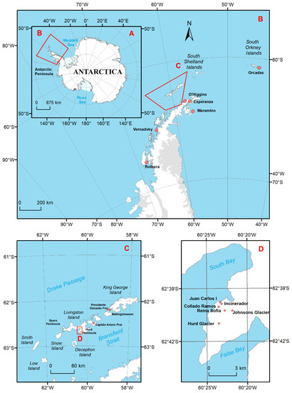
Figure 1.
Location of the Hurd Peninsula of Livingston Island, South Shetland Archipelago, Antarctica (A–D). Location of the AEMET stations and our team’s stations in the Hurd Peninsula.
Livingston Island has a surface area of 974 km2 and is the second island in the extension of the SSI. It has a length of 73 km and a variable width between 5 and 34 km [39]. It is permanently covered by ice in 90% of its surface, and only its west side and some coastal areas are snow-free in the summer. Between these snow-free areas in the summer are the extensive Byers Peninsula (67.5 km2) on the west side and the Hurd and Rozhen Peninsulas in the south. In the Hurd Peninsula, between South Bay and False Bay (Figure 1), the SAS Juan Carlos I has been located since January 1988, at a distance of about 50 m of the western coast of the peninsula and at an elevation of 12 m a.s.l. (above sea level). Behind the observatory, there is a mountainous barrier that almost reaches 300 m next to the SAS and increases its elevation until it reaches the Friesland mountains about 10 km away [39]. Livingston Island in general, and the Hurd Peninsula in particular, is formed by Mesozoic and Cenozoic sedimentary (both detritical and carbonatic), metamorphic, plutonic, and volcanic materials (e.g., [40,41]) affected by tectonic and neotectonics events (e.g., [42,43,44,45]) and modelled by intensive glacial and periglacial processes (e.g., [46,47,48,49,50]), with discontinuous permafrost (e.g., [51]). In the Hurd Peninsula, the AEMET stations Juan Carlos I (JCI), Johnsons Glacier (JG), and Hurd Glacier (HG), and some our team’s stations, are also located (Figure 1).
The daily mean Ta over the year in JCI was −1.2 °C between 1988 and 2014, with a daily mean thermal amplitude of 4.3 °C. This daily mean Ta was 1.9, −0.4, −4.7, and −1.6 °C in summer (December–February; 1987/88–2013/14), autumn (March–May; 1994–2014), winter (June–August; 1994–2014), and spring (September–November; 1994–2014), respectively. The daily mean thermal amplitude was under 4 °C in the summer and autumn and near 5 °C over the rest of the year. The extreme values were between 15.5 °C in the summer and −22.6 °C in the winter. Due to the location of JCI near the sea, the relative humidity is always high, with a mean value of 83% and many times near saturation. The mean pressure is 988.7 hPa, with a maximum of 1032 hPa and a minimum of 942 hPa, both in the winter. The precipitation is higher than 0.1 mm on around 50% of the days, with a mean of 162 days a year, a maximum of 53 days in the summer, and a minimum of 13 days in the winter. The wind is low compared to other stations, with a mean value of 14 km/h, with some lower in summer and higher in winter at 15 km/h. However, the maximum wind velocities range between 50 and 150 km/h over the year, with some extreme cases of 180 km/h [39].
The JG station was designed to study the glacier, so the main data are those of summer and autumn. During the winter, it is buried completely in ice, and the data are no longer representative. The daily mean Ta was 0.2 °C in the summer between 2006/07 and 2014/15 and −2.4 °C in the autumn (2007–2014). The extreme values were between 11.0 °C in the summer and −25.3 °C in the winter. The height of the accumulated snow was close to 2.5 m in these years [39]. The JG station was moved from the Johnsons Glacier to the Hurd Glacier in January 2015, where it is currently, and it has been called the HG station since then.
Our team’s stations, whose Ta values are studied in this article, are Incinerador (INC), Collado Ramos (CR), and Reina Sofía (SOF), around the JCI SAS and near the AEMET stations (Figure 1).
3. Data and Methods
3.1. In Situ Meteorological Stations Ta Data
The in situ Ta data used in this study are the Ta values obtained in the AEMET stations of the Hurd Peninsula (JCI, JG, and HG) and those obtained in three of our monitoring sites in the same peninsula (INC, CR, and RS) (Figure 1). Details of each station (location, height, etc.) as well as the instruments used and the frequency of the data of each station are given in the following subsections. We calculated the daily mean Ta of each station to perform different comparisons.
3.1.1. AEMET Ta Data
The AEMET stations measure the Ta at two different heights over the ground: at 1.80 m and at 20 cm. The Ta at ~2 m is the usual Ta measured at the stations, so it is denoted simply as Ta in most articles, including this one. The Ta at ~20 cm will be denoted as Ta-20cm. Ta is more reliable than Ta-20 cm in our study’s stations, especially in the JG and HG stations, where the sensor at 20 cm is covered with snow most of the year, measuring in these cases the ice temperature or snow temperature near the ground, but not the Ta near the ground (Ta-20 cm). In this regard, in such cold environments, the Ta-20 cm data are not representative when the soil is covered with snow, because they become stable and higher than Ta [52]. Ta will then be used in this article. In Appendix A, we show the comparison between both temperatures when both are reliable (i.e., without snow above 20 cm over the ground, by using the snow cover proxy developed by Bañón et al. [53]), in order to demonstrate that Ta and Ta-20 cm are correlated. The JCI AEMET station started its measurements on the 16 February 1988 using conventional instruments, being open only when the JCI SAS was active, i.e., during the Antarctic summer. In the following year (1989), an automatic weather station (AWS) of the brand SEAC was installed, extending the time period of data collection. An AWS of the brand GEÓNICA was installed in February 2005, collecting data throughout the year. Besides the GEÓNICA AWS of AEMET, in the same meteorological shelter, a Campbell CR10X AWS was installed by other Spanish institution (UTM-CSIC) in January 2001 and was maintained by AEMET, and it is used when the AEMET sensors fail. The first JCI (JCI1) observatory was moved to the current JCI one (JCI2), about 100 m towards the west, on 31 December 2009 [39]. The geographical location (latitude and longitude), height, and operation dates of both JCI observatories are shown in Table 1. In this study, we only used the JCI data collected as of 2000.

Table 1.
Name, location, height above sea level (h), and operation dates of the AEMET stations used in this study.
The JG station is a Campbell CR3000 AWS and was installed in December 2006. As stated in Section 2, this station was moved from the Johnsons Glacier to the Hurd Glacier in January 2015 where it is currently, and it has been known as the HG station since then (Table 1).
The AEMET stations are only maintained when the JCI SAS is active, during the Antarctic summer, four months a year at maximum (from December to March). The data of the entire year are collected in this period. The raw data are usually lacking or bad due to technical problems or very adverse conditions of ice, snow, or wind, so these data are filtered by applying quality control to minimize errors. Since the 2008–2009 campaign, there has been field-calibration equipment (Testotor or Fluke calibrator) for testing the temperature and humidity sensors.
The Ta sensor at JCI, since December 1998, is a Pt100. Brands have changed over the years: HMP45C between December 1998 and March 2005, SRA-5031 between March 2005 and December 2009, and HM45D since 10 December 2009. The Ta-20 cm sensor is also a Pt100: SEAC until February 2007 and GEÓNICA 3012.1850 since March 2007. The data were bad in January 2010, so it was changed on 31 January 2010. The T sensors of the datalogger Campbell CR3000 at JG are Pt100s (HMP45C, changed on 24 December 2009 and on 6 February 2014) and a Thermistor (107 Probe).
The Ta and Ta-20 cm JCI data are obtained every 10 min (10 min) over the entire year, whereas the JG and HG data are obtained every 10 min in the Antarctic summer (December–February) and every half hour (0.5 h) for the rest of the year. The instrumental precision in the temperature measurement is ±0.1 °C with all thermometers and in the three stations [52].
3.1.2. Ta Data in PERMASNOW’s Stations
Our team’s three stations whose Ta values have been analyzed in this study are INC, SOF, and CR. All of them were installed by Miguel Ramos and his group of the University of Alcalá.
The INC station was installed on 25 February 2000 in the same meteorological shelter as that of the JCI AEMET station and remained there until 2005 (INC1). The instrumentation changed over time to improve its capacity and resolution. The first sensors (in 2000 and 2001) were tiny with an internal probe inside the box of the data acquisition systems (DASs), collecting data every 4 h (with an error of ±0.5 °C) and without radiation protection. Tiny DASs collecting data each hour (with errors between ±0.3 °C and ±0.4 °C) with external probes, which are more suitable for Ta measurements, have been used since 2002, and the radiation protector was installed in 2003. In January 2006, the station was moved 300 m from its original location (INC2, Table 2), changing also the Ta sensor height from the ground from 3.0 m to 1.60 m.
Table 2.
Name, location, height above sea level (h), and operation dates of our team’s stations used in this study.
Problems with the instrumentation produced a lack of Ta data at INC between August and November 2001 and in January 2002. On the other hand, a first comparison between the Ta data at INC and JCI during 2000–2005 (when both stations were in the same location) shows that the Ta data at INC in 2000–2001 were highly variable and not reliable, possibly due to the old tiny sensors. Therefore, the Ta data of these two years at INC have been eliminated in this study.
The SOF station was installed on 25 February 2000 on the top of Mount Reina Sofía (Table 2). The instrumentation used in 2000–2004 was the same as that used at INC in those years and similar to that used since 2005 (in both cases, Thermistor or Pt100 sensors). Consequently, the errors in the Ta measurement are ±0.5 °C in 2000–2001 and ±0.3–0.4 °C as of 2002. Several problems with the instrumentation caused a lack of data on most of the days of December 2000 and in other longer periods, such as between 21 March 2001 and 22 February 2002, between 20 September 2004 and 12 January 2005, between 13 January 2010 and 9 January 2011, and between 27 January 2015 and the end of 2015, when the data series of this station used in this study ends. The Ta sensor height above ground is 1.05 m. As at INC, the Ta data from the old tiny sensors do not seem adequate, so we eliminated the data of these two years also at Reina Sofía.
The CR station was installed on the top of an unnamed hill on the 2 February 2006. The Ta sensors are Thermistor or Pt100 sensors, with errors between ±0.3 and 0.4 °C. There were also problems with the instrumentation from 11 January 2010 to 5 January 2011. The Ta sensor height above ground is 1.60 m.
3.2. MODIS Land Surface Temperature Data
We used the MODIS Version 5 (V5) Land Surface Temperature and Emissivity (LST/E) Daily L3 Global 1 km Grid Sinusoidal (SIN) products (MOD11A1.005/MYD11A1.005; MOD refers to a MODIS/Terra product, MYD refers to a MODIS/Aqua product, and 005 refers to the V5) and the MODIS V5 Snow Cover Daily L3 Global 500m Grid (SIN) products (MOD10A1.005/MYD10A1.005). The MOD11A1/MY11A1 products are provided by the NASA Land Processes Distributed Active Archive Center (LP DAAC) [54]. The MOD10A1/MY10A1 products are provided by the NASA National Snow and Ice Data Center (NSIDC) Distributed Active Archive [55,56]. We have obtained these products’ data through the Google Earth Engine (GEE) [57] (http://earthengine.google.org) (accessed on 20 May 2022) Application Programming Interface (API) (https://code.earthengine.google.com/) (accessed on 20 May 2022). The LST/E 1-km resolution values provided by the MOD11A1/MY11A1 products are produced daily using the generalized split-window LST algorithm, based on Band 31 and 32 in the case of the MODIS sensor [58,59], and projected in a SIN grid level-2 (L2) LST/E product. The MOD11A1/MY11A1 products comprise the following Science DataSet (SDS) layers for daytime and nighttime observations: LST, quality control (QC) assessment, observation time, view zenith angle, clear sky coverage, and Band 31 and 32 emissivity values from land cover types. These products include a cloud mask (MOD35/MYD35 product) and a land/water mask (1-km resolution mask contained in the MOD03/MYD03 geolocation product); i.e., there are only LST/E data under clear-sky conditions and in land (included snow, no ice) or inland water [60]. The MOD10A1/MYD10A1 products contain snow cover, snow albedo, fractional snow cover, and quality assessment (QA) data. Snow cover data are based on a snow mapping algorithm that employs a Normalized Difference Snow Index (NDSI) and other criteria tests [56]. These snow cover data also include a classification of the type of cover for each pixel, allowing one to distinguish between snow, land (no snow), water (ocean or inland water (lake)), and cloud. The albedo is only provided if the pixel is classified as snow (snow albedo).
The V5 of the MODIS LST/E products was evaluated by Wan [61] with a comparison between V5 LSTs and in situ Ts values in 47 clear-sky cases (over lakes, silt playa, grasslands, and agricultural fields, and in the LST range from −10 to 58 °C and an atmospheric column water vapor (W) range from 0.4 to 3.5 cm), showing that the accuracy of the V5 MODIS LSTs is apparently better than 1 °C for all but 8 cases with heavy aerosol loadings. Wan [61] also showed that the quantity and quality of MODIS LST products depend on clear-sky conditions because of the inherent limitation of thermal infrared remote sensing. Evaluations of the MODIS LSTs over snow, ice, and permafrost surfaces have been scarce, especially in the Antarctic, and Wan [62] only recently included the South Pole site in his evaluation of the MODIS LST/E products (V6), obtaining an error of −0.5 °C. The V5 MODIS LSTs (at different spatial resolutions) have been evaluated by several authors in the Arctic [30,31,32] and the Antarctic [35], obtaining different results depending on the study area’s location. However, in most cases, the V5 MODIS LSTs underestimated the Ts (i.e., LST < Ts or negative bias). In the Arctic, the mean biases obtained range from −2 to −4 °C during periods with frequent clear-sky conditions (and thus a high density of satellite data), but larger deviations (more than 10 °C) during prolonged cloudy periods prevent satellite measurements, due to an overrepresentation of short colder clear-sky conditions in temporal LST averages [30,31,32]. Regarding the MODIS cloud mask (an integral part of the LST product), the results are contradictory because, whereas Koenig and Hall [30] showed that this mask performed well in their study period and area (winter of 2008/09 at the Summit site, Greenland), Westermann et al. [31,32] (summer and winter time, respectively, at Svalbard, Norway) noted that, in some cases, this mask fails, which leads to strongly erroneous measurements and a systematic negative bias of many more data points, which must be detected and excluded to prevent a considerable bias in the calculated time averages. In Antarctica, Fréville et al. [35] evaluated the V5 MODIS LSTs in 7 stations, 5 of which are located over the Antarctic Plateau and 2 of which are in the northeast coast near the plateau. To minimize cloud detection errors, they selected only the “good quality” or “fairly calibrated” LSTs in their study. They found biases ranging from −2.7 to 0.1 °C, errors (root mean square error, RMSE) ranging from 2.2 to 7.5 °C, and R2 values between 0.69 and 0.97, for a Ts range from −80 to 0 °C. The larger errors were found at coastal stations, whereas in all stations, the regression slope was very close to 1, showing almost no seasonal variability in the LST bias. Fréville et al. [35] also indicated that the coldest biases and the largest RMSEs mainly stem from underestimated LSTs due to the erroneous detection of clear-sky conditions by MODIS.
The MODIS data used in this study range between 5 March 2000/8 July 2002 (Terra/Aqua) and 21 February 2016 (16/14 years). The initial date is determined by the availability of the MODIS LST/E data, whereas the final date is the date of the last AEMET ground meteorological data available for this work, collected in the 2015/2016 Antarctic summer campaign.
LST Filtering
The availability of MODIS LST data in the study area is limited, due to the frequent cloud coverage. Because of this, there are only LST data for as much as 36% of the days in the studied period (27% for the nighttime data), while for the daily mean Ta data, this percentage is 100% (data for SOF, with the longest time period; Table 3). Moreover, the quality of the LST data is variable, and those of the worst quality according to Wan [60] show extremely low temperatures in comparison with Ta (see Appendix C for more details about the quality of the MODIS LST data and the filters applied to these data). In this regard, only the LST data with “good quality” (Appendix C) have been selected, although it reduces significantly the number of points (Table 3). Two filters were applied to these selected LST data using the quality data of the MOD10A1/MYD10A1 products, with a better spatial resolution (500 m) that those of the LST products.
Table 3.
Percentage of days with MODIS LST and Ta data in the time period used in their comparison, and percentage of days with “good” MODIS LST data.
3.3. Methodology
The daily mean Ta was obtained in each meteorological station only in the case that the daily data were complete (n = 144 for the 10 min data, and n = 48 for the 0.5 h data). The first and second locations of the JCI station correspond to the same MODIS pixels. We have analyzed the daily mean Ta values from 1 January 2000 to 21 February 2016. The comparison between the daily mean Ta and the MODIS-LST data (separately for Terra-day, Terra-night, Aqua-day, and Aqua-night) was performed between 5 March 2000/8 July 2002 (Terra/Aqua) and 21 February 2016.
Most analyses performed are based on simple or multiple linear regressions. The statistical computing and graphics were constructed with the free software R (http://www.r-project.org/) (accessed on 29 May 2022) [63]. In all cases, we used robust regressions, models that are less sensitive to outliers, with the MASS library in R [64]. For these models, the statistic parameters used for quantifying the goodness of fit are the square of the correlation coefficient or the coefficient of determination (R2) and the residual standard error (RSE): , where is the value of y predicted by the model, and ν refers to the degrees of freedom, calculated as the total number of observations, n, minus the number of parameters, k (ν = n − 2 in a simple linear regression). As the number of data is low, we have used all of them for constructing the models.
Homogenization of a climatic series is a difficult task that must be performed carefully, especially when metadata are not available [65] and there is a lack of homogeneous stations with raw (not processed) data that can be taken as a reference. Such a task far exceeds the objective of this work and has not been carried out. However, since we want to obtain an approximation of the warming/cooling trends in the studied stations, we have reduced the effect that the change in the locations of JCI and Incinerator (INC) may produce in the temperature time series. Thus, for JCI, we have separately studied the Ta trends in its two locations, JCI1 and JCI2. Moreover, for INC, we have only taken the Ta data from its second and current location (INC2) into account in the Ta trend analysis. JG and HG are already treated separately by the AEMET, and the rest of the stations have not changed their location in the studied temporal period. Regarding the changes or failures in the instrumentation, it is impossible to know how they have affected the Ta, especially in the first decade (2000–2008) when AEMET had no field-calibration equipment for testing its sensors (see Section 3.1.1). Comparing the Ta data of the different stations (Appendix B), we have been able to detect some clear failure in the sensors’ calibration in some years at JCI1 and INC2, so that the Ta of those years has been empirically corrected/homogenized for the Ta trend analysis (Section 4.1) and in the comparison between Ta and LST.
Ta variability over time (t) at each station has been analyzed using two different methods. The first method is a fitting model Ta = f (t) (t in decimal years), which includes t as a variable to define the warming/cooling linear trend and a sine-cosine harmonic (two variables) to take into account the seasonal variation of Ta. This type of model of decomposition in Fourier harmonics is common in analyses of non-stationary time series (e.g., [66]). In our case, the decomposition used is
where the ci parameters are constants. More harmonics (e.g., sin 4t/cos4 have not been necessary, and only the most significant variables, where p-value < 0.05, have been considered in the model.
The second method used to analyze the Ta trend is the robust method LOESS (Locally Weighted Regression) [67,68]. In LOESS, the dependent variable (Ta) is smoothed according to the independent variables (time t) by calculating the value of the regression function for each point in the dataset by evaluating the local polynomial using the values of the explanatory variable (t). For each point, a low-degree polynomial is fitted to a subset of the data using the weighted least squares method, which gives more weight to points closest to the point whose response is being calculated and less weight to the more distant points. The smoothing parameter α’ determines the size of the subset of the data used to adjust each local polynomial. The value of α’ is the proportion of data used in each adjustment and ranges from to 1, where λ is the degree of the local polynomial, and n is the total data in each series analyzed. For our analysis, λ = 2 and α’ = 1. This last value was selected because it produces smoother functions, is less sensitive to data variability, and is therefore more robust in the presence of anomalous values.
A multiple linear regression (MLR) model has been used for estimating Ta for each individual station, which uses LST and the variables used in the linear/harmonic temporal model (1). The structure of the model is
where the ci parameters are constants, and only the variables where p < 0.05 have been considered in the model.
Finally, the global model, for all stations, is also an MLR model that uses the variables in (2) and other spatial variables taking into account the location of the station/point (latitude (φ), longitude (λ), and distance to the coast (d)), its topography (altitude (h), slope (s), curvature (c), and aspect (a)), and its cover type. Topography variables were obtained from the ALOS World 3D (AW3D) DSM, generated using images from the Panchromatic Remote-Sensing Instrument for Stereo Mapping (PRISM) sensor, which is on board the Advanced Land Observing Satellite (ALOS) [69]. In our case, the cover type cannot be described using the Normalized Difference Vegetation Index (NDVI), as is usually done, because there is no vegetation in the study area. The inclusion of these or similar spatiotemporal variables is common in the models of estimation of meteorological variables from MODIS data [28,37,70,71]. The structure of the model is
where the ci parameters are constants.
In the model validation process, we have used the standard leave-one-out cross validation (CV). Statistical parameters include R2CV, the root mean square error (RMSE), , where yobserved is the observed data, and yestimated is the data estimated by a given model (RMSECV in order to indicate the used validation method), the ratio of performance to deviation (RPD), , where σ is the standard deviation of the reference data, and the bias for the mean of the residuals, .
4. Data Analysis and Results
4.1. Ta
The daily mean Ta in the AEMET station JCI shows a behavior of a sinusoidal type. In the other AEMET stations, JG and HG, the sinusoidal behavior is only apparent in the first years at JG (2007–2009) and it is not apparent at HG, in both cases due to a lack of data at the lowest temperatures (Figure 2). Sinusoidal behavior is also found for the daily mean Ta of our three monitoring sites (INC, SOF, and CR; Figure 3).
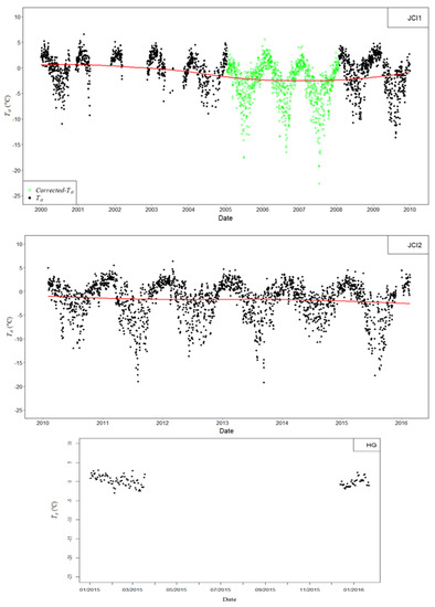
Figure 2.
Daily mean Ta temporal variation for the study period in each AEMET meteorological station (from top to bottom: JCI (first and second location, respectively), JG, and HG). Corrected Ta data are shown in green. The Ta trend obtained with the LOESS method is shown in red on each series. This trend has not been done for the last two years (2014–2015) for JG or for any period for HG, due to the lack of data in these periods.
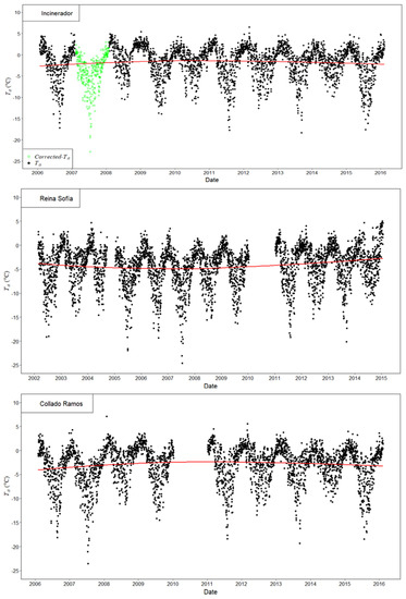
Figure 3.
Daily mean Ta temporal variation for the study period in each meteorological station of our monitoring sites (from top to bottom: INC, SOF, and CR). Corrected Ta data are shown in green. The Ta trend obtained with the LOESS method is shown in red on each series.
Ta data can be unreliable when the snow cover exceeds the height of the Ta sensor, which occurs rarely at JCI, but it could occur at JG and HG. The problem is that there is not a clear criterion for removing unreliable Ta data such as that applied to the unreliable Ta-20 cm data ([52]; Appendix A). In the case of Ta, unreliable data can be removed using the relationship between the Ta values of the stations at different heights (due to the vertical lapse rate), which has been done in Appendix B. These relationships could also be used to expand the data period in some stations (JG, HG, etc.) and/or to fill data gaps, which is not our aim. The results obtained in Appendix B show that it is necessary to remove only three data: one JG datum (24 April 2013), one INC datum (9 September 2013) and one JCI datum (29 January 2008). In Appendix B, we also show the effect of the change in instrumentation and failure in the sensors’ calibration, over the period of study, on the datasets, especially evident at JCI and INC. The unreliable data were corrected empirically, and the variability/linear trends of Ta were determined using the corrected data (the corrected data are shown in green in Figure 2 and Figure 3). Consequently, the following results are with the corrected data. For INC, this is only the case with INC2.
Table 4 shows the fitting model Ta = f (t) (Equation (1)) for JCI, JG, and our three stations. This Ta model yields R2 = 0.51 and RSE = 2.1 °C (with n = 2668) for JCI1 and R2 = 0.47 and RSE = 2.2 °C (with n = 2126) for JCI2, whereas it yields R2 = 0.41 and RSE = 2.0 °C (with n = 1423) for JG. However, it is worth noting that the fit in JG has been done using mainly data of the highest temperatures. The linear trend of the model shows that Ta has decreased slightly at JCI1 (slope, α = −0.15 °C year−1) and JCI2 (α = −0.19 °C year−1), whereas it has remained stable at JG (α = 0 °C year−1) in the time period of the study (Table 4). For our stations, the Ta model is better for CR than for INC2 and SOF. The Ta linear trend is similar for the three stations in the period of study (Table 4). It shows that Ta has increased slightly at CR (α = 0.03 °C year−1), increased slightly at SOF (α = 0.09 °C year−1), and remained stable at INC2 (α = 0 °C year−1).
Table 4.
Results for the daily mean Ta temporal variation in the meteorological stations used in this work: time period, the fitting model Ta = f (t), and the Tinitial, Tfinal, and the ΔTa for the trend obtained with the LOESS method in the time period analyzed in each case. Note that the Ta = f (t) model for JG uses mainly data of the highest temperatures. Since adding a sine wave and a cosine wave of the same frequency (Equation (1)) gives another wave of the same frequency but with a different phase, depending on c3 and c4, in the table, we also present the values of C and φ, obtained analytically from c3 and c4 based on the expression C × sin(2πt + φ), with which the phase φ gives the start of the sine wave.
The LOESS analysis shows similar results to those obtained with the previously made Ta model, confirming that, in the period of study, Ta decreases slightly at JCI1 and JCI2 and increases slightly at the rest of the stations. For the trend obtained with this method, the initial and final Ta (Tini and Tfin, respectively) and the variation of Ta (ΔTa) in the period of the study are also shown in Table 4. These Ta variations, in the standard units of °C decade−1, are −1.5 at JCI1, −2.6 at JCI2, +0.3 at JG, +0.4 at INC2, +0.8 at SOF, and +0.8 at CR.
4.2. Comparison between MODIS LST and Ta
A simple linear regression between Ta and LST of each station gives a low R2 for all stations (R2 ≤ 0.4). R2 improves (Table 5) when using the MLR model of Equation (2) for each station. After applying all the filters, the amount (n) of “good” nighttime data is significantly lower than that of daytime data. A detailed analysis by station shows that, for JCI, the R2 value ranges between 0.4 and 0.7, and the RSE yields around 2 °C. For JG, the R2 value ranges between 0.5 and 0.6, with the exception of that of the Terra-Day data (0.26), and the RSE yields also around 2 °C for the Terra-Day and Aqua-Day data and has a lower value for the Terra-Night data (0.78 °C; n = 6). At this station, no Aqua-Night data were obtained after all filters were applied, so it was not possible to obtain results from the regression model in this case. It was also not possible to obtain results from the model for HG, as no data were available after applying the filters. For CR, the R2 value ranges between 0.6 and 0.7, except for the Terra-Night data (0.36); the RSE varies between 2 and 3 °C in all cases. For INC2, Aqua-Night yields the highest R2 value (0.6). The R2 is 0.5 for the daytime data, and there is a lower value (0.4) for the Terra-Night data, whereas the RSE varies between 2 and 3 °C in all cases. In SOF, the R2 value varies between 0.5 and 0.6 for the daytime data and has a lower value for the Aqua-Night data (0.4), whereas no correlation (0.06) was found for the Terra-Night data; the RSE varies between 2 and 3 °C.
Table 5.
Results of the multiple linear regression for estimating Ta for each station. The structure is with Ta and LST in °C, and t in units of decimal year. Note: * = p-value < 0.1 ⇒ The hypothesis ci = 0 can be rejected at 90% confidence; ** = p-value = 0.16.
In summary, there are a greater number of “good” observations, and, in general, the results are better for the daytime data than for the nighttime data. The R2 value for the daytime data ranges between 0.5 and 0.7, except for JG’s Terra-Day data, possibly due to the low significance of the LST variable in the fit in this case. Except for JG, the number of data is greater, and the results are slightly better when using Terra-Day data (n = 72–139; R2 = 0.5–0.7; RSE = 2 °C) than when using Aqua-Day data (n = 38–98; R2 = 0.5–0.6; RSE = 2–3 °C). The best results using Terra-Day data are obtained, in this order, for CR, JCI2, SOF, and INC2, and the differences among them in terms of R2 and RSE are small.
The results obtained with the best global MLR model for each type of MODIS LST data are shown in Table 6. The fit shows R2 = 0.4–0.6 and RSE = 2–3 °C for n = 116–556. As can be observed, the significant spatial variables (p < 0.05) are curvature, slope, and distance to coast. Figure 4 shows a daily map obtained from this model using the MOD11A1 product of 1 September 2012.
Table 6.
Model for estimating Ta from LST obtained with all data for each type of MODIS LST data. The structure is with Ta and LST in °C, t in decimal year units, curvature (c) in m−1, slope (s) in °, distance to coast (d) in m, and hours of LST observation (H).
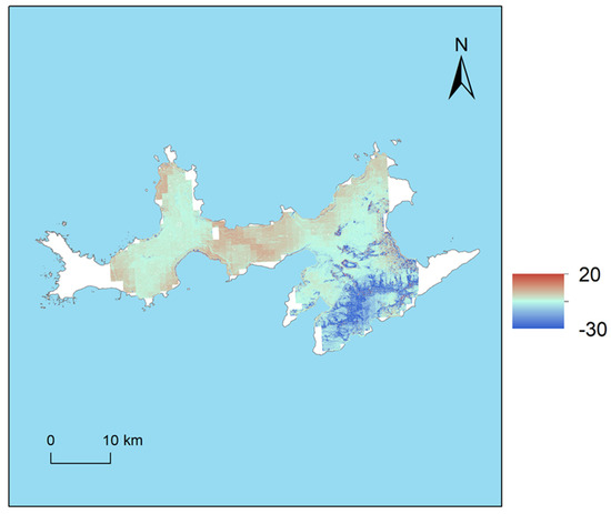
Figure 4.
Ta (°C) obtained with the unique model for Terra-Day generated from the MOD11A1 product including other spatio-temporal variables, from the Terra-MODIS image of 1 September 2012. The area is Livingston Island.
Using a unique model based on all of the in situ data available for each type of MODIS LST data (Terra-Day, Terra-Night, Aqua-Day, and Aqua-Night) and the spatio-temporal variables, the best correlation is obtained for the Terra data. With Terra-Day, R2 (0.6) improves with respect to those obtained in JCI1, JG, and INC2 and are the same as those of JCI2 and SOF, worsening only with respect to CR. Regarding Terra-Night, values (R2 = 0.4) obtained using all of the in situ data are lower than those obtained using data from the stations JCI1 and SOF and equal to those of INC2 and CR. Compared to the Aqua data, the unique model shows very little improvement, with only the Aqua-Night data (R2 = 0.6) improving with respect to JCI1 and SOF.
In terms of the RSE, with Terra-Day data, the unique model yields lower values (RSE = 2.14 °C) than those obtained for the stations JCI1, JG, SOF, and CR. With Terra-Night data, the RSE values (2.10 °C) improve compared to those obtained at the stations JCI1, INC2, and SOF, but they are worse than those obtained at CR. With Aqua-Day data (RSE = 2.7 °C), the results improve only with respect to those of CR, while, with the Aqua-Night data, the unique model only shows lower values of RSE (2.74 °C) than those obtained at the JCI1 station.
5. Validation
Table 7 shows the validation results of the models obtained for the estimation of Ta in each station: R2CV, RMSECV, RPD, and the bias for the mean of the residuals. As expected, the models with the best results in terms of R2 and RSE (Table 5) are those with the best results in the validation, with R2CV and RMSECV only slightly worse than R2 and RSE, respectively (Table 7).
Table 7.
Validation of the models obtained for the estimation of Ta.
In summary, the best results of the validation are, in general, for the daytime models, with R2CV ranging between 0.4 and 0.6 (except for JG) and with RMSECV = 2–3 °C, except for JCI2, where the nighttime data are better. Except for JCI1 and JG, the validation results are better using Terra-Day data than Aqua-Day data. The best results by using Terra-Day data are obtained, in this order, for CR, SOF, JCI2, INC2, and JCI1, although the differences among them are small. According to the classification established by Chang et al. [72], based on the RPD value, in general, the proposed Terra-Day models for these stations can be used to estimate Ta with moderate accuracy (RPD ≥ 1.4).
The validation of the best global MODIS MLR models is shown in Table 8. The R2CV and RMSECV obtained in the validation are slightly lower than the R2 and RSE obtained with the unique model. The validation shows that daytime data are better (R2CV = 0.5; RMSECV = 3 °C; RPD = 1.25–1.41; bias = −0.03) than nighttime data (R2CV = 0.4–0.5; RMSECV = 2–3 °C; RPD = 1.32–1.56; bias = −0.02–0.18). The validation results are slightly better using Terra-Day data (n = 556; R2CV = 0.54; RMSECV = 2.64 °C; RPD = 1.41; bias = −0.03) than Aqua-Day data (n = 406; R2CV = 0.48; RMSECV = 2.97 °C; RPD = 1.25; bias = −0.03).
Table 8.
Validation of the best global MODIS MLR models.
6. Discussion
The results obtained in this study of the daily mean Ta temporal variation between 2000 and 2016 show a complex climatic variability at a spatial scale in the Hurd Peninsula of Livingston Island, similar to that found in other areas of the AP and the SSI (see Section 1). In our case, the stations closer to the coast showed clear cooling trends (with −2.3 °C decade−1 between 2000 and 2009 at JCI1 and −3.0 °C decade−1 between 2010 and 2016 at JCI2), whereas those with a higher altitude had warming trends (with +0.2 °C decade−1 between 2002 and 2016 at INC2 and +0.8 °C decade−1 between 2002 and 2015 and between 2006 and 2016 at SOF and CR, respectively). JG also showed a warming of +0.2 °C decade−1 between 2006 and 2015, although this value is less significant due to data faults. The warming of INC2 is similar to that obtained at the Bellingshausen station (King George Island) between 1948 and 2011 by Kejna et al. [6] and to that estimated by Steig et al. [9] in the West Antarctic’s between 1957 and 2006. On the contrary, the high warming of CR and SOF exceeds even the value found in the AP by O’Donnell et al. [10] between 1957 and 2006 and to the highest trend of +0.54 °C decade−1 for the period 1951–2011 at the Faraday/Vernadsky station found by Turner et al. [7]. In this regard, our study shows that the Faraday station is not an exception, because most of our stations show warming after the year 2000. On the other hand, the cooling rate obtained at JCI1 and JCI2 exceeds the value of −0.47 °C decade−1 obtained by Turner et al. [11] in six coastal stations between 1999 and 2014 and exceeds the cooling by 0.5–0.9 °C between the decades 1996-2005 and 2006-2015 found by Oliva et al. [12] in most of the AP region, with the exception of the SW sector of the AP. The three SSI stations studied by Oliva et al. [12] are localized on King George Island and showed the following annual trends during 2006–2015 (°C year−1): −0.065 at Bellingshausen, −0.022 at Marsh, and +0.041 at King Sejong, i.e., values between −0.65 and +0.41 °C decade−1, although these three results were not significant (p > 0.05). The elevation of these stations is 16, 10, and 11 m, respectively, whereas their mean annual Ta values during 2006–2015 were −2.3, −2.5, and −2.1 °C, respectively. On the other hand, previous studies by our research team indicated a Ta stability trend at both Deception Island (Crater Lake CALM site) between 2006 and 2014 [23] and Livingston Island (Limnopolar Lake CALM site, Byers Peninsula) between 2009 and 2014 [22]. Ramos et al. [23] reported a very stable annual mean Ta at Crater Lake, around −3 °C, between 2006 and 2014; the same stable behavior was found for the maximum and minimum Ta. De Pablo et al. [22] indicated that Ta did not increase at Limnopolar Lake between 2009 and 2014, and only the maximum and mean Ta were slightly reduced (1.6 and 0.5 °C, respectively). In summary, although we studied the daily mean Ta, which is usually more variable than the monthly and annual mean Ta (analyzed in all of the previous studies cited), it seems that the Hurd Peninsula of Livingston Island showed the most extreme Ta cooling/warming rates in the SSI after 2000.
The results of the correlation between the MODIS LST data and the Ta obtained in this study can only be compared with similar previous studies in the coldest areas in the Antarctic, because, to our knowledge, no similar studies have been carried out in the AP and the SSI. The R2 of the linear regression Ta-LST obtained at our stations (R2 ≤ 0.4) is worse than that obtained by Wang et al. [34] from Terra-LST data over the Lambert Glacier Basin, East Antarctica, in the period 2000–2009 (R2 = 0.41–0.98), for eight AWSs with a Ta range from −70 to −15 °C. Our best models (Terra-Day) for estimating Ta from LST and temporal variables yield better results (R2 = 0.5–0.7) than our simplest models, but they are not as good as those obtained by Wang et al. [34], especially in their five East AWSs (R2 ≥ 0.8). On the contrary, the validation of our best models yields a value of RMSECV ≈ 2.5–2.6 °C, against SD values of up to 8.5 °C obtained by Wang et al. [34], i.e., our errors are lower and more stable than those of Wang et al. [34]. Moreover, these authors found an MD between Ta and LST in the range of 2.8–8.1 °C, with an LST lower than the Ta, whereas our bias from −0.1 to 0.1 °C indicates that both temperatures are similar. Our best models (Terra-Day) are also worse in terms of R2CV (0.5–0.6) and better in terms of RMSECV (2.5 °C) than the simple linear model Ta-LST (R2CV = 0.64, RMSECV ≈ 11 °C) and the best machine learning model (GBM: R2CV = 0.71, RMSECV ≈ 11 °C) obtained by Meyer et al. [36] in 2013 taking together the data of 32 stations over the Antarctic continent (with a Ta range from −80 to 10 °C). Meyer et al. [36] also found that the time, in their case the month of the year (2013), was the second predictor after LST in their GMB model to estimate Ta, However, they only probed a simple model Ta-LST as a linear regression model. On the other hand, similar studies on a Pan-Arctic scale show that the correlation Ta-LST is stronger when the temperatures are lower [38]. For example, Urban et al. [33] obtained an R2 of 0.85 for a Ta range from −60 to 0 °C, and an R2 of 0.64 for a Ta range from 0 to 30 °C. This could explain our worse results in terms of R2 against those of Wang et al. [34] and Meyer et al. [36], because our Ta values are much higher (from −25 to 10 °C) than those of these authors.
The unique model improves the results of some stations, increasing the value of R2 and reducing the errors, as they had already shown in a previous study [28]. Thus, the spatial data integration will allow the study to be extended to the entire island and to other areas of the SSI, based on temporal and spatial factors.
7. Conclusions
In this study, we have proposed models to estimate the daily mean Ta in five stations of the Hurd Peninsula of Livingston Island from MODIS-LST data and temporal variables using MRL models. The best Ta models are those generated from the daytime MODIS LST data, those produced with the Terra data (obtained between 10:36 and 13:42 UTC) being better than those produced with the Aqua data (between 16:24 and 19:30 UTC). The models have been obtained empirically and validated using ground-level meteorological stations data and MODIS data between 2000 and 2016. The best results have been obtained in the stations farther from the coast (CR and SOF), although worse results at JCI and INC may be due to changes in the location of the stations and problems in the calibration of the Ta data.
To ensure the reliability of the Ta data in this remote region and the quality of the MODIS data in these cold environments, a detailed study of both types of data was carried out prior to their comparison. The Ta analysis revealed a complex climatic variability at a spatial scale in the Hurd Peninsula between 2000 and 2016, with the station nearest to the coast (JCI1 and JCI2) showing a clear cooling trend in this period (between −1.5 and −2.6 °C decade−1), and with the higher altitude stations showing warming trends (between +0.2 and +0.8 °C decade−1). The study also shows that the Ta data of all used stations are highly reliable and that the data between each station are highly correlated due to the adiabatic gradient. In this regard, the found relationships could help to obtain Ta data at any of these stations when data in some period are missing. Ta is also highly correlated with Ta-20 cm, provided that the unreliable Ta-20 cm data (due to the sensor being covered with snow) has been eliminated. On the other hand, the MODIS LST data only exist in cloud-free days (up to 36% of the studied days), but the main problem is the quality of these data in the Antarctic areas. This study shows that the data with no “good quality” usually underestimate Ta and are not reliable. Therefore, a thorough filtering process was carried out to retain only the “good quality” data, although this filtering drastically reduced the available LST data (at less than 5% of the studied data). However, all months (except June during several years) were represented in this dataset, with more data in April and August and less in June. It is thus concluded that the MODIS-LST data are useful for estimating long-term trends in Ta at a global level (1 km2 spatial resolution) in the Hurd Peninsula of Livingston Island.
Future research will focus on extending the years of study and on analyzing more stations with Ta and LST data in Livingston Island (and/or in other islands of the SSI). In addition, improving the quality of the LST data in this type of cold environment is essential, using new versions of the MODIS LST product or with other sensors. On the other hand, other space–time variables could be added to the models obtained here, such as, NDVI and the type of land cover, which would allow their validity to be studied in other areas that are not covered with snow/ice.
Author Contributions
C.R. designed the study, wrote the article, and edited the majority of it. AEMET air temperature data were analyzed by C.R. and A.C.-P. with contributions from E.P., M.R., M.Á.d.P. and S.F., M.R. and M.Á.d.P. provided the data of our team’s stations, operated in Antarctica since 2009 by M.Á.d.P. Air temperature from our team’s stations was analyzed by C.R., A.C.-P. and M.R. A.C.-P. carried out all the LOESS analyses. MODIS data were obtained and processed by C.R., J.P. and A.C.-P. with contributions from J.F.C. and J.A.C. J.P. obtained the quality codes from the MODIS data to apply the filters. C.R. and A.C.-P. analyzed the MODIS data and compared these data with the air temperature data. A.C.-P. carried out the statistical analysis for obtaining the models for estimating air temperature from MODIS LST data, validated these models, generated the figure and most of the tables, and edited part of the article. M.R. and J.F.C. contributed to the critical analysis of the article. All authors contributed to proofreading and commenting on the manuscript. All authors have read and agreed to the published version of the manuscript.
Funding
This research and the article processing charges (APC) were funded by the Spanish Ministry of Economy and Competitiveness (MINECO) through the PERMASNOW project [CTM2014-52021-R]. C.R., as the coordinator, acknowledges the funds received by the RSApps Research Group from the University of Oviedo in 2018 [PAPI-18-GR-2016-0005]. C.R. also acknowledges the funds for her stay in IGOT (University of Lisbon) from Santander Bank. A.C.-P. acknowledges the following Ph.D. grants: “Severo Ochoa” from the Government of the Principality of Asturias [BP17-151] and the “Predoctoral Grant” from the University of Oviedo.
Data Availability Statement
MODIS data are available in the Google Earth Engine platform (http://earthengine.google.org accessed on 31 May 2022).
Acknowledgments
We would like to thank Manuel Bañón for his help and useful suggestions about the instrumentation and air temperature data of the AEMET stations in the study area. C.R. and A.C.-P. would also like to thank Gonçalo Vieira and the members of his research group for their generous hospitality during their stay in IGOT (University of Lisbon).
Conflicts of Interest
The authors declare that there is no conflict of interest.
Appendix A. Ta and Ta-20 cm
The daily mean Ta and Ta-20 cm in the AEMET stations have similar values and show a similar behavior of sinusoidal type in JCI and JG (2007–2009), varying in phase and with similar amplitude. Figure A1 (included all the data on the left) shows that AEMET Ta and Ta-20 cm are strongly correlated (R2 = 0.80 for JCI and HG, and R2 = 0.66 for JG), the linear slope (α) is ~1, and the RSE is ~1 °C. At JCI, the linear fit Ta versus Ta-20 cm indicates that Ta < Ta-20 cm, but the difference between them (<1 °C) is within the fit error (RSE). For JG and HG, with 10 min and 0.5 h data, the fit using only the daily mean 10 min data (in summer; red color in Figure A1) is better at JG (R2 = 0.78 and RSE < 0.5 °C) than that obtained using all of the data, whereas at HG (R2 = 0.79 and RSE = 0.5 °C), the fit is similar.
Despite the correlation obtained between AEMET Ta and Ta-20 cm when using all of the data, the difference between both temperatures on some days exceeds more than 5 °C at JG or even 10 °C at JCI. These days correspond to stable Ta-20 cm values, between −10 and 0 °C, whereas Ta is between −20 and −10 °C at JCI and between −15 and −5 °C at JG (Figure A1); i.e., Ta is much lower than Ta-20 cm in these cases (Figure A1 on the left). These Ta-20 cm data must be eliminated because they are not reliable, as they correspond to days in which the soil is covered by snow, as stated in Section 3.1.1. This problem is especially visible at JG and confirmed by a much better fit obtained in this station in summer with respect to that obtained with all the data. Thus, we have used the snow cover proxy developed by Bañón et at. [53], based on the analysis of the annual time series of daily standard deviations of Ta-20 cm (σ (Ta-20 cm)), for eliminating Ta-20 cm data when σ (Ta-20 cm) < 0.5 °C. By eliminating these unreliable Ta-20 cm data, the correlation between Ta and Ta-20 cm improves in all stations, especially at JG and JCI, increasing R2 and decreasing RSE (Figure A1 at the right versus Figure A1 at the left).
We conclude that, due to the problems with Ta-20 cm data (these data are irregular, and, moreover, Ta-20 cm is not normalized with a unique standard protocol for all the station, as is Ta), is it better to use Ta data in comparison with MODIS LST data.


Figure A1.
Linear regression between Ta and Ta-20 cm for each AEMET meteorological station: (a) fit with all JCI data, (b) fit with JCI Ta-20 cm data when σ (Ta-20 cm) ≥ 0.5 °C, (c) fit with all JG data, (d) fit with JG Ta-20 cm data when σ (Ta-20 cm) ≥ 0.5 °C, (e) fit with all HG data, (f) fit with HG Ta-20 cm data when σ (Ta-20 cm) ≥ 0.5 °C. In red with only the summer data (10 min) at JG and HG.


Appendix B. Comparison between Ta of Different Stations: Correction of the Bad Calibrated Ta Data
The relationships between Ta of the stations at different heights (due to the vertical lapse rate) have been used, in our case, to correct or remove Ta unreliable data. However, in other cases, they could also be used to expand the data period in some stations (for example, JG, HG, and CR; see Figure 2 and Figure 3) and/or to obtain lacking data. Because the position of the JCI station changed (JCI1 in 2000–2009 and JCI2 in 2010–2016), it was necessary to separate the data of both locations in the analysis. Regarding JCI2 versus the rest of the stations (Figure A2, JCI2 in red), all correlations are very good (R2 = 0.89–0.99). In the case of JCI1, except for JG (R2 = 0.92), these correlations decrease (R2 = 0.79–0.89) (Figure A2, JCI1 in black) and JCI1 data are split into two parallel lines, clearly differentiated in the comparison with INC, SOF, and CR. Given that the highest separability between the lines is obtained in the comparison with CR (between 2006 and 2009), this one has been used to find and correct the bad calibrated data in the period 2006–2009 in JCI1, assuming that some failure in the sensors’ calibration is the cause of the difference between both lines. CR-Ta versus JCI1-Ta is shown in Figure A3 (at the left), where it can be observed that the intercept of the linear fit is clearly lower for the bad calibrated JCI1 data (from 2 February 2006 to 28 January 2008) than for the good calibrated JCI1 data (from 1 February 2008 to 30 December 2009) (whereas the slope of the fit is similar, α≈1), indicating a higher Ta at the bad calibrated data than those of the good calibrated ones, for the same value of Ta at CR. Combining the fits of both lines (and assuming the same slope, α≈1), the following Equation (A1) has been obtained for correcting the bad calibrated data (since 2 February 2006 until 28 January 2008) in JCI1:
Corrected JCI1-Ta (°C) = Bad calibrated JCI1-Ta (°C) −2.47 °C
The result of the correction is shown in Figure A3 (at the right).
A similar strategy has been applied to correct the bad calibrated JCI1 data prior to 2 February 2006, using INC-Ta versus JCI1-Ta (when they were in the same location). The comparison shows the best separability between the lines after those with CR. The results are shown in Figure A4. In this case, Equation (A2) is obtained for correcting the bad calibrated data from 14 January 2005 to 1 February 2006:
Corrected JCI1-Ta (°C) = Bad calibrated JCI1-Ta (°C) −2.28 °C
Comparing Equation (A1) and (A2), it can be observed than the difference between the correction factor in both cases is low (0.19 °C) and is within the errors of the Ta sensors at the INC and CR stations (±0.3–0.4 °C; see Section 3.1.2). In summary, the problem seems to be the change of instrumentation and sensors in 2005 and the lack of calibration parameters until 2008 at JCI1 [52] (see Section 3.1.1). On the contrary, the change of location from JCI1 to JCI2 does not seem to affect the Ta data, although both locations have been analyzed separately.
Figure A5 shows the comparison between our team’s highest stations, SOF (h = 271 m) and CR (h = 117 m), with the Ta of our lowest station, INC (12 m in its first location, INC1, in the period between 2000 and 20 January 2006, and 34 m in its second location, INC2, since 23 January 2006). The comparison between SOF and INC is between 2000 and 2016, and a high dispersion is observed in the fit, which does not allow one to find bad calibrated INC data. On the contrary, in the comparison between CR and INC2 (since 2 February 2006), two parallel lines can be observed again, indicating bad calibrated INC2 data between 13 February 2007 and 28 January 2008). In this case, Equation (A3) is obtained for correcting the bad calibrated INC2 data:
Corrected INC2-Ta (°C) = Bad calibrated INC2-Ta (°C) −2.07 °C

Figure A2.
Linear regression between Ta of the stations at different heights and JCI. (a) JG (h = 178 m), (b) INC (h = 12–34 m), (c) SOF (h = 271 m) and (d) CR (h = 117 m) versus JCI-Ta (h = 12–13 m). JCI1 and JCI2 refer to the first and the second location of JCI, respectively.
Figure A2.
Linear regression between Ta of the stations at different heights and JCI. (a) JG (h = 178 m), (b) INC (h = 12–34 m), (c) SOF (h = 271 m) and (d) CR (h = 117 m) versus JCI-Ta (h = 12–13 m). JCI1 and JCI2 refer to the first and the second location of JCI, respectively.


Figure A3.
Linear regression between CR-Ta and JCI1-Ta: (a) with the original JCI1 data, (b) after applying the correction of Equation (A1) to the bad calibrated (in green) JCI1 data.
Figure A3.
Linear regression between CR-Ta and JCI1-Ta: (a) with the original JCI1 data, (b) after applying the correction of Equation (A1) to the bad calibrated (in green) JCI1 data.


Figure A4.
(a) Linear regression between INC-Ta and JCI1-Ta when they were in the same location: with the original JCI1 data, (b) after applying the correction of Equation (A2) to the bad calibrated (in green) JCI1 data, (c) Linear regression between INC-Ta and JCI1-Ta with all data.
Figure A4.
(a) Linear regression between INC-Ta and JCI1-Ta when they were in the same location: with the original JCI1 data, (b) after applying the correction of Equation (A2) to the bad calibrated (in green) JCI1 data, (c) Linear regression between INC-Ta and JCI1-Ta with all data.


Figure A5.
(a) Linear regression between Ta of SOF versus INC, (b) Linear regression between Ta of CR versus original INC2 data, (c) Linear regression between Ta of CR versus INC2 data after applying the correction of Equation (A3) to the bad calibrated INC2 data. INC1 and INC2 refer to the first and the second location of INC, respectively.

Finally, considering the clearly bad data to be removed, which is the other aim of the comparison between the Ta values of different stations, from Figure A2, it seems that it is necessary to remove three data: one datum measured in the JG station, corresponding to 24 April 2013 (autumn), with a low Ta value in comparison with that of JCI (JCI2), one datum measured in INC, corresponding to 9 September 2013 with a high Ta value in comparison with that of JCI2 (also seen in the fit of CR-INC from Figure A4), and one datum corresponding to 29 January 2008 in JCI1, between the bad calibrated and good calibrated JCI1 data.
Appendix C. Quality of the MODIS LST Data and Applied Filters
The quality of the LST data is variable, and those of the worst quality according to Wan [60] show extremely low temperatures in comparison with Ta (Table A1 and Figure A6a). In this regard, only the LST data with “good quality” (QC code = 00000000; see Table A1) have been selected, although this significantly reduces the number of points (see Figure A6a,b for JCI1 and Terra-Day data as an example).
Table A1.
QC codes of our MODIS LST data (they are read from the right to the left in groups of two numbers), their key or explanation from Wan (2006), and the color of the points with each code in Figure A6.
Table A1.
QC codes of our MODIS LST data (they are read from the right to the left in groups of two numbers), their key or explanation from Wan (2006), and the color of the points with each code in Figure A6.
| LST QC Codes (Read ←) | Key (from Wan (2006); Table 14) | Point Color in Figure A6 |
|---|---|---|
| 00000010 | 10 = LST not produced due to cloud effects | -(No data) |
| 11000101 | 01 = LST produced, other quality, recommend examination of more detailed QA 01 = other quality data 00 = average emissivity error <= 0.01 11 = average LST error > 3 K | Blue |
| 10000101 | 10 = average LST error <= 3 K | Brown |
| 01000101 | 01 = average LST error <= 2 K | Green |
| 01000001 | 00 = good data quality 01 = average LST error <= 2 K | Orange |
| 00000101 | 01 = other quality data 00 = average LST error <= 1 K | - |
| 00000000 | 00 = LST produced, good quality, not necessary to examine more detailed QA | Pink |
On the other hand, considering the QA of the MOD10A1/MYD10A1 products for the LST data selected, and the “Snow_Spatial_QA_Description” in particular (SS_QA_D), we have also decided to remove the data with “Other quality” in this description (see Figure A6b). This is due to the fact that these “Other quality” data seem to produce only “noise” in the relationship between Ta and LST, although in our case there are few points of this type in comparison with the rest of the points, so they do not influence the final result in terms of R2 much. On the contrary, the data with SS_QA_D = “Ocean mask” have been maintained, because they surely correspond to days of the year when the snow is mostly melted in the studied locations. The rest of the data have SS_QA_D = “Good quality” (Figure A6b). However, these “Good quality” data are divided in several groups according to other descriptions; for example, in our case, the most interesting is the “Snow_Cover_Daily_Tile_Descrip” (S_C_D_T_D), which divides our “Good quality” data into “Cloud obscured,” “Snow-covered land,” and “Snow-free land” (Figure A6c). In this regard, the “Cloud obscured” data have been also removed, because they were not detected as cloudy in the 1 km LST products, but they were in these snow products with a 500 m spatial resolution. In our case, however, they are few data, and they hardly influence the final result in terms of R2. With respect to the snow-covered and snow-free land data, its relationship Ta versus LST is similar (and these data are similar to the open-water (melted snow) data), so all have been taken together in the analysis of each station (Figure A6d). In the global model, these three covers have been considered, but the cover type is not significant.

Figure A6.
Relationship between the daily mean Ta and the diurnal LST from Terra-MODIS at JCI1 (station shown as an example). The different panels show the successive filters applied to the MODIS data: (a) All MODIS data before filtering; see the QC codes for each color in Table A1. (b) Data after applying the QC filter, separated by the SS_QA_D. (c) Data after removing the “Other quality” data in SS_QA_D, separated by the S_C_D_T_D. (d) “Good” data after removing the “Cloud obscured” data in S_C_D_T_D. In summary, after removing “bad” LST data, we have only “good” LST data for as much as 4% of the studied days (1% for the nighttime data) (see Table 3 in the main text).

References
- Turner, J.; Colwell, S.R.; Marshall, G.J.; Lachlan-Cope, T.A.; Carleton, A.M.; Jones, P.D.; Lagun, V.; Reid, P.A.; Iagovkina, S. Antarctic climate change during the last 50 years. Int. J. Climatol. 2005, 25, 279–294. [Google Scholar] [CrossRef]
- King, J.C. Recent climate variability in the vicinity of the Antarctic Peninsula. Int. J. Climatol. 1994, 14, 357–369. [Google Scholar] [CrossRef]
- Marshall, G.J.; Lagun, V.; Lachlan-Cope, T.A. Changes in Antarctic Peninsula tropospheric temperatures from 1956 to 1999: A synthesis of observations and reanalysis data. Int. J. Climatol. 2002, 22, 291–310. [Google Scholar] [CrossRef]
- Vaughan, D.; Marshall, G.; Connolley, W.; Parkinson, C.; Mulvaney, R.; Hodgson, D.; King, J.; Pudsey, C.; Turner, J. Recent rapid regional climate warming on the Antarctic Peninsula. Clim. Chang. 2003, 60, 243–274. [Google Scholar] [CrossRef]
- Stastna, V. Spatio-temporal changes in surface air temperature in the region of the northern Antarctic Peninsula and South Shetland Islands during 1950–2003. Polar Sci. 2010, 4, 18–33. [Google Scholar] [CrossRef]
- Kejna, M.; Araźny, A.; Sobota, I. Climatic change on King George Island in the years 1948–2011. Pol. Polar Res. 2013, 34, 213–235. [Google Scholar] [CrossRef]
- Turner, J.; Barrand, N.E.; Bracegirdle, T.J.; Convey, P.; Hodgson, D.A.; Jarvis, M.; Jenkins, A.; Marshall, G.; Meredith, M.P.; Roscoe, H.; et al. Antarctic climate change and the environment: An update. Polar Rec. 2014, 50, 237–259. [Google Scholar] [CrossRef]
- Vaughan, D.G.; Comiso, J.C.; Allison, I.; Carrasco, J.; Kaser, G.; Kwok, R.; Mote, P.; Murray, T.; Paul, F.; Ren, J.; et al. Observations: Cryosphere. In Climate Change 2013: The Physical Science Basis. Contribution of Working Group I to the Fifth Assessment Report of the Intergovernmental Panel on Climate Change; Stocker, T.F., Qin, D., Plattner, G.-K., Tignor, M., Allen, S.K., Boschung, J., Nauels, A., Xia, Y., Bex, V., Midgley, P.M., Eds.; Cambridge University Press: Cambridge, UK; New York, NY, USA, 2013; pp. 317–382. [Google Scholar]
- Steig, E.J.; Schneider, D.P.; Rutherford, S.D.; Mann, M.E.; Comiso, J.C.; Shindell, D.T. Warming of the Antarctic ice-sheet surface since the 1957 International Geophysical Year. Nature 2009, 457, 459–462. [Google Scholar] [CrossRef]
- O’Donnell, R.; Lewis, N.; McIntyre, S.; Condon, J. Improved Methods for PCA-Based Reconstructions: Case Study Using the Steig et al. (2009) Antarctic Temperature Reconstruction. J. Clim. 2011, 24, 2099–2115. [Google Scholar] [CrossRef]
- Turner, J.; Lu, H.; White, I.; King, J.C.; Phillips, T.; Hosking, J.S.; Bracegirdle, T.J.; Marshall, G.J.; Mulvaney, R.; Deb, P. Absence of 21st century warming on Antarctic Peninsula consistent with natural variability. Nature 2016, 535, 411–415. [Google Scholar] [CrossRef] [PubMed]
- Oliva, M.; Navarro, F.; Hrbáček, F.; Hernández, A.; Nývlt, D.; Pereira, P.; Ruiz-Fernández, J.; Trigo, R. Recent regional climate cooling on the Antarctic Peninsula and associated impacts on the cryosphere. Sci. Total Environ. 2017, 580, 210–223. [Google Scholar] [CrossRef]
- Salomonson, V.V.; Barnes, W.L.; Maymon, P.W.; Montgomery, H.E.; Ostrow, H. MODIS: Advanced Facility Instrument for Studies of the Earth as a System. IEEE Trans. Geosci. Remote Sens. 1989, 27, 145–153. [Google Scholar] [CrossRef]
- Ramos, M. Automatic device to measure the active permafrost layer near the Spanish Antarctic Station. Terra Antarct. 1995, 2, 61–63. [Google Scholar]
- Ramos, M. Topographic Distribution of Short-wave Radiation in the surroundings of the Spanish Antarctic Station Austral summers. Terra Antart. 1997, 4, 5–10. [Google Scholar]
- Ramos, M. Active Layer in the vicinity of the Spanish Antarctic Station. Terra Antart. 1998, 5, 189–193. [Google Scholar]
- Ramos, M.; Vieira, G.; Blanco, J.J.; Gruber, S.; Hauck, C.; Hidalgo, M.A.; Tome, D. Thermal active layer monitoring in two different sites on Livingston Island during the last seven years: A comparative study. In Proceedings of the Ninth International Conference on Permafrost, Fairbanks, AK, USA, June 29–July 3 2008; pp. 1463–1467. [Google Scholar]
- Ramos, M.; Hasler, A.; Vieira, G.; Hauck, C.; Gruber, S. Drilling and installation of boreholes for permafrost thermal monitoring on Livingston Island in the maritime Antarctic. Permafr. Periglac. Processes 2009, 20, 57–64. [Google Scholar] [CrossRef]
- Vieira, G.; Bockheim, J.; Guglielmin, M.; Balks, M.; Abramov, A.A.; Boelhouwers, J.; Cannone, N.; Ganzert, L.; Gilichinsky, D.A.; Goryachkin, S.; et al. Thermal State of Permafrost and Active-layer Monitoring in the Antarctic: Advances During the International Polar Year 2007-2009. Permafr. Periglac. Processes 2010, 21, 182–197. [Google Scholar] [CrossRef]
- de Pablo, M.A.; Blanco, J.J.; Molina, A.; Ramos, M.; Quesada, A.; Vieira, G. Interannual active layer variability at the Limnopolar Lake CALM site on Byers Peninsula, Livingston Island, Antarctica. Antarct. Sci. 2013, 25, 167–180. [Google Scholar] [CrossRef]
- de Pablo, M.A.; Ramos, M.; Molina, A. Thermal characterization of the active layer at the Limnopolar Lake CALM-S site on Byers Peninsula (Livingston Island), Antarctica. Solid Earth 2014, 5, 721–739. [Google Scholar] [CrossRef]
- de Pablo, M.A.; Ramos, M.; Molina, A. Snow cover evolution, on 2009-2014, at the Limnopolar Lake CALM-S site on Byers Peninsula, Livingston Island, Antarctica. Catena 2017, 149, 538–547. [Google Scholar] [CrossRef]
- Ramos, M.; Vieira, G.; de Pablo, M.A.; Molina, A.; Abramov, A.; Goyanes, G. Recent shallowing of the thaw depth at Crater Lake, Deception Island, Antarctica (2006–2014). Catena 2017, 149, 519–528. [Google Scholar] [CrossRef]
- De Pablo, M.A.; Ramos, M.; Molina, A.; Vieira, G.; Hidalgo, M.A.; Prieto, M.; Jiménez, J.J.; Fernández, S.; Recondo, C.; Calleja, J.F.; et al. Frozen ground and snow cover monitoring in the South Shetland Islands, Antarctica: Instrumentation, effects on ground thermal behaviour and future research. Cuad. Investig. Geográfica 2016, 42, 475–495. [Google Scholar] [CrossRef]
- De Pablo, M.A.; Jiménez, J.J.; Ramos, M.; Prieto, M.; Molina, A.; Vieira, G.; Hidalgo, M.A.; Fernández, S.; Recondo, C.; Calleja, J.F.; et al. Frozen Ground and Snow Cover Monitoring in Livingston and Deception Islands, Antarctica: Preliminary Results of the-PERMASNOW Project. Cuad. Investig. Geográfica 2020, 46, 187–222. [Google Scholar] [CrossRef]
- Calleja, J.F.; Corbea-Pérez, A.; Fernández, S.; Recondo, C.; Peón, J.; de Pablo, M.Á. Snow Albedo Seasonality and Trend from MODIS Sensor and Ground Data at Johnsons Glacier, Livingston Island, Maritime Antarctica. Sensors 2019, 19, 3569. [Google Scholar] [CrossRef]
- Corbea-Pérez, A.; Calleja, J.F.; Recondo, C.; Fernández, S. Evaluation of the MODIS (C6) Daily Albedo Products for Livingston Island, Antarctic. Remote Sens. 2021, 13, 2357. [Google Scholar] [CrossRef]
- Recondo, C.; Peón, J.J.; Zapico, E.; Pendás, E. Empirical models for estimating daily surface water vapour pressure, air temperature, and humidity using MODIS and spatiotemporal variables. Applications to peninsular Spain. Int. J. Remote Sens. 2013, 34, 8051–8080. [Google Scholar] [CrossRef]
- Hall, D.; Box, J.; Casey, K.; Hook, S.; Shuman, C.; Steffen, K. Comparison of satellite-derived and in-situ observations of ice and snow surface temperatures over Greenland. Remote Sens. Environ. 2008, 112, 3739–3749. [Google Scholar] [CrossRef]
- Koenig, L.S.; Hall, D.K. Comparison of satellite, thermochron and air temperatures at Summit, Greenland, during the winter of 2008/09. J. Glaciol. 2010, 56, 735–741. [Google Scholar] [CrossRef]
- Westermann, S.; Langer, M.; Boike, J. Spatial and temporal variations of summer surface temperatures of high-arctic tundra on Svalbard—Implications for MODIS LST based permafrost monitoring. Remote Sens. Environ. 2011, 115, 908–922. [Google Scholar] [CrossRef]
- Westermann, S.; Langer, M.; Boike, J. Systematic bias of average winter-time land surface temperatures inferred from MODIS at a site on Svalbard, Norway. Remote Sens. Environ. 2012, 118, 162–167. [Google Scholar] [CrossRef]
- Urban, M.; Eberle, J.; Hüttich, C.; Schmullius, C.; Herold, M. Comparison of Satellite-Derived Land Surface Temperature and Air Temperature from Meteorological Stations on the Pan-Arctic Scale. Remote Sens. 2013, 5, 2348–2367. [Google Scholar] [CrossRef]
- Wang, Y.; Wang, M.; Zhao, J. A Comparison of MODIS LST Retrievals with in Situ Observations from AWS over the Lambert Glacier Basin, East Antarctica. Int. J. Geosci. 2013, 04, 611–617. [Google Scholar] [CrossRef]
- Fréville, H.; Brun, E.; Picard, G.; Tatarinova, N.; Arnaud, L.; Lanconelli, C.; Reijmer, C.; van den Broeke, M. Using MODIS land surface temperatures and the Crocus snow model to understand the warm bias of ERA-Interim reanalyses at the surface in Antarctica. Cryosph. 2014, 8, 1361–1373. [Google Scholar] [CrossRef]
- Meyer, H.; Katurji, M.; Appelhans, T.; Müller, M.U.; Nauss, T.; Roudier, P.; Zawar-Reza, P. Mapping Daily Air Temperature for Antarctica Based on MODIS LST. Remote Sens. 2016, 8, 732. [Google Scholar] [CrossRef]
- Peón, J.; Recondo, C.; Calleja, J.F. Improvements in the estimation of daily minimum air temperature in peninsular Spain using MODIS land surface temperature. Int. J. Remote Sens. 2014, 35, 5148–5166. [Google Scholar] [CrossRef]
- Hachem, S.; Duguay, C.R.; Allard, M. Comparison of MODIS-derived land surface temperatures with ground surface and air temperature measurements in continuous permafrost terrain. Cryosphere 2012, 6, 51–69. [Google Scholar] [CrossRef]
- Bañón, M.; Vasallo, F. Aemet en la Antártida. Climatología y Meteorología Sinóptica en Las Estaciones Meteorológicas en Las Estaciones Meteorológicas Españolas en la Antártida; AEMET: Madrid, Spain, 2015.
- Hobbs, G.J. The Geology of the South. Shetland Islands: IV. The Geology of Livingston Island; British Antarctic Survey: London, UK, 1968; Volume 47. [Google Scholar]
- Smellie, J.L.; Pankhurst, R.; Thomson, M.R.A.; Davies, R.E.S. The Geology of the South Shetland Islands: VI. Stratigraphy, Geochemistry and Evolution; British Antarctic Survey: Cambridge, UK, 1984; Volume 87, ISBN 0856651087. [Google Scholar]
- Tokarski, A.K. The Late Cretaceous-Cenozoic structural history of King George Island, South Shetland Islands, and its plate-tectonic setting. In Geological Evolution of Antarctica; Thomson, M.R., Crame, J., Thomson, J., Eds.; Cambridge University Press: Cambridge, UK, 1991; pp. 493–497. [Google Scholar]
- Santanach, P.; Pallás, R.; Sàbat, F.; Muñoz, J. La fracturación en la Isla Livingston, Islas Shetland del Sur. In Simposios: III Congreso geológico de España y VIII Congreso Latinoamericano de Geología; Universidad de Salamanca: Salamanca, Spain, 1992; pp. 141–151. [Google Scholar]
- Willan, R.C.R. Preliminary field observations on peperites and hydrothermal veins and breccias on Livingston Island, South Shetland Islands. Antarct. Sci. 1992, 4, 109–110. [Google Scholar] [CrossRef]
- Willan, R.C.R. Structural setting and timing of hydrothermal veins and breccias on Hurd Peninsula, South Shetland Islands: A possible volcanic-related epithermal system in deformed turbidites. Geol. Mag. 1994, 131, 465–483. [Google Scholar] [CrossRef]
- López-Martínez, J.; Martinez de Pison, E.; Arche, A. Geomorphology of Hurd Peninsula, Livingston Island, South Shetland Islands. In Recent Progress in Antarctic Earth Science; Yoshida, Y., Kaminuma, K., Shiraishi, K., Eds.; Terrapub: Tokyo, Japan, 1992; pp. 751–756. [Google Scholar]
- López-Martínez, J.; Vilaplana, J.; Martínez de Pisón, E.; Calvet, J.; Arche, A.; Serrat, D.; Pallàs, R. Geomorphology of selected areas in Livingston Island, South Shetland Islands. In Simposios: III Congreso geológico de España y VIII Congreso Latinoamericano de Geología. Vol. 3: Geología de la Antártida Occidental.; López-Martínez, J., Ed.; Universidad de Salamanca: Salamanca, Spain, 1992; pp. 271–281. ISBN 84-600-8114-1. [Google Scholar]
- López-Martínez, J.; Serrano, E.; Schmid, T.; Mink, S.; Linés, C. Periglacial processes and landforms in the South Shetland Islands (northern Antarctic Peninsula region). Geomorphology 2012, 155, 62–79. [Google Scholar] [CrossRef]
- Lopez-Martinez, J.; Schmid, T.; Serrano, E.; Mink, S.; Nieto, A.; Guillaso, S. Geomorphology and surface landforms distribution in selected ice-free areas in the South Shetland Islands, Northern Antarctic Peninsula region. Cuad. Investig. Geográfica 2016, 42, 435–455. [Google Scholar] [CrossRef][Green Version]
- Pallàs, R.; Vilaplana, J.M.; Sàbat, F. Geomorphological and neotectonic features of Hurd Peninsula, Livingston Island, South Shetland Islands. Antarct. Sci. 1995, 7, 395–406. [Google Scholar] [CrossRef]
- Bockheim, J.G. Permafrost distribution in the southern circumpolar region and its relation to the environment: A review and recommendations for further research. Permafr. Periglac. Processes 1995, 6, 27–45. [Google Scholar] [CrossRef]
- Bañón, M. Personal Communication; AEMET: Madrid, Spain, 2017.
- Bañón, M.; Justel, A.; Velázquez, D.; Quesada, A. Regional weather survey on Byers Peninsula, Livingston Island, South Shetland Islands, Antarctica. Antarct. Sci. 2013, 25, 146–156. [Google Scholar] [CrossRef]
- NASA LP DAAC, 2016, MODIS Land Surface Temperature and Emissivity (LST/E) Daily L3 Global 1 km Grid SIN Products (MOD11A1.005/MYD11A1.005). Version 5. NASA EOSDIS Land Processes DAAC, USGS Earth Resources Observation and Science (EROS) Center. Available online: https://lpdaac.usgs.gov/dataset_discovery/modis/modis_products_table/mod11a1 (accessed on 20 April 2018).
- NASA NSIDC, 2016, MODIS Snow Cover Daily L3 Global 500 m Grid (MOD10A1.005/MYD10A1.005). Version 5.NASA National Snow and Ice Data Center Distributed Active Archive (NSIDC). Available online: http://nsidc.org/data/docs/daac/modis_v5/mod10a1_modis_terra_snow_daily_global_500m_grid.gd.html (accessed on 20 April 2018).
- Hall, D.K.; Salomonson, V.V.; Riggs, G.A. MODIS Snow Products. User Guide to Collection 5; NASA: National Snow and Ice Data Center Distributed Active Archive Center: Washington, DC, USA, 2006. [Google Scholar]
- Gorelick, N.; Hancher, M.; Dixon, M.; Ilyushchenko, S.; Thau, D.; Moore, R. Google Earth Engine: Planetary-scale geospatial analysis for everyone. Remote Sens. Environ. 2017, 202, 18–27. [Google Scholar] [CrossRef]
- Wan, Z.; Dozier, J. A generalized split-window algorithm for retrieving land-surface temperature from space. IEEE Trans. Geosci. Remote Sens. 1996, 34, 892–905. [Google Scholar] [CrossRef]
- Wan, Z. MODIS Land-Surface Temperature Algorithm Theoretical Basis Document (LST ATBD, Version 3.3). Available online: http://modis.gsfc.nasa.gov/data/atbd/atbd_mod11.pdf (accessed on 20 April 2018).
- Wan, Z. Collection-5. MODIS Land Surface Temperature Products Users’ Guide, September 2006. Available online: http://www.icess.ucsb.edu/modis/LstUsrGuide/MODIS_LST_products_Users_guide_C5.pdf (accessed on 20 April 2018).
- Wan, Z. New refinements and validation of the MODIS Land-Surface Temperature/Emissivity products. Remote Sens. Environ. 2008, 112, 59–74. [Google Scholar] [CrossRef]
- Wan, Z. New refinements and validation of the collection-6 MODIS land-surface temperature/emissivity product. Remote Sens. Environ. 2014, 140, 36–45. [Google Scholar] [CrossRef]
- Crawley, M.J. The R Book; John Wiley & Sons, Ltd.: Chichester, UK, 2007; ISBN 978-047051024-7. [Google Scholar]
- Venables, W.N.; Ripley, B.D. Modern Applied Statistics with S, 4th ed.; Springer: New York, NY, USA, 2002; ISBN 0-387-95457-0. [Google Scholar]
- Toreti, A.; Kuglitsch, F.G.; Xoplaki, E.; Della-Marta, P.M.; Aguilar, E.; Prohom, M.; Luterbacher, J. A note on the use of the standard normal homogeneity test to detect inhomogeneities in climatic time series. Int. J. Climatol. 2011, 31, 630–632. [Google Scholar] [CrossRef]
- Jenkins, G.M.; Watts, D.G. Spectral Analysis and Its Applications, 5th ed.; Emerson-Adams Press: Boca Raton, FL, USA, 1998. [Google Scholar]
- Cleveland, W.S. Robust Locally Weighted Regression and Smoothing Scatterplots. J. Am. Stat. Assoc. 1979, 74, 829–836. [Google Scholar] [CrossRef]
- Cleveland, W.S.; Devlin, S.J. Locally weighted regression: An approach to regression analysis by local fitting. J. Am. Stat. Assoc. 1988, 83, 596–610. [Google Scholar] [CrossRef]
- Earth Obervation Research Center JAXA ALOS Global Digital Surface Model “ALOS World 3D—30m (AW3D30)”. Available online: https://www.eorc.jaxa.jp/ALOS/en/dataset/aw3d30/aw3d30_e.htm (accessed on 21 June 2021).
- Kang, J.; Tan, J.; Jin, R.; Li, X.; Zhang, Y. Reconstruction of MODIS Land Surface Temperature Products Based on Multi-Temporal Information. Remote Sens. 2018, 10, 1112. [Google Scholar] [CrossRef]
- Benali, A.; Carvalho, A.C.; Nunes, J.P.; Carvalhais, N.; Santos, A. Estimating air surface temperature in Portugal using MODIS LST data. Remote Sens. Environ. 2012, 124, 108–121. [Google Scholar] [CrossRef]
- Chang, C.; Laird, D.; Mausbach, M.; Hurburgh, C. Near-Infrared Reflectance Spectroscopy–Principal Components Regression Analyses of Soil Properties. Soil Sci. Soc. Am. J. 2001, 65, 480–490. [Google Scholar] [CrossRef]


Publisher’s Note: MDPI stays neutral with regard to jurisdictional claims in published maps and institutional affiliations. |
© 2022 by the authors. Licensee MDPI, Basel, Switzerland. This article is an open access article distributed under the terms and conditions of the Creative Commons Attribution (CC BY) license (https://creativecommons.org/licenses/by/4.0/).