
The Role of Soil Salinization in Shaping the Spatio-Temporal Patterns of Soil Organic Carbon Stock


 ,
,  ,
, 

Abstract
:1. Introduction
2. Materials and Methods
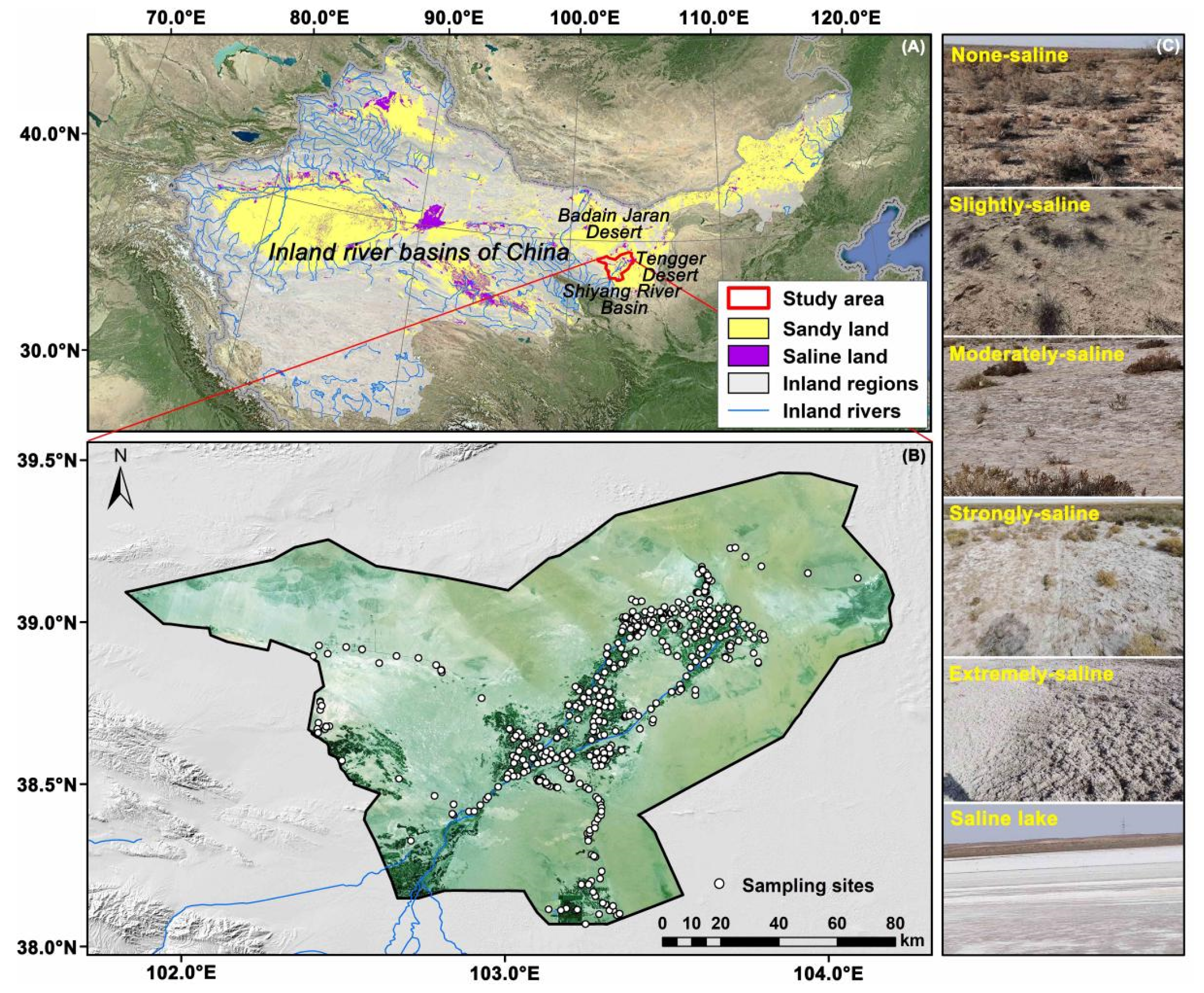
2.1. Study Area
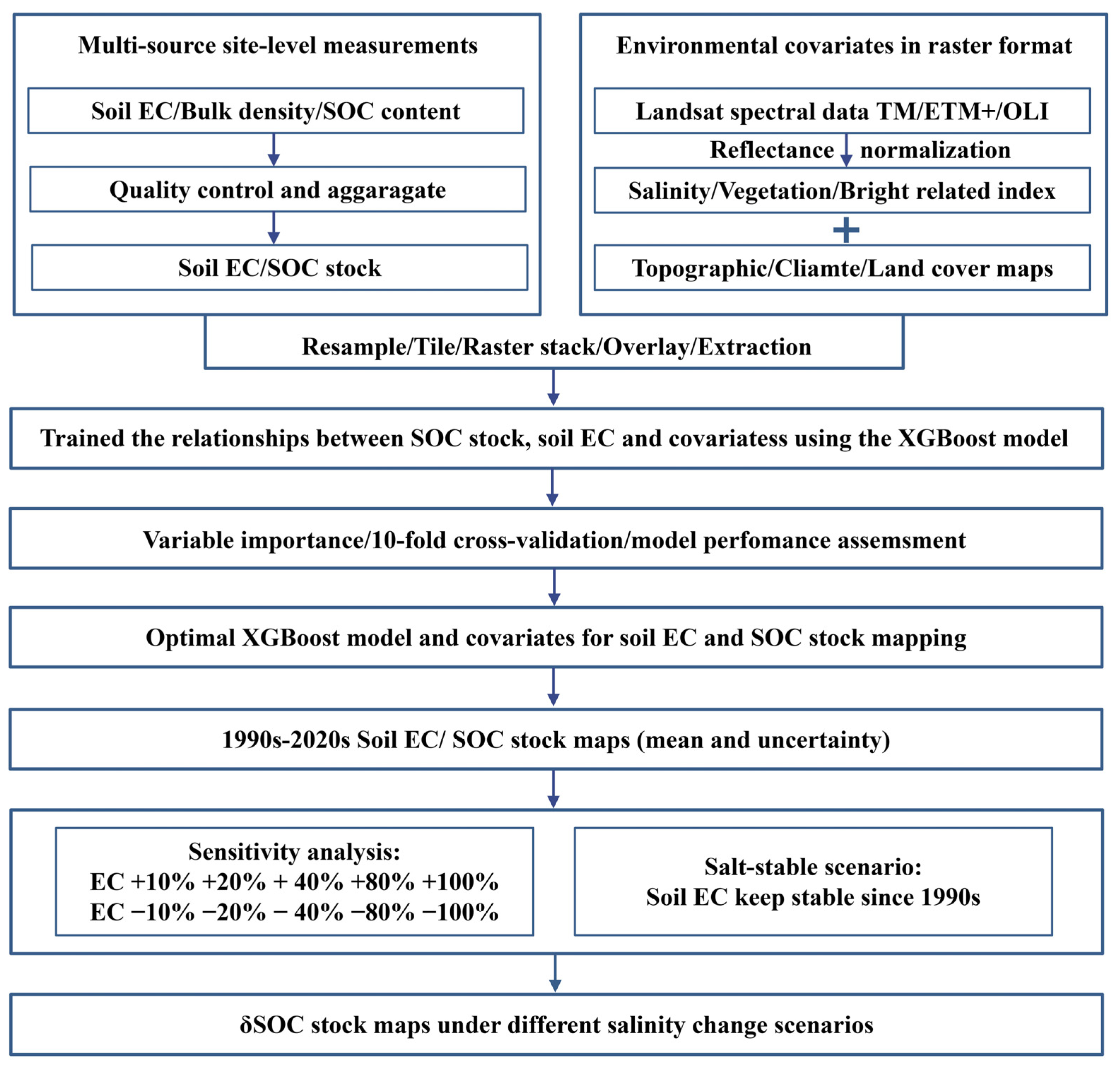
2.2. Methods
2.2.1. Site-Level Soil Measurements
2.2.2. Environmental Covariates
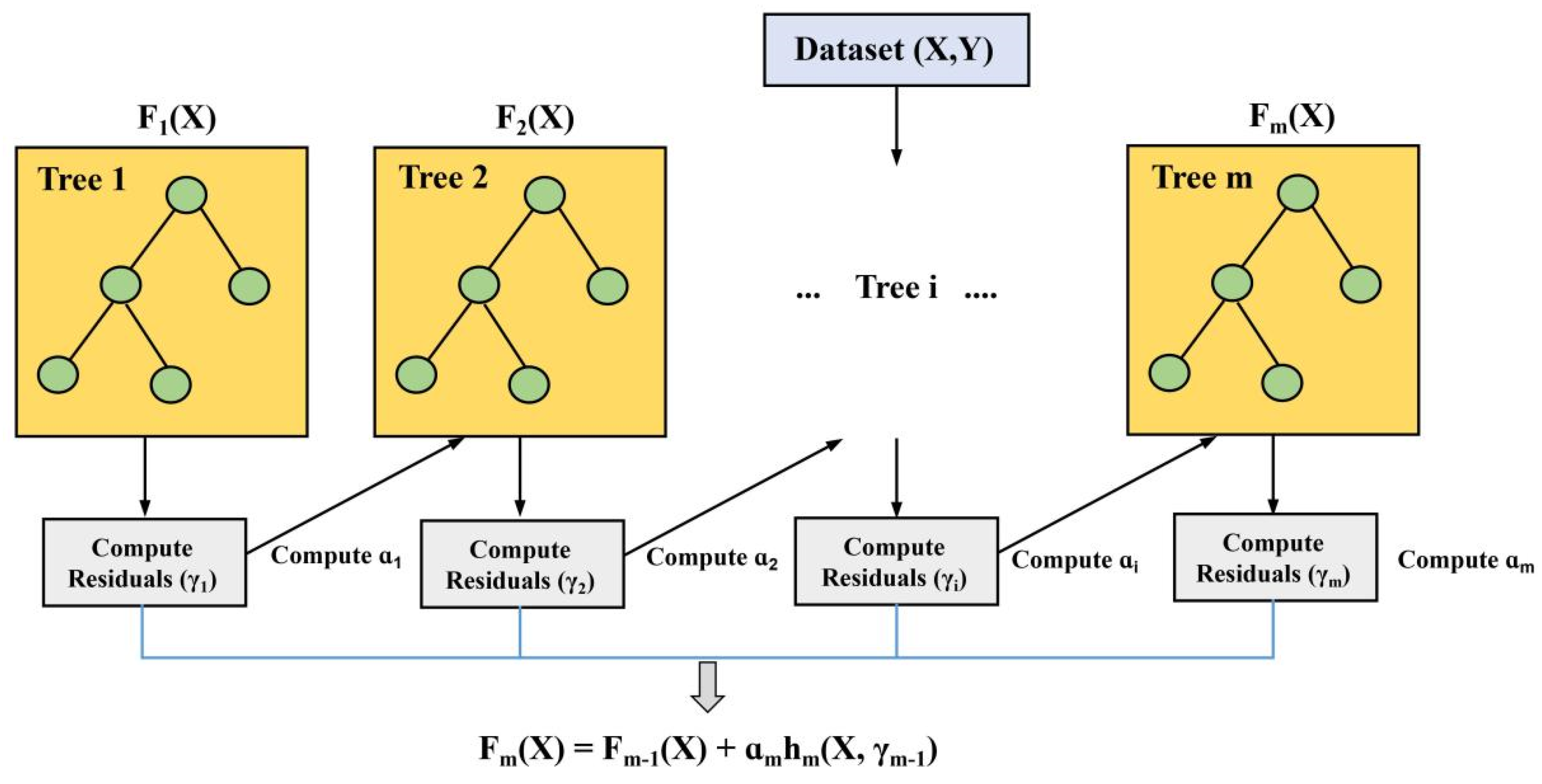
2.2.3. The XGBoost Model
2.2.4. Soil EC and SOC Stock Prediction
2.2.5. Quantification of the Salinity Effect on SOC
3. Results
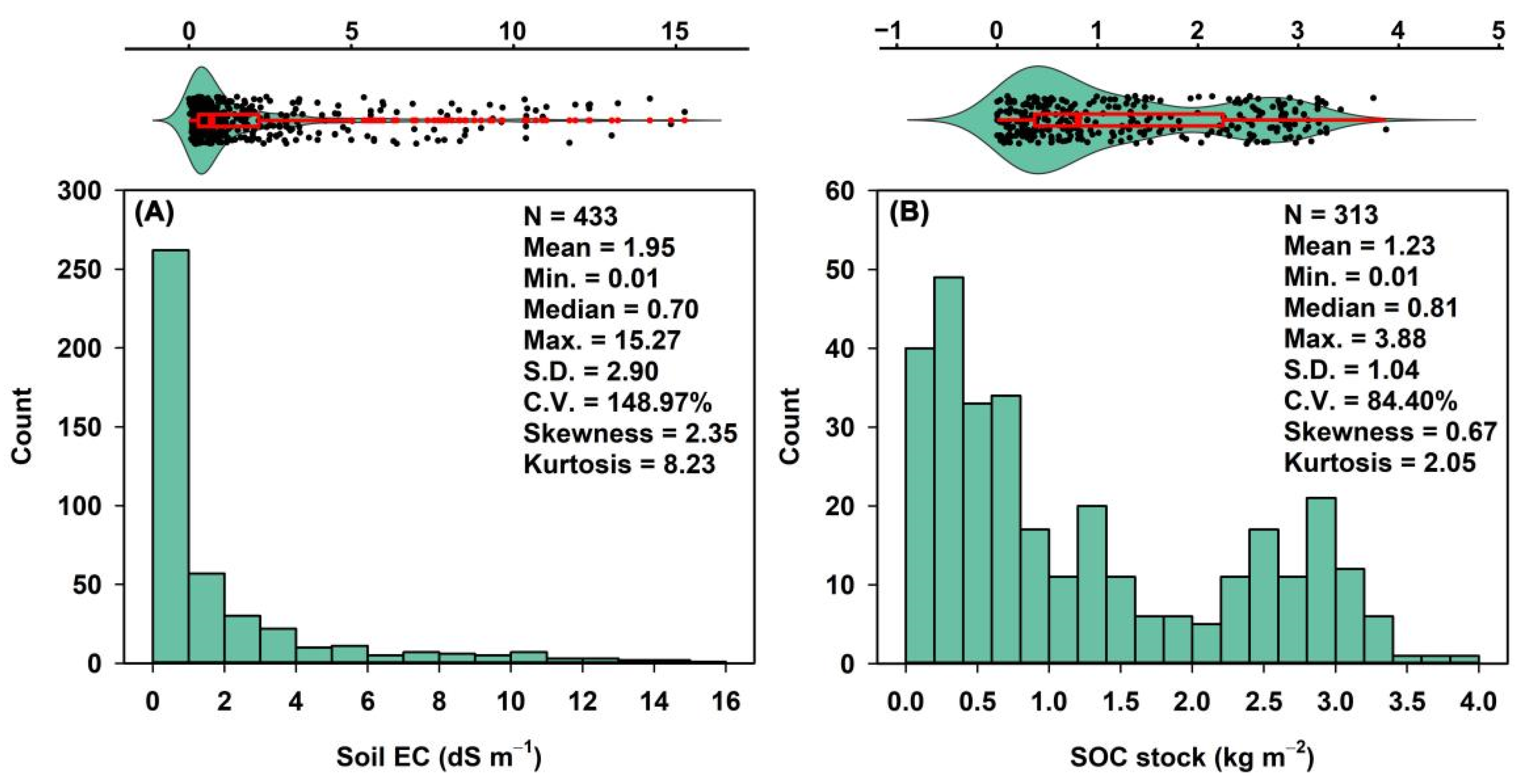
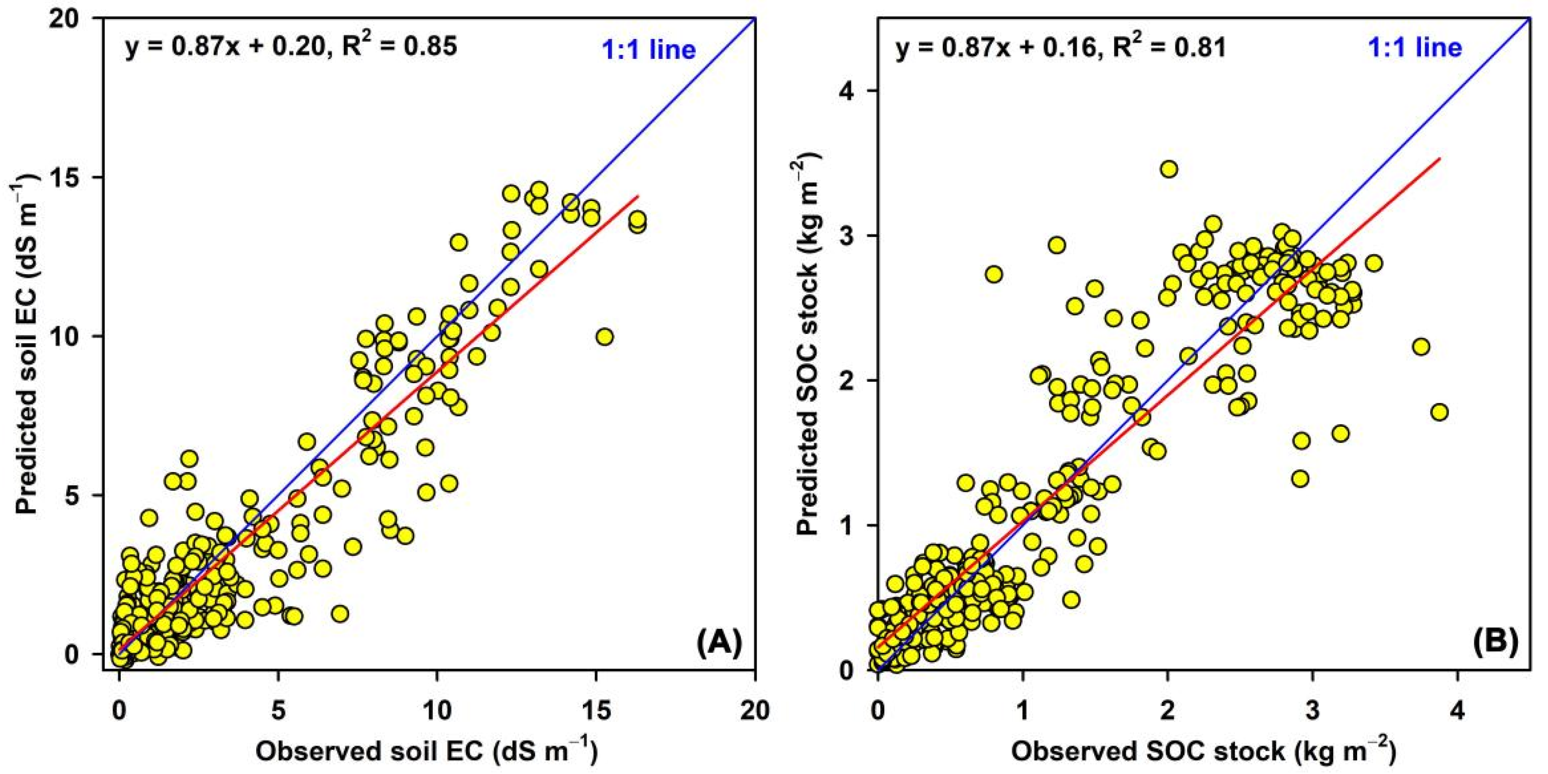
3.1. Soil Salinity and SOC Stock Modeling
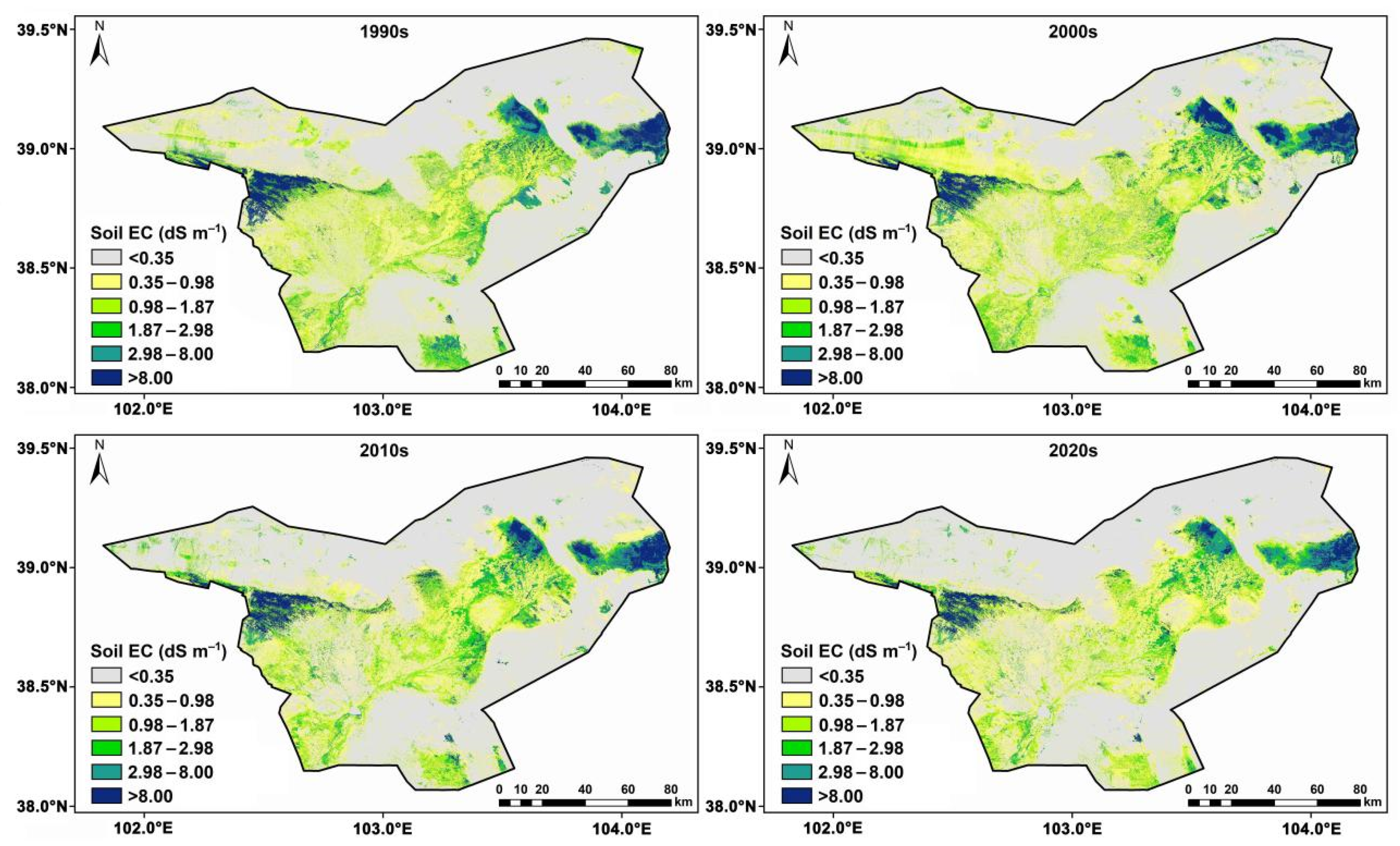
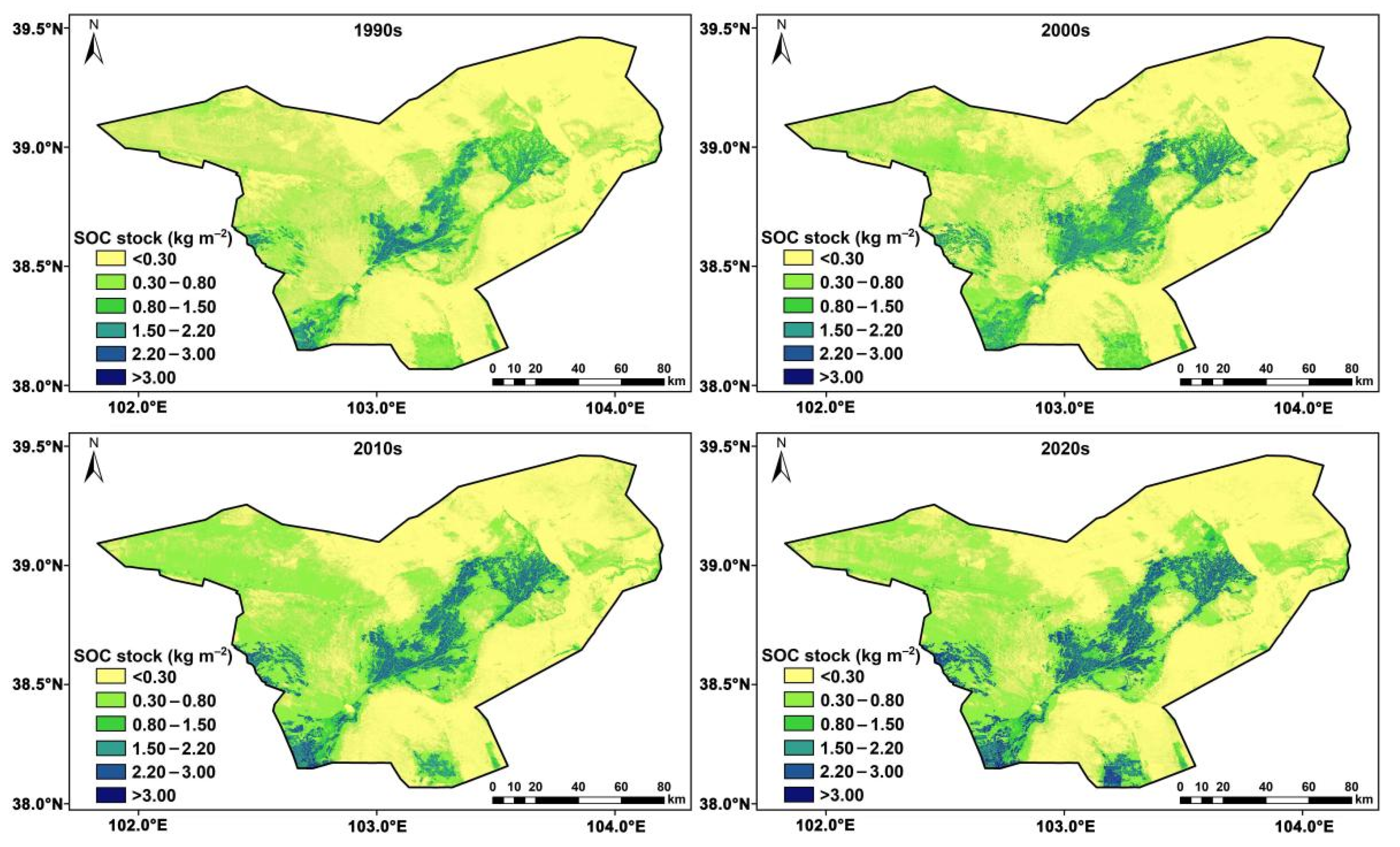
3.2. Spatio-Temporal Patterns of Soil Salinity and SOC Stock
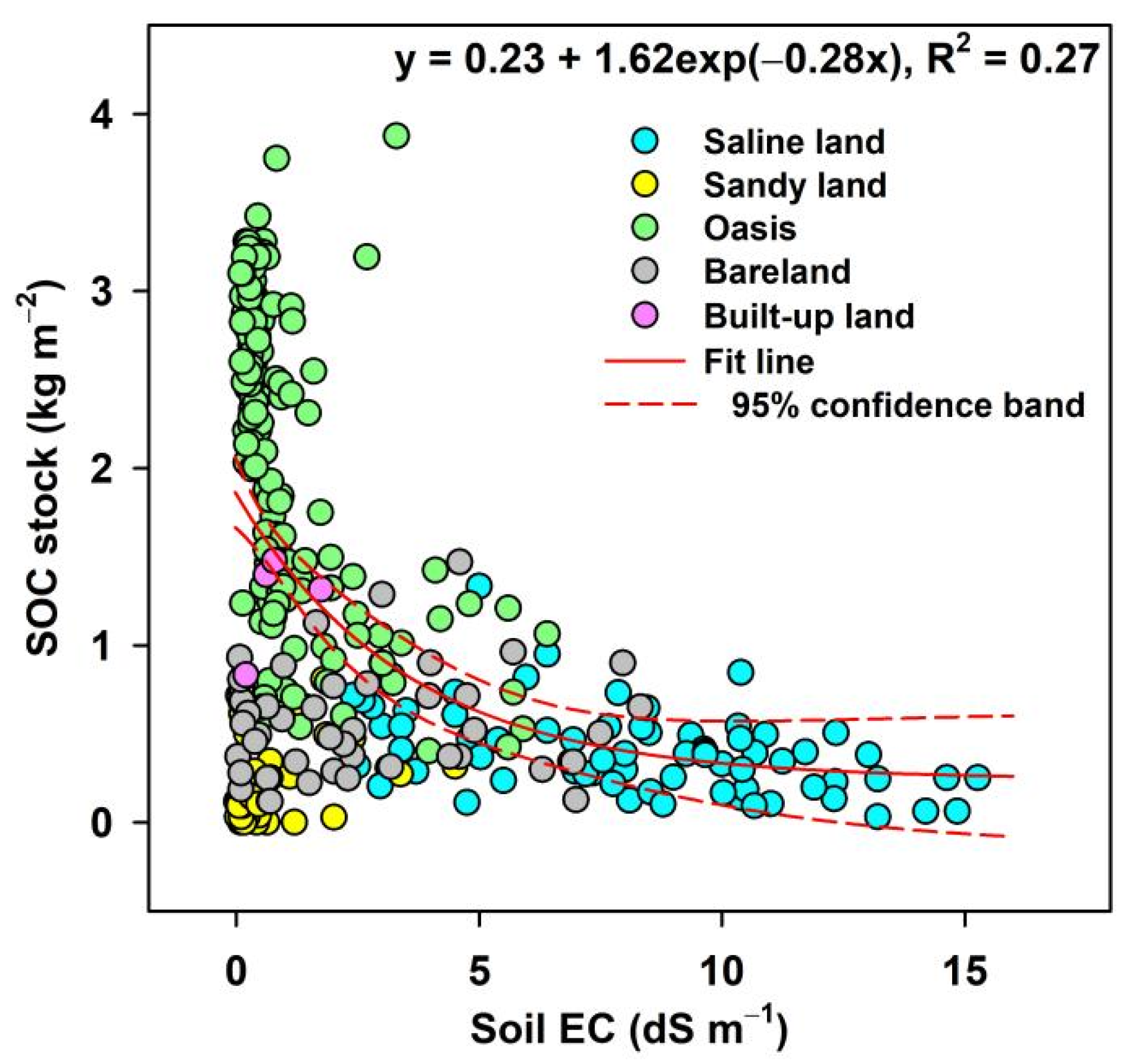
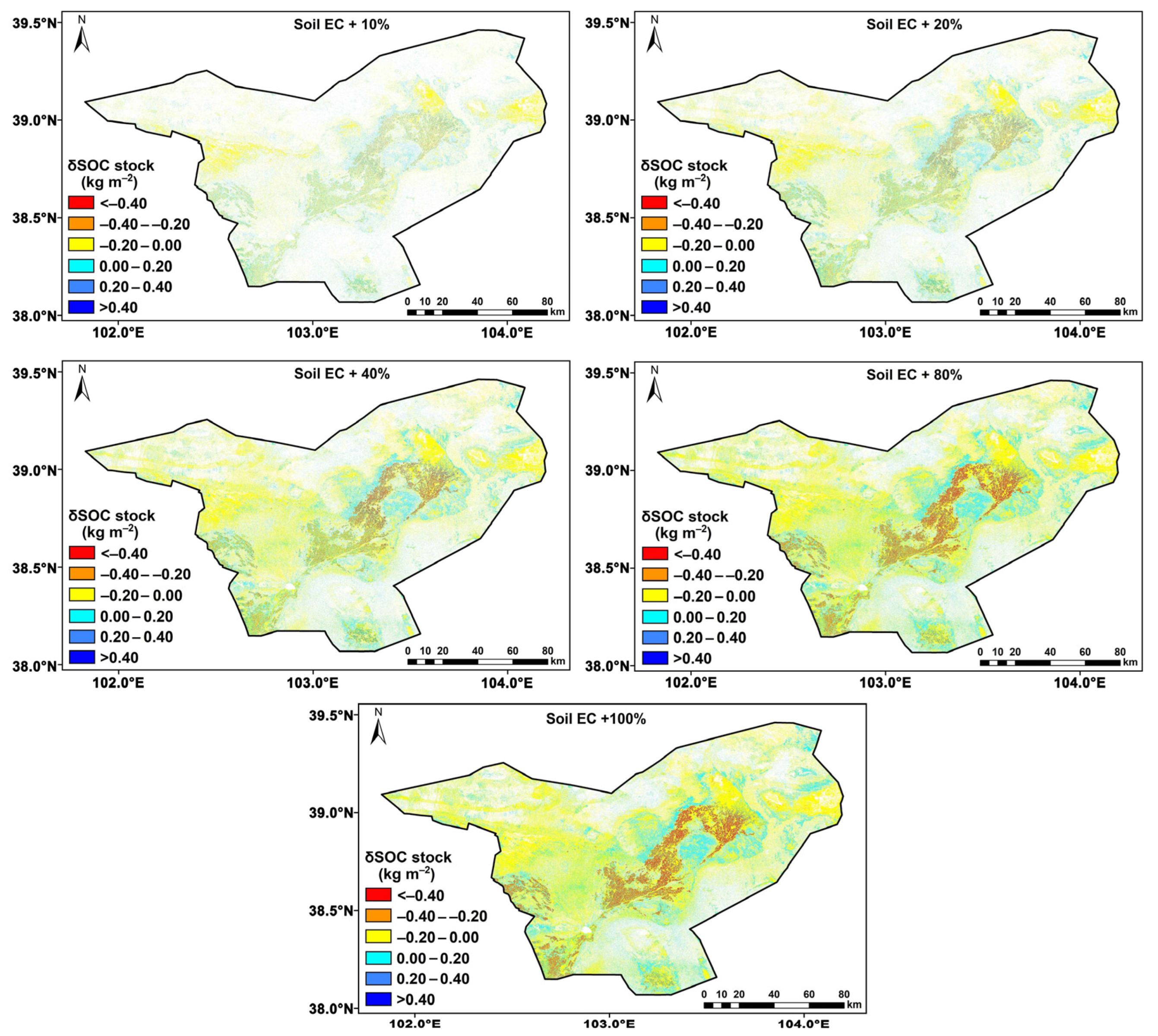
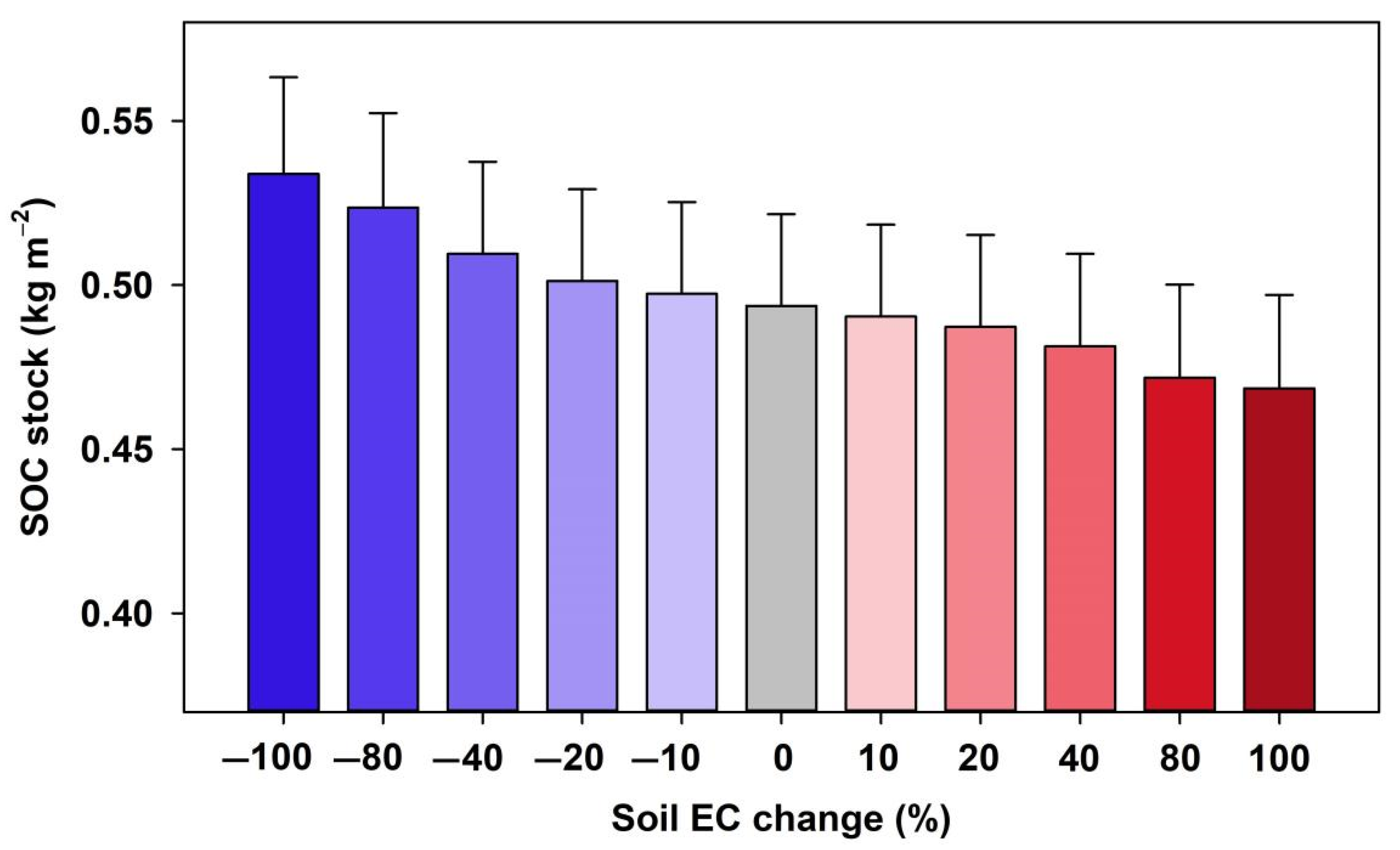
3.3. Effects of Salinity on SOC Stock
4. Discussion
4.1. The Efficiency of the XGBoost Models in Predicting Soil Salinity and SOC Stock
4.2. Spatial Patterns of Soil Salinity and SOC Stock
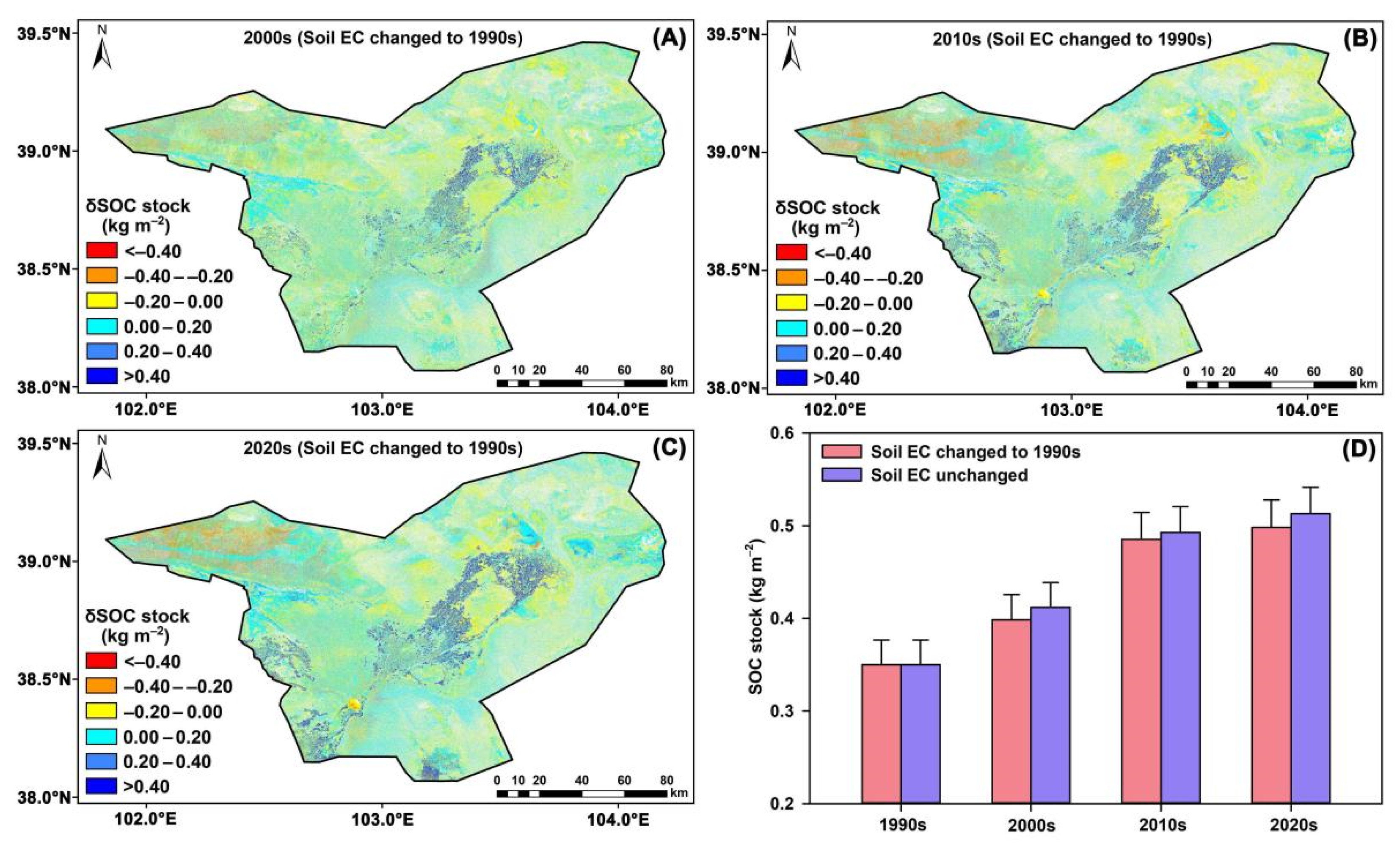
4.3. Temporal Dynamics of Salinity and SOC Stock
4.4. Effects of Salinity on SOC Stock
4.5. Uncertainties and Limitations
5. Conclusions
Supplementary Materials
Author Contributions
Funding
Data Availability Statement
Acknowledgments
Conflicts of Interest
References
- Batjes, N.H. Total carbon and nitrogen in the soils of the world. Eur. J. Soil Sci. 1996, 47, 151–163. [Google Scholar] [CrossRef]
- Stockmann, U.; Adams, M.A.; Crawford, J.W.; Field, D.J.; Henakaarchchi, N.; Jenkins, M.; Minasny, B.; McBratney, A.B.; De Courcelles, V.D.R.; Singh, K.; et al. The knowns, known unknowns and unknowns of sequestration of soil organic carbon. Agric. Ecosyst. Environ. 2013, 164, 80–99. [Google Scholar] [CrossRef]
- Wiesmeier, M.; Urbanski, L.; Hobley, E.; Lang, B.; von Lützow, M.; Marin-Spiotta, E.; van Wesemael, B.; Rabot, E.; Ließ, M.; Garcia-Franco, N.; et al. Soil organic carbon storage as a key function of soils—A review of drivers and indicators at various scales. Geoderma 2019, 333, 149–162. [Google Scholar] [CrossRef]
- Li, H.; Wu, Y.; Chen, J.; Zhao, F.; Wang, F.; Sun, Y.; Zhang, G.; Qiu, L. Responses of soil organic carbon to climate change in the Qilian Mountains and its future projection. J. Hydrol. 2021, 596, 126110. [Google Scholar] [CrossRef]
- Lal, R. Soil carbon sequestration impacts on global climate change and food security. Science 2004, 304, 1623–1627. [Google Scholar] [CrossRef] [Green Version]
- Bangroo, S.A.; Najar, G.R.; Achin, E.; Truong, P.N. Application of predictor variables in spatial quantification of soil organic carbon and total nitrogen using regression kriging in the North Kashmir forest Himalayas. Catena 2020, 193, 104632. [Google Scholar] [CrossRef]
- Li, H.; Wu, Y.; Liu, S.; Xiao, J.; Zhao, W.; Chen, J.; Alexandrov, G.; Cao, Y. Decipher soil organic carbon dynamics and driving forces across China using machine learning. Glob. Chang. Biol. 2022, 28, 3394–3410. [Google Scholar] [CrossRef]
- Scharlemann, J.P.W.; Tanner, E.V.J.; Hiederer, R.; Kapos, V. Global soil carbon: Understanding and managing the largest terrestrial carbon pool. Carbon Manag. 2014, 5, 81–91. [Google Scholar] [CrossRef]
- Lozano-García, B.; Parras-Alcántara, L.; Brevik, E.C. Impact of topographic aspect and vegetation (native and reforested areas) on soil organic carbon and nitrogen budgets in Mediterranean natural areas. Sci. Total Environ. 2016, 544, 963–970. [Google Scholar] [CrossRef]
- Huang, J.; Hartemink, A.E.; Zhang, Y. Climate and land-use change effects on soil carbon stocks over 150 Years in Wisconsin, USA. Remote Sens. 2019, 11, 1504. [Google Scholar] [CrossRef] [Green Version]
- Chen, S.; Arrouays, D.; Angers, D.A.; Chenu, C.; Barré, P.; Martin, M.P.; Saby, N.P.A.; Walter, C. National estimation of soil organic carbon storage potential for arable soils: A data-driven approach coupled with carbon-landscape zones. Sci. Total Environ. 2019, 666, 355–367. [Google Scholar] [CrossRef] [PubMed]
- Setia, R.; Gottschalk, P.; Smith, P.; Marschner, P.; Baldock, J.; Setia, D.; Smith, J. Soil salinity decreases global soil organic carbon stocks. Sci. Total Environ. 2013, 465, 267–272. [Google Scholar] [CrossRef]
- Bhardwaj, A.K.; Mishra, V.K.; Singh, A.K.; Arora, S.; Srivastava, S.; Singh, Y.P.; Sharma, D.K. Soil salinity and land use-land cover interactions with soil carbon in a salt-affected irrigation canal command of Indo-Gangetic plain. Catena 2019, 180, 392–400. [Google Scholar] [CrossRef]
- Wong, V.N.L.; Greene, R.S.B.; Dalal, R.C.; Murphy, B.W. Soil carbon dynamics in saline and sodic soils: A review. Soil Use Manag. 2010, 26, 2–11. [Google Scholar] [CrossRef]
- Hassani, A.; Azapagic, A.; Shokri, N. Global predictions of primary soil salinization under changing climate in the 21st century. Nat. Commun. 2021, 12, 6663. [Google Scholar] [CrossRef]
- Yin, X.; Feng, Q.; Li, Y.; Deo, R.C.; Liu, W.; Zhu, M.; Zheng, X.; Liu, R. An interplay of soil salinization and groundwater degradation threatening coexistence of oasis-desert ecosystems. Sci. Total Environ. 2022, 806, 150599. [Google Scholar] [CrossRef]
- Daliakopoulos, I.N.; Tsanis, I.K.; Koutroulis, A.; Kourgialas, N.N.; Varouchakis, A.E.; Karatzas, G.P.; Ritsema, C.J. The threat of soil salinity: A European scale review. Sci. Total Environ. 2016, 573, 727–739. [Google Scholar] [CrossRef]
- Wang, Y.; Li, Y. Land exploitation resulting in soil salinization in a desert-oasis ecotone. Catena 2013, 100, 50–56. [Google Scholar] [CrossRef]
- Taghizadeh-Mehrjardi, R.; Minasny, B.; Sarmadian, F.; Malone, B.P. Digital mapping of soil salinity in ardakan region, central iran. Geoderma 2014, 213, 15–28. [Google Scholar] [CrossRef]
- Yin, X.; Feng, Q.; Zheng, X.; Zhu, M.; Wu, X.; Guo, Y.; Wu, M.; Li, Y. Spatio-temporal dynamics and eco-hydrological controls of water and salt migration within and among different land uses in an oasis-desert system. Sci. Total Environ. 2021, 772, 145572. [Google Scholar] [CrossRef]
- Huang, J.; Koganti, T.; Santos, F.A.M.; Triantafilis, J. Mapping soil salinity and a fresh-water intrusion in three-dimensions using a quasi-3d joint-inversion of DUALEM-421S and EM34 data. Sci. Total Environ. 2017, 577, 395–404. [Google Scholar] [CrossRef] [PubMed]
- Wang, N.; Peng, J.; Xue, J.; Zhang, X.; Huang, J.; Biswas, A.; He, Y.; Shi, Z. A framework for determining the total salt content of soil profiles using time-series Sentinel-2 images and a random forest-temporal convolution network. Geoderma 2022, 409, 115656. [Google Scholar] [CrossRef]
- Sidike, A.; Zhao, S.; Wen, Y. Estimating soil salinity in Pingluo County of China using QuickBirddata and soil reflectance spectra. Int. J. Appl. Earth Obs. Geoinf. 2014, 26, 156–175. [Google Scholar] [CrossRef]
- Hengl, T.; De Jesus, J.M.; Heuvelink, G.B.M.; Gonzalez, M.R.; Kilibarda, M.; Blagotić, A.; Shangguan, W.; Wright, M.N.; Geng, X.; Bauer-Marschallinger, B.; et al. SoilGrids250m: Global gridded soil information based on machine learning. PLoS ONE 2017, 12, e0169748. [Google Scholar] [CrossRef] [Green Version]
- Ivushkin, K.; Bartholomeus, H.; Bregt, A.K.; Pulatov, A.; Kempen, B.; de Sousa, L. Global mapping of soil salinity change. Remote Sens. Environ. 2019, 231, 111260. [Google Scholar] [CrossRef]
- Wang, J.; Ding, J.; Yu, D.; Teng, D.; He, B.; Chen, X.; Ge, X.; Zhang, Z.; Wang, Y.; Yang, X.; et al. Machine learning-based detection of soil salinity in an arid desert region, Northwest China: A comparison between Landsat-8 OLI and Sentinel-2 MSI. Sci. Total Environ. 2020, 707, 136092. [Google Scholar] [CrossRef]
- Taghizadeh-Mehrjardi, R.; Schmidt, K.; Toomanian, N.; Heung, B.; Behrens, T.; Mosavi, A.; Band, S.S.; Amirian-Chakan, A.; Fathabadi, A.; Scholten, T. Improving the spatial prediction of soil salinity in arid regions using wavelet transformation and support vector regression models. Geoderma 2021, 383, 114793. [Google Scholar] [CrossRef]
- Abbas, A.; Khan, S. Using remote sensing techniques for appraisal of irrigated soil salinity. In Proceedings of the MODSIM 2007 International Congress on Modelling and Simulation, Christchurch, New Zealand, 10–13 December 2007; pp. 2632–2638. [Google Scholar]
- Peng, J.; Biswas, A.; Jiang, Q.; Zhao, R.; Hu, J.; Hu, B.; Shi, Z. Estimating soil salinity from remote sensing and terrain data in southern Xinjiang Province, China. Geoderma 2019, 337, 1309–1319. [Google Scholar] [CrossRef]
- Nabiollahi, K.; Taghizadeh-Mehrjardi, R.; Shahabi, A.; Heung, B.; Amirian-Chakan, A.; Davari, M.; Scholten, T. Assessing agricultural salt-affected land using digital soil mapping and hybridized random forests. Geoderma 2021, 385, 114858. [Google Scholar] [CrossRef]
- Gray, J.M.; Bishop, T.F.A. Change in soil organic carbon stocks under 12 climate change projections over New South Wales, Australia. Soil Sci. Soc. Am. J. 2016, 80, 1296–1307. [Google Scholar] [CrossRef] [Green Version]
- Adhikari, K.; Owens, P.R.; Libohova, Z.; Miller, D.M.; Wills, S.A.; Nemecek, J. Assessing soil organic carbon stock of Wisconsin, USA and its fate under future land use and climate change. Sci. Total Environ. 2019, 667, 833–845. [Google Scholar] [CrossRef] [PubMed]
- Wang, L.; Wang, X.; Wang, D.; Qi, B.; Zheng, S.; Liu, H.; Luo, C.; Li, H.; Meng, L.; Meng, X.; et al. Spatiotemporal changes and driving factors of cultivated soil organic carbon in northern China’s typical agro-pastoral ecotone in the last 30 years. Remote Sens. 2021, 13, 3607. [Google Scholar] [CrossRef]
- Ramcharan, A.; Hengl, T.; Nauman, T.; Brungard, C.; Waltman, S.; Wills, S.; Thompson, J. Soil property and class maps of the conterminous United States at 100-meter spatial resolution. Soil Sci. Soc. Am. J. 2018, 82, 186–201. [Google Scholar] [CrossRef] [Green Version]
- Gautam, S.; Mishra, U.; Scown, C.D.; Wills, S.A.; Adhikari, K.; Drewniak, B.A. Continental United States may lose 1.8 petagrams of soil organic carbon under climate change by 2100. Glob. Ecol. Biogeogr. 2022, 31, 1147–1160. [Google Scholar] [CrossRef]
- Wadoux, A.M.J.C.; Minasny, B.; McBratney, A.B. Machine learning for digital soil mapping: Applications, challenges and suggested solutions. Earth-Sci. Rev. 2020, 210, 103359. [Google Scholar] [CrossRef]
- Chen, S.; Arrouays, D.; Leatitia Mulder, V.; Poggio, L.; Minasny, B.; Roudier, P.; Libohova, Z.; Lagacherie, P.; Shi, Z.; Hannam, J.; et al. Digital mapping of GlobalSoilMap soil properties at a broad scale: A review. Geoderma 2022, 409, 115567. [Google Scholar] [CrossRef]
- Perri, S.; Suweis, S.; Holmes, A.; Marpu, P.R.; Entekhabi, D.; Molini, A. River basin salinization as a form of aridity. Proc. Natl. Acad. Sci. USA 2020, 117, 17635–17642. [Google Scholar] [CrossRef]
- Huang, J.; Hartemink, A.E. Soil and environmental issues in sandy soils. Earth-Sci. Rev. 2020, 208, 103295. [Google Scholar] [CrossRef]
- Rath, K.M.; Murphy, D.N.; Rousk, J. The microbial community size, structure, and process rates along natural gradients of soil salinity. Soil Biol. Biochem. 2019, 138, 107607. [Google Scholar] [CrossRef]
- Rath, K.M.; Fierer, N.; Murphy, D.V.; Rousk, J. Linking bacterial community composition to soil salinity along environmental gradients. ISME J. 2019, 13, 836–846. [Google Scholar] [CrossRef] [Green Version]
- IUSS Working Group WRB. World Reference Base for Soil Resources 2014, Update 2015 International Soil Classification System for Naming Soils and Creating Legends for Soil Maps; World Soil Resources Reports, No. 106; FAO: Rome, Italy, 2015. [Google Scholar]
- Chen, L.H.; Qu, Y.G.; Chen, H.S.; Li, F.X. Water and Land Resources and Their Rational Development and Utilization in the Hexi Region; Science Press: Beijing, China, 1992. (In Chinese) [Google Scholar]
- Feng, Q.; Yang, L.; Deo, R.C.; Aghakouchak, A.; Adamowski, J.F.; Stone, R.; Yin, Z.; Liu, W.; Si, J.; Wen, X.; et al. Domino effect of climate change over two millennia in ancient China’s Hexi Corridor. Nat. Sustain. 2019, 2, 957–961. [Google Scholar] [CrossRef]
- Li, Y.; Liu, W.; Feng, Q.; Zhu, M.; Yang, L.; Zhang, J. Effects of land use and land cover change on soil organic carbon storage in the Hexi regions, Northwest China. J. Environ. Manage. 2022, 312, 114911. [Google Scholar] [CrossRef]
- Qi, S.; Liu, W.; Shu, H.; Liu, F.; Ma, J. Soil NO3− storage from oasis development in deserts: Implications for the prevention and control of groundwater pollution. Hydrol. Process. 2020, 34, 3941–3954. [Google Scholar] [CrossRef]
- McBratney, A.B.; Mendonça Santos, M.L.; Minasny, B. On digital soil mapping. Geoderma 2003, 117, 3–52. [Google Scholar] [CrossRef]
- Minasny, B.; McBratney, A.B.; Mendonça-Santos, M.L.; Odeh, I.O.A.; Guyon, B. Prediction and digital mapping of soil carbon storage in the lower Namoi Valley. Aust. J. Soil Res. 2006, 44, 233–244. [Google Scholar] [CrossRef]
- Minasny, B.; McBratney, A.B. Digital soil mapping: A brief history and some lessons. Geoderma 2016, 264, 301–311. [Google Scholar] [CrossRef]
- Sommers, L.E.; Nelson, D.W. Determination of total phosphorus in soils: A rapid perchloric acid digestion procedure. Soil Sci. Soc. Am. J. 1972, 36, 902–904. [Google Scholar] [CrossRef]
- Chen, L.J.; Feng, Q.; Cheng, A.F. Spatial distribution of soil water and salt contents and reasons of saline soils’ development in the Minqin oasis. J. Arid. Land Resour. Environ. 2013, 27, 99–105. (In Chinese) [Google Scholar]
- Li, H.Y.; Feng, Q.; Chen, L.J.; Zhao, Y.; Zhu, M. Spatial distribution characteristics of topsoil salinity in the Minqin oasis, Northwest China. J. Arid. Land Resour. Environ. 2017, 31, 136–141. (In Chinese) [Google Scholar]
- McCune, B.; Keon, D. Equations for potential annual direct incident radiation and heat load. J. Veg. Sci. 2002, 13, 603–606. [Google Scholar] [CrossRef]
- Peng, S.; Ding, Y.; Liu, W.; Li, Z. 1 km monthly temperature and precipitation dataset for China from 1901 to 2017. Earth Syst. Sci. Data 2019, 11, 1931–1946. [Google Scholar] [CrossRef] [Green Version]
- Lai, L.; Huang, X.; Yang, H.; Chuai, X.; Zhang, M.; Zhong, T.; Chen, Z.; Chen, Y.; Wang, X.; Thompson, J.R. Carbon emissions from land-use change and management in China between 1990 and 2010. Sci. Adv. 2016, 2, e1601063. [Google Scholar] [CrossRef] [Green Version]
- Roy, D.P.; Zhang, H.K.; Ju, J.; Gomez-Dans, J.L.; Lewis, P.E.; Schaaf, C.B.; Sun, Q.; Li, J.; Huang, H.; Kovalskyy, V. A general method to normalize Landsat reflectance data to nadir BRDF adjusted reflectance. Remote Sens. Environ. 2016, 176, 255–271. [Google Scholar] [CrossRef] [Green Version]
- Chen, T.Q.; Guestrin, G. XGBoost: A scalable tree boosting system. In Proceedings of the 22nd ACM SIGKDD International Conference on Knowledge Discovery and Data Mining, San Francisco, CA, USA, 13–17 August 2016; pp. 785–794. [Google Scholar] [CrossRef] [Green Version]
- Chen, S.; Liang, Z.; Webster, R.; Zhang, G.; Zhou, Y.; Teng, H.; Hu, B.; Arrouays, D.; Shi, Z. A high-resolution map of soil pH in China made by hybrid modelling of sparse soil data and environmental covariates and its implications for pollution. Sci. Total Environ. 2019, 655, 273–283. [Google Scholar] [CrossRef]
- Liang, Z.; Chen, S.; Yang, Y.; Zhou, Y.; Shi, Z. High-resolution three-dimensional mapping of soil organic carbon in China: Effects of SoilGrids products on national modeling. Sci. Total Environ. 2019, 685, 480–489. [Google Scholar] [CrossRef]
- Zhu, M.; Feng, Q.; Zhang, M.; Liu, W.; Deo, R.C.; Zhang, C.; Yang, L. Soil organic carbon in semiarid alpine regions: The spatial distribution, stock estimation, and environmental controls. J. Soils Sediments 2019, 19, 3427–3441. [Google Scholar] [CrossRef]
- R Development Core Team. R: A Language and Environment for Statistical Computing; R Foundation for Statistical Computing: Vienna, Austria, 2021. [Google Scholar]
- Zepp, S.; Heiden, U.; Bachmann, M.; Wiesmeier, M.; Steininger, M.; van Wesemael, B. Estimation of soil organic carbon contents in croplands of bavaria from SCMaP soil reflectance composites. Remote Sens. 2021, 13, 3141. [Google Scholar] [CrossRef]
- Li, B. A study on the Zhuye Lake and its historical evolution. Acta Geogr. Sin. 1993, 48, 5560, (In Chinese with English Abstract). [Google Scholar]
- Schoeneberger, P.J.; Wysocki, D.A.; Benham, E.C.; Broderson, W.D. Field Book for Describing and Sampling Soils. Version 2.0; USDA: Washington, DC, USA, 2002.
- Liu, M.; Jiang, Y.; Xu, X.; Huang, Q.; Huo, Z.; Huang, G. Long-term groundwater dynamics affected by intense agricultural activities in oasis areas of arid inland river basins, Northwest China. Agric. Water Manag. 2018, 203, 37–52. [Google Scholar] [CrossRef]
- Hassani, A.; Azapagic, A.; Shokri, N. Predicting long-term dynamics of soil salinity and sodicity on a global scale. Proc. Natl. Acad. Sci. USA 2020, 117, 33017–33027. [Google Scholar] [CrossRef]
- Wang, Y.; Jiang, J.; Niu, Z.; Li, Y.; Li, C.; Feng, W. Responses of soil organic and inorganic carbon vary at different soil depths after long-term agricultural cultivation in Northwest China. Land Degrad. Dev. 2019, 30, 1229–1242. [Google Scholar] [CrossRef]
- Dong, Y.; Chen, R.; Petropoulos, E.; Yu, B.; Zhang, J.; Lin, X.; Gao, M.; Feng, Y. Interactive effects of salinity and SOM on the ecoenzymatic activities across coastal soils subjected to a saline gradient. Geoderma 2022, 406, 115519. [Google Scholar] [CrossRef]
- Yuan, B.C.; Li, Z.Z.; Liu, H.; Gao, M.; Zhang, Y.Y. Microbial biomass and activity in salt affected soils under arid conditions. Appl. Soil Ecol. 2007, 35, 319–328. [Google Scholar] [CrossRef]
- Singh, K. Microbial and enzyme activities of saline and sodic soils. Land Degrad. Dev. 2016, 27, 706–718. [Google Scholar] [CrossRef]
- Rath, K.M.; Rousk, J. Salt effects on the soil microbial decomposer community and their role in organic carbon cycling: A review. Soil Biol. Biochem. 2015, 81, 108–123. [Google Scholar] [CrossRef]
- Liang, C.; Schimel, J.P.; Jastrow, J.D. The importance of anabolism in microbial control over soil carbon storage. Nat Microbiol. 2017, 2, 17105. [Google Scholar] [CrossRef]
- Zhu, X.; Jackson, R.D.; DeLucia, E.H.; Tiedje, J.M.; Liang, C. The soil microbial carbon pump: From conceptual insights to empirical assessments. Glob. Chang. Biol. 2020, 26, 6032–6039. [Google Scholar] [CrossRef]
- Yang, L.; He, X.; Shen, F.; Zhou, C.; Zhu, A.X.; Gao, B.; Chen, Z.; Li, M. Improving prediction of soil organic carbon content in croplands using phenological parameters extracted from NDVI time series data. Soil Tillage Res. 2020, 196, 104465. [Google Scholar] [CrossRef]
- Hu, B.; Zhou, Q.; He, C.; Duan, L.; Li, W.; Zhang, G.; Ji, W.; Peng, J.; Xie, H. Spatial variability and potential controls of soil organic matter in the Eastern Dongting Lake Plain in southern China. J. Soils Sediments 2021, 21, 2791–2804. [Google Scholar] [CrossRef]


| Variable | Statistics | Minimum | 1st Quartile | Median | Mean | 3rd Quartile | Maximum | Standard Deviation |
|---|---|---|---|---|---|---|---|---|
| Soil EC (dS m−1) | MAE | 0.57 | 0.58 | 0.60 | 0.60 | 0.61 | 0.62 | 0.02 |
| RMSE | 1.28 | 1.37 | 1.41 | 1.41 | 1.45 | 1.51 | 0.06 | |
| R2 | 0.81 | 0.84 | 0.85 | 0.85 | 0.85 | 0.88 | 0.02 | |
| LCCC | 0.89 | 0.91 | 0.91 | 0.91 | 0.92 | 0.93 | 0.01 | |
| SOC stock (kg m−2) | MAE | 0.30 | 0.31 | 0.32 | 0.32 | 0.32 | 0.33 | 0.01 |
| RMSE | 0.45 | 0.45 | 0.46 | 0.46 | 0.47 | 0.49 | 0.01 | |
| R2 | 0.79 | 0.80 | 0.81 | 0.81 | 0.81 | 0.82 | 0.01 | |
| LCCC | 0.89 | 0.90 | 0.90 | 0.90 | 0.90 | 0.90 | 0.00 |
| Variable | Type | Periods | |||
|---|---|---|---|---|---|
| 1990s | 2000s | 2010s | 2020s | ||
| Soil EC (dS m–1) | Bare land | 0.63 ± 0.13 | 0.65 ± 0.12 | 0.61 ± 0.11 | 0.48 ± 0.28 |
| Built-up land | 1.19 ± 0.14 | 1.14 ± 0.16 | 1.12 ± 0.15 | 1.29 ± 0.48 | |
| Oasis | 1.18 ± 0.14 | 1.12 ± 0.16 | 1.03 ± 0.13 | 0.96 ± 0.24 | |
| Saline land | 4.78 ± 0.30 | 4.37 ± 0.30 | 4.52 ± 0.31 | 3.38 ± 0.91 | |
| Sandy land | 0.54 ± 0.09 | 0.59 ± 0.10 | 0.58 ± 0.09 | 0.49 ± 0.34 | |
| Area-weighted mean | 1.17 ± 0.14 | 1.13 ± 0.14 | 1.07 ± 0.13 | 0.85 ± 0.12 | |
| SOC stock (kg m–2) | Bare land | 0.29 ± 0.06 | 0.35 ± 0.07 | 0.40 ± 0.07 | 0.37 ± 0.08 |
| Built-up land | 1.28 ± 0.12 | 1.33 ± 0.14 | 1.49 ± 0.16 | 1.40 ± 0.20 | |
| Oasis | 1.28 ± 0.15 | 1.54 ± 0.15 | 1.69 ± 0.18 | 1.88 ± 0.21 | |
| Saline land | 0.38 ± 0.06 | 0.43 ± 0.08 | 0.47 ± 0.08 | 0.51 ± 0.09 | |
| Sandy land | 0.17 ± 0.04 | 0.19 ± 0.05 | 0.23 ± 0.05 | 0.22 ± 0.05 | |
| Area-weighted mean | 0.35 ± 0.03 | 0.41 ± 0.03 | 0.49 ± 0.03 | 0.51 ± 0.03 | |
| Soil EC Change | δSOC Stock (g m−2) | ||||
|---|---|---|---|---|---|
| Bare Land | Build-Up Land | Oasis | Saline Land | Sandy Land | |
| −100% | 23.20 ± 11.35 | 113.99 ± 44.95 | 139.83 ± 48.02 | 71.52 ± 19.11 | 17.89 ± 8.13 |
| −80% | 15.84 ± 10.17 | 96.21 ± 42.32 | 116.88 ± 44.86 | 48.06 ± 17.89 | 12.13 ± 6.92 |
| −40% | 6.69 ± 7.66 | 56.60 ± 37.74 | 67.49 ± 40.60 | 30.58 ± 13.50 | 4.89 ± 4.77 |
| −20% | 3.08 ± 5.47 | 27.02 ± 29.85 | 34.10 ± 32.50 | 13.69 ± 8.36 | 2.22 ± 2.98 |
| −10% | 1.48 ± 3.60 | 13.24 ± 20.26 | 16.76 ± 22.18 | 6.16 ± 5.17 | 1.05 ± 1.92 |
| +10% | −1.33 ± 3.47 | −12.74 ± 19.81 | −16.24 ± 22.03 | −4.66 ± 4.54 | −0.89 ± 1.79 |
| +20% | −2.55 ± 5.12 | −25.77 ± 29.59 | −32.47 ± 32.79 | −8.71 ± 6.73 | −1.69 ± 2.66 |
| +40% | −4.72 ± 6.92 | −52.96 ± 39.70 | −65.28 ± 43.61 | −15.07 ± 9.30 | −2.98 ± 3.87 |
| +80% | −8.22 ± 8.97 | −95.54 ± 47.69 | −120.39 ± 52.42 | −24.68 ± 12.40 | −4.70 ± 5.35 |
| +100% | −9.59 ± 9.53 | −107.82 ± 48.53 | −137.78 ± 53.55 | −28.44 ± 13.30 | −5.31 ± 5.83 |
| Type | δSOC Stock (g m−2) | ||
|---|---|---|---|
| 2000s | 2010s | 2020s | |
| Bare land | 6.29 ± 18.47 | −7.38 ± 22.29 | −3.43 ± 24.11 |
| Built-up land | 53.85 ± 40.29 | 58.70 ± 45.02 | 47.20 ± 46.86 |
| Oasis | 76.32 ± 46.48 | 73.84 ± 50.11 | 94.24 ± 54.18 |
| Saline land | 8.77 ± 17.00 | 7.72 ± 18.63 | 23.34 ± 21.55 |
| Sandy land | 6.71 ± 14.21 | 1.37 ± 13.20 | 6.03 ± 12.99 |
Publisher’s Note: MDPI stays neutral with regard to jurisdictional claims in published maps and institutional affiliations. |
© 2022 by the authors. Licensee MDPI, Basel, Switzerland. This article is an open access article distributed under the terms and conditions of the Creative Commons Attribution (CC BY) license (https://creativecommons.org/licenses/by/4.0/).
Share and Cite
Zhang, W.; Zhang, W.; Liu, Y.; Zhang, J.; Yang, L.; Wang, Z.; Mao, Z.; Qi, S.; Zhang, C.; Yin, Z. The Role of Soil Salinization in Shaping the Spatio-Temporal Patterns of Soil Organic Carbon Stock. Remote Sens. 2022, 14, 3204. https://doi.org/10.3390/rs14133204
Zhang W, Zhang W, Liu Y, Zhang J, Yang L, Wang Z, Mao Z, Qi S, Zhang C, Yin Z. The Role of Soil Salinization in Shaping the Spatio-Temporal Patterns of Soil Organic Carbon Stock. Remote Sensing. 2022; 14(13):3204. https://doi.org/10.3390/rs14133204
Chicago/Turabian StyleZhang, Wenli, Wei Zhang, Yubing Liu, Jutao Zhang, Linshan Yang, Zengru Wang, Zhongchao Mao, Shi Qi, Chengqi Zhang, and Zhenliang Yin. 2022. "The Role of Soil Salinization in Shaping the Spatio-Temporal Patterns of Soil Organic Carbon Stock" Remote Sensing 14, no. 13: 3204. https://doi.org/10.3390/rs14133204
APA StyleZhang, W., Zhang, W., Liu, Y., Zhang, J., Yang, L., Wang, Z., Mao, Z., Qi, S., Zhang, C., & Yin, Z. (2022). The Role of Soil Salinization in Shaping the Spatio-Temporal Patterns of Soil Organic Carbon Stock. Remote Sensing, 14(13), 3204. https://doi.org/10.3390/rs14133204