Article

Retrieval of Soil Moisture Content Based on Multisatellite Dual-Frequency Combination Multipath Errors

College of Geographic Information and Tourism, Chuzhou University, Chuzhou 239000, China
*
Author to whom correspondence should be addressed.
Remote Sens. 2022, 14(13), 3193; https://doi.org/10.3390/rs14133193
Submission received: 28 April 2022 / Revised: 30 June 2022 / Accepted: 1 July 2022 / Published: 3 July 2022
(This article belongs to the Special Issue GNSS, Space Weather and TEC Special Features)

Abstract

:
Global navigation satellite system interferometric reflectometry (GNSS-IR) is a new type of microwave remote sensing technology that can measure soil moisture content (SMC). GNSS-IR soil moisture retrieval methods based on the satellite signal-to-noise ratio (SNR) and triple-frequency signal combination have the following shortcomings: SNR does not always exist in the original GNSS file, and the number of triple-frequency signal observation satellites is small, resulting in GNSS-IR soil moisture observation time resolution being low. Based on the above problems, in this study, we constructed a soil moisture inversion method based on multisatellite dual-frequency combined multipath error is proposed: the multipath error calculation model of dual-frequency carrier phase (L4 Ionosphere Free, L4_IF) and dual-frequency pseudorange (DFP) without ionospheric effect is constructed. We selected the data of the five epochs before and after the time point of the effective satellite period to construct the multipath error model and error equation, and we solved the delay phase for soil moisture retrieval. We verified the method using Plate Boundary Observatory (PBO) P041 site data. The results showed that the Pearson correlation coefficients (R) of L4_IF and DFP methods at P041 station are 0.97 and 0.91, respectively. To better verify the results’ reliability and the proposed method’s effectiveness, the soil moisture data of the MFLE station about 210 m away from P041 station are used as the verification data in this paper. The results showed that the delay phase solved by multipath error and soil moisture strongly correlate. Pearson correlation coefficients (R) of L4_IF and DFP methods at MFLE station are 0.93 and 0.86, respectively. In order to improve the inversion accuracy of GNSS-IR soil moisture, this paper constructs the prediction model of soil moisture by using the linear regression (ULR), back propagation neural network (BPNN) and radial basis function neural network (RBFNN), and evaluates the accuracy of each model. The results showed that the soil moisture retrieval method based on multisatellite dual-frequency combined multipath error can replace the traditional retrieval method and effectively improve the time resolution of GNSS-IR soil moisture estimation. To perform highly dynamic monitoring of soil moisture, higher retrieval accuracy can only be obtained with a small epoch multipath error.

Graphical Abstract

1. Introduction

Soil moisture content (SMC) is the physical quantity that characterizes the degree of soil wetting and drying. As an indispensable environmental factor on the surface, SMC plays an active role in weather forecast, climate research, slope stability prediction, and accurate prediction of flood disasters [1,2,3,4]. Global Navigation Satellite System interferometric reflection (GNSS-IR) is a new microwave remote sensing technology that mainly uses the interference effect generated by the direct and surface reflection signals obtained at the GNSS receiver to invert the surface parameters according to the characteristics of the interference signals [5,6,7,8,9].
In recent years, many scholars have made remarkable achievements in soil moisture retrieval using GNSS-IR technology. Larson et al. observed that the ground-reflected signal captured by a geodetic-quality Global Positioning System (GPS) antenna is sensitive to soil moisture, so the GPS signals can be used to sense soil moisture. They first proposed using GPS SNR retrieval of soil moisture, confirming the feasibility of SNR data retrieval [10,11,12]. Zhang et al. used Bei Dou Navigation Satellite System (BDS) and GPS SNR to invert volumetric soil moisture (VSM) changes and wheat growth, and compared the results with the original observation values. The experimental results showed that GPS L1/L2 and BDS B1/B2/B3 frequencies in VSM retrieval are consistent with in situ VSM [13]. Liang et al. estimated the near-surface soil moisture using SNR data, corrected the original phase by obtaining the amplitude and phase of the SNR interferogram, weakened the influence on vegetation change, and established a genetic algorithm back propagation neural network (BPNN) model for soil moisture retrieval. Their experiments showed that the correlation between retrieval results and soil moisture was substantially improved [14]. Han et al. proposed a semiempirical signal-to-noise ratio model as a curve-fitting model to reconstruct direct and reflected signals from SNR data and extract frequency and phase information. The results showed that the soil moisture retrieval effect of the reconstructed signal, with a height angle of 5–15°, was more accurate, and the fitting quality increased by about 45% [15].
Jin et al. used SNR data to solve the different frequency phases of the SNR sequence by spectrum analysis and the least-squares method and fused the dual-frequency phase observation values with the entropy method. Finally, the fusion results were combined with the measured soil moisture to establish an empirical model to retrieve soil moisture. The results showed that the dual-frequency fusion method can effectively improve retrieval accuracy [16]. Ran et al. used the detrended signal-to-noise ratio (DSNR) sequence and proposed an arc-editing method to edit the DSNR sequence. Only the DSNR data with the typical interference mode chord waveform were retained, and the arc editing method of SMC retrieval was compared with the conventional method. The experimental results showed that the proposed method had higher SMC retrieval accuracy than the traditional method and could improve the retrieval accuracy of SMC in undulating terrain [17]. Han et al. proposed a method to reduce the impact of direct signal components by signal reconstruction and normalization according to the variation law of SNR. The results showed that under the high rough surface conditions, the normalized amplitude strongly correlated with in situ soil moisture. The quadratic model was used to invert soil moisture from the normalized amplitude, and the retrieval error was less than 0.085 cm3 cm−3 [18]. Li et al. proposed a new soil moisture estimation method based on SNR data. A solution to SNR AAF was constructed based on the relationship between the amplitude attenuation factor (AAF) of the signal-to-noise ratio in in situ observations and soil moisture. The results showed that the measured soil moisture value was in good agreement with the estimated soil moisture range of 0.35–0.45 cm3 cm−3, and the RMSE was less than 0.012 cm3 cm−3 [19].
Roussel et al. obtained the amplitude and phase from SNR data and proposed a Global Navigation Satellite System reflectometer interference pattern technique to estimate the temporal variation in soil moisture content around a single earth antenna. Satellite signal-to-noise ratio (SNR) observation data with two satellite altitude angles of 2–30° and 30–70° were used. The experimental results showed that the method could effectively invert soil moisture [20]. Yu et al. proposed a combined linear method for snow depth retrieval using the phase of GPS triple-frequency signals. This method is independent of geometric freedom and is not affected by the ionospheric delay. The results showed that the accuracy of snow depth retrieval based on triple-frequency multipath error and SNR was high [21]. Zhang et al. proposed two new SMC estimation methods: triple-frequency carrier phase (TRFCP) and triple-frequency pseudorange (TRFP). The experimental results showed that the phase delay estimated by the two methods strongly correlates with Plate boundary observation (PBO) SMC [22]. Shen et al. proposed a BDS Medium Earth Orbit (MEO) and Inclined Geosynchronous Satellite Orbit (IGSO) satellite multisatellite soil moisture retrieval method based on SNR observations. This method weakens the influence of environmental differences in different directions by considering the satellite repetition period. The experimental results showed that the estimation results of BDS IGSO and MEO soil moisture agreed with the in situ soil moisture fluctuation. They verified that the BDS MEO satellite could effectively capture sudden rainfall [23].
According to the above research results, most scholars have focused on analysing SNR data for GNSS-IR soil moisture retrieval. However, GNSS-IR soil moisture retrieval based on SNR observations has the following problems: SNR is useless for most GNSS users, as SNR does not always exist in the original GNSS file [9]; the performance of GNSS-IR with SNR as the system input depends, to a large extent, on the observation quality of SNR and whether the direct component (trend term) of SNR is successfully removed [21]. However, the actual SNR is often impure by abnormal noise, so the multipath SNR was obtained using a low-order polynomial to draw the trend term to characterize multipath information. Owing to the above two reasons, GNSS-IR performance based on SNR time series may be seriously inaccurate. At present, some scholars have used the triple-frequency signal combination for GNSS-IR snow depth detection and soil moisture retrieval, but the number of triple-frequency signal observation satellites is small, resulting in the time resolution of GNSS-IR retrieval of surface physical parameters being low. The duration of the signal-to-noise ratio for the effective satellite elevation angle is shorter, which is basically maintained at about 0.5–2 h, which is not conducive to enabling highly dynamic monitoring of soil moisture.
Based on the above problems, to compensate for the shortcomings of SNR observation, including too few triple-frequency signal satellites and low time resolution, by combining the current multimode and multifrequency development pattern of GNSS, GNSS can play a positive role in environmental monitoring. As such, GNSS-IR soil moisture retrieval based on multifrequency linear combination observation has not yet been studied. In this study, we constructed a soil moisture retrieval method based on multisatellite dual-frequency combined multipath error by constructing the dual-frequency pseudorange (DFP) and the dual-frequency carrier phase (L4 Ionosphere Free, L4_IF) multipath error calculation model affected by deionosphericity. We selected the five epochs before and after the time point of the effective satellite period and used a total of eleven epoch data to construct the multipath error model and error equation. We solved the delay phase for soil moisture retrieval. We used Plate Boundary Observatory (PBO) P041 (Boulder, CO, USA) site data to verify the proposed method and further verified the method by using the soil moisture data of MFLE station close to P041 station, which effectively improves the time resolution of GNSS-IR soil moisture estimation. To realize the high dynamic monitoring of soil moisture, this paper uses the multipath error of fewer epochs to calculate the delay phase for SMC inversion. Because soil moisture is often affected by vegetation cover, soil temperature, air humidity and other factors, to better improve the inversion accuracy of GNSS-IR soil moisture, we use ULR, BPNN and RBFNN to construct soil moisture prediction models and evaluate the accuracy of each model.

2. Materials and Methods

2.1. GNSS-IR SMC Retrieval Principle

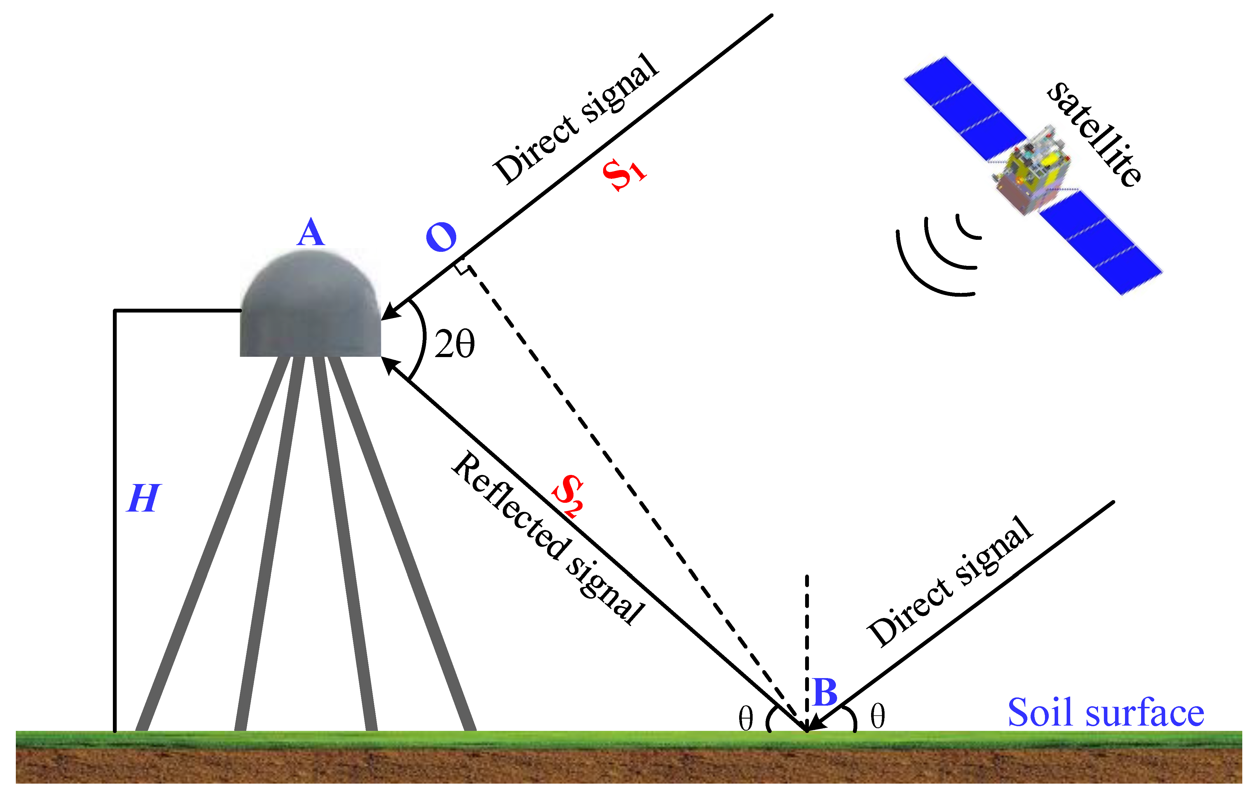
2.1.1. GNSS Multipath Error Principle

In the actual measurement, the signal received by the GNSS receiver antenna is not only the signal directly from the satellite but also the signal reflected by the surface. The direct and the reflected signals entering the receiver antenna interfere with each other, which causes the observation value to deviate from the actual value and produce the multipath error. According to the roughness of the reflective surface of the ground, the two main types of reflection are diffuse reflection and specular reflection [22,24]. For convenience, we assume that multipath error is only caused by specular reflections. Figure 1 shows that direct signal and reflected signal generate corresponding interference effects at the receiver to form a composite interference signal.
The elevation of the GPS satellite ( θ ) determines the path delay Δ S , which is the extra distance travelled by the reflected signal compared to that of the direct signal.
Δ S = 2 H sin θ ,
By substituting carrier wavelength λ into Equation (1), the phase delay δ φ ( t ) corresponding to the path delay can be expressed as:
δ φ ( t ) = 2 π Δ S λ = 4 π H λ sin θ ( t ) ,
where λ is the carrier wavelength; t is the observation epoch. The phase delay is related to the antenna height, carrier wavelength and satellite elevation angle; that is, for a given antenna height and carrier signal, the phase delay is a function of the elevation angle. Equations (1) and (2) only consider the geometric delay and ignore the phase contribution of the Fresnel reflection and antenna radiation.
The amplitude A C and phase difference β ( t ) of the reflected signal compared to the direct signal can be expressed as:
{ A C = A d 2 + A m 2 + 2 A d A m cos δ φ ( t ) β ( t ) = tan 1 [ κ sin δ φ ( t ) 1 + κ cos δ φ ( t ) ] ,
where A m = κ A d , κ is the amplitude attenuation factor (AAF); S C is the composite signal; A C is the amplitude of S C . The factor β ( t ) is the composite excess phase with respect to the direct phase, which can be approximately expressed as [21]:
β ( t ) = ( A m A d ) sin δ φ ( t ) = κ sin δ φ ( t ) ,
When only specular reflection is considered, the composite signal formed by the superposition of the direct signal and the reflected signal S C can be expressed as [21]:
S C = S L + S M = A d cos ( ω 0 t ) + A m cos [ ω 0 t + δ φ ( t ) ] = A C cos [ ω 0 t + β t ] ,
where S L and S M are the direct and reflected signals, respectively; A d and A m are the amplitudes of the direct and reflected signals, reflectively; ω 0 is the angular frequency of the signal.

2.1.2. Calculation of Multipath Error of Linear Combination of Observations

If only the influence of atmospheric delay error is considered, the GNSS code measurement pseudorange and carrier phase observation equation can be approximately described as [25]:
P i = ρ + c ( δ t R δ t S ) + T + I i + E + M P i + ε p i ,
λ i φ i = ρ + c ( δ t R δ t S ) + T I i + E + M φ i + ε φ i λ i N i ,
where i is the carrier number; φ is the carrier phase observation value; ρ is the geometric distance between the receiver and the satellite; c is the propagation velocity of electromagnetic waves in a vacuum; δ t R and δ t S are the clock difference between the receivers and satellite clock, respectively; N is the ambiguity of the whole week; λ is the carrier wavelength; M P and M φ are the pseudorange and carrier multipath error, respectively; T and I are the tropospheric and ionospheric delay errors, respectively; ε represents other unmodeled errors.

2.1.3. Error Calculation of Dual-Frequency Pseudorange Multipath

As shown in Equations (6) and (7), when i is 1 and 2, Equations (6) and (7) can be differentiated, respectively. Considering | M P i | | M φ i | , | ε p i | | ε φ i | is as shown in Equations (8) and (9).
P 1 λ 1 φ 1 = 2 I 1 + M P 1 + ε φ 1 + λ 1 N 1 ,
P 2 λ 2 φ 2 = 2 I 2 + M P 2 + ε φ 2 + λ 2 N 2 ,
The relationship between carrier frequency f and ionospheric delay I is:
I 2 = f 1 2 f 2 2 I 1 ,
By subtracting the L1 and L2 carrier phase observation equations and taking into account Equation (10), we obtain:
λ 1 φ 1 λ 2 φ 2 = I 2 I 1 + λ 1 N 1 λ 2 N 2 = ( f 1 2 f 2 2 1 ) I 1 + λ 2 N 2 λ 1 N 1 ,
Therefore, as shown in Equation (12):
I 1 = ( λ 1 φ 1 λ 2 φ 2 + λ 1 N 1 λ 2 N 2 ) × f 2 2 f 1 2 f 2 2 ,
Therefore, the pseudorange multipath error equation at L1 band is:
M P 1 = P 1 λ 1 φ 1 2 I 1 ε P 1 λ 1 N 1                                       = P 1 f 1 2 + f 2 2 f 1 2 f 2 2 λ 1 φ 1 + 2 f 2 2 f 1 2 f 2 2 λ 2 φ 2 + K ( N 1 , N 2 , ε P 1 ) ,
Similarly, the pseudorange multipath error equation in L2 band is:
M P 2 = P 2 2 f 1 2 f 1 2 f 2 2 λ 1 φ 1 + f 1 2 + f 2 2 f 1 2 f 2 2 λ 2 φ 2 + K ( N 1 , N 2 , ε P 2 ) ,
where M P 1 and M P 2 are the multipath errors of the L1 and L2 carriers, respectively; P 1 and P 2 are the pseudorange observations of the L1 and L2 carriers, respectively; f 1 and f 2 are the frequencies of the L1 and L2 carriers, respectively; λ 1 and λ 2 are the L1 and L2 carrier wavelengths, respectively; φ 1 and φ 2 are the observed values of L1 and L2 carrier phases, respectively; N 1 and N 2 are the ambiguities of L1 and L2 carriers, respectively; ε P 1 and ε P 2 are other unmodeled errors.
In Equations (13) and (14), K ( N 1 , N 2 ) is the integer ambiguity combination, which is usually a constant and does not affect the overall trend in the pseudorange multipath error. If no cycle slip occurs, it can be omitted. Therefore, the main factors affecting the quality of pseudorange multipath error are the noise in pseudorange observations and the accuracy of carrier phase observations and code pseudorange observations. If cycle slip occurs in carrier phase observations, it affects the value of pseudorange multipath error. Therefore, for the pseudo-range multipath error in each period, cycle slip detection and repair are required. We selected the multipath error M P 2 of the L2 carrier as the research object.
The dual-frequency pseudorange multipath can be calculated by the linear combination of the pseudorange observations and the carrier phase observations, which can be expressed as [26]:
M P 1 = P 1 f 1 2 + f 2 2 f 1 2 f 2 2 λ 1 φ 1 + 2 f 2 2 f 1 2 f 2 2 λ 2 φ 2 ,
M P 2 = P 2 2 f 1 2 f 1 2 f 2 2 λ 1 φ 1 + f 1 2 + f 2 2 f 1 2 f 2 2 λ 2 φ 2 ,

2.1.4. Multipath Error Calculation of Dual-Frequency Carrier Phase Linear Combination

For carrier phase observables, isolating the multipath from several other effects, such as the satellite antenna pseudorange and ionospheric and tropospheric delay, is difficult. However, when considering the multipath, the carrier phase contains two quantities: the phase of the direct signal and the composite excess phase with respect to the direct phase. Thus, the GNSS phase observation for carriers L1 and L2 can be expressed as [27]:
{ L 1 = λ 1 ψ 1 + λ 1 β 1 ( t ) L 2 = λ 2 ψ 2 + λ 2 β 2 ( t )
where ψ 1 and ψ 2 represent the phase of the direct signal; β 1 ( t ) and β 2 ( t ) are the composite excess phase with respect to the direct phase.
In GNSS positioning, the carrier phase of the direct signal can be expressed as:
λ i ψ i = ρ + I i + T + Δ ,
where i = 1 or 2, which is the two signals with different frequencies. The geometric distance between the GNSS satellite and antenna is represented by ρ , I i represents ionospheric delays, T represents tropospheric delays, and Δ accounts for all other carrier-independent effects. To isolate the multipath, the dual-frequency carrier-phase combination L4 is the L 1 L 2 combination of carrier phase measurement, and its mathematical expression is [9,27]:
L 4 = L 1 L 2 = I 1 I 2 + λ 1 β 1 ( t ) λ 2 β 2 ( t ) ,
Equation (19) eliminates the satellite clock error, receiver clock error, and tropospheric delay, as well as the geometric distance between the satellite and the receiver. That is the observed value of L4 is affected by both ionospheric delay and phase error. Therefore, when analyzing the multipath error, a suitable method must be adopted to weaken the influence of the ionospheric delay on the multipath error. The high-order polynomial is used to fit the L4 multipath error, and the dual-frequency linear combination multipath error that is not affected by ionospheric delay is obtained, which is the L4-free (L4_IF) observation value.

2.2. Establishment of Model Error Equation

According to Equations (1) and (2), the phase delay and path delay are functions of the elevation angle and reflector height. The reflector height changes with the SMC, which contributes to the change in the phase delay and path delay [12]. demonstrated that the agreement between H and the SMC was not as strong as that between δ φ ( t ) and the SMC. Therefore, the phase delay can be used to characterize the change in the SMC. To accomplish this, Equation (5) must be linearized first. Thus, the error equations can be expressed as:
β ( t ) + V β ( t ) = κ 0 sin δ φ 0 + sin δ φ 0 V κ + κ 0 cos δ φ 0 V δ φ ,
where β ( t ) can be easily calculated through Equations (16), (17) and (19). V β ( t ) is the residuals corresponding to the DFP multipath error and L4_IF multipath error. κ 0 denotes the initial value of the AAF. The initial value of the phase delay, i.e., δ φ 0 , can be calculated by incorporating the wavelength ( λ ), antenna height ( H ), and elevation angle ( θ ) into Equations (1) and (2), respectively. V κ and V δ φ are two unknown correction parameters corresponding to κ 0 and δ φ 0 that need to be solved. To ensure the reliability of the solution and to avoid the influence of the excessive difference in multipath errors on the correction parameter solving, we assumed that the SMC remained the same in the short term (e.g., within 5 min) and employed a total of 11 multipath errors to solve the correction parameters through unweighted least squares adjustment. It is worth mentioning that the number of multipath errors is not limited to 11, but should be greater than or equal to the number of the correction parameters to be solved.

2.3. Solving the Phase Delay

The least-squares adjustment method is used to solve the delay phase. The L4_IF method is taken as an example to illustrate the solving process of the phase delay. For the 11 multipath errors of one observation session for a single GPS satellite, 11 error equations, such as Equation (20), can be obtained. Then, these error equations can be expressed by the following matrix:
V β ( t ) 11 × 1 = A 11 × 2 X 2 × 1 l 11 × 1 ,
where
V β ( t ) 11 × 1 = [ V β 1   V β 2   V β 3     V β 11 ] T ,
X 2 × 1 = [ V k   V δ φ ] T ,
A 11 × 2 = [ sin δ φ 0           sin δ φ 0         sin δ φ 0         sin δ φ 0 κ 0 cos δ φ 0       κ 0 cos δ φ 0       κ 0 cos δ φ 0       κ 0 cos δ φ 0 ] T ,
l 11 × 1 = [ β 1 κ 0 sin δ φ 0   β 2 κ 0 sin δ φ 0   β 3 κ 0 sin δ φ 0     β 11 κ 0 sin δ φ 0   ] T ,
where β ( t ) represents the L4_IF multipath error, V β ( t ) is the residual for β ( t ) . The subscripts 1, 2, 3, …, 11 denote the serial number of the selected 11 multipath errors. Thus, based on unweighted least-squares adjustment ( V T V = min). X can be obtained by the following formula.
X = [ V κ V δ φ ] = ( A T A ) 1 × ( A T l ) = N 1 2 × 2   W 2 × 1 ,
where N = A T A ; W = A T l . Because its rank equals one, N is rank deficient, which leads to a non-unique solution of X . Therefore, to obtain a unique solution, pseudo-inverse adjustment was adopted.
X = [ V κ V δ φ ] = N 2 × 2   W 2 × 1 ,
where N 1 and N is the Kelley inverse and the pseudo-inverse of N , respectively. Thus, the adjusted phase delay and AAF can be obtained:
[ κ ^ δ φ ^ ] = [ κ 0 + V κ δ φ 0 + V δ φ ] ,
The diurnal phase delay representing the trend of the soil moisture change, namely the mean of the adjusted phase delay of twelve observation sessions, can be obtained by the following formula:
δ φ ¯ i = δ φ ^ i , 1 + δ φ ^ i , 2 + δ φ ^ i , 3 + + δ φ ^ i , 12 12 ,
where the subscript i equals 1, 2, 3, …, 78, and represents the i th day; the numbers 1, 2, 3, …, 12 represent the serial number of observation sessions on a single day.

2.4. Data Sources

The experimental data are from the USA. Plate Boundary Observatory (PBO). We selected the GPS observation data of the P041 station (Figure 2) and the SMC data collected by the P041 and MFLE stations (https://cires1.colorado.edu/portal/) (accessed on 10 September 2021). The days of the year (DOYs) of selected observation data are between 45 and 131 of 2014 (Note: 57, 67–69, 71, 82, 94, 104, 105 days of soil moisture data are missing and have been eliminated).
The PBO SMC consisted of the site averaged SMC on a daily timescale, and the median SMC value of all satellite tracks for each day was used [22]. (https://data.unavco.org/archive/gnss/products/) (accessed on 15 September 2021). Located in Colorado, USA, and positioned at an altitude of 1728.8 m, the P041 station (39.9495°N, 105.1943°W). The MFLE station is about 210 m away from the P041 station, its altitude is 1727.3 m, and its position is longitude and latitude (39.9476°N, 105.1944°W). The soil moisture data of the MFLE station is used to further verify this method’s reliability. In view of this, this paper takes P041 station as the research station, MFLE station as the verification station, and MFLE station is very close to P041 station, as shown in Figure 2. The surrounding environment of P041 and MFLE stations are shown in Figure 3 (https://www.unavco.org) (accessed on 25 September 2021). The GNSS receiver and related parameters of the P041 station are shown in Table 1.
The P041 and MFLE stations can be seen in Figure 3a,b, respectively. They are located in a flat and open area, and the surrounding vegetation is scarce, and the land cover consists of exposed soils and short grasses. This paper selects the experimental data for the late winter and early spring. Therefore, the surface reflection signal is less affected by vegetation attenuation.
Figure 4 shows the observed SMC and precipitation data series corresponding to the time (DOYs: 45-131,2014) of selecting GNSS observation data from P041 and MFLE stations, which are presented in a line graph and a histogram, respectively. As demonstrated in Figure 4, six significant indigenous precipitation events occurred during the experiment, with a maximum precipitation of 24.8 mm, mainly during DOYs 63–66, 92–93, 102–103, 109–110, 127–128 and 130–131. Continuous precipitation led to a significant nonlinear increase in the SMC. As precipitation decreased or stopped, there was a decrease in the SMC. Evidently, precipitation was the primary factor that caused sudden changes in the SMC. The precipitation at the P041 and MFLE stations during the experimental period was appropriate and suitable for SMC retrieval.

3. Experiment and Results

3.1. Experimental Technical Scheme

Figure 5 shows the flow chart of the SMC retrieval technique used in this study. The technical route we followed can be divided into three parts: (1) We first pre-processed the GNSS-IR data: the carrier phase, pseudorange observation data, azimuth, elevation angle, and epoch extraction. We extracted other data parameters from the observation (OBS) file and navigation (NAV) file collected by GNSS receivers. (2) We determined the initial values of phase delay and amplitude attenuation factor, then constructed the dual-frequency carrier phase linear combination multipath error model and dual-frequency pseudorange multipath error model, and then calculated the multipath errors of the two models separately. We fit the ionospheric linear combination (L4), namely the simple difference between L1 and L2 ( L 4 = L 1 L 2 ), with a high order to obtain L4_IF. We used a 10-degree polynomial fitting. (3) By constructing the error equation, we solved the delay phase. Then, we performed the delayed phase combination representing the variation trend in SMC and the retrieval SMC analysis. (4) Taking the multipath error of the five epochs before and after as the observation value, we calculated the dual-frequency pseudorange multipath error and the dual-frequency carrier-phase combination error and determined the initial phase and the amplitude attenuation factor (AAF). According to Equation (5), we established the model error equation. We used the Lomb–Scargle periodogram (LSP) and least-squares adjustment method to solve the delay phase. In solving the delay phase, the Pearson correlation coefficient (R) between the phase delay and SMC was used to characterize the changing trend between the delay phase and soil moisture.

3.2. SMC Retrieval

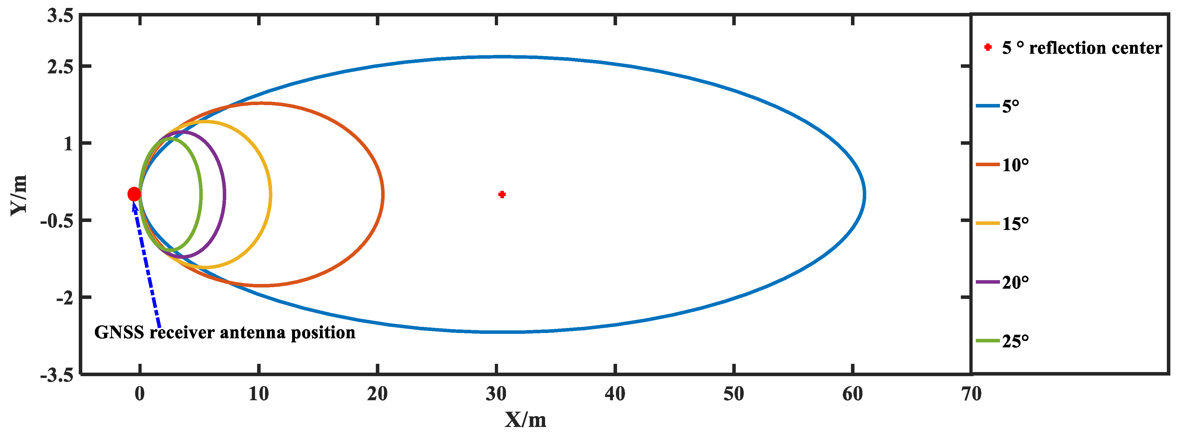
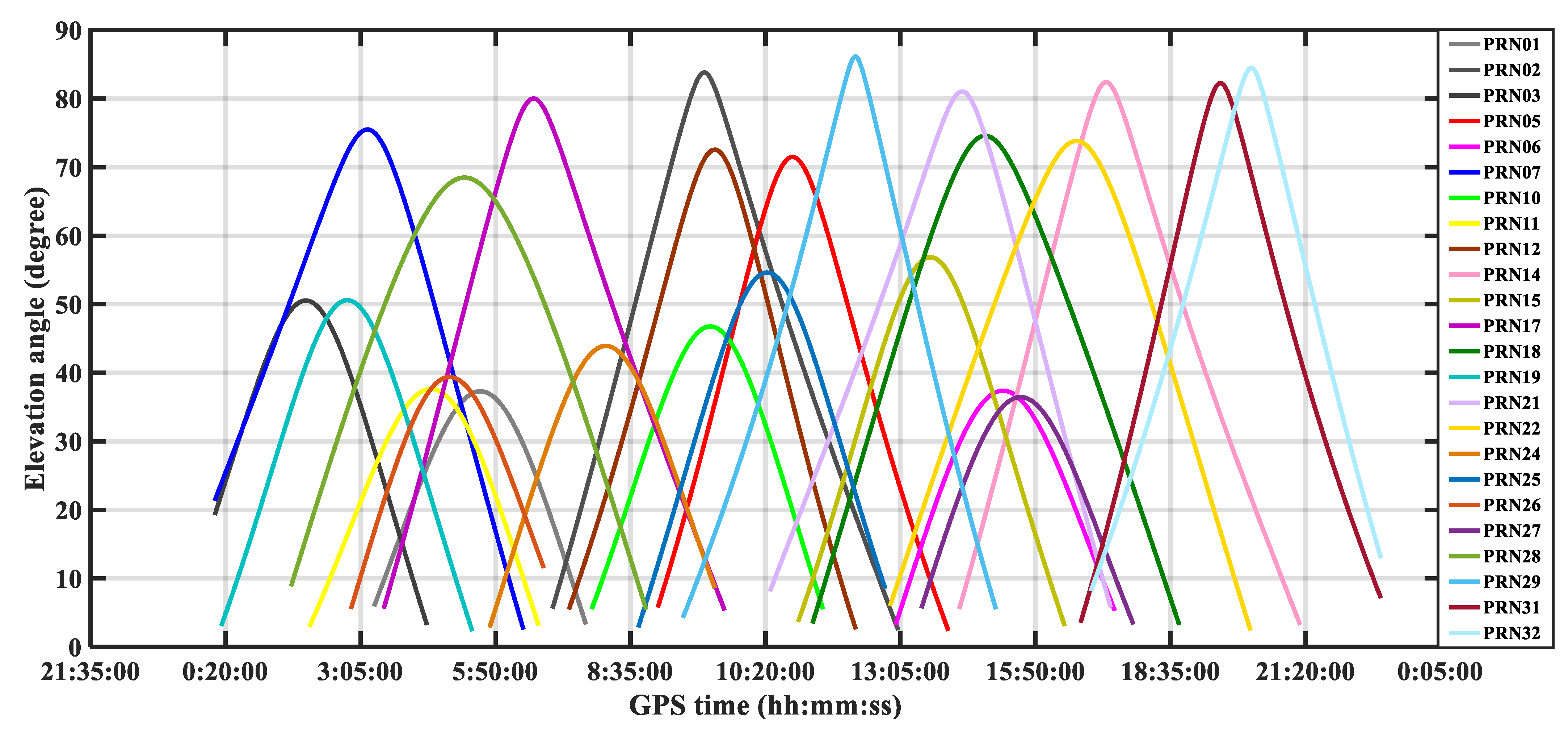
3.2.1. Choice of Elevation Angle

Given the lack of measured soil moisture data, we selected the soil moisture value from the P041 station estimated with the new GPS L2C carrier SNR as the reference value. The soil moisture value of the PBO site is based on a value per day and is the median value estimated by all satellites [22]. As soil moisture changes more during the day than that at night and more GPS satellites are visible during the day than at night, to simplify the calculation, generally, only four and eight observation periods are selected at night and day, respectively. As such, we used twelve observation periods every day. To ensure the solution’s reliability and avoid excessive differences in multipath errors from affecting the parameter solution, we assumed that the soil moisture remained constant for a short time (e.g., within 5 min). We used the multipath error of the element used as the observation value for 11 multipath errors in total.
To provide a more intuitive view of the number of GPS satellites visible during the day compared to at night, Figure 6 shows the change in elevation of almost all GPS satellites at site P041 on 19 February 2014 (DOY: 2014–050). Figure 6 shows that more GPS satellites are visible during the day than at night, and the duration of a single GPS satellite being visible during l day is generally about 2.5–8 h, and the period at a low satellite elevation angle (<30°) is shorter, being maintained at about 0.5–2 h.
Figure 7 shows the linear combination of GPS satellite G22 (DOY: 2014-050) observations at the test site. The multipath error varied with the elevation angle of the satellite. The black curve represents the change trend in MP2 multipath error and L4_IF multipath error over time, and the red parabola represents the change trend in satellite elevation angle with time. Figure 8 shows that the satellite elevation angle occurs between 13:30 and 21:30. The time gradually increases to the maximum value and then slowly decreases until the satellite disappears. The changes in the MP2 multipath error and L4_IF multipath error are closely related to the satellite elevation angle. When the satellite elevation angle is low, the MP2 value oscillation amplitude can reach several meters, and the L4_IF value oscillation amplitude is relatively large. When it is high, the oscillation amplitudes of the MP2 value and L4_IF value decrease accordingly. For increased accuracy, we selected the data at the lower elevation angle as the experimental data, as shown in Figure 8.
Figure 8 shows the multipath error of the linear combination observations of the GPS satellite G22 (DOY: 2014-050) at a satellite elevation of 5–25° for the test site GPS satellite. Figure 8 shows that as the satellite elevation angle increased, the multipath error showed a downward trend, which indirectly indicated that the carrier pseudorange and carrier phase observations of low-elevation satellites are more susceptible to the influence of multipath errors; it provides a theoretical basis for the selection of GNSS-IR satellite altitude angle. The satellite elevation angles in this experiment were all limited to 5–25°.

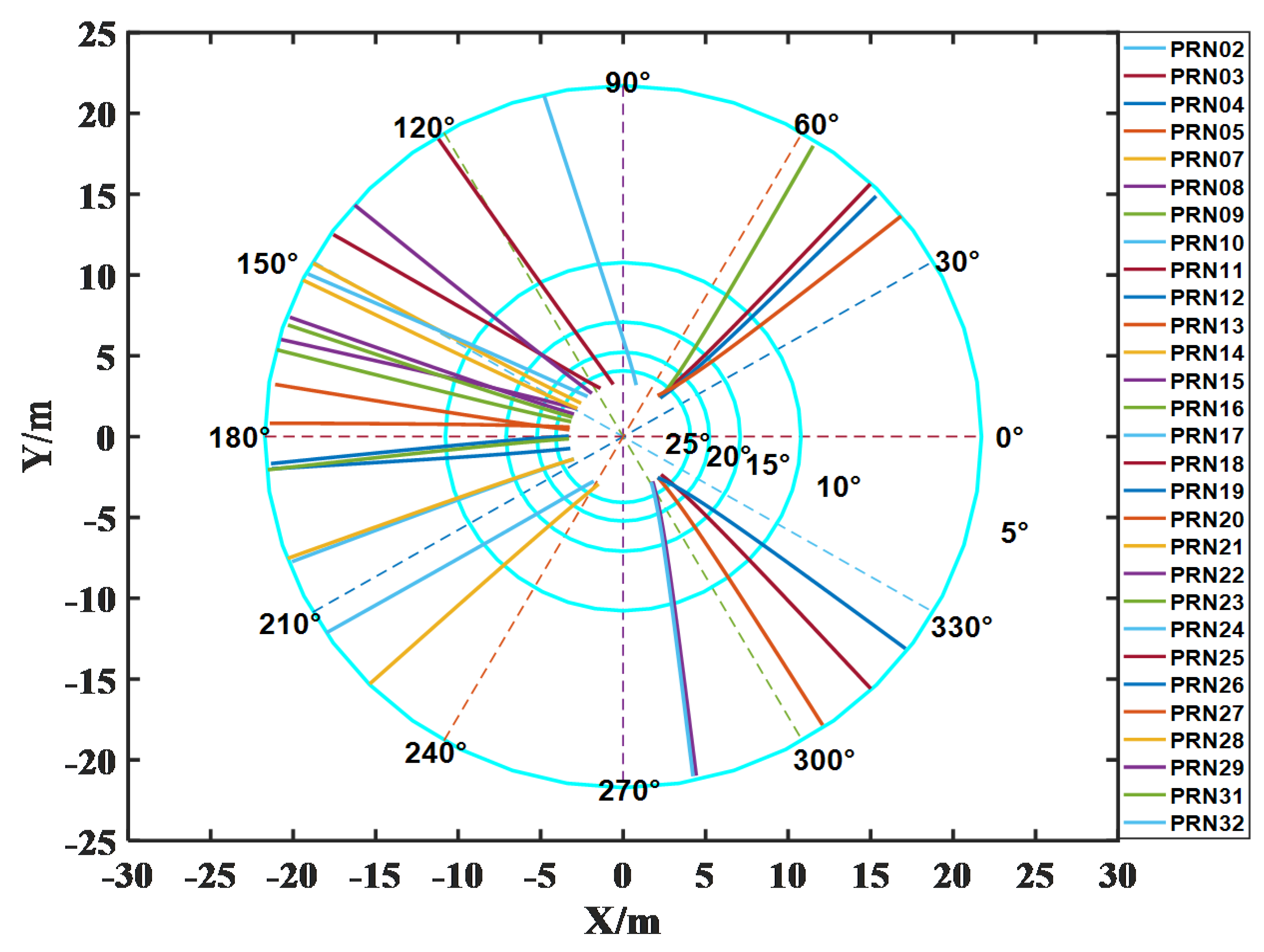
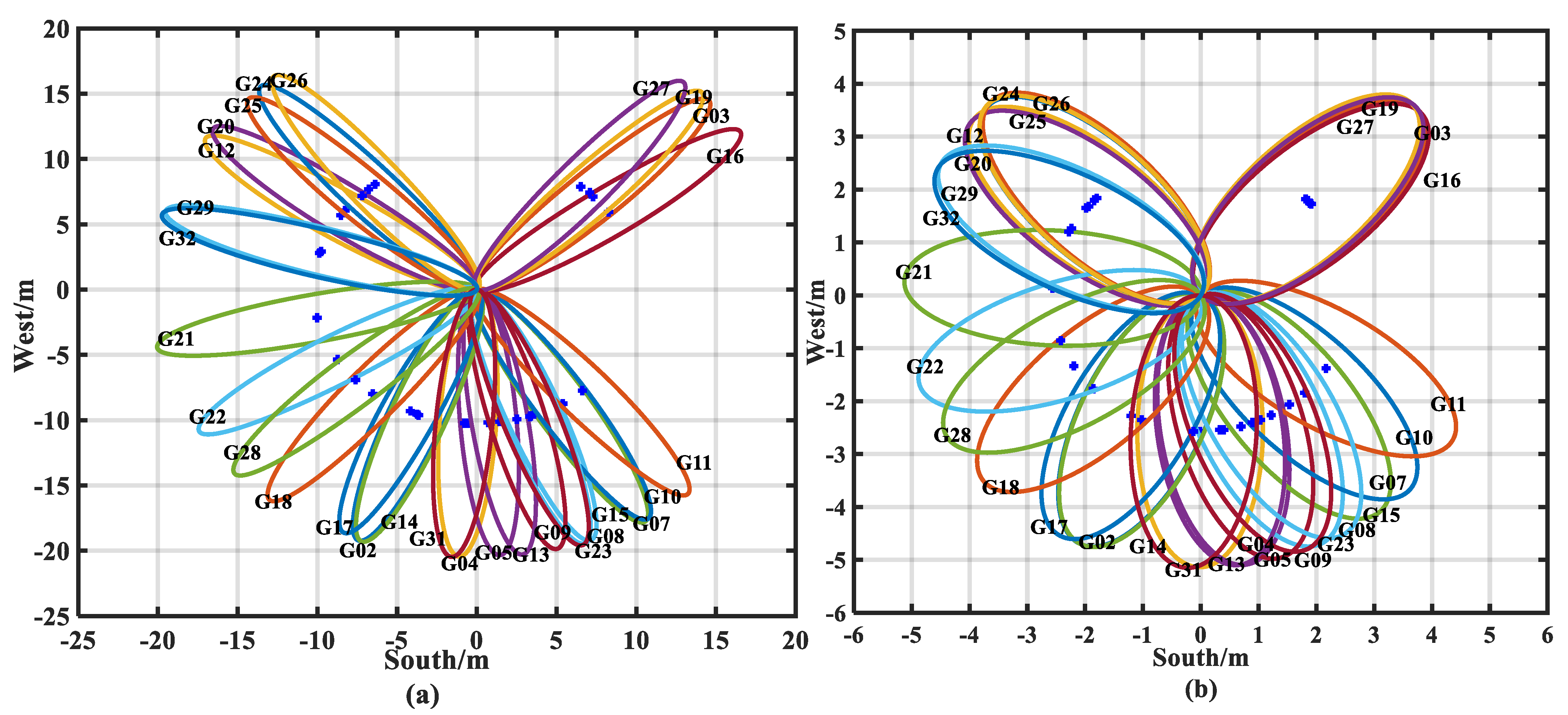
3.2.2. Choice of Azimuth

Satellite signal reflection point trajectory is a function of satellite elevation, azimuth, and antenna height. The reflection point trajectory reflects the position of the satellite relative to the receiver at a certain moment, from which the spatial information of the reflected soil can be obtained. Therefore, the advantages of the satellite reflection point trajectory map can be used, and the satellite azimuth angle can be considered to ensure as much consistency of the multiperiod multipath environment as possible. We selected the area with more visible satellites as the azimuth angle range at the experimental site.
Given the spatial differences in soil moisture and surface environment in the study area, the soil moisture at different locations was not entirely consistent, which led to the difference between the retrieval results based on the observation values at different reflection locations. In addition, not all DFP observations and L4_IF observations of the satellite elevation state contain the physical information of the surface reflector. Therefore, we needed to select observation values based on the study area environment, satellite elevation angle, and satellite azimuth angle to improve the accuracy of GNSS-IR soil moisture retrieval. As shown in Figure 9, as the reflection area of the soil was roughly the same, and on the premise of ensuring the number of satellites in each period, we selected an azimuth angle range of 30–330°. The satellites all had continuous observation values when their elevation angle was 5–25°, providing relatively sufficient observation data.

3.2.3. Selection of Effective Satellites

The Fresnel reflection region of a GNSS signal is a set of ellipses related to the elevation, azimuth, and antenna height of a satellite. The first Fresnel reflection region contributes the most to the reflected signal, and the reflection medium change in the reflection zone strongly affects the relevant physical characteristics of the reflected signal.
The semimajor and semiminor axes of the ellipse of the first Fresnel reflection region of the ground-based GNSS-R can be determined by [28]:
S x = h cot θ ,
S y = 0 ,
a = λ h sin   θ sin 2 θ ,
b = λ h sin θ sin θ ,
where S x is the projection position of the reflection point on the ground connecting the satellite and the receiver; S y is the position of the receiver projection point; a and b are semimajor and semiminor axes of the first Fresnel reflection region; h is the distance from the antenna phase center to the reflection surface; λ is the carrier wavelength; θ is the elevation angle of the GNSS satellite.
Figure 10 shows the first Fresnel reflection region ellipse group of the GPS L2 carrier when the satellite azimuth was 0°, the satellite elevation was 5–25°, and the receiver antenna height was 1.9 m. The horizontal axis represents the distance from the receiver antenna to the direction of the satellite, and the vertical axis represents the distance perpendicular to the direction of the receiver antenna and satellite. When the satellite elevation angle increases, the Fresnel reflection region shrinks, and the reflection center is closer to the GNSS receiver. The area of the ellipse can be obtained from the semimajor and semiminor axes of the ellipse, that is, the area of the first Fresnel reflection region. Using the first Fresnel reflection region can avoid the influence of other multipath sources, such as tall buildings, vegetation, and water; maximize the unity of the reflection medium in the reflection zone; and be used for the design of the experimental plan. Therefore, the Fresnel reflection region provides a certain basis for determining the location of soil moisture sample collection points and selecting effective satellites. The change in the reflection medium in the Fresnel reflection region considerably affects the signal received by the receiver.
Figure 11 shows the first Fresnel reflection region map of station P041 (DOY: 2014-065). When the satellite elevation angle was 10°, the reflection point was up to 21 m away from the receiver. If slopes or other interference sources are near the measurement area, the first Fresnel reflection region should be introduced to reduce the excessive soil moisture retrieval error caused by different soil reflection media. The lower the satellite elevation angle, the larger the region of the first Fresnel reflection. When the elevation angle range is limited, the azimuth angle of each GPS satellite does not change much. Therefore, the calculation of the first Fresnel reflection region can ensure the unity of the medium in the reflection region, meaning that the homogeneity of the soil can be more accurately assessed and can provide a certain basis for other factors such as experimental planning and satellite selection.
The maximum power spectral density can be used to characterize the quality of a multipath error signal to a certain extent. Spectrum analysis using the Lomb–Scargle method can be used to judge satellite signal quality [22,29]. A satellite track should have a relatively stable singular dominant frequency for the same reflecting surface. In general, the dominant frequency’s power spectral density (PSD) should be at least twice as high as the power of the noise or the second most powerful frequency in the periodogram [22,30].
Figure 12a,b show that the power that meets the dominant frequency should be at least twice the power of the secondary main peak frequency, and that the quality of satellite data is higher. We used the PSD of dual-frequency pseudorange and dual-frequency carrier phase combined multipath error as the main auxiliary tool for satellite selection. Figure 12c,d lack any dominant frequency, which could have introduced substantial errors in the subsequent parameter estimation. Therefore, we also discarded such satellites when selecting satellites.
Based on the above analysis, after limiting the satellite elevation angle to about 5°–25° and after further considering the dual-frequency multipath error for satellite selection, we used twelve time periods every day: eight evenly distributed in the daytime and four and evenly distributed in the nighttime. Although the multipath error duration of a single GPS satellite in a day is generally about 2–8 h, the corresponding duration of the low satellite elevation angle multipath error is shorter, basically maintained at about 1 h. As a result, even fewer GPS satellites are available at low elevations. Therefore, we selected only one GPS satellite for each observation period. Combining satellite elevation angle, satellite reflection trajectory, satellite azimuth, first Fresnel reflection area, station environment, spectrum analysis, etc., Table 2 shows the results of the twelve time periods on 6 March 2014.

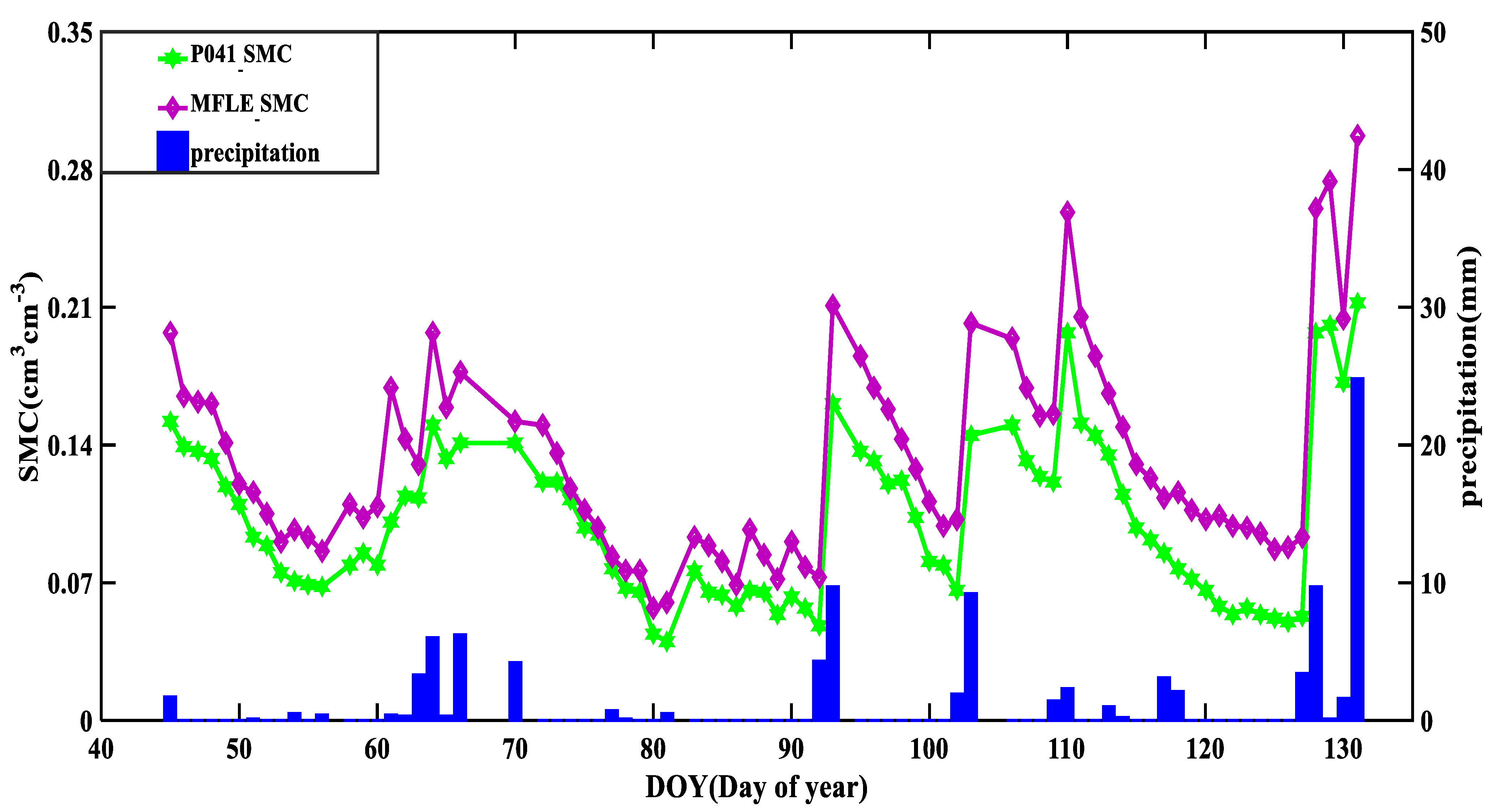
3.3. GNSS-IR SMC Retrieval Results

To obtain the parameters that characterize the change trend in soil moisture, we used the multipath error as the system input, and the amplitude attenuation factor and phase delay were the parameters to be estimated. We ignored the impact of the satellite elevation, soil moisture changes in the short term, and the amplitude attenuation factor and phase. The delay was a constant in the short term, and we obtained the error equation by linearizing Equation (5). The initial value of the phase delay was determined using Equation (2), where the satellite elevation angle is the satellite elevation angle corresponding to the first soil moisture sample collection time, considering that the soil surface reflectivity is between 0.3 and 0.8 [21]. In this study, we focused on the amplitude and phase of multipath error, so the actual value of κ is not required. Taking an κ initial value κ 0 = 0.3 , we ignored the complex effect of antenna gain mode.
Considering the small changes in the sine values of antenna height and satellite height and our focus on the changing trend in the phase delay, we used the same initial phase delay value for all periods of data processing. For the solution of the parameters, we adopted the indirect adjustment method based on least squares, and the data processing followed these principles:
(1)
Cycle slip detection and repair were conducted on the observed carrier phase value;
(2)
We assumed that the amplitude attenuation factor and phase delay did not change in a short time;
(3)
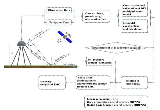
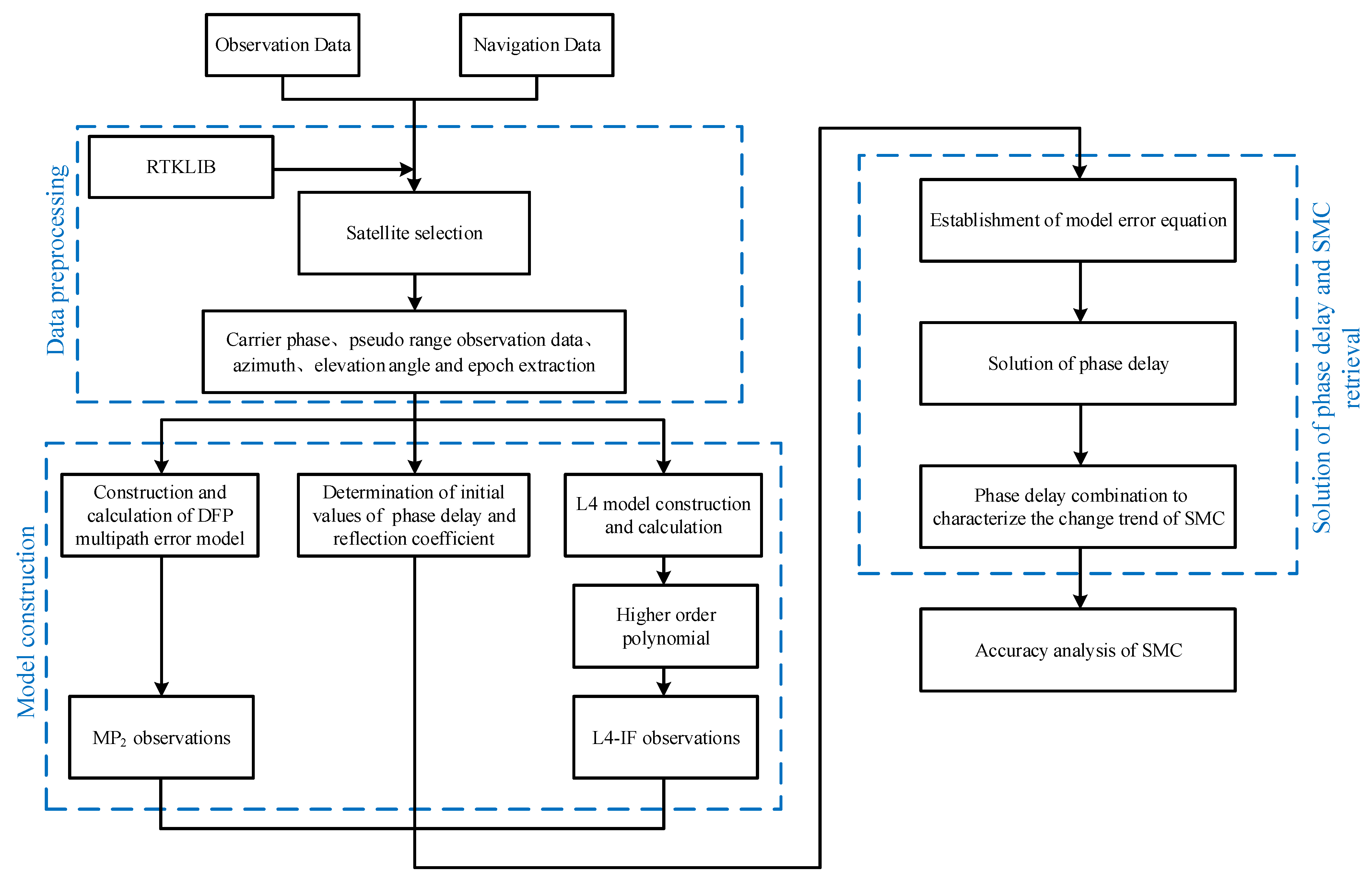
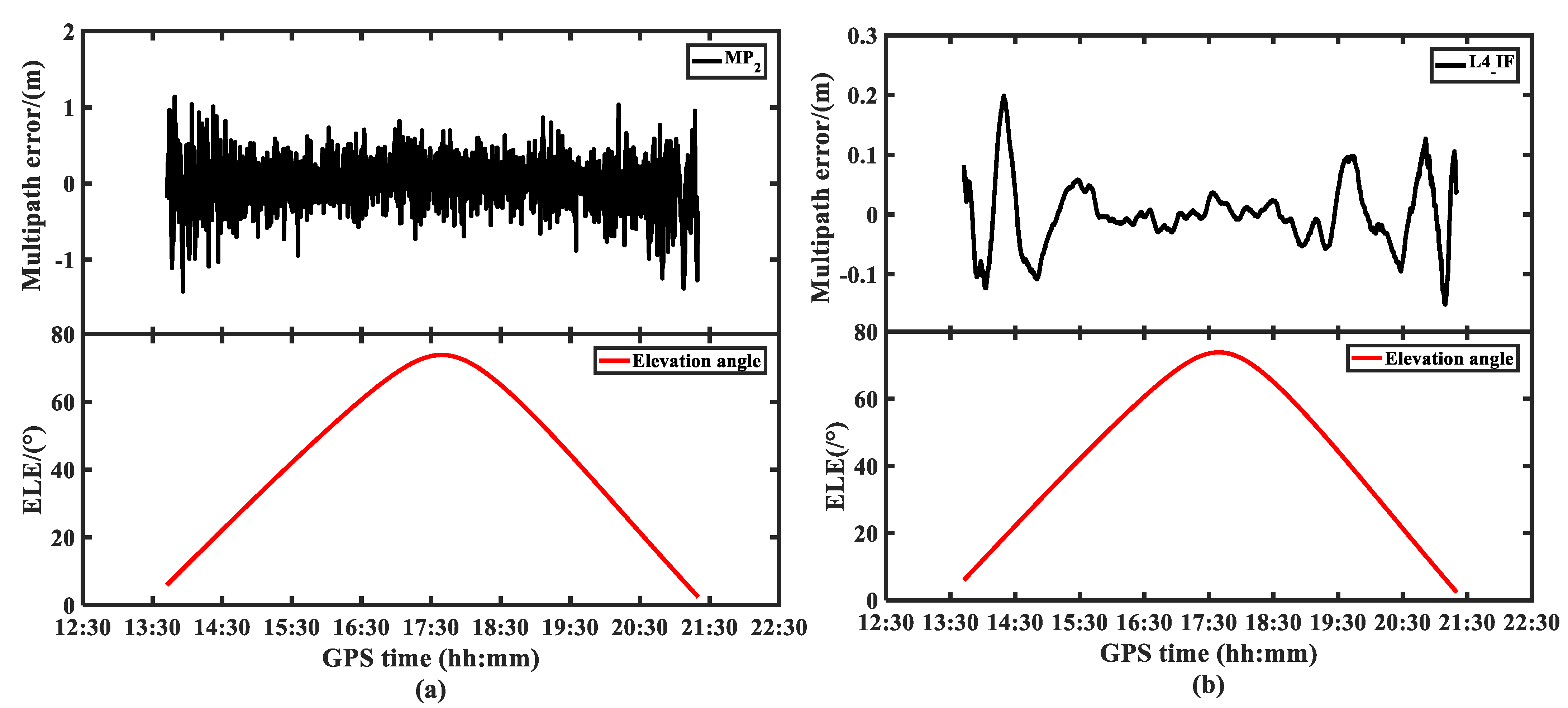
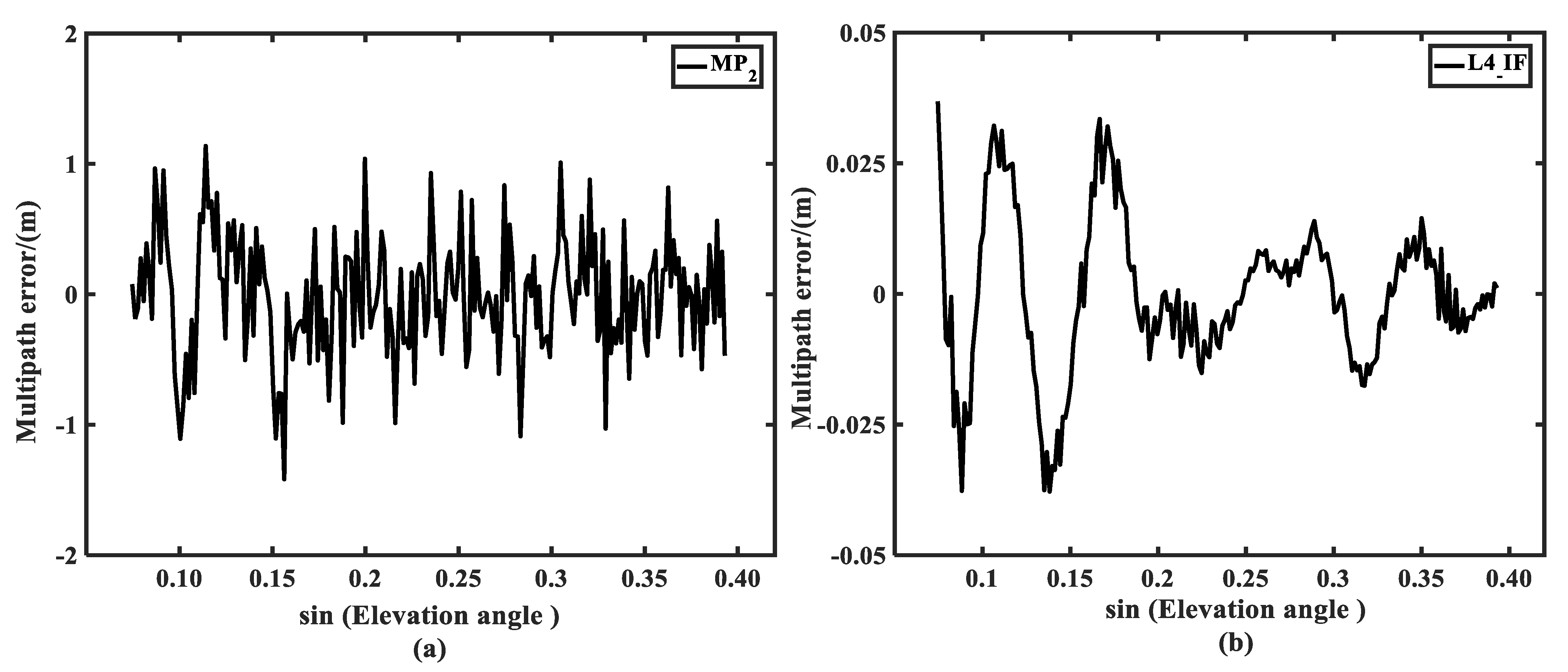
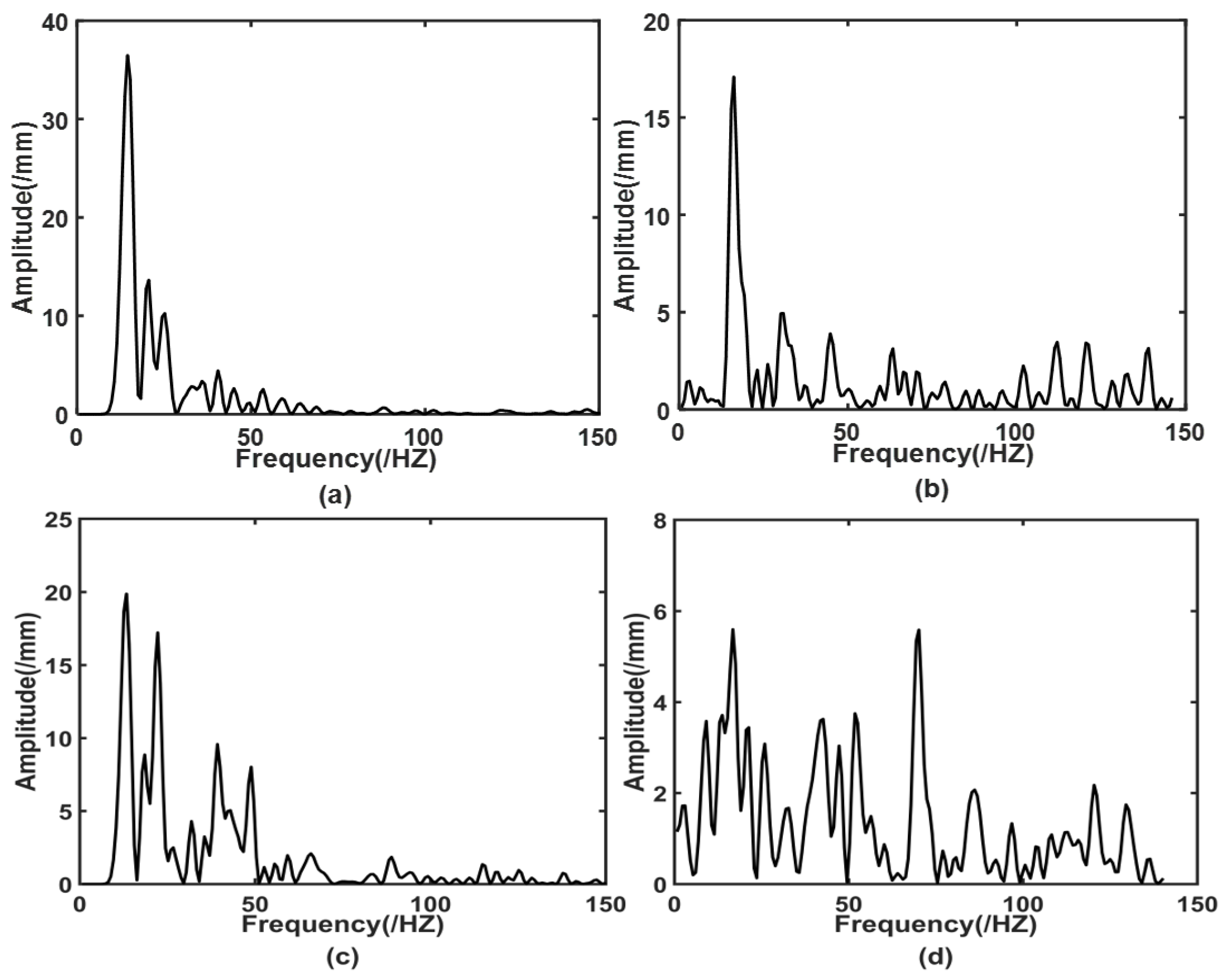
To avoid the large difference between the delay phase and the acquisition time of soil moisture, considering the necessary observation number, taking the acquisition time of soil moisture as a reference, we took the multipath error of five epochs before and after as the observation value. That is, we ignored the change in the delay phase with satellite elevation angle in the short term. We regarded the multipath error selected in each period as the repeated observation of the same parameter. According to Equations (15) and (16), the dual-frequency pseudorange multipath error MP could be calculated; According to Equation (19), the dual-frequency carrier-phase combination multipath error L4 could be calculated. We performed high-order fitting (we used 10-degree polynomial fitting) of L4 to remove the influence of ionospheric delay and obtain L4_IF. According to Equation (2), the initial value of the delay phase and the initial value of AAF ( κ 0 ) are determined. According to Equation (5), we constructed the error equation of the corresponding method, and performed the Lomb–Scargle periodogram (LSP) and least square adjustment method. We solved each period to obtain a delay phase representing the change trend in soil moisture.
Combining the results of daily satellite selection, for the selected single satellite, we calculated the multipath error according to the dual-frequency signal of 11 epochs before and after the corresponding time. Combining the above principles and methods, we obtained the delay phase corresponding to the time of soil moisture acquisition through adjustment. Therefore, one phase delay could be calculated for each observation period, and 12 phase delays could be calculated for 12 observation periods in a day. By averaging the 12 results, we obtained the average phase delay, which is the daily phase delay. On a daily time scale, the L4_IF method and the DFP method were calculated separately to obtain the corresponding daily phase delay, and Time trends of soil moisture and delayed phase at P041 and MFLE stations were plotted (Figure 13a,b and Figure 14a,b).
To further test the L4_IF method and the DFP method, 50 d of the P041 and MFLE SMC, respectively, and the estimated phase delay were employed to build an empirical model, and the other 28 d of data were used to verify the model. The modelling method employed was unary linear. In the relationship between soil moisture and phase delay, in this study, we used the phase delay as the independent variable (x) and the soil moisture as the dependent variable (y) to perform univariate linear regression modeling. We obtained the scatter plot and regression shown in Figure 15.
To better reflect the soil moisture retrieval performance of the two methods of P041 and MFLE stations, we performed precision statistical analysis on each method separately, and the statistical results are shown in Table 3.
Soil moisture is often affected by vegetation cover, soil temperature, air humidity and other factors. In addition, due to the difference between the actual reflection conditions of GNSS satellite signals and the hypothetical ideal reflection conditions, the relationship between multi-path induced phase delay and soil moisture becomes complicated, which makes the ordinary linear model not necessarily able to describe the trend of soil moisture. Compared with other analytical models, the neural network model is less sensitive to the influence of soil flatness, surface vegetation and soil surface roughness. Therefore, in order to improve the inversion accuracy of GNSS-IR soil moisture, BPNN and RBFNN were used to construct soil moisture prediction models, and the prediction results were compared with those of ULR model, and the accuracy of each model was evaluated.
The phase delay and measured soil moisture of P041 and MFLE stations calculated based on L4_IF method and DFP method were used as data sources, and the training set and test set were divided according to the ratio of 7:3. That is, 50 d data were used as training set data, and 28 d data were used as test set data. BPNN and RBFNN are used to model. Figure 16 and Figure 17 show the comparison between the predicted values of the three models of the two methods corresponding to the P041 station and the MFLE station and the measured values of soil moisture.
In order to better reflect the prediction results of three prediction models for soil moisture and the comparison results between different models, the accuracy of L4_IF and DFP methods corresponding to the three models of P041 and MFLE stations were statistically analyzed. The statistical results are shown in Table 4.

4. Discussion

From the above experimental results can be drawn, Figure 13a,b and Figure 14a,b show multiple apparent peaks in the phase delay and soil moisture, and the overall change trend has a strong consistency. For the P041 station, the correlation coefficients between the soil moisture and phase delay calculated based on the L4_IF multipath error and the DFP multipath error are 0.97 and 0.91, respectively. For the MFLE station, the correlation coefficients between the soil moisture and phase delay calculated based on the L4_IF multipath error and the DFP multipath error are 0.93 and 0.86, respectively, which are statistically significant. Figure 15a–d shows that the soil moisture values obtained using the L4_IF and DFP methods both fluctuate around the linear regression equation built by each, and the deviation is slight. The L4_IF and DFP methods have a statistical significance level of 0.01 and 0.05, respectively, regarding soil moisture retrieval. The probability values of the two methods are close to zero ( P 0 ), indicating that the correlation between the estimated phase delay and soil moisture at the P041 and MFLE stations is significant. Figure 16 and Figure 17 show that the fitting degree between the predicted and measured values of the BPNN model and RBFNN model is better than that of the ULR model, and the error is smaller.
Table 3 shows that the standard deviation and absolute average error of the L4_IF and DFP methods are the same, but the root mean square error of the L4_IF method is smaller than that of the DFP method. Therefore, the L4_IF method is generally more accurate than the DFP method. The observation precision of the carrier phase is much higher than that of the pseudorange. To better compare the L4_IF and DFP methods, we used the error propagation law to compare the error level of L4_IF and DFP. Assuming that the observation error of the dual-frequency carrier phase has the same standard deviation of 1 mm ( σ 0 = σ 1 = σ 2 = 1 mm ), the standard deviation of the GPS C/A code measurement pseudorange observation value is 2.93 m. Therefore, the error standard deviation of the L4_IF method is σ L 4 = 2 σ 0 = 1.41   m m, and that of the DFP method is σ M P 2 = 2.93   m   σ L 4 < σ M P 2 , also means that the quality of the multipath error of the L4_IF method is higher than that of the DFP method, so the L4_IF method obtained a higher correlation coefficient and root mean square error.
Table 4 shows that for the L4_IF and DFP methods of P041 and MFLE stations, the prediction results of the BPNN model are better than the RBFNN model and ULR model, and the RBFNN model is slightly better than the ULR model. The reasons may be as follows. Firstly, soil moisture is affected by vegetation cover, soil temperature, air humidity and other factors, and multipath reflection is not an imaginary mirror reflection, which makes it difficult to characterize other nonlinear characteristics between delay phase and soil moisture by using simple linear or exponential models. Secondly, the BPNN algorithm can correct the dielectric constant difference caused by weakening soil roughness, and has a certain inhibitory effect on surface fluctuation, soil roughness and vegetation.

5. Conclusions

Based on the analysis of the multipath error generation mechanism and the calculation model of GNSS measurement, we constructed a soil moisture retrieval method based on multisatellite dual-frequency combined multipath error. We proposed a method of estimating soil moisture using two combined dual-frequency signals. We used the L4_IF and DFP methods, which are independent of geometric distance, to estimate soil moisture. We verified the proposed method using the archived data set and SMC data of the P041 and MFLE stations. We drew the following conclusions through experimental analysis:
(1)
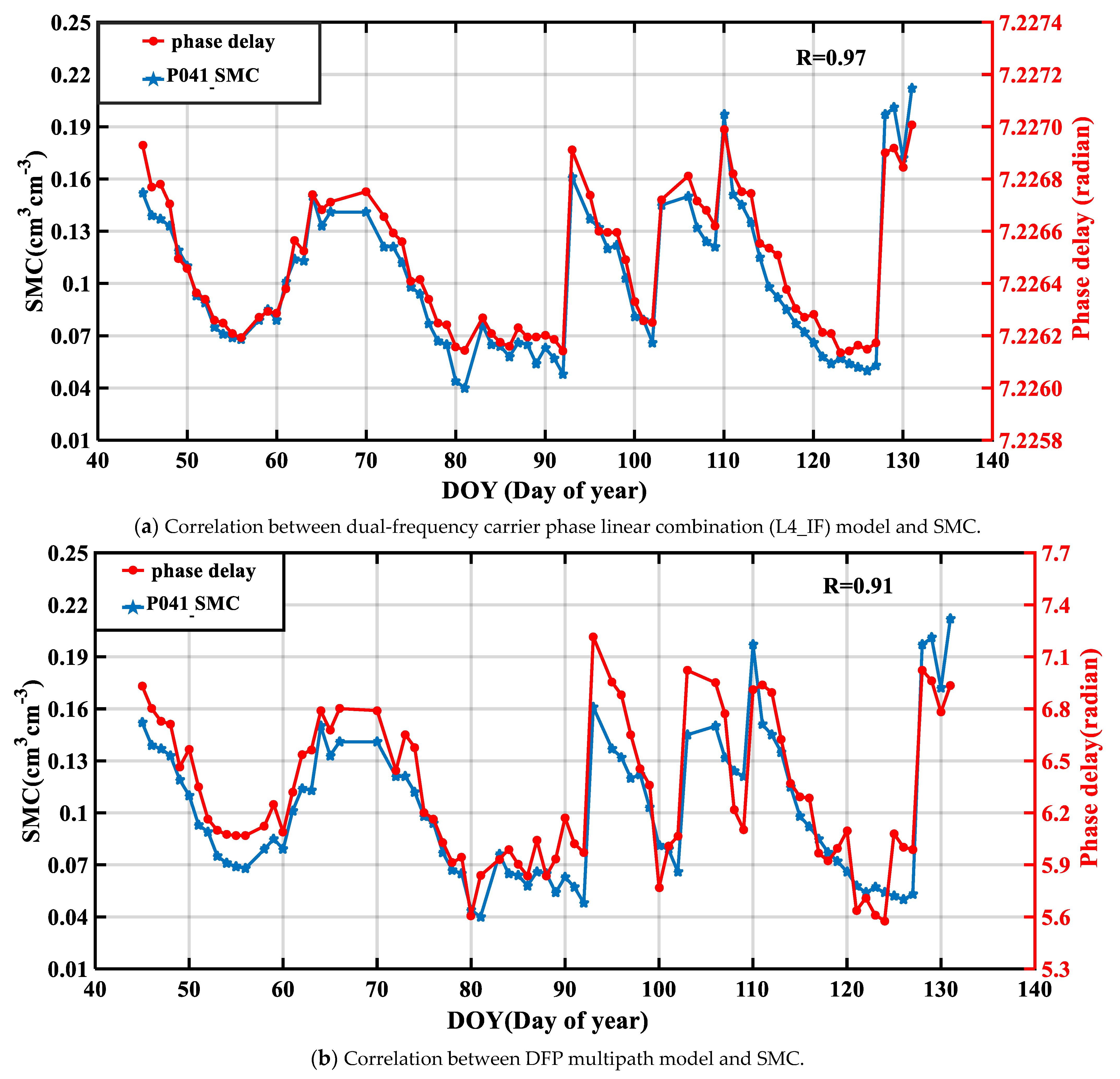
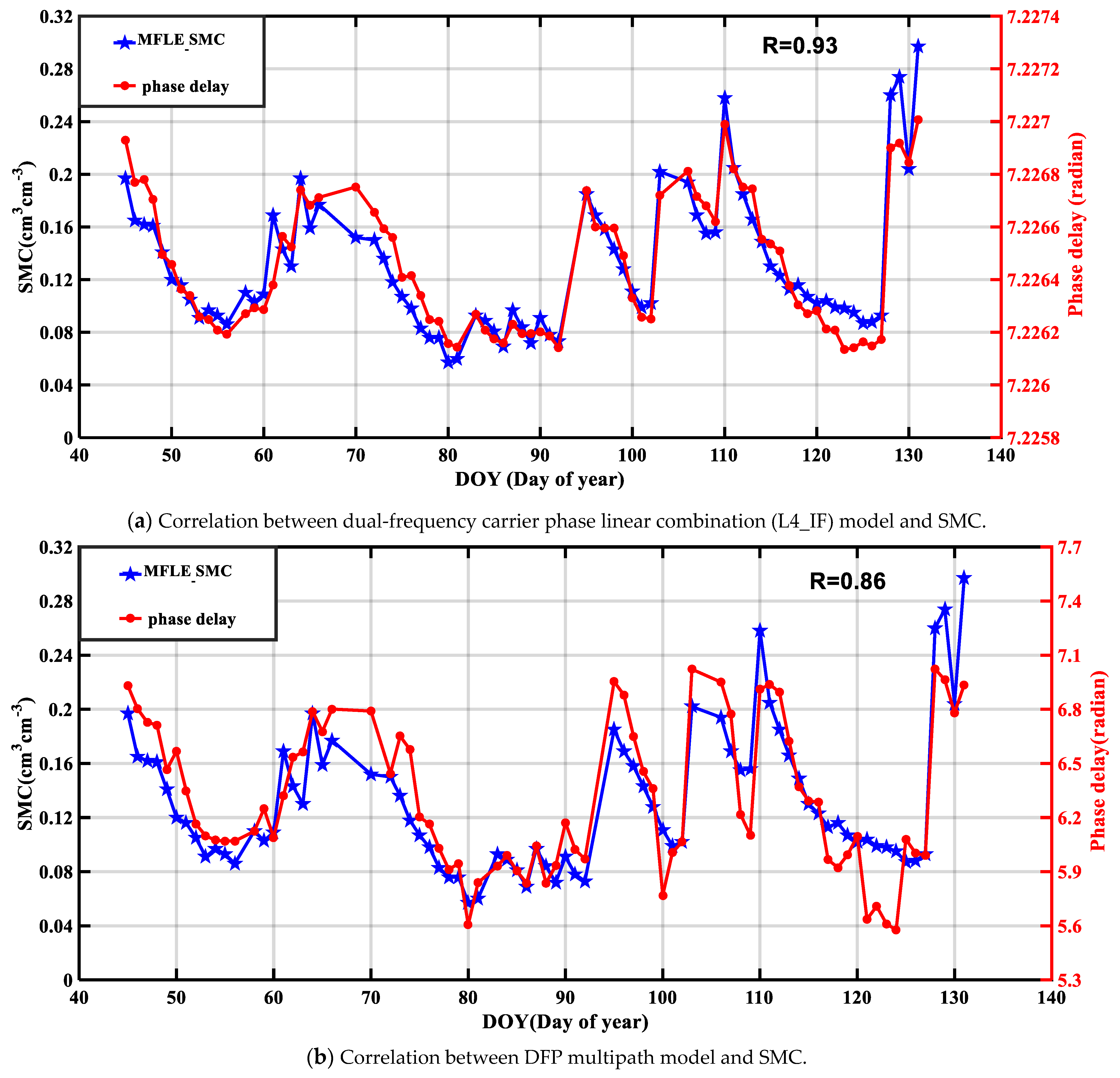
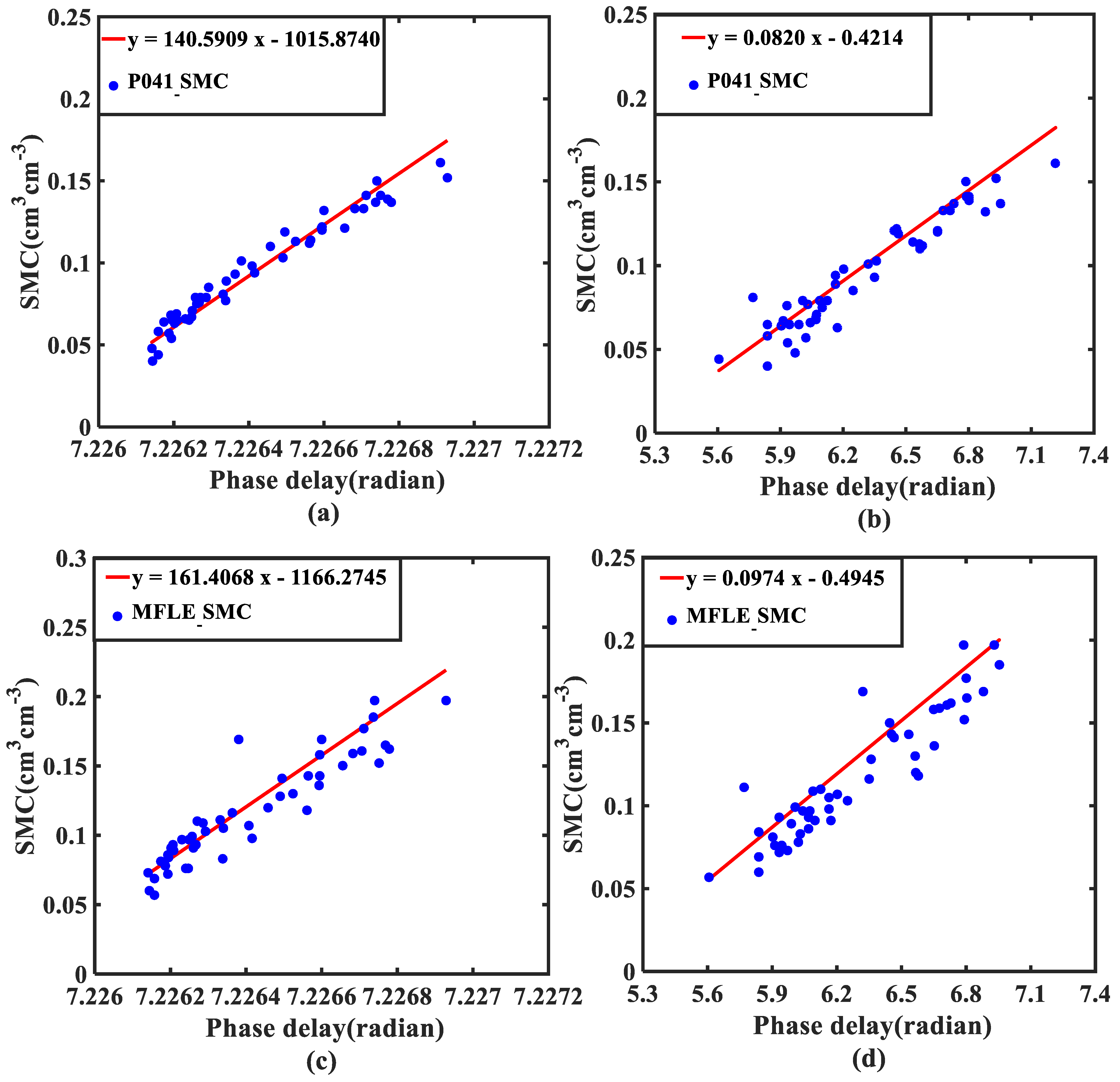
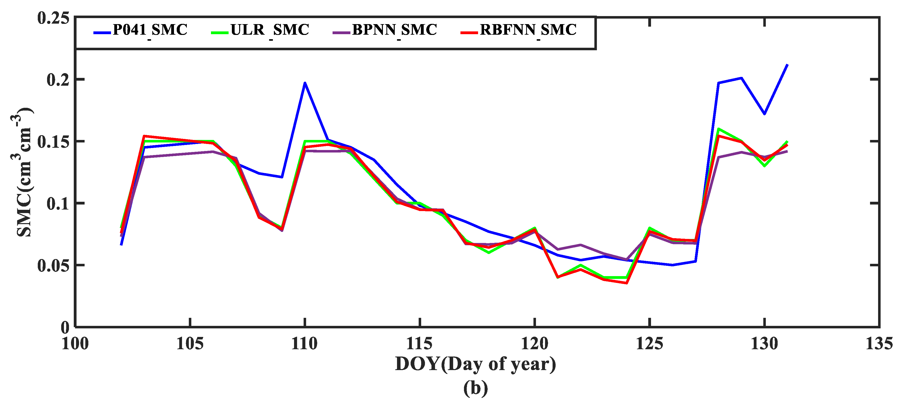
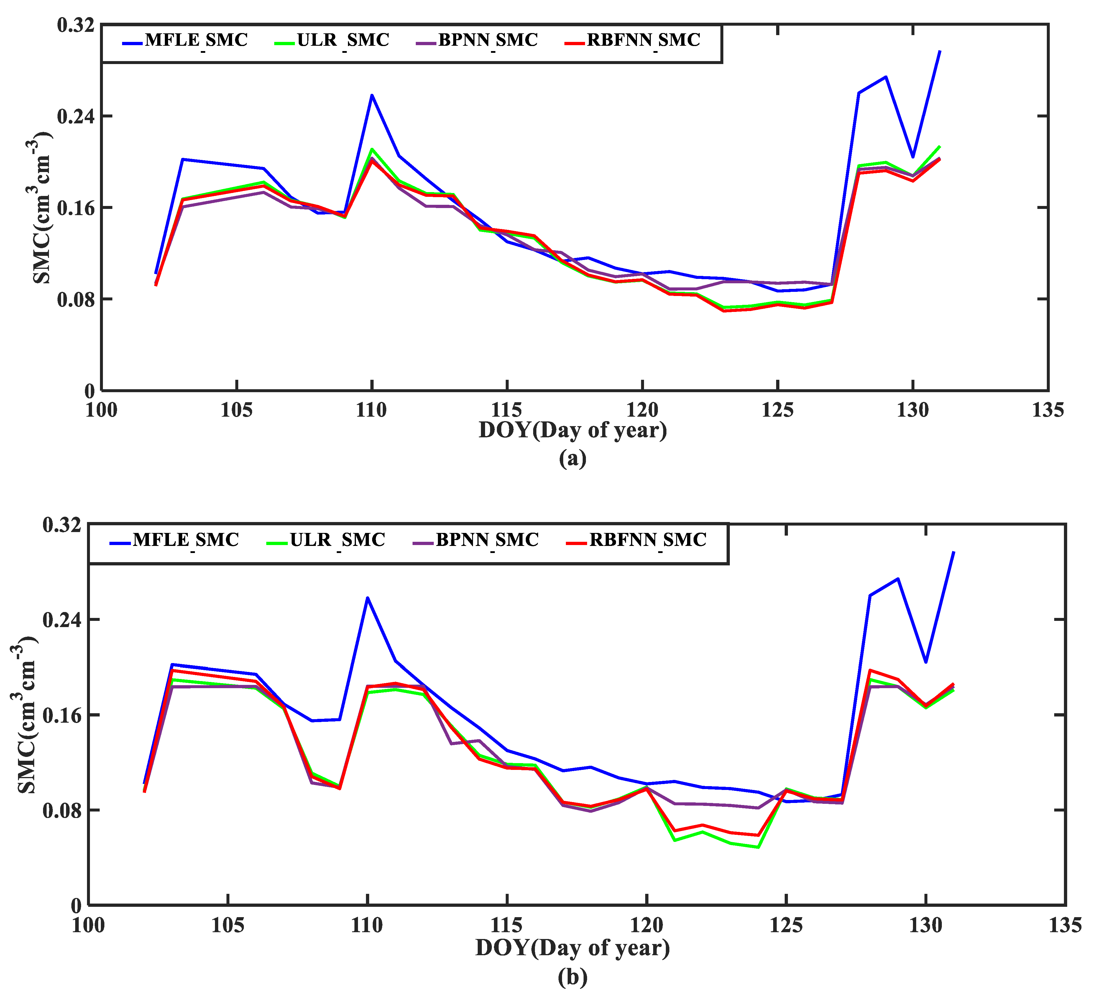
The delay phases obtained by the multipath error solution and the soil moisture are strongly correlated. For the P041 station, the R values of the L4_IF and DFP methods are 0.97 and 0.91, respectively. For the MFLE station, the R values of the L4_IF and DFP methods are 0.93 and 0.86, respectively. Because the observation error of the L4 linear combination is low and the change in the ionospheric delay in the short term is small, we used the high-order fitting to further weaken the influence of the ionospheric delay. The L4_IF method has higher R and soil moisture estimation accuracy than the DFP method. When the BPNN model, RBFNN model and ULR model are used to predict soil moisture, the results show that the prediction results of the BPNN model are better than the RBFNN model and ULR model, and the RBFNN model is slightly better than the ULR model. The results show that BPNN can improve the inversion accuracy of GNSS-IR soil moisture.
(2)
Since the calculation of the phase delay only requires a small amount of multipath error compared to the soil moisture retrieval based on the SNR, the proposed method does not require the diagnostic signal frequency, and only a tiny number of epoch multipath errors needs to be used to calculate the delay phase. So, achieving high-time-resolution GNSS-IR SMC retrieval is easier. Therefore, this method can be used to easily obtain high-time-resolution and accurate soil moisture estimations.
(3)
Given the changes in soil moisture, the reflectivity of the surface changes, which in turn will lead to changes in the amplification, attenuation factor κ , and phase delay. A further new finding is that the phase delay and the amplification attenuation factor κ based on the L4_IF method show the same change trend, and the Pearson correlation coefficient between them is 1. Conversely, the phase delay based on the MP2 method and the amplification attenuation factor κ show the opposite trend, and the Pearson correlation coefficient between them is −1. These results show that the phase delay is closely related to the amplification attenuation factor κ . In other words, the amplification and attenuation factor κ can also be used for soil moisture estimation, which can obtain the same result as the phase delay. For the sake of brevity, this article does not list the research results of the amplification and attenuation factor κ .
If SNR does not exist in the original file of GNSS and the number of GNSS satellites with triple-frequency signals is still limited, the L4_IF method and DFP method proposed in this paper can be used as alternative methods for monitoring through GNSS-IR so as to enrich the data source of GNSS-IR soil moisture inversion and improve the ability of GNSS to serve environmental monitoring. However, it should be noted that not all satellite observations are suitable for estimating soil moisture, and different satellite selections will lead to different results. Therefore, the effective selection of satellites is still a challenge. Because this method does not need to diagnose the signal frequency and only needs less epoch multipath error to calculate the delay phase, it is easier to achieve higher time resolution of GNSS-IR soil moisture inversion. Soil moisture inversion based on a multipath error enriches GNSS-IR data sources and enhances the reliability of GNSS-IR.

Author Contributions

Conceptualization, Y.W., J.T. and P.L.; methodology, S.N.; formal analysis, J.X., N.L., M.W. and P.L.; data curation, J.X., D.H. and J.S.; writing—original draft preparation, S.N.; writing—review and editing, Y.W. and J.T.; supervision, Y.W. and J.T. All authors have read and agreed to the published version of the manuscript.

Funding

This research was funded by the Anhui Educational Commission Key Project, grant numbers: KJ2020A00706, KJ2021A1077, KJ2021A1078, KJ2021A1084; the Chuzhou Science and Technology Guidance Program Project, grant number: 2021ZD009; the Anhui Educational Commission General Project, grant number: KJ2021B08, KJ2021B07.

Data Availability Statement

The GNSS site data were provided under the PBO Observation Program of the United States, and the measured soil moisture data were obtained from https://cires1.colorado.edu/portal (accessed on 10 September 2021) and https://data.unavco.org/archive/gnss/products (accessed on 10 September 2021).

Acknowledgments

We thank the PBO Observation Program of the United States for providing the GNSS data, and the University of Colorado for providing data for soil moisture comparison analysis.

Conflicts of Interest

The authors declare no conflict of interest.

References

  1. Seneviratne, S.I.; Corti, T.; Davin, E.L.; Hirschi, M.; Jaeger, E.B.; Lehner, I.; Orlowsky, B.; Teuling, A.J. Investigating soil moisture–climate interactions in a changing climate: A review. Earth-Sci. Rev. 2010, 99, 125–161. [Google Scholar] [CrossRef]
  2. Ray, R.L.; Jacobs, J.M. Relationships among remotely sensed soil moisture, precipitation and landslide events. Nat. Hazards. 2007, 43, 211–222. [Google Scholar] [CrossRef]
  3. Wanders, N.; Karssenberg, D.; de Roo, A.; de Jong, S.M.; Bierkens, M.F.P. The suitability of remotely sensed soil moisture for improving operational flood forecasting. Hydrol. Earth Syst. Sci. 2014, 18, 2343–2357. [Google Scholar] [CrossRef] [Green Version]
  4. Schaufler, G.; Kitzler, B.; Schindlbacher, A.; Skiba, U.; Sutton, M.A.; Zechmeister-Boltenstern, S. Greenhouse gas emissions from European soils under different land use: Effects of soil moisture and temperature. Eur. J. Soil Sci. 2010, 61, 683–696. [Google Scholar] [CrossRef]
  5. Jin, S.; Zhang, Q.; Zhang, X. New Progress and Application Prospects of Global Navigation Satellite System Reflectometry (GNSS + R). Acta Geod. Cartogr. Sin. 2017, 46, 1389–1398. [Google Scholar] [CrossRef]
  6. Wan, W.; Chen, X.; Peng, X.; Huang, B.; Ming, X.; Hong, L.; Min, Z.; Pang, X.; Ting, Y.; Chang, Y.; et al. Overview and outlook of GNSS remote sensing technology and applications. J. Remote Sens. 2016, 20, 858–874. (In Chinese) [Google Scholar] [CrossRef]
  7. Ge, L.; Han, S.; Rizos, C. Multipath Mitigation of Continuous GPS Measurements Using an Adaptive Filter. GPS Solut. 2000, 4, 19–30. [Google Scholar] [CrossRef]
  8. Li, Y.; Chang, X.; Yu, K.; Wang, S.; Li, J. Estimation of snow depth using pseudorange and carrier phase observations of GNSS single-frequency signal. GPS Solut. 2019, 23, 118. [Google Scholar] [CrossRef]
  9. Ozeki, M.; Heki, K. GPS snow depth meter with geometry-free linear combinations of carrier phases. J. Geod. 2012, 86, 209–219. [Google Scholar] [CrossRef] [Green Version]
  10. Larson, K.M.; Small, E.E.; Gutmann, E.; Bilich, A.; Axelrad, P.; Braun, J. Using GPS multipath to measure soil moisture fluctuations: Initial results. GPS Solut. 2008, 12, 173–177. [Google Scholar] [CrossRef]
  11. Larson, K.M.; Small, E.E.; Gutmann, E.; Bilich, A. Use of GPS receivers as a soil moisture network for water cycle studies. Geophys. Res. Lett. 2008, 35, 851–854. [Google Scholar] [CrossRef] [Green Version]
  12. Larson, K.M.; Braun, J.J.; Small, E.E.; Zavorotny, V.; Gutmann, E.; Bilich, A. GPS multipath and its relation to near-surface soil moisture content. IEEE J. Sel. Top. Appl. Earth Obs. Remote Sens. 2010, 3, 91–99. [Google Scholar] [CrossRef]
  13. Zhang, S.; Wang, T.; Wang, L.; Zhang, J.; Peng, J.; Liu, Q. Evaluation of GNSS-IR for Retrieving Soil Moisture and Vegetation Growth Characteristics in Wheat Farmland. J. Surv. Eng. 2021, 147, 04021009. [Google Scholar] [CrossRef]
  14. Liang, Y.; Ren, C.; Wang, H.; Huang, Y.; Zheng, Z. Research on soil moisture inversion method based on GA-BP neural network model. Int. J. Remote Sens. 2019, 40, 2087–2103. [Google Scholar] [CrossRef]
  15. Han, M.; Zhu, Y.; Yang, D.; Hong, X.; Song, S. A Semi-Empirical SNR Model for Soil Moisture Retrieval Using GNSS SNR Data. Remote Sens. 2018, 10, 280. [Google Scholar] [CrossRef] [Green Version]
  16. Jin, L.; Yang, L.; Han, M.; Hong, X.; Sun, B.; Liang, Y. Soil moisture inversion method based on GNSS-IR dual frequency data fusion. J. Beijing Univ. Aeronaut. Astronaut. 2019, 45, 1248. [Google Scholar] [CrossRef]
  17. Ran, Q.; Zhang, B.; Yao, Y.; Li, J. Editing arcs to improve the capacity of GNSS-IR for soil moisture retrieval in undulating terrains. GPS Solut. 2022, 26, 1–11. [Google Scholar] [CrossRef]
  18. Han, M.; Zhu, Y.; Yang, D.; Chang, Q.; Hong, X.; Song, S. Soil moisture monitoring using GNSS interference signal: Proposing a signal reconstruction method. Remote Sens. Lett. 2020, 11, 373–382. [Google Scholar] [CrossRef]
  19. Li, Y.; Yu, K.; Jin, T.; Chang, X.; Zhang, Q.; Xu, C.; Li, J. Soil moisture estimation using amplitude attenuation factor of low-cost GNSS receiver based SNR observations. In Proceedings of the 2021 IEEE International Geoscience and Remote Sensing Symposium IGARSS, Brussels, Belgium, 11–16 July 2021; pp. 7654–7657. [Google Scholar] [CrossRef]
  20. Roussel, N.; Frappart, F.; Ramillien, G.; Darrozes, J.; Baup, F.; Lestarquit, L.; Ha, M.C. Detection of soil moisture variations using GPS and GLONASS SNR data for elevation angles ranging from 2° to 70°. IEEE J. Sel. Top. Appl. Earth Obs. Remote Sens. 2016, 9, 4781–4794. [Google Scholar] [CrossRef]
  21. Yu, K.; Ban, W.; Zhang, X.; Yu, X. Snow Depth Estimation Based on Multipath Phase Combination of GPS Triple-Frequency Signals. IEEE Trans. Geosci. Remote Sens. 2015, 53, 5100–5109. [Google Scholar] [CrossRef]
  22. Zhang, X.; Nie, S.; Zhang, C.; Zhang, J.; Cai, H. Soil moisture estimation based on triple-frequency multipath error. Int. J. Remote Sens. 2021, 42, 5953–5968. [Google Scholar] [CrossRef]
  23. Shen, F.; Sui, M.; Zhu, Y.; Cao, X.; Ge, Y.; Wei, H. Using BDS MEO and IGSO Satellite SNR Observations to Measure Soil Moisture Fluctuations Based on the Satellite Repeat Period. Remote Sens. 2021, 13, 3967. [Google Scholar] [CrossRef]
  24. Bilich, A.; Larson, K.M. Mapping the GPS multipath environment using the signal-to-noise ratio (SNR). Radio Sci. 2007, 42, 1–16. [Google Scholar] [CrossRef]
  25. Zhang, Z.; Guo, F.; Zhang, X. Triple-frequency multi-GNSS reflectometry snow depth retrieval by using clustering and normalization algorithm to compensate terrain variation. GPS Solut. 2020, 24, 52. [Google Scholar] [CrossRef]
  26. Lv, J.; Zhang, R.; Yu, B.; Pang, J.; Liao, M.; Liu, G. A GPS-IR Method for Retrieving NDVI from Integrated Dual-Frequency Observations. IEEE Geosci. Remote Sens. Lett. 2021, 19, 1–5. [Google Scholar] [CrossRef]
  27. Wang, N.; Xue, T.; Gao, F.; Xu, G. Sea Level Estimation Based on GNSS Dual-Frequency Carrier Phase Linear Combinations and SNR. Remote Sens. 2018, 10, 470. [Google Scholar] [CrossRef] [Green Version]
  28. Katzberg, S.J.; Torres, O.; Grant, M.S.; Masters, D. Utilizing calibrated GPS reflected signals to estimate soil reflectivity and dielectric constant: Results from SMEX02. Remote Sens. Environ. 2006, 100, 17–28. [Google Scholar] [CrossRef] [Green Version]
  29. Yu, K.; Li, Y.; Chang, X. Snow Depth Estimation Based on Combination of Pseudorange and Carrier Phase of GNSS Dual-Frequency Signals. IEEE Trans. Geosci. Remote Sens 2019, 57, 1817–1828. [Google Scholar] [CrossRef]
  30. Chew, C.; Small, E.E.; Larson, K.M. An algorithm for soil moisture estimation using GPS-interferometric reflectometry for bare and vegetated soil. GPS Solut. 2015, 20, 525–537. [Google Scholar] [CrossRef]
Figure 1. Schematic diagram of GNSS-IR SMC retrieval. After the satellite sends the signal, the right-handed circular polarized (RHCP) antenna receives the direct signal and the surface reflected signal, producing an interference effect at the receiver. A is the GNSS receiver antenna; B is the reflection point position of GNSS satellite signals passing through the ground; O is the footing point of the vertical line between the over-reflection point and the GNSS satellite direct signal; θ is the elevation angle of the satellite; S 1 is the direct satellite signal received by the receiver antenna; S 2 is the reflected signal reflected by the object’s surface around the receiver antenna and enters the antenna; H is the vertical height from the antenna phase center to the ground.
Remotesensing 14 03193 g001
Figure 2. GNSS test site locations. P041 and MFLE stations, Boulder, CO, USA.
Remotesensing 14 03193 g002
Figure 3. Station conditions: (a) Environment around P041 station; (b) environment around MFLE station. Note: GNSS test site locations: P041 and MFLE, Boulder, CO, USA (https://www.unavco.org) (accessed on 25 September 2021).
Remotesensing 14 03193 g003
Figure 4. The soil moisture rainfall diagram during the experimental period.
Remotesensing 14 03193 g004
Figure 5. The technical process we followed for multisatellite dual-frequency combined multipath error SMC retrieval. Note: RTKLIB is an open-source program package for standard and precise positioning with GNSS (global navigation satellite system). RTKLIB consists of a portable program library and several APs (application programs) utilizing the library (http://www.rtklib.com/) (accessed on 10 February 2022).
Remotesensing 14 03193 g005
Figure 6. Changes in the elevation angles of almost all GPS satellites at P041.
Remotesensing 14 03193 g006
Figure 7. The multipath error varies with satellite elevation angle: (a) dual-frequency pseudorange multipath error; (b) dual-frequency carrier phase linear combination of multipath errors.
Remotesensing 14 03193 g007
Figure 8. The multipath error of low elevation angle varies with the sine value of satellite elevation angle: (a) the dual-frequency pseudo multipath error MP2; (b) the dual-frequency carrier phase linear combination multipath error L4_IF for removing ionospheric delay.
Remotesensing 14 03193 g008
Figure 9. The projected trajectory of the P041 (DOY: 2014-065) satellite at an elevation of 5–25°.
Remotesensing 14 03193 g009
Figure 10. First Fresnel reflection region for GPS L2 frequency at different elevation angles.
Remotesensing 14 03193 g010
Figure 11. First Fresnel reflection region map of station P041 (DOY: 2014-065): GPS satellite distribution in the first Fresnel reflection region of station P041 when satellite elevation angle was (a) 10°; (b) 25°.
Remotesensing 14 03193 g011
Figure 12. Multisatellite dual-frequency combined multipath error Lomb–Scargle periodogram. Spectrum analysis diagrams of the (a,c) dual-frequency carrier phase combined multipath error (L4_IF;) (b,d) dual-frequency pseudorange multipath error (MP2).
Remotesensing 14 03193 g012
Figure 13. P041 station; correlation between Delay Phase and SMC.
Remotesensing 14 03193 g013
Figure 14. MFLE station; correlation between Delay Phase and SMC.
Remotesensing 14 03193 g014
Figure 15. For the P041 station; scatter diagram of the SMC and regression equation based on (a) the L4_IF method; (b) the DFP multipath model. For the MFLE station; scatter diagram of the SMC and regression equation based on (c) the L4_IF method; (d) the DFP multipath model.
Remotesensing 14 03193 g015
Figure 16. For P041 station; comparison between the predicted values of three models and measured values of soil moisture (a) the L4_IF method; (b) the DFP multipath model.
Remotesensing 14 03193 g016aRemotesensing 14 03193 g016b
Figure 17. For the MFLE station, comparison between predicted values of three models and measured values of soil moisture (a) the L4_IF method; (b) the DFP multipath model. Note: The P041_SMC in Figure 16a,b are SMC value of the P041 station; the MFLE_SMC in Figure 17a,b are SMC values of the MFLE station; the ULR_SMC in Figure 16 and Figure 17 are unitary linearity regression model predictive value; the BPNN_SMC in Figure 16 and Figure 17 are back propagation neural network model predictive value; the RBFNN_SMC in Figure 16 and Figure 17 are radial basis function neural network model predictive value.
Remotesensing 14 03193 g017
Table 1. Receiver and its related parameters at the P041 site.
ProjectParameter
Type of receiverPOLARX5
Sampling interval15 s
Type of antennaTRM59800.80
Antenna height1.90 m
Table 2. Satellite selection results at site P041 on 6 March 2014 (DOY: 2014-065).
Observation Period NumberGPS Satellite Number (PRN)Azimuth
(/°)
Height Angle
(/°)
GPS Time
(hh:mm:ss)
1PRN16170.75–171.166.08–7.0501:28:45–01:31:15
2PRN0344.55–44.6814.72–15.6903:28:45–03:31:15
3PRN26239.89–240.8224.45–25.2505:58:45–06:01:15
4PRN2050.47–51.4612.70–12.9407:58:45–08:01:15
5PRN24221.92–222.6513.37–14.2209:58:45–10:01:15
6PRN0467.64–68.267.66–8.4611:28:45–11:31:15
7PRN15156.52–157.0914.87–15.8212:28:45–12:31:15
8PRN0557.21–57.6911.33–12.2114:28:45–14:31:15
9PRN16275.01–275.946.19–6.7315:28:45–15:31:15
10PRN31184.73–184.918.41–9.4717:58:45–18:01:15
11PRN2573.92–75.1122.27–22.4719:58:45–20:01:15
12PRN16170.75–171.176.09–7.0520:58:45–21:01:15
Table 3. Statistical table for accuracy comparison between L4_IF and DFP methods.
Station IDMethodCorrelation Coefficient (R)STD (cm3 cm−3)MAE (cm3 cm−3)RMSE (cm3 cm−3)
P041L4_IF0.970.0400.0370.014
DFP0.910.0400.0380.026
MFLEL4_IF0.930.0470.0430.029
DFP0.860.0470.0490.042
Note: The STD in Table 3 is the error standard deviation; the MAE in Table 3 is mean absolute error; the RMSE in Table 3 is root-mean squared error.
Table 4. Statistical table for precision comparison of three models of L4_IF and DFP methods.
Station IDMethodModelSTD (cm3 cm−3)MAE (cm3 cm−3)
P041L4_IFULR0.0400.037
BPNN0.0390.034
RBFNN0.0390.035
DFPULR0.0400.038
BPNN0.0330.033
RBFNN0.0390.038
MFLEL4_IFULR0.0470.043
BPNN0.0390.037
RBFNN0.0450.042
DFPULR0.0470.049
BPNN0.0420.046
RBFNN0.0470.049
Note: The STD in Table 4 is error standard deviation; the MAE in Table 4 is mean absolute error; the ULR in Table 4 is unitary linearity regression; the BPNN in Table 4 is back propagation neural network; the RBFNN in Table 4 is radial basis function neural network.
Publisher’s Note: MDPI stays neutral with regard to jurisdictional claims in published maps and institutional affiliations.

